Groupoidification Made Easy

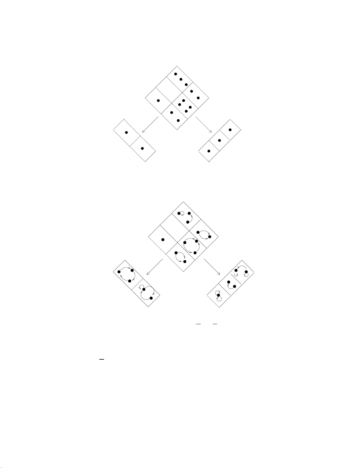
Group oidiﬁcation Made Easy John C. Baez, Alexander E. Hoﬀnung, and Christopher D. W alk er Departmen t of Mathematics, Unive rsit y of Califo rnia Riv erside, CA 92521 USA Ma y 29, 2018 Abstract Group o idiﬁcation is a form of categoriﬁcation in whic h ve ctor spaces are replaced by group oids, and linear op erators are rep la ced b y spans of group oi ds. W e introdu ce this i dea with a detailed exp osition of ‘de- group oidiﬁcation’: a systematic process that turns group oids and span s into vector spaces and linear op era tors. Then w e present t wo applications of group oidiﬁcation. The ﬁrst is to F eynman diagrams. The Hilb ert space for the quantum harmonic oscillator arises naturally from degroup oidif y- ing th e group oi d of ﬁnite sets and bijections. This allo ws for a p urely com binatorial interpretation of creation and annihilation operators, their comm utation relations, ﬁeld op erato rs, their normal-ordered p o w ers, and ﬁnally F eyn man diagrams. The second application is to Hec ke algebras. W e explain h o w to group oidify the Heck e algebra associated to a Dynkin diagram whenever the deformation parameter q is a prime p o w er. W e illustrate this with the simplest n o ntrivial example, coming from the A 2 Dynkin diagram. In this ex ample we sho w t h at the solutio n of the Y ang– Baxter equation built into the A 2 Heck e algebra arises naturally from the axioms of pro jective geometry applied to the pro jective p la ne ov er the ﬁnite ﬁeld F q . 1 In tro duction ‘Group oidiﬁcation’ is an attempt to exp ose the combinatorial underpinnings of linear a lgebra — the har d b ones of set theory underlying the ﬂexibility o f the contin uum. One of the main less ons of mo dern algebra is to av oid choosing bases for vector s paces until you need them. As Hermann W eyl wro te, “The int ro duction of a coo rdinate system to geometry is an act of violence”. But vec- tor spaces often come equipp ed with a natura l basis — and when this happ ens, there is no harm in ta k ing adv an tage of it. The most obvious example is when our vector space has b een deﬁned to cons ist of formal linear combinations of the elements of s ome set. Then this set is our basis. But sur prisingly often, the elements o f this set a re isomorphism classes of obje cts in some gr oup oid . This is w he n gro upoidiﬁcation can b e useful. It lets us work directly with the 1 group oid, using to ols analogous to tho se of linear alg ebra, without bringing in the r eal num b e r s (or any other ground ﬁeld). F or example, let E b e the group oid of ﬁnite sets and bijections. A n iso mor- phism c la ss of ﬁnite se ts is just a natura l n umber, so the set o f isomorphism classes of ob jects in E can b e ident iﬁed with N . Indeed, this is why natural nu mbers were inv en ted in the ﬁrst place: to count ﬁnite sets. The r eal vector space with N as basis is usually identiﬁed with the p olynomial algebra R [ z ], since that has bas is z 0 , z 1 , z 2 , . . . . Alternatively , w e can work with inﬁnite for- mal linear co m binations of natura l num ber s, whic h form the alg ebra of formal power series, R [[ z ]]. So, formal p o wer series should b e imp ortant when we apply the to ols of linear alg ebra to study the gro up oid of ﬁnite sets. Indeed, formal p o wer series hav e long b een used as ‘genera ting functions’ in combinatorics [21]. Given a com binator ia l structur e we can put on ﬁnite s ets, its generating function is the formal pow er s eries whose n th coeﬃcient s ays how many wa ys we can put this s tructure on an n - e lemen t set. Andr ´ e Joyal formalized the idea of ‘a structure we c an put on ﬁnite sets’ in terms o f esp` ec es de structur es , or ‘structure t yp es’ [6, 14, 15]. La ter his work w as gener alized to ‘stuﬀ types’ [4], which a re a key ex ample of gr oupoidiﬁcation. Heuristically , a s tuﬀ type is a way of equipping ﬁnite sets with a sp eciﬁc t yp e of extr a s tuﬀ — for ex ample a 2-colo ring, or a linear or dering, or an additional ﬁnite set. Stuﬀ types have g enerating functions, whic h are for mal power serie s . Combinatorially in teresting o perations on stuﬀ types co r respond to in teresting o perations on their gener a ting functions: addition, multiplication, diﬀerentiation, and so on. Joy al’s great idea a moun ts to this: work dir e ctly with stuﬀ t yp es as much as p ossible, and put oﬀ t a king their gener ating functions. As we shall see, this is an example of group oidiﬁcation. T o see how th is works, we should be more precise. A stuﬀ t yp e is a g roupoid ov er the g roupoid of ﬁnite sets: that is, a group oid Ψ eq uipped with a functor v : Ψ → E . The r eason for the funn y name is that we can think of Ψ as a group oid of ﬁnite sets ‘equipp ed with extra stuﬀ ’. The functor v is then the ‘forgetful functor’ that forgets this extra stuﬀ and gives the underlying set. The gener ating function of a stuﬀ type v : Ψ → E is the formal p o wer series Ψ e ( z ) = ∞ X n =0 | v − 1 ( n ) | z n . (1) Here v − 1 ( n ) is the ‘ess en tial inv erse imag e’ of any n -element set, say n ∈ E . W e deﬁne this term later, but the idea is straig h tforward: v − 1 ( n ) is the group oid of n -element sets equipp ed with the given type of stuﬀ. The n th co eﬃcien t of the g enerating function measur es the size of this g roupoid. But how? Here we need the concept of gr oup oi d c ar dina lity . It seems this concept ﬁrst appea r ed in algebraic geometry [5, 16]. W e rediscov ered it by po ndering the meaning of division [4]. Addition of natura l n um b ers comes from disjoint union of ﬁnite sets, since | S + T | = | S | + | T | . 2 Multiplication comes from cartesian pro duct: | S × T | = | S | × | T | . But wha t ab out div is ion? If a gro up G acts o n a set S , w e can ‘divide’ the set by the g roup and form the quo tien t S/G . If S and G are ﬁnite and G a cts fre e ly on S , S/G r eally deserves the name ‘quotien t’, since then | S/G | = | S | / | G | . Indeed, this fact ca ptur es some of our naive in tuitions ab out division. F or example, why is 6 / 2 = 3? W e can take a 6- elemen t set S with a free action of the g roup G = Z / 2 and cons truct the set o f orbits S/G : Since we are ‘fo lding the 6-element set in half ’, we get | S/G | = 3. The trouble starts when the a ction of G on S fails to b e free. Let’s try the same trick star ting with a 5 -elemen t set: W e don’t obtain a set with 2 1 2 elements! The reas o n is that the p oin t in the middle gets mapped to itself. T o get the desir ed ca rdinalit y 2 1 2 , we would need a wa y to count this p oin t a s ‘fo lde d in half ’. T o do this, we should ﬁrst repla ce the ordina ry quotient S/G b y the ‘actio n group oid’ or ‘weak quotient’ S/ /G . This is the group oid where ob jects are elements of S , a nd a morphism from s ∈ S to s ′ ∈ S is an element g ∈ G with g s = s ′ . Comp osition of morphisms works in the ob vious way . Nex t, we should deﬁne the ‘cardinality’ of a group oid as follows. F or each isomorphism class of ob jects, pick a repr esen tative x and compute the recipro cal of the num ber of automorphisms of this ob ject; then sum the r esult ov er isomorphism classes. In other words, deﬁne the cardinality of a group oid X to b e | X | = X isomorphism c lasses of ob jects [x] 1 | Aut( x ) | . (2) 3 With these deﬁnitions, o ur problema tic example g iv es a gro upoid S/ /G w ith cardinality 2 1 2 , since the p oin t in the middle o f the picture gets counted as ‘half a p oin t’. In fact, | S/ / G | = | S | / | G | whenever G is a ﬁnite group acting on a ﬁnite set S . The concept o f group oid car dina lit y gives an eleg an t deﬁnition of the g e ner- ating function of a stuﬀ type — Eq. 1 — which matches the us ual ‘expo nen tial generating function’ from combinatorics. F or the details of how this works, see Example 1 1. Even b etter, we can v astly generalize the notion of gener a ting function, b y replacing E with a n arbitrar y group oid. F or any group oid X w e get a vector space: namely R X , the space o f functions ψ : X → R , wher e X is the set o f isomorphism classes of o b jects in X . A ny suﬃciently nice group oid over X gives a vector in this v ector space. The question then arises: what ab out linear op erators ? Her e it is g oo d to take a less o n from Heisenber g ’s matrix mechanics. In his early work on q uan tum mechanics, Heisen b erg did not know ab out matrices. He reinv ented them based on this idea: a matrix S can describ e a quant um pro cess by letting the matrix ent ry S j i ∈ C stand for the ‘amplitude’ for a system to undergo a tra nsition from its i th state to its j th state. The meaning of complex amplitudes was somewhat mysterious — and indeed it remains so, muc h as we ha ve b ecome accustomed to it. Howev er, the mystery ev apora tes if we hav e a matrix whose e n tries are natura l num ber s. The n the matrix entry S j i ∈ N simply counts the numb er of ways for the sys tem to undergo a transition fro m its i th state to its j th state. Indeed, let X b e a set whose elements are pos sible ‘initial states’ fo r some system, and let Y be a set who se elements ar e poss ible ‘ﬁnal states’. Suppo se S is a set equipp ed with maps to X and Y : S q          p   @ @ @ @ @ @ @ Y X Mathematically , we call this setup a span of sets. Physically , w e ca n think o f S as a set of p ossible ‘even ts’. Point s in S sitting ov er i ∈ X and j ∈ Y form a subset S j i = { s : q ( s ) = j, p ( s ) = i } . W e can think of this a s the set of ways for the system to under go a transition from its i th state to its j th state. Indee d, we can picture S mor e vividly as a matrix o f sets: 4 q p X Y S If all the sets S j i are ﬁnite, we get a matrix o f natural num ber s | S j i | . Of course , matrices of natural num b ers only allow us to do a limited p ortion of linear algebr a. W e can go further if we co nsider, no t spans of sets, but sp ans of gr oup oids . W e ca n picture one of these roughly as follo ws: q p X Y S If a span o f group oids is suﬃcie ntly nice — o ur tec hnical ter m will be ‘tame’ — we can conv ert it in to a linear o perator from R X to R Y . Viewed as a matrix, this op erator will hav e nonnegative real matrix en tries. So , w e hav e not s uc c eeded in ‘gro upoidifying’ full-ﬂedged qua n tum mec hanics, wher e the matrices can b e complex. Still, w e have made some pr ogress. As a sign of this, it turns o ut that any gro upoid X giv es not just a vector space R X , but a real Hilbe rt space L 2 ( X ). If X = E , the complexiﬁcatio n of this Hilber t spa ce is the Hilb ert space of the quantum harmonic oscillato r. The quantum harmonic o scillator is the simplest system where we can see the usual to ols of quan tum ﬁe ld theory at work: for example, F eynman diagrams. It turns out that larg e p ortions of the theory o f F eynman dia grams can b e done with spans of group oids replacing op erators [4 ]. The combinatorics of thes e dia g rams 5 then beco mes vivid, str ipp ed bare of the trappings of ana lysis. W e sketc h how this works in Section 3.1. A more detailed trea tmen t can be found in the work of Jeﬀrey Morton [1 9 ]. T o ge t complex num b ers into the game, Mor to n gener alizes group oids to ‘group oids over U(1)’: that is, group oids X equippe d with functors v : X → U(1), wher e U(1) is the group oid with unit co mplex num ber s as ob jects and only ident ity morphisms. The cardinality of a g roupoid ov er U(1) ca n be complex. Other genera liz ations of group oid ca rdinalit y are a lso in teresting. F or ex a m- ple, Leinster has gener alized it to categor ies [17]. The cardinality o f a catego ry can be neg ativ e! Mo re recently , W einstein ha s generalize d it to Lie g roupoids [22]. Gettin g a useful genera liz ation o f group oids for which the cardinality is naturally co mplex, without putting in the complex n umbers ‘by hand’, remains an elusive goa l. How ev er, the work of Fior e a nd Leinster sug gests it is po ssible [9]. In the last few years James Dolan, T o dd T rimble and the author s hav e ap- plied g roupoidiﬁcatio n to structur es related to qua n tum gr oups, most notably Heck e alg ebras a nd Hall algebras . A b eautiful story has b egun to emerge in which q -deforma tion ar ises na turally fr om replacing the gr oupoid of ﬁnite sets by the gr oupoid o f ﬁnite-dimensional vector s paces ov er F q , wher e q is a prime power. T o some extent this work is a reinterpretation of known facts. How- ever, gr o upoidiﬁcation gives a conceptual framework for what befor e might have seemed a strange s et o f coincidences. W e hop e to wr ite up this material a nd develop it further in the y ears to come. F or now, the reader can turn to the online video s and notes av a ilable through U. C. Riverside [2]. The present pap er has a limited go a l: we wish to explain the basic ma chinery o f gr oupoidiﬁcation a s simply as po ssible. In Section 2, we present the basic facts about ‘degro upoidiﬁcation’: the pro cess that turns gro up oids into v ector spaces and tame spa ns into linear op- erators . Section 3 .1 descr ibes how to gr oupoidify the theo r y of F e ynman dia- grams; Sectio n 3.2 describ es ho w to g roupoidify the theory of Heck e alg ebras. In Section 4 we pr ove that the pro cess of degroup oidifying a tame span gives a well-deﬁned linear op erator. W e also giv e an explicit criterion for when a span of gr oupoids is tame, and explicit formula for the op erator coming from a tame span. Section 5 prov es man y o ther r esults stated earlier in the pa per. Ap- pendix A prov es some basic deﬁnitions and useful lemmas regarding gro upoids and spans of group oids. The goal is to make it eas y for reader s to try their own hand at group oidiﬁcation. 2 Degroup oidiﬁcation In this section w e describ e a systematic pro cess for turning group o ids in to vector spaces and tame spa ns in to linear op erators. This pro cess, ‘degroup oidiﬁcation’, is in fact a kind of functor. ‘Group oidiﬁcation’ is the attempt to undo this func- tor. T o ‘group oidify’ a piece of linear algebra means to take so me str uctur e built from vector space s and linear oper ators and try to ﬁnd interesting gro upoids and 6 spans that degroup oidify to g iv e this structure. So, to under s tand gr oupoidiﬁ- cation, we need to master degroup oidiﬁcation. W e b e g in b y des cribing how to turn a group oid into a vector spa c e. In what follows, all o ur group oids will be ‘essentially small’. This means that they hav e a set of isomor phis m cla sses o f ob jects, not a prop er class. W e also assume our group oids have ﬁnite homsets. In other words, giv en any pair of ob jects, the set of morphisms from one ob ject to another is ﬁnite. Deﬁnition 1. Given a gr oup oid X , let X b e the set of isomorphism classes of obje cts of X . Deﬁnition 2. Given a gr oup oid X , let the degroup oidiﬁcation of X b e the ve ctor sp ac e R X = { Ψ : X → R } . A nice example is the group oid o f ﬁnite sets and bijections: Example 3. Let E b e the gro upoid of ﬁnite sets a nd bijections. Then E ∼ = N , so R E ∼ = { ψ : N → R } ∼ = R [[ z ]] , where the formal pow er ser ie s asso ciated to a function ψ : N → R is given by: X n ∈ N ψ ( n ) z n . A suﬃciently nice group oid over a group oid X will give a vector in R X . T o construct this, we use the concept o f gr oupoid c ardinalit y: Deﬁnition 4. The cardinality of a gr oup oid X is | X | = X [ x ] ∈ X 1 | Aut( x ) | wher e | Aut( x ) | is the c ar dinality of the automorphism gr oup of an obje ct x in X . If t h is sum diver ges, we say | X | = ∞ . The cardinality of a gro upoid X is a well-deﬁned no nnegativ e ratio nal n um- ber whenever X and all the automorphism groups of o b jects in X a re ﬁnite. More gener ally , we s a y : Deﬁnition 5. A gr oup oid X is tame if | X | < ∞ . W e s ho w in Lemma 5 1 that given equiv alent group oids X and Y , | X | = | Y | . W e describe a useful a lternativ e metho d for computing group oid cardina lit y in Lemma 22. The r eason we us e R rather than Q as our gro und ﬁeld is that there ar e int eresting g roupoids who se cardinalities ar e irrationa l n umbers. The following example is fundamen tal: 7 Example 6. The g roupoid of ﬁnite s ets E has ca rdinalit y | E | = X n ∈ N 1 | S n | = X n ∈ N 1 n ! = e. With the co ncept of group oid cardinality in hand, we now descr ib e how to obtain a vector in R X from a suﬃciently nice g roupoid over X . Deﬁnition 7. Given a gr oup oid X , a group oid ov er X is a gr oup oid Ψ e quipp e d with a functor v : Ψ → X . Deﬁnition 8. Given a gr oup oid over X , say v : Ψ → X , and an obje ct x ∈ X , we deﬁne the ess en tial in v erse image of x , denote d v − 1 ( x ) , to b e the gr oup oid wher e: • an obje ct is an obje ct a ∈ Ψ such that v ( a ) ∼ = x ; • a morphism f : a → a ′ is any morphism in Ψ fr om a t o a ′ . Deﬁnition 9 . A gr oup oid over X , say v : Ψ → X , is tame if the gr oup oid v − 1 ( x ) is tame for al l x ∈ X . Deﬁnition 1 0. Given a tame gr oup oid over X , say v : Ψ → X , ther e is a ve ctor Ψ e ∈ R X deﬁne d by: Ψ e ([ x ]) = | v − 1 ( x ) | . As discus s ed in Section 1 , the theory of ge nerating functions giv es ma ny examples o f this construction. Here is o ne: Example 11 . Let Ψ b e the g roupoid of 2 -colored ﬁnite sets. An o b ject of Ψ is a ‘2 -colored ﬁnite set’: that is a ﬁnite set S equipp ed with a function c : S → 2, where 2 = { 0 , 1 } . A mo r phism of Ψ is a function b et ween 2-color ed ﬁnite sets preserving the 2-co lo ring: that is, a commutativ e diagra m of this sor t: S c ! ! D D D D D D D D f / / S ′ c ′ | | y y y y y y y y { 0 , 1 } There is an forgetful functor v : Ψ → E s ending any 2-colo red ﬁnite set c : S → 2 to its under lying set S . It is a fun exerc is e to c heck that for any n -element set, say n for shor t, the group oid v − 1 ( n ) is equiv ale nt to the weak quotient 2 n / / S n , where 2 n is the set of functions c : n → 2 and the permutation g roup S n acts on 2 n in the obvious wa y . It follows that Ψ e ( n ) = | v − 1 ( n ) | = | 2 n / / S n | = 2 n /n ! so the corres ponding power series is Ψ e = X n ∈ N 2 n n ! z n = e 2 z ∈ R [[ z ]] . 8 This is called the generating function of v : Ψ → E . Note tha t the n ! in the denominator, often re g arded as a conven tion, arises natura lly fro m the use of group oid cardinality . Both addition and scalar multiplication of vectors hav e g roupoidiﬁed a na- logues. W e c a n add t wo gr o upoids Φ, Ψ ov e r X by taking their co pr oduct, i.e., the disjoint union of Φ and Ψ with the obvious ma p to X : Φ + Ψ   X W e then hav e: Prop osition. Given tame gr oup oids Φ and Ψ over X , Φ + Ψ ^ = Φ e + Ψ e . Pr o of. This will app ear later a s part of Lemma 20, which also considers inﬁnite sums. W e ca n also multiply a groupo id over X by a ‘sca la r’ — that is, a ﬁxed group oid. Given a group oid ov er X , say v : Φ → X , and a g r oupoid Λ, the cartesian pro duct Λ × Ψ b ecomes a group oid ov er X as follows: Λ × Ψ vπ 2   X where π 2 : Λ × Ψ → Ψ is pro jection o n to the seco nd facto r . W e then hav e: Prop osition. Given a gr oup oid Λ and a gr oup oid Ψ over X , the gr oup oid Λ × Ψ over X satisﬁes Λ × Ψ ^ = | Λ | Ψ e . Pr o of. This is prov ed as P ropositio n 28. W e have seen how degroup oidiﬁcation turns a group oid X int o a vector space R X . Degr oupoidiﬁcation also turns any s uﬃcien tly nice span o f group oids in to a linear op erator. Deﬁnition 12. Given gr oup oids X and Y , a span fr om X to Y is a diagr am S q          p   @ @ @ @ @ @ @ Y X wher e S is gr oup oid and p : S → X and q : S → Y ar e functors. 9 T o turn a span of gro upoids into a linear o p erator, we need a construction called the ‘weak pullba c k’. This construction will let us apply a span from X to Y t o a gro upoid ov er X to o btain a group oid ov er Y . Then, since a ta me group oid ov er X gives a vector in R X , while a tame group oid ov er Y gives a vector in R Y , a suﬃciently nice span from X to Y will give a map from R X to R Y . Moreover, this map will be linear. As a warmup for understanding weak pullbacks for gro upoids, w e r ecall ordi- nary pullbacks for sets, also called ‘ﬁb ered pro ducts’. The data for constructing such a pullback is a pair o f sets eq uipped with functions to the same set: T q @ @ @ @ @ @ @ S p   ~ ~ ~ ~ ~ ~ ~ X The pullback is the set P = { ( s, t ) ∈ S × T | p ( s ) = q ( t ) } together with the obvious pro jections π S : P → S and π T : P → T . The pullback makes this diamond co mm ute: P π T ~ ~ ~ ~ ~ ~ ~ ~ ~ π S   @ @ @ @ @ @ @ T q @ @ @ @ @ @ @ S p   ~ ~ ~ ~ ~ ~ ~ X and indeed it is the ‘universal solution’ to the problem o f ﬁnding such a com- m utative diamond [18]. T o generalize the pullback to group oids, we need to weak en one condition. The data for co nstructing a weak pullback is a pair of gro upoids equipp ed with functors to the sa me group oid: T q @ @ @ @ @ @ @ S p   ~ ~ ~ ~ ~ ~ ~ X But now we repla ce the e qu a tion in the deﬁnition o f pullba ck by a sp e ciﬁe d isomorphi sm . So, we deﬁne the weak pullback P to b e the g r oupoid where a n ob ject is a triple ( s, t, α ) consisting of an ob ject s ∈ S , an ob ject t ∈ T , and an isomorphism α : p ( s ) → q ( t ) in X . A morphism in P from ( s, t, α ) to ( s ′ , t ′ , α ′ ) consists of a mo rphism f : s → s ′ in S a nd a morphism g : t → t ′ in T such that 10 the following squar e commutes: p ( s ) p ( f )   α / / q ( t ) q ( g )   p ( s ′ ) α ′ / / q ( t ′ ) Note that any set can b e rega rded a s a discrete group oid: o ne with only identit y morphisms. F o r disc rete g r oupoids, the weak pullback reduces to the ordinary pullback for sets. Using the weak pullback, we can apply a span fr o m X to Y to a g roupoid ov er X a nd get a group oid ov er Y . Given a span o f group oids: S q          p   @ @ @ @ @ @ @ Y X and a group oid ov er X : Φ v ~ ~ ~ ~ ~ ~ ~ ~ ~ X we ca n take the weak pullback, which we call S Φ: S Φ π S ~ ~ | | | | | | | | π Φ B B B B B B B B S q          p B B B B B B B B Φ v ~ ~ | | | | | | | | Y X and think of S Φ as a gro upoid over Y : S Φ qπ S } } | | | | | | | | Y This pr ocess will determine a linear op erator from R X to R Y if the span S is suﬃciently nice: Deﬁnition 13. A sp an S q          p   @ @ @ @ @ @ @ Y X 11 is tame if v : Φ → X b eing tame implies that q π S : S Φ → Y is tame. Theorem. Given a tame sp an: S q          p   @ @ @ @ @ @ @ Y X ther e exist s a un i que line ar op er ator S e : R X → R Y such that S e Φ e = S Φ f whenever Φ is a tame gr oup oid over X . Pr o of. This is Theorem 2 3 . Theorem 2 5 pr o vides an explicit criter ion for when a span is tame. This theorem a ls o g ives an explicit formula for the the op erator co rrespo nding to a tame span S fro m X to Y . If X and Y are ﬁnite, then R X has a basis given by the isomor phism class es [ x ] in X , a nd similar ly for R Y . With re s pect to thes e bases, the matrix en tries of S e are g iv en as follows: S e [ y ][ x ] = X [ s ] ∈ p − 1 ( x ) T q − 1 ( y ) | Aut( x ) | | Aut( s ) | where | Aut( x ) | is the set cardinality o f the automorphism group of x ∈ X , and similarly fo r | Aut( s ) | . Even when X and Y are not ﬁnite, we hav e the following formula for S e applied to ψ ∈ R X : ( S e ψ )([ y ]) = X [ x ] ∈ X X [ s ] ∈ p − 1 ( x ) T q − 1 ( y ) | Aut( x ) | | Aut( s ) | ψ ([ x ]) . As with v ectors, there are g roupoidiﬁed analo gues of a ddition and scalar m ultiplication for o perator s . Given tw o spans fro m X to Y : S q S          p S   @ @ @ @ @ @ @ T q T   ~ ~ ~ ~ ~ ~ ~ p T @ @ @ @ @ @ @ Y X Y X we can add them as fo llows. By the universal prop ert y of the copro duct we obtain from the right legs of the ab ov e spans a functor from the disjoint union 12 S + T to X . Similar ly , from the left legs of the ab ov e spans , w e o bta in a functor from S + T to Y . Thus, we obtain a span S + T | | x x x x x x x x " " F F F F F F F F Y X This addition of spa ns is compatible with degroup oidiﬁcation: Prop osition. If S and T ar e tame sp ans fr om X to Y , then so is S + T , and S + T ^ = S e + T e . Pr o of. This is prov ed as P ropositio n 26. W e can als o multiply a span by a ‘scalar’: that is, a ﬁxed group oid. Given a gr oupoid Λ and a span S q          p   @ @ @ @ @ @ @ Y X we ca n multiply them to o btain a span Λ × S qπ 2 | | x x x x x x x x pπ 2 " " F F F F F F F F Y X Again, we hav e compa tibility with degroup oidiﬁcation: Prop osition. Given a tame gr oup oid Λ and a tame sp an S            @ @ @ @ @ @ @ Y X then Λ × S is tame and Λ × S ^ = | Λ | S e . Pr o of. This is prov ed as P ropositio n 29. Next we tur n to the a ll-important pro cess of c omp osing s pans. This is the group oidiﬁed ana logue of matrix multiplication. Suppos e we hav e a span from X to Y and a span fr om Y to Z : T q T          p T   @ @ @ @ @ @ @ S q S          p S   @ @ @ @ @ @ @ Z Y X 13 Then we say these spa ns are com posabl e . In this cas e we can for m a weak pullback in the middle: T S π T ~ ~ | | | | | | | | π S B B B B B B B B T q T          p T B B B B B B B B S q S ~ ~ | | | | | | | | p S   @ @ @ @ @ @ @ Z Y X which gives a span from X to Z : T S q T π T } } | | | | | | | | p S π S ! ! C C C C C C C C Z X called the comp osite T S . When all the g r oupoids inv o lv ed are discrete, the spans S and T are just matrices of sets, as expla ined in Section 1. W e urge the reader to check that in this case, the pro cess of comp osing spans is really just matrix m ultiplication, with ca rtesian pro duct of sets tak ing the place of m ultiplication of num b ers, and disjoint union of sets taking the place of addition: ( T S ) ki = a j ∈ Y T kj × S j i . So, comp osing spa ns o f g roupoids is a g eneralization of matrix m ultiplication. Indeed, degroup oidiﬁcation takes comp osition of tame spans to comp osition of linear op erators: Prop osition. If S and T ar e c omp osable tame sp ans: T q T          p T   @ @ @ @ @ @ @ S q S          p S   @ @ @ @ @ @ @ Z Y X then the c omp osite sp an T S q T π T } } | | | | | | | | p S π S ! ! C C C C C C C C Z X is also tame, and T S f = T e S e . 14 Pr o of. This is prov ed as Lemma 33. Besides addition and sca lar m ultiplication, there is an extra op eration for group oids over a gr oupoid X , which is the reaso n group oidiﬁcation is connected to quantum mechanics. Namely , we can take their inner pro duct: Deﬁnition 14. Given gr oup oids Φ and Ψ over X , we deﬁne the inner pro duct h Φ , Ψ i to b e this we ak pul lb ack: h Φ , Ψ i | | y y y y y y y y " " E E E E E E E E Φ # # F F F F F F F F F Ψ { { x x x x x x x x x X Deﬁnition 15. A gr oup oid Ψ over X is c al le d square-integra ble if h Ψ , Ψ i is tame. We deﬁne L 2 ( X ) t o b e the subsp ac e of R X c onsisting of ﬁnite r e al line ar c ombinations of ve ctors Ψ e wher e Ψ is squar e-inte gr able. Note that L 2 ( X ) is a ll of R X when X is ﬁnite. The inner pro duct of group oids ov er X makes L 2 ( X ) into a real Hilb ert space: Theorem. Given a gr oup oid X , ther e is a unique inner pr o duct h· , ·i on the ve ctor sp ac e L 2 ( X ) such that h Φ e , Ψ e i = |h Φ , Ψ i| whenever Φ and Ψ ar e squar e-inte gr able gr oup oids over X . With this inner pr o duct L 2 ( X ) is a r e al H i lb ert sp ac e. Pr o of. This is prov en later a s Theorem 34. W e can alwa y s complexify L 2 ( X ) and obtain a complex Hilb ert space. W e work with real co eﬃcien ts simply to a dmit tha t group oidiﬁcation as describ ed here do es no t make essential use of the complex num be r s. Morton’s gener aliza- tion inv olving group oids over U(1) is one w ay to addr ess this issue [19]. The inner pr o duct of group oids ov e r X ha s the pr operties one would exp ect: Prop osition. Given a gr ou p oid Λ and squ ar e-inte gr able gr oup oids Φ , Ψ , and Ψ ′ over X , we have t he fol lo wing e quivalenc es of gr oup oids: 1. h Φ , Ψ i ≃ h Ψ , Φ i . 2. h Φ , Ψ + Ψ ′ i ≃ h Φ , Ψ i + h Φ , Ψ ′ i . 15 3. h Φ , Λ × Ψ i ≃ Λ × h Φ , Ψ i . Pr o of. Here equiv alence of group oids is deﬁned in the usual wa y — see Deﬁnition 45. This r e sult is proved b elo w as Prop osition 38. Finally , just as we can deﬁne the adjoint of an op erator b et ween Hilb ert spaces, we can deﬁne the adjoint o f a span of group oids: Deﬁnition 16. Given a sp an of gr oup oids fr om X t o Y : S q          p   @ @ @ @ @ @ @ Y X its adjoin t S † is the fol lowing sp an of gr oup oids fr om Y to X : S p   ~ ~ ~ ~ ~ ~ ~ q   ? ? ? ? ? ? ? X Y W e warn the r e a der that the adjoint of a tame span may not b e tame, due to a n asymmetry in the criterion for ta meness, Theor em 25. Howev er , w e have: Prop osition. Given a sp an S q          p   @ @ @ @ @ @ @ Y X and a p air v : Ψ → X , w : Φ → Y of gr oup oids over X and Y , r esp e ctively, ther e is an e quivalenc e of gr oup oids h Φ , S Ψ i ≃ h S † Φ , Ψ i . Pr o of. This is prov en as P ropositio n 35. W e say what it means for spans to b e ‘equiv a len t’ in Deﬁnition 50. Eq uiv alent tame spans give the same linear op erator: S ≃ T implies S e = T e . Spans of group oids ob ey many of the basic laws of line a r algebr a — up to equiv alence. F or example, we hav e these familiar prop erties of adjoints: Prop osition. Given sp ans T q T          p T   @ @ @ @ @ @ @ S q S          p S   @ @ @ @ @ @ @ Z Y Y X and a gr oup oid Λ , we have the fol lowing e quivalenc es of sp ans: 16 1. ( T S ) † ≃ S † T † 2. ( S + T ) † ≃ S † + T † 3. (Λ S ) † ≃ Λ S † Pr o of. These will follow easily after we show addition a nd compositio n of spans and scala r multiplication a re well deﬁned. In fac t, degroup oidiﬁcation is a functor e : Spa n → V ect where V ect is the categor y of rea l vector s pa ces and linea r op erators, and Spa n is a category with • gro upoids a s ob jects, • equiv a lence classes o f tame spans as morphisms, where co mposition comes from the metho d of comp osing spans we hav e just describ ed. W e prov e this fact in Theorem 3 0. A de e per approa c h, which we shall expla in els ewhere, is to think o f Span as a bicatego r y with • gro upoids a s ob jects, • tame spans a s mo rphisms, • isomo r phism c lasses of maps of spans as 2-mo rphisms Then deg roupoidiﬁca tion b ecomes a ma p be tw een bic a tegories: e : Spa n → V ect where V ect is viewed as a bica tegory with only identit y 2-morphisms. W e can go even further and think of of Span as a tricateg ory with • gro upoids a s ob jects, • tame spans a s mo rphisms, • maps of spans as 2 - morphisms, • maps of maps of spa ns a s 3-morphisms. How ever, w e ha ve no t yet found a use for this further structure. In short, gr oupoidiﬁcation is not merely a wa y of replacing linear algebr a ic structures inv olving the r eal n umbers with purely co m binator ial structures . It is also a form of ‘catego riﬁcation’ [3], wher e we take structures deﬁned in the category V ect and ﬁnd analo gues that liv e in the bicategory Span. 17 3 Group oidiﬁcation Degroup oidiﬁcation is a systematic pr ocess; g r oupoidiﬁcatio n is the attempt to undo this pro cess. The previous section explains deg roupoidiﬁcatio n — but not why g roupoidiﬁca tio n is interesting. The interest lies in its applications to co ncrete ex amples. So, let us sketc h t wo: F eynman diagrams and Hec ke algebras . 3.1 F ey nman Dia grams One of the ﬁrst steps in developing quantum theory was Planck’s new treatment of electromagnetic radiation. Classica lly , electromagnetic r adiation in a box can be describ ed as a c ollection o f ha rmonic oscilla tors, one for each vibra tional mo de of the ﬁeld in the b ox. Planck ‘quant ized’ the electroma gnetic ﬁeld by assuming that the energy of eac h oscillator could only take discrete, ev enly spaced v a lues: if by ﬁat we say the low est p ossible energ y is 0, the a llo wed energies take the form n ~ ω , wher e n is any natural num b er, ω is the freq uency of the oscillator in question, a nd ~ is Planck’s constant. Planck did not know what to make o f the n umber n , but Einstein and others later interpreted it a s the num b er of ‘quan ta’ o ccup ying the vibr ational mo de in question. Ho wev er, far from b eing pa r ticles in the tr aditional sense of tin y billia rd balls, quanta ar e curious ly abstract entities — for example, a ll the quanta o ccupying a given mo de are indistinguis ha ble from ea c h other. In a mo dern treatment, states of a qua n tized harmo nic osc illa tor are de- scrib ed as vectors in a Hilber t space called ‘F o c k s pa ce’. This Hilber t space consists o f formal p ow er s e ries. F or a full tre a tmen t o f the elec tromagnetic ﬁeld we would need p ow er series in many v ariables, one for e a c h vibrational mode . But to keep thing s simple, let us c o nsider pow er series in one v a riable. In this case, the vector z n /n ! desc ribes a state in which n quanta ar e present. A gener al vector in F o ck space is a conv erg e nt linear combination of these sp ecial vectors. More precisely , the F o ck space co nsists o f ψ ∈ C [[ z ]] with h ψ , ψ i < ∞ , where the inner pro duct is g iven by D X a n z n , X b n z n E = X n ! a n b n . (3) But what is the meaning o f this inner pro duct? It is pre c isely the inner pro duct in L 2 ( E ), wher e E is the g roupoid of ﬁnite sets! This is no co incidence. In fact, there is a deep relationship be t ween the mathematics o f the quantu m harmonic oscillator and the combinatorics o f ﬁnite s ets. This relation suggests a pro gram of gr oup oidifying mathematical to ols fro m qua n tum theory , such a s annihilation and creation op erators, ﬁeld op erators and their nor mal-ordered pro ducts, F eynman diagrams, and so o n. This pr ogram was initiated by Dolan and one of the c ur ren t a uthors [4]. Later, it was develop ed muc h further by Morton [19]. Guta and Maasse n [12] and Aguiar a nd Maharam [1 ] hav e als o done rele v ant w ork. Here w e just sketc h some of the ba sic ideas. First, let us see why the inner pr oduct o n F o ck space matches the inner pro duct on L 2 ( E ) as describe d in Theorem 34. W e can compute the latter inner 18 pro duct using a convenien t basis. Let Ψ n be the group oid with n - elemen t sets as ob jects and bijections a s morphisms. Since all n -element sets are isomorphic and ea c h one has the per m utation group S n as automorphisms, w e have an equiv alence of group oids Ψ n ≃ 1 / /S n . F urthermore , Ψ n is a group oid ov er E in an obvious way: v : Ψ n → E . W e thus obtain a vector Ψ e n ∈ R E following the rule describ ed in Deﬁnition 1 0 . W e can describ e this v ector as a forma l p ow er series using the isomo rphism R E ∼ = R [[ z ]] describ ed in E x ample 3. T o do this, note that v − 1 ( m ) ≃ ( 1 / /S n m = n 0 m 6 = n where 0 stands for the empty gr oupoid. It follo ws that | v − 1 ( m ) | = ( 1 /n ! m = n 0 m 6 = n and thus Ψ e n = X m ∈ N | v − 1 ( m ) | z m = z n n ! . Next let us compute the inner pro duct in L 2 ( E ). Since ﬁnite linear combi- nations of vectors of the form Ψ e n are dense in L 2 ( E ) it suﬃces to compute the inner pro duct of t wo vectors of this form. W e ca n use the recip e in Theorem 34. So, we start by taking the weak pullback of the corres ponding g roupoids ov er E : h Ψ m , Ψ n i z z u u u u u u u u u $ $ I I I I I I I I I Ψ m % % J J J J J J J J J J Ψ n z z t t t t t t t t t t E An ob ject of this weak pullback co nsists of an m -element set S , an n -elemen t set T , and a bijectio n α : S → T . A morphis m in this weak pullback co nsists of a commutativ e s quare of bijections: S f   α / / T g   S ′ α ′ / / T ′ 19 So, there are no ob jects in h Ψ m , Ψ n i when n 6 = m . When n = m , all ob jects in this gr oupoid are iso morphic, and each one has n ! automor phisms. It follows that h Ψ e m , Ψ e n i = |h Ψ m , Ψ n i| = ( 1 /n ! m = n 0 m 6 = n Using the fact that Ψ e n = z n /n !, w e see tha t this is precisely the inner pro duct in Eq. 3. So, as a complex Hilber t spa ce, F o ck space is the complexiﬁcation of L 2 ( E ). It is worth re ﬂe c ting on the meaning of the c o mputation we just did. The vector Ψ e n = z n /n ! describ es a state of the q uan tum harmonic os cillator in which n q uan ta are present. Now we s ee that th is vector aris es from the group oid Ψ n ov er E . In Section 1 we called a group oid over E a stuﬀ t yp e , since it describ es a wa y o f equipping ﬁnite sets with extra stuﬀ. The stuﬀ type Ψ n is a very simple spec ia l case , where the stuﬀ is simply ‘b eing an n -elemen t set’. So, group oidiﬁcation reveals the mysterious ‘quanta’ to b e simply element s of ﬁnite sets. Mor eo ver, the formula for the inner pro duct on F o ck space a rises from the fact that there a re n ! wa ys to identify t wo n -element sets . The mo st importa nt op erators on F o c k spa c e are the annihila tion and cre - ation oper ators. If we think of vectors in F o ck space as forma l power series, the annihilation op erator is giv en by ( aψ )( z ) = d dz ψ ( z ) while the creation op erator is giv en by ( a ∗ ψ )( z ) = z ψ ( z ) . As op erators on F o c k space, these are o nly densely deﬁned: for example, they map the dense subspace C [ z ] to itself. How ever, we can also think of them as op erators fro m C [[ z ]] to itself. In ph ysics these op erators decrease or increase the num b er of q ua n ta in a sta te, since az n = nz n − 1 , a ∗ z n = z n +1 . Creating a qua n tum and then a nnihilating one is not the sa me as annhilating and then creating o ne, since aa ∗ = a ∗ a + 1 . This is one of the basic examples o f noncommutativit y in quantum theor y . The a nnihilation and cr eation o perator s ar ise fro m s pans b y deg roupoidiﬁ- cation, using the recip e describ ed in Theor em 23. The annihilatio n op erator comes fro m this span: E 1   ~ ~ ~ ~ ~ ~ ~ S 7→ S +1   @ @ @ @ @ @ @ E E 20 where the left leg is the identit y functor and the right leg is the functor ‘disjoint union with a 1-element se t’. Since it is ambiguous to refer to this span by the name o f the group oid on top, as we hav e been doing, w e instead ca ll it A . Similarly , w e call its a dj oint A ∗ : E S 7→ S +1   ~ ~ ~ ~ ~ ~ ~ 1   @ @ @ @ @ @ @ E E A ca lculation [19] shows that indeed: A e = a, A e ∗ = a ∗ . Moreov er, we hav e an equiv alence of spans: AA ∗ ≃ A ∗ A + 1 . Here we are using comp osition of spans, addition of spa ns a nd the identit y spa n as deﬁned in Section 2. If we unravel the meaning of this equiv alence , it turns out to be v ery simple [4]. If you hav e an urn with n balls in it, there is one mor e wa y to put in a ball and then take one out than to take one out and then put one in. Why? Beca use in the ﬁrst scenar io there are n + 1 balls to choose from when you take o ne o ut, while in the seco nd scenario there are only n . So, the noncommutativit y o f annihilatio n and creation op erators is not a mysterious thing: it has a s imple, purely co m binator ial expla nation. W e can go further and deﬁne a span Φ = A + A ∗ which deg r oupoidiﬁes to give the well-known ﬁel d op erator φ = Φ e = a + a ∗ Our normalizatio n here diﬀers from the usual one in physics b ecause we wish to av oid dividing b y √ 2, but all the usual physics formulas c an be adapted to this new normalization. The powers of the span Φ hav e a nice combinatorial interpretation. If w e write its n th p ow er a s follows: Φ n q ~ ~ | | | | | | | | p B B B B B B B B E E then we can r ein ter pret this span as a group oid over E × E : Φ n q × p   E × E 21 Just as a group oid ov er E describ es a wa y of equipping a ﬁnite se t with extra stuﬀ, a g roupoid over E × E describ es a wa y of equipping a p air of ﬁnite s ets with ex tra stuﬀ. And in this exa mple, the extra stuﬀ in question is a v ery s imple sort of diagram! More precisely , w e can draw an ob ject o f Φ n as a i -elemen t se t S , a j - elemen t set T , a graph with i + j univ a len t vertices and a single n -v alent vertex, together with a bijection betw een the i + j univ a len t vertices a nd the elements of S + T . It is ag ainst the rules for vertices lab elled by elements of S to be connected by a n e dge, and similarly for vertices lab elled b y elements o f T . The functor p × q : Φ n → E × E sends such an ob ject of Φ n to the pair of sets ( S, T ) ∈ E × E . An ob ject of Φ n sounds like a co mplicated thing, but it can b e depicted quite simply as a F eynman diagram . Physicists traditiona lly read F eynma n diagrams from b ottom to top. So, we draw the ab o ve graph so that the univ alent vertices lab elled by elements of S ar e at the b ottom o f the picture, and those lab elled by elements of T are at the top. F or example, here is an ob ject of Φ 3 , where S = { 1 , 2 , 3 } and T = { 4 , 5 , 6 , 7 } : 5 4 7 6 1 3 2 In physics, we think of this as a pro cess wher e 3 particles come in and 4 go out. F eynman diagr ams of this so rt are allow e d to hav e sel f-l oo ps : edges with bo th ends at the same vertex. So , for example, this is a perfectly ﬁne ob ject of Φ 5 with S = { 1 , 2 , 3 } and T = { 4 , 5 , 6 , 7 } : 5 4 6 7 2 3 1 T o eliminate self-loops, we can work with the normal-ordered p ow ers or ‘Wic k p ow er s ’ of Φ, deno ted : Φ n : . These are the spans obtained by taking Φ n , 22 expanding it in terms o f the annihila tion and creation op erators, and moving all the a nnihila tion op erators to the right of all the cr eation op erators ‘by hand’, ignoring the fact that they do not c omm ute. F or ex ample: : Φ 0 : = 1 : Φ 1 : = A + A ∗ : Φ 2 : = A 2 + 2 A ∗ A + A ∗ 2 : Φ 3 : = A 3 + 3 A ∗ A 2 + 3 A ∗ 2 A + A ∗ 3 and so o n. O b jects o f : Φ n : can be drawn as F eynman diag rams just as we did for ob jects of Φ n . There is just o ne extra rule: self-loops are not allow ed. In q uan tum ﬁeld theory one do es many calculations inv olv ing pro ducts of normal-o r dered p o wers of ﬁeld op erators. F eynman diagrams make these calcu- lations easy . In the gr oupoidiﬁed context, a pro duct of normal-or dered powers is a span : Φ n 1 : · · · : Φ n k : q w w p p p p p p p p p p p p p ' ' O O O O O O O O O O O O E E . As be fo re, we can draw an o b ject of the group oid : Φ n 1 : · · · : Φ n k : a s a F eynman diagram. But now these diagr ams are more co mplicated, a nd closer to those seen in physics textbo oks. F or exa mple, here is a typical ob ject of : Φ 3 : : Φ 3 : : Φ 4 : , drawn as a F eynma n diagram: 5 8 7 6 1 4 2 3 In g eneral, a F eynman diagram for an ob ject of : Φ n 1 : · · · : Φ n k : co nsists of an i -element set S , a j -elemen t set T , a graph with n vertices of v alence n 1 , . . . , n k together with i + j univ alent vertices, and a bijection b et ween these univ alent vertices and the elemen ts of S + T . Self-lo ops ar e for bidden; it is against the rules for tw o vertices labelled b y elements o f S to b e co nnected by an edge, and similarly for t wo vertices lab elled by elemen ts of T . As befor e, the forgetful functor p × q sends any such ob ject to the pa ir of sets ( S, T ) ∈ E × E . The g r oupoid : Φ n 1 : · · · : Φ n k : also con tains interesting automorphisms. These come fro m symmetries of F eynman diagra ms: that is, g raph automor - phisms ﬁxing the univ alent vertices lab elled b y elements of S and T . These 23 symmetries play an imp ortant role in computing the op erator corresp onding to this s pa n: : Φ n 1 : · · · : Φ n k : q w w p p p p p p p p p p p p p ' ' O O O O O O O O O O O O E E . As is evident from Theorem 25, when a F eynman diagra m ha s symmetries, w e need to divide b y the num b er o f symmetr ie s when deter mining its contribution to the op erator co ming fro m the ab o ve span. This rule is well-kno wn in quan- tum ﬁeld theory; here we see it a rising as a natur al consequence of gr o upoid cardinality . 3.2 Hec k e Algebras Heck e alg e bras a re q -defo r mations o f ﬁnite reﬂection groups , also kno wn as Coxeter gro ups [10]. Any Dynkin dia gram gives r ise to a simple Lie group, and the W ey l gro up of this simple Lie algebra is a Coxeter group. Her e we sketc h how to gro upoidify a Hecke algebra when the para meter q is a p o wer of a prime nu mber and the ﬁnite reﬂectio n gr oup comes from a Dynkin diagr am in this wa y . More details will app ear in future work [2]. Let D b e a Dynkin diag ram. W e write d ∈ D to mea n that d is a dot in this diagram. As s ociated to each unordered pair of dots d, d ′ ∈ D is a num b er m dd ′ ∈ { 2 , 3 , 4 , 6 } . In the usual Dynkin dia gram c on vent ions: • m dd ′ = 2 is drawn a s no edge at all, • m dd ′ = 3 is drawn a s a single edge, • m dd ′ = 4 is drawn a s a double edge, • m dd ′ = 6 is drawn a s a triple edge. F or any nonzero n umber q , o ur Dynkin diagra m gives a Heck e algebra. Since we a re using rea l v ector spaces in this pap er, we w ork with the Heck e algebra ov er R : Deﬁnition 17. L et D b e a Dynkin diagr am and q a nonzer o r e al numb er. The Hec k e algebra H ( D , q ) c orr esp onding to this data is the asso ciative alge br a over R with one gener ator σ d for e ach d ∈ D , and r elations: σ 2 d = ( q − 1) σ d + q for al l d ∈ D , and σ d σ d ′ σ d . . . = σ d ′ σ d σ d ′ . . . for al l d, d ′ ∈ D , wher e e ach side has m dd ′ factors. 24 When q = 1, this Heck e alge bra is simply the gr o up algebra of the Co xeter group a ssocia ted to D : tha t is, the group w ith o ne generator s d for each dot d ∈ D , and r elations s 2 d = 1 , ( s d s d ′ ) m dd ′ = 1 . So, the Hec ke algebra can b e thought of as a q -defor mation o f this Coxeter group. If q is a p ow er of a prime num b er, the Dynkin diagram D determines a simple alge br aic gro up G ov er the ﬁeld with q elements, F q . W e cho ose a B orel subgroup B ⊆ G , i.e., a maximal s olv able subgr oup. This in turn deter mines a transitive G -set X = G/B . This set is a smo oth algebraic v ariety called the ﬂag v ariet y o f G , but w e only need the fact that it is a ﬁnite set equipp ed with a transitive ac tio n of the ﬁnite gro up G . Starting fr om just this G - set X , we can gr oupoidify the Heck e a lgebra H ( D, q ). Recalling the concept of ‘action groupoid’ from Section 1, we deﬁne the group oidiﬁed He c k e algebra to b e ( X × X ) / / G. This group oid has one isomor phism class o f ob jects for each G -orbit in X × X : ( X × X ) / / G ∼ = ( X × X ) /G. The well-known ‘B r uhat decomp osition’ of X/G s ho ws there is one such orbit for each element of the Coxeter group asso ciated to D . Using this, one can chec k that ( X × X ) / / G deg roupoidiﬁes to give the underlying vector space of the Heck e a lgebra. In o ther words, there is a canonical is omorphism of vector spaces R ( X × X ) /G ∼ = H ( D , q ) . Even better, we can group oidify the mult i plic ation in the Heck e algebra. In other w ords , we ca n ﬁnd a span that degroup oidiﬁes to give the linea r op erator H ( D , q ) ⊗ H ( D , q ) → H ( D , q ) a ⊗ b 7→ ab This span is very simple: ( X × X × X ) / /G ( X × X ) / /G × ( X × X ) / /G ( X × X ) / /G ( p 1 ,p 2 ) × ( p 2 ,p 3 ) | | y y y y y y y y y y y y y y y ( p 1 ,p 3 ) " " E E E E E E E E E E E E E E E (4) where p i is pro jection onto the i th factor. One can chec k through explicit computation that this span do es the job. The key is that for each dot d ∈ D ther e is a sp ecial is omorphism class in ( X × X ) / / G , a nd the function ψ d : ( X × X ) / G → R 25 that e q uals 1 on this isomorphism class a nd 0 o n the r e st c o rrespo nds to the generator σ d ∈ H ( D , q ). T o illustr a te these ideas, let us consider the simplest nontrivial example, the Dynkin dia gram A 2 : • • The Heck e a lgebra asso ciated to A 2 has tw o generators , which we call P a nd L , for re asons so on to b e revealed: P = σ 1 , L = σ 2 . The rela tio ns a re P 2 = ( q − 1) P + q , L 2 = ( q − 1) P + q , P L P = LP L. It follows that this Hecke alge bra is a quotient of the g roup a lgebra o f the 3- strand braid g roup, whic h has tw o genera tors P and L a nd one relatio n P LP = LP L , called the Y ang–Baxt er equation or third Reidemei ster mov e . This is why Jones could use traces o n the A n Heck e alg ebras to construct inv ariants of k nots [13]. This connectio n to k not theory mak es it esp ecially in teresting to group oidify Hec ke algebras . So, let us see what the group oidiﬁed Hec ke a lgebra lo oks like, and where the Y ang–Ba xter eq uation comes from. The algebr aic group co rrespo nding to the A 2 Dynkin diag ram and the prime p ow er q is G = SL(3 , F q ), and we can choose the Borel subg r oup B to consist of uppe r triangular matr ices in SL(3 , F q ). Reca ll that a complete ﬂag in the vector spa ce F 3 q is a pair of subspaces 0 ⊂ V 1 ⊂ V 2 ⊂ F 3 q . The subspace V 1 m ust have dimensio n 1, while V 2 m ust have dimensio n 2. Since G acts tr ansitiv ely on the set o f co mplete ﬂags , while B is the subgroup stabilizing a chosen ﬂa g , the ﬂag v a riet y X = G/B in this exa mple is just the set of complete ﬂag s in F 3 q — hence its na me. W e can think of V 1 ⊂ F 3 q as a p oin t in the pr o jectiv e plane F q P 2 , and V 2 ⊂ F 3 q as a line in this pro jectiv e plane. F ro m this v iewpoint, a complete ﬂag is a c hosen p oint lying on a c hosen line in F q P 2 . This viewp oin t is natura l in the theory of ‘buildings’, where e a c h Dynkin diag r am corresp onds to a type of geo metry [8, 11]. Each dot in the Dynkin diagr am then stands fo r a ‘type of geo metrical ﬁgure’, while e a c h edg e stands for a n ‘incidence relation’. T he A 2 Dynkin diagram corr e sponds to pro jective plane geo metry . The dots in this diagram sta nd for the ﬁgur es ‘po in t’ and ‘line’: po in t • • line The edg e in this diagram stands for the incidence r elation ‘the p oint p lies on the line ℓ ’. W e ca n think of P and L as s pecial elements of the A 2 Heck e algebra, as a lr eady descr ibed. B ut whe n we group oidify the Heck e a lgebra, P and L 26 corres p ond to obje cts of ( X × X ) / /G . Let us descr ibe these ob jects and expla in how the Heck e algebra relatio ns a rise in this group oidiﬁed setting. As we hav e se e n, an isomorphism class of ob jects in ( X × X ) / /G is just a G -orbit in X × X . Thes e or bits in turn corresp ond to s pans of G -se ts fr o m X to X that ar e irreducible : that is, not a copro duct of other spans of G - s ets. So, the ob jects P and L can be deﬁned by g iving irreducible spa ns of G -sets: P ~ ~ ~ ~ ~ ~ ~ ~ ~ @ @ @ @ @ @ @ L   ~ ~ ~ ~ ~ ~ ~   @ @ @ @ @ @ @ X X X X In g eneral, a n y span of G -sets S q   ~ ~ ~ ~ ~ ~ ~ p   @ @ @ @ @ @ @ X X such that q × p : S → X × X is injective can b e though t of a s G -inv aria n t binary relation b et ween elements o f X . Irreducible G -in v aria n t spans are alwa ys injectiv e in this s ense. So, such spans can als o b e thought of a s G -inv ariant relations betw een ﬂags. In these terms, we deﬁne P to b e the relatio n that says t wo ﬂags have the same line, but diﬀeren t p oin ts: P = { (( p, ℓ ) , ( p ′ , ℓ )) ∈ X × X | p 6 = p ′ } Similarly , we think of L as a relatio n saying t wo ﬂags hav e diﬀerent lines, but the sa me p oint: L = { (( p, ℓ ) , ( p, ℓ ′ )) ∈ X × X | ℓ 6 = ℓ ′ } . Given this, we can check that P 2 ∼ = ( q − 1) × P + q × 1 , L 2 ∼ = ( q − 1) × L + q × 1 , P LP ∼ = LP L. Here bo th sides refer to s pa ns of G -sets, and we denote a span b y its a pex. Addition of spa ns is deﬁned using copr oduct, while 1 denotes the identit y spa n from X to X . W e us e ‘ q ’ to stand for a ﬁxed q -elemen t s et, a nd similar ly for ‘ q − 1’. W e comp ose spans o f G -sets using the o rdinary pullback. It ta k es a bit of thought to chec k that this way of co mposing spans of G -sets matches the pro duct describ ed by E q. 4, but it is indeed the case. T o ch eck the existence of the ﬁrst t wo isomorphisms ab ov e, w e just need to count. In F q P 2 , the are q + 1 p oin ts on any line. So, given a ﬂag w e can change the p oint in q diﬀeren t ways. T o change it again, we hav e a choice: we can either send it back to the or ig inal p oin t, or change it to o ne of the q − 1 other po in ts. So, P 2 ∼ = ( q − 1 ) × P + q × 1. Since there are also q + 1 lines through any point, similar reasoning shows that L 2 ∼ = ( q − 1) × L + q × 1. 27 The Y ang–Bax ter isomorphism P LP ∼ = LP L is more interesting. W e construct it as follows. First co nsider the left-hand side, P LP . So, start with a co mplete ﬂag called ( p 1 , ℓ 1 ): p 1 ℓ 1 Then, change the p oin t to obtain a ﬂag ( p 2 , ℓ 1 ). Next, change the line to obta in a ﬂag ( p 2 , ℓ 2 ). Finally , change the p oin t o nce mor e, which g iv es us the ﬂag ( p 3 , ℓ 2 ): p 1 ℓ 1 p 1 ℓ 1 p 2 p 1 ℓ 1 p 2 ℓ 2 p 1 ℓ 1 p 2 ℓ 2 p 3 The ﬁgure on the far right is a typical ob ject of P LP . On the other hand, consider LP L . So, start with the same ﬂa g as b efore, but now change the line, obtaining ( p 1 , ℓ ′ 2 ). Next change the p oin t, obtaining the ﬂag ( p ′ 2 , ℓ ′ 2 ). Finally , change the line once more, obtaining the ﬂag ( p ′ 2 , ℓ ′ 3 ): p 1 ℓ 1 p 1 ℓ 1 ℓ ′ 2 p 1 ℓ 1 ℓ ′ 2 p ′ 2 p 1 ℓ 1 ℓ ′ 2 p ′ 2 ℓ ′ 3 The ﬁgure on the far right is a typical ob ject of LP L . Now, the axioms o f pro jectiv e plane geometry say that any tw o distinct po in ts lie on a unique line, and an y t wo distinct lines in tersect in a unique po in t. So, any ﬁgure of the sort shown on the left b elo w determines a unique ﬁgure o f the sort s ho wn on the right, a nd vice versa: Comparing this with the pictures ab o ve, w e see this bijection induces a n isomor- phism of spans P LP ∼ = LP L . So , we ha ve derived the Y ang–Bax ter iso morphism from the axioms of pro jective plane geometry! 28 4 Degroup oidifying a T ame Span In Sectio n 2 we describ ed a pro cess fo r turning a tame span of group oids int o a linear opera tor. In this section w e sho w this pro cess is w ell-deﬁned. The calculations in the pr oof yield an explicit criterion for when a spa n is tame. They also give an explicit for mula for the the o perator coming from a tame span. As part of our work, we also show that equiv alent spans give the sa me op erator. 4.1 T am e Sp ans Giv e Operators T o prove that a tame span gives a well-deﬁned op erator, we b e g in with thr ee lemmas th at are of some in terest in th emselves. W e p ostpo ne to App endix A some well-known facts a bout gr oupoids that do not in volve the concept of degroup oidiﬁcation. This App endix also recalls the familiar concept of ‘equiv a- lence’ of group oids, which serves a s a basis for this: Deﬁnition 18. Two gr oup oids over a ﬁx e d gr ou p oid X , say v : Ψ → X and w : Φ → X , ar e equiv alent as gr oup oids over X if ther e is an e quivalenc e F : Ψ → Φ such that this diagr am Ψ F / / p @ @ @ @ @ @ @ Φ q ~ ~ ~ ~ ~ ~ ~ ~ ~ X c ommutes up to natur al isomorphism. Lemma 19. L et v : Ψ → X and w : Φ → X b e e quivalent gr oup oids over X . If either one is tame, then b oth ar e tame, and Ψ e = Φ e . Pr o of. This follows directly from Lemmas 51 and 52 in Appendix A. Lemma 20. Given tame gr oup oids Φ and Ψ over X , Φ + Ψ ^ = Φ e + Ψ e . Mor e gener al ly, given any c ol le ction of t ame gr oup oids Ψ i over X , the c opr o duct P i Ψ i is natur al ly a gr oup oid over X , and if it is t ame, t he n X i Ψ i ^ = X i Ψ e i wher e the su m on t he right hand side c onver ges p ointwise as a function on X . Pr o of. The essential inv er se image of any ob ject x ∈ X in the copro duct P i Ψ i is the copr oduct of its ess e ntial in verse images in each groupoid Ψ i . Since group oid cardinality is additive under copro duct, the re s ult follows. 29 Lemma 21. Given a sp an of gr oup oids S q          p   @ @ @ @ @ @ @ Y X we have 1. S ( P i Ψ i ) ≃ P i S Ψ i 2. S (Λ × Ψ) ≃ Λ × S Ψ whenever v i : Ψ i → X ar e gr oup oids over X , v : Ψ → X is a gr oup oid over X , and Λ is a gr oup oid. Pr o of. T o prove 1, w e need to describ e a functor F : X i S Ψ i → S ( X i Ψ i ) that will pr ovide our equiv alence. F o r this, we simply need to describ e for each i a functor F i : S Ψ i → S ( P i Ψ i ). An ob ject in S Ψ i is a triple ( s, z , α ) where s ∈ S , z ∈ Ψ i and α : p ( s ) → v i ( z ). F i simply sends this triple to the same triple regar ded as a n ob ject of S ( P i Ψ i ). One can c heck that F extends to a functor and that this functor extends to an equiv ale nc e of g roupoids over S . T o prove 2, we nee d to des cribe a functor F : S (Λ × Φ) → Λ × S Φ. This functor simply re-or ders the entries in the quadruples whic h deﬁne the ob jects in each g roupoid. One can chec k that this functor extends to an equiv a lence o f group oids ov er X . Finally w e need the following lemma, which simpliﬁes the computation of group oid cardinality: Lemma 22. We have | X | = X x ∈ X 1 | Mor( x, − ) | wher e Mor( x, − ) = S y ∈ X hom( x, y ) is the set of morphisms whose sour c e is t he obje ct x ∈ X . Pr o of. W e check the following equalities: X [ x ] ∈ X 1 | Aut( x ) | = X [ x ] ∈ X | [ x ] | | Mor( x, − ) | = X x ∈ X 1 | Mor( x, − ) | . Here [ x ] is the set of ob jects isomor phic to x , and | [ x ] | is the ordina ry car dinalit y of this set. T o check the ab o ve equations, we ﬁrst c ho ose an isomor phism 30 γ y : x → y for ea c h ob ject y isomor phic to x . This giv es a bijection from [ x ] × Aut( x ) to Mor( x, − ) that takes ( y , f : x → x ) to γ y f : x → y . Thus | [ x ] | | Aut ( x ) | = | Mor( x, − ) | , and the ﬁrst eq ualit y follows. W e a ls o ge t a bijection be t ween Mor( y , − ) and Mor( x, − ) that takes f : y → z to f γ y : x → z . Thus, | Mor( y , − ) | = | Mor( x, − ) | whenever y is isomorphic to x . The second equation follows from this. Now we a re re ady to prove the main theor em o f this section: Theorem 23. Given a tame sp an of gr oup oids S q          p   @ @ @ @ @ @ @ Y X ther e exist s a unique line ar op er ator S e : R X → R Y such t h at S e Ψ e = S Ψ g for any ve ctor Ψ e obtaine d fr om a tame gr oup oid Ψ over X . Pr o of. It is ea sy to see that these conditio ns uniquely determine S e . Supp ose ψ : X → R is any nonneg ativ e function. Then we can ﬁnd a g roupoid Ψ ov er X such that Ψ e = ψ . So , S e is determined on nonnegative functions by the condition that S e Ψ e = S Ψ g . Since ev ery function is a diﬀerence of tw o nonnegative functions and S e is linear , this uniquely determines S e . The real work is proving that S e is well-deﬁned. F or this, assume we have a collection { v i : Ψ i → X } i ∈ I of g roupoids ov er X and real n umbers { α i ∈ R } i ∈ I such that X i α i Ψ i f = 0 . (5) W e need to sho w that X i α i S Ψ i g = 0 . (6) W e can simplify our task as follows. First, recall that a sk el etal group oid is one wher e isomorphic ob jects a re equa l. E v er y gr oupoid is equiv alent to a skeletal o ne. Thanks to Lemma s 19 and 54, we may therefore assume without loss of generality that S , X , Y and all the group oids Ψ i are skeletal. Second, rec all that a sk eletal group oid is a copr oduct of group oids w ith one ob ject. By Lemma 20, degroup oidiﬁcation c o n verts co pr oducts of groupo ids ov er X into sums o f vectors. Also, by Lemma 2 1 , the op eration of ta king w eak pullback distributes over copro duct. As a result, we may assume without lo ss of gener alit y that each gro upoid Ψ i has one o b ject. W r ite ∗ i for the one ob ject of Ψ i . With these simplifying assumptions, Eq . 5 says that for any x ∈ X , 0 = X i ∈ I α i Ψ i f ([ x ]) = X i ∈ I α i | v − 1 i ( x ) | = X i ∈ J α i | Aut( ∗ i ) | (7) 31 where J is the c ollection o f i ∈ I such that v i ( ∗ i ) is isomor phic to x . Since all group oids in sig h t are now s k eleta l, this condition implies v i ( ∗ i ) = x . Now, to prove Eq. 6, w e need to show that X i ∈ I α i S Ψ i g ([ y ]) = 0 for any y ∈ Y . But since the set I is pa r titioned into sets J , one for each x ∈ X , it suﬃces to sho w X i ∈ J α i S Ψ i g ([ y ]) = 0 . (8) for any ﬁxed x ∈ X and y ∈ Y . T o co mpute S Ψ i g , we need to take this w eak pullba c k: S Ψ i π S ~ ~ | | | | | | | | π Ψ i ! ! C C C C C C C C S q           p ! ! C C C C C C C C Ψ i v i } } z z z z z z z z Y X W e then hav e S Ψ i g ([ y ]) = | ( q π S ) − 1 ( y ) | , (9) so to prov e E q. 8 it suﬃces to show X i ∈ J α i | ( q π S ) − 1 ( y ) | = 0 . (10) Using the deﬁnition of ‘w eak pullback’, a nd taking adv antage o f the fa c t that Ψ i has just one ob ject, whic h maps down to x , we can see that an ob ject of S Ψ i consists of a n o b ject s ∈ S with p ( s ) = x together with a n iso morphism α : x → x . This ob ject of S Ψ i lies in ( q π S ) − 1 ( y ) precisely when we als o have q ( s ) = y . So, we may brieﬂy say that a n ob ject of ( q π S ) − 1 ( y ) is a pair ( s, α ), where s ∈ S ha s p ( s ) = x , q ( s ) = y , and α is a n elemen t of Aut( x ). Since S is skeletal, there is a morphism b et ween t wo such pairs o nly if they have the same ﬁrst entry . A morphism from ( s, α ) to ( s, α ′ ) then consists of a morphism f ∈ Aut( s ) and a mor phism g ∈ Aut( ∗ i ) such that x α / / p ( f )   x v i ( g )   x α ′ / / x commutes. 32 A morphism out of ( s, α ) thu s consists of an arbitrary pair f ∈ Aut( s ), g ∈ Aut( ∗ i ), since these determine the targ et ( s, α ′ ). This fact and Lemma 22 allow us to co mput e: | ( q π S ) − 1 ( y ) | = X ( s,α ) ∈ ( qπ S ) − 1 ( y ) 1 | Mor(( s, α ) , − ) | = X s ∈ p − 1 ( y ) ∩ q − 1 ( y ) | Aut( x ) | | Aut( s ) || Aut( ∗ i ) | . So, to prov e Eq. 10, it suﬃces to s ho w X i ∈ J X s ∈ p − 1 ( x ) ∩ q − 1 ( y ) α i | Aut( x ) | | Aut( s ) || Aut( ∗ i ) | = 0 . (11) But this easily follows from Eq. 7. So, the op erator S e is w ell deﬁned. In Deﬁnition 5 0 we re call the natura l conce pt o f ‘equiv alence’ for spans o f group oids. The next theor em says that our pro cess of turning spans of group oids int o linear op erators sends equiv alent spans to the same op erator: Theorem 24. Given e quivalent sp ans S q S          p S   @ @ @ @ @ @ @ T q T   ~ ~ ~ ~ ~ ~ ~ p T @ @ @ @ @ @ @ Y X Y X the line ar op er ators S e and T e ar e e qual. Pr o of. Since the spans are equiv a len t, there is a functor providing an equiv alence of groupo ids F : S → T a long with a pair of natural iso mo rphisms α : p S ⇒ p T F and β : q S ⇒ q T F . Thus, the diagr a ms S   @ @ @ @ @ @ @ Φ ~ ~ ~ ~ ~ ~ ~ ~ ~ T @ @ @ @ @ @ @ Φ ~ ~ ~ ~ ~ ~ ~ ~ ~ X X are equiv a len t po in twise. It follows from Lemma 5 4 that the weak pullbacks S Ψ and T Ψ ar e equiv a len t gr oupoids with the equiv a lence given by a functor ˜ F : S Ψ → T Ψ. F rom the universal prop ert y of weak pullbacks, alo ng with F , 33 we o bt ain a natural transformation γ : F π S ⇒ π T ˜ F . W e then hav e a triangle S Ψ T Ψ S T Y ˜ F o o π S              π T   / / / / / / / / / / / q S              q T   / / / / / / / / / / / F o o γ s { o o o o o o β s { o o o o o o where the comp osite of γ a nd β is ( q T · γ ) − 1 β : q S π S ⇒ q T π T ˜ F . Here · stands for whiskering: s ee Deﬁnition 4 4. W e can now apply Lemma 52. Thu s, fo r ev ery y ∈ Y , the essential inverse images ( q S π S ) − 1 ( y ) and ( q T π T ) − 1 ( y ) are equiv alent. It follows from Lemma 51 that for each y ∈ Y , the group oid cardinalities | ( q S π S ) − 1 ( y ) | and | ( q T π T ) − 1 ( y ) | are equal. Th us, the linear op erators S e and T e are the same. 4.2 An Explicit F orm ula Our calcula tio ns in the pr oof o f Theo rem 2 3 yield a n explicit formula for the op erator coming fr o m a tame span, and a criterion for when a span is tame: Theorem 25. A sp an of gr oup oids S q          p   @ @ @ @ @ @ @ Y X is tame if and only if: 1. F or any obje ct y ∈ Y , the gr oup oid p − 1 ( x ) ∩ q − 1 ( y ) is nonempty for obje ct s x in only a ﬁnite numb er of isomorphism classes of X . 2. F or every x ∈ X and y ∈ Y , the gr oup oid p − 1 ( x ) ∩ q − 1 ( y ) is tame. Her e p − 1 ( x ) ∩ q − 1 ( y ) is the sub gr oup oid of S who se obje cts lie in b oth p − 1 ( x ) and q − 1 ( y ) , and whose morphisms lie in b oth p − 1 ( x ) and q − 1 ( y ) . If S is t a me, then for any ψ ∈ R X we have ( S e ψ )([ y ]) = X [ x ] ∈ X X [ s ] ∈ p − 1 ( x ) T q − 1 ( y ) | Aut( x ) | | Aut( s ) | ψ ([ x ]) . 34 Pr o of. First supp ose the spa n S is tame and v : Ψ → X is a tame group oid ov er X . Equations 9 and 1 1 show that if S, X , Y , and Ψ ar e skeletal, and Ψ has just one ob ject ∗ , then S Ψ g ([ y ]) = X s ∈ p − 1 ( x ) ∩ q − 1 ( y ) | Aut( v ( ∗ )) | | Aut( s ) || Aut( ∗ ) | On the other hand, Ψ e ([ x ]) =        1 | Aut( ∗ ) | if v ( ∗ ) = x 0 otherwise. So in this ca se, writing Ψ e as ψ , w e have ( S e ψ )([ y ]) = X [ x ] ∈ X X [ s ] ∈ p − 1 ( x ) T q − 1 ( y ) | Aut( x ) | | Aut( s ) | ψ ([ x ]) . Since b oth sides ar e linear in ψ , and every nonnegative function in R X is a po in twise conv ergent nonnegative linear combination of functions of the form ψ = Ψ e with Ψ as ab ov e, the ab o ve equation in fact holds for al l ψ ∈ R X . Since all group oids in sight a re skeletal, w e may equiv a len tly write the above equation a s ( S e ψ )([ y ]) = X [ x ] ∈ X X [ s ] ∈ p − 1 ( x ) T q − 1 ( y ) | Aut( x ) | | Aut( s ) | ψ ([ x ]) . The adv a n tag e of this for m ulation is that now b oth sides ar e unchanged when we replac e X and Y b y equiv a len t gr oupoids, and r eplace S b y a n equiv a len t span. So, this equation ho lds for a ll ta me spans, a s was to be shown. If the spa n S is ta me, the sum ab o ve must converge for all functions ψ of the form ψ = Ψ e . An y nonnegative function ψ : X → R is of this form. F or the sum ab o ve to converge for al l nonneg ativ e ψ , this sum: X [ s ] ∈ p − 1 ( x ) T q − 1 ( y ) | Aut( x ) | | Aut( s ) | m ust have the following t wo prop erties: 1. F or any o b ject y ∈ Y , it is nonzer o o nly for ob jects x in a ﬁnite num b e r of is omorphism classes o f X . 2. F or every x ∈ X and y ∈ Y , it conv er ges to a ﬁnite n umber. These conditio ns a re equiv alent to conditions 1) and 2 ) in the statement of the theorem. W e leav e it as an exercise to c heck that these conditions ar e not only necessary but also suﬃcient for S to be tame. 35 The pr evious theo rem has man y nice consequences. F or example: Prop osition 26. Supp ose S and T ar e tame sp ans fr om a gr oup oid X to a gr oup oid Y . Then S + T ^ = S e + T e . Pr o of. This follows from the explicit formula given in Theorem 25. 5 Prop erties of Degroup oidiﬁcation In this sec tio n we prov e all the remaining results stated in Section 2. W e start with r esults ab out sca lar multiplication. Then w e sho w tha t degr o upoidiﬁcation is a functor. Finally , we pr o ve the r esults abo ut inner pro ducts and adjoints. 5.1 Scalar Multiplication T o pr o ve facts ab out s c alar m ultiplication, w e use the following lemma: Lemma 27. Given a gr oup oid Λ and a functor b etwe en gr oup oids p : X → Y , then the functor c × p : Λ × Y → 1 × X ( wher e c : Λ → 1 is the unique morphism fr om Λ to the terminal gr oup oid 1 ) satisﬁes: | ( c × p ) − 1 (1 , x ) | = | Λ || p − 1 ( x ) | for al l x ∈ X . Pr o of. Recall that b y deﬁnition of essential in verse ( c × p ) − 1 (1 , x ) = { ( λ, y ) ∈ Λ × Y | ∃ γ : ( c × p )( λ, y ) → (1 , x ) } . W e notice that the element λ plays no re al role in determining the morphism γ , and ( λ, y ) ∈ ( c × p ) − 1 (1 , x ) for all λ if and only if y ∈ p − 1 ( x ). No w consider the g roupoid car dinalit y of this group oid. By deﬁnition we hav e | ( c × p ) − 1 (1 , x ) | = X [( λ,y )] 1 | Aut( λ, y ) | Since we a re working ov er the pro duct Λ × Y , an automorphism of ( λ, y ) is automorphism of λ tog ether with an automorphism o f y . It follows that | Aut( λ, y ) | = | Aut( λ ) || Aut( y ) | . F or a given y ∈ p − 1 ( x ) we can combine all the terms containing | Aut( y ) | to obtain the sum | ( c × p ) − 1 (1 , x ) | = X [ y ] ∈ p − 1 ( x )   X [ λ ] 1 | Aut( λ ) |   1 | Aut( y ) | which then after factoring is equal to | Λ || p − 1 ( x ) | , a s desired. 36 Prop osition 28. Given a gr oup oid Λ and a gr oup oid over X , say v : Ψ → X , the gr oup oid Λ × Ψ over X satisﬁes Λ × Ψ ^ = | Λ | Ψ e . Pr o of. This follows from L emma 27. Prop osition 29. Given a tame gr oup oid Λ and a tame sp an S            @ @ @ @ @ @ @ Y X then Λ × S is tame and Λ × S ^ = | Λ | S e . Pr o of. This follows from L emma 27. 5.2 F u nctoriality of Degroup oidiﬁcation In this section w e prov e that our pr o cess of turning gro upoids into v ector spaces and spans of group oids in to linear o p erators is indeed a functor. W e ﬁrs t show that the pr ocess prese rv es identities, then show a ssociativity of composition, from whic h man y other things follow, including the preser v ation of compos itio n. The lemmas in this section add up to a pro of of the fo llo wing theorem: Theorem 30. De gr oup oidiﬁc ation is a functor fr om t he c ate gory of gr oup oids and e quivalenc e classes of tame sp ans to the c ate gory of r e al ve ctor sp ac es and line ar op er ators. Pr o of. As mentioned ab o ve, the pro of follows from Lemmas 31 and 33. Lemma 31. De gr oup oidiﬁc ation pr eserves identities, i.e., given a gr oup oid X , 1 X f = 1 R X e , wher e 1 X is the identity sp an fr om X to X and 1 R X e is the identity op er ator on R X e . Pr o of. This follows from the explicit formula given in Theorem 25. W e no w wan t to prov e the a ssocia tiv ity of co mposition of tame s pans. Amongst the conseq uences of this pr oposition we ca n derive the pr eserv ation of comp osition under degroup oidiﬁcation. Given a triple of comp osable spans: T q T          p T   @ @ @ @ @ @ @ S q S          p S   @ @ @ @ @ @ @ R q R ~ ~ ~ ~ ~ ~ ~ ~ ~ p R A A A A A A A A Z Y X W 37 we w a n t to show that comp osing in the t wo possible orders — T ( S R ) or ( T S ) R — will provide equiv alent spans of group oids. In fact, since gro upoids, spans of group oids, a nd is omorphism clas ses of ma ps b et ween spans of gro up oids natu- rally form a bicategory , there exists a natural isomo r phism c alled the asso cia- tor . This tells us that the s pans T ( S R ) and ( T S ) R are in fact equiv alent. But since w e hav e not constructed this bicategor y , we will instead give a n explicit construction of the eq uiv alence T ( S R ) ∼ → ( T S ) R . Prop osition 32. Given a c omp osable triple of tame s p ans, t he op er ation of c omp osition of t a me sp ans by we ak pul lb ack is asso ciative up to e qu iv alenc e of sp ans of gr oup oids. Pr o of. W e consider the ab o ve triple of spans in order to co nstruct the afore- men tioned equiv alence. The equiv alence is simple to describ e if we ﬁrst ta k e a close lo ok at the group oids T ( S R ) and ( T S ) R . The c omposite T ( S R ) has ob jects ( t, ( s, r , α ) , β ) such that r ∈ R , s ∈ S , t ∈ T , α : q R ( r ) → p S ( s ), and β : q S ( s ) → p T ( t ), and mor phisms f : ( t, ( s, r, α ) , β ) → ( t ′ , ( s ′ , r ′ , α ′ ) , β ′ ), which consist of a map g : ( s, r , α ) → ( s ′ , r ′ , α ′ ) in S R a nd a map h : t → t ′ such that the following diagra m commutes: q S π s (( s, r, α )) β / / q S π S ( g )   p T ( t ) p T ( h )   q S π s (( s ′ , r ′ , α ′ )) β ′ / / p T ( t ′ ) where π S maps the compo site S R to S . F urther, g consists of a pair of maps k : r → r ′ and j : s → s ′ such that the following diagram commutes: q R ( r ) α / / q S ( k )   p S ( s ) p S ( j )   q R ( r ′ ) α ′ / / p S ( s ′ ) The group oid ( T S ) R has ob jects (( t, s, α ) , r, β ) s uc h that r ∈ R , s ∈ S , t ∈ T , α : q S ( s ) → p T ( t ), a nd β : q R ( r ) → p S ( s ), a nd morphisms f : (( t, s, α ) , r, β ) → (( t ′ , s ′ , α ′ ) , r ′ , β ′ ), which consist of a map g : ( t, s , α ) → ( t ′ , s ′ , α ′ ) in T S and a map h : r → r ′ such that the follo wing diag r am commutes: p R ( r ) p R ( h )   β / / p S π s (( t, s, α )) p S π S ( g )   p R ( r ′ ) β ′ / / p S π s (( t ′ , s ′ , α ′ )) F urther, g consists of a pair o f maps k : s → s ′ and j : t → t ′ such that the 38 following diag ram co mm utes: q S ( s ) α / / q S ( k )   p T ( t ) p T ( j )   q S ( s ′ ) α ′ / / p T ( t ′ ) W e can now write do wn a functor F : T ( S R ) → ( T S ) R : ( t, ( s, r, α ) , β ) 7→ (( t, s, β ) , r, α ) Again, a morphism f : ( t, ( s, r, α ) , β ) → ( t ′ , ( s ′ , r ′ , α ′ ) , β ′ ) consists of maps k : r → r ′ , j : s → s ′ , and h : t → t ′ . W e need to deﬁne F ( f ) : (( t, s, β ) , r, α ) → (( t ′ , s ′ , β ′ ) , r ′ , α ′ ). The ﬁrst compo nen t g ′ : ( t, s, β ) → ( t ′ , s ′ , β ′ ) consists of the maps j : s → s ′ and h : t → t ′ , a nd the following diagra m commutes: q S ( s ) β / / q S ( j )   p T ( t ) p T ( h )   q S ( s ′ ) β ′ / / p T ( t ′ ) The o ther compo nen t map of F ( f ) is k : r → r ′ and w e see that the following diagram a ls o commutes: p R ( r ) p R ( k )   α / / p S π s (( t, s, β )) p S π S ( g ′ )   p R ( r ′ ) α ′ / / p S π s (( t ′ , s ′ , β ′ )) th us, deﬁning a morphism in ( T S ) R . W e now just need to chec k that F preserves iden tities and compositio n and that it is indeed an isomor phism. W e will then hav e shown that the ap exes o f the t wo spa ns ar e isomor phic. First, given a n identit y morphis m 1 : ( t, ( s, r, α ) , β ) → ( t, ( s, r, α ) , β ), then F (1) is the identit y mo rphism on (( t, s, β ) , r, α ). The components of the identit y morphism are the respec tive ident ity morphisms on the ob jects r , s , and t . By the c o nstruction of F , it is clear that F (1) will then b e a n identit y morphism. Given a pair o f comp osable maps f : ( t, ( s, r , α ) , β ) → ( t ′ , ( s ′ , r ′ , α ′ ) , β ′ ) and f ′ : ( t ′ , ( s ′ , r ′ , α ′ ) , β ′ ) → ( t ′′ , ( s ′′ , r ′′ , α ′′ ) , β ′′ ) in T ( S R ), the comp o site is a ma p f ′ f with comp onen ts g ′ g : ( s, r, α ) → ( s ′′ , r ′′ , α ′′ ) and h ′ h : t → t ′′ . F urther, g ′ g has comp onen t morphisms k ′ k : r → r ′′ and j ′ j : s → s ′ . It is then easy to c heck that under the imag e of F this comp osition is preserved. The constructio n of the in verse of F is implicit in the construction of F , and it is easy to verify that e ac h co mposite F F − 1 and F − 1 F is an iden tity functor. F urther, the natura l isomorphisms required for an equiv a lence of spans can each be taken to b e the iden tity . 39 It follows fro m the asso ciativit y of compo sition that degroup oidiﬁcation pre- serves compo sition: Lemma 33. De gr oup oidiﬁc ation pr eserves c omp osition. That is, given a p air of c omp osable tame sp ans: T   @ @ @ @ @ @ @          S   @ @ @ @ @ @ @          Z Y X we have T e S e = T S f . Pr o of. Consider the comp osable pair of spans ab o ve along with a gr oupoid Ψ ov er X : T   @ @ @ @ @ @ @          S   @ @ @ @ @ @ @          Ψ   ? ? ? ? ? ? ? ? ~ ~ ~ ~ ~ ~ ~ ~ ~ Z Y X 1 W e can consider the group oid over X a s a span b y taking the r igh t leg to b e the unique ma p to the terminal group oid. W e can comp ose this triple of spans in t wo wa y s; either T ( S Ψ) or ( T S )Ψ. By the Pr o position 32 s tated ab o ve, these spans are equiv alent. By Theorem 2 4 , deg roupoidiﬁca tion pro duces the same linear o perator s. Thus, comp osition is pr eserv ed. That is, T e S e Ψ e = T S f Ψ e . 5.3 Inner Pr oducts and Adjoin ts Now we prov e our r esults ab out the inner product of gr oupoids ov e r a ﬁxed group oid, and the adjoint of a span: Theorem 34. Given a gr oup oid X , ther e is a un ique inner pr o duct h· , ·i on the ve ctor sp ac e L 2 ( X ) such that h Φ e , Ψ e i = |h Φ , Ψ i| whenever Φ and Ψ ar e squar e-inte gr able gr oup oids over X . With this inner pr o duct L 2 ( X ) is a r e al H i lb ert sp ac e. Pr o of. Uniqueness of the inner pro duct follows fro m the formula, since every vector in L 2 ( X ) is a ﬁnite-linear co m bination of v ector s Ψ e for square-integrable group oids Ψ ov er X . T o show the inner pro duct exists, supp ose that Ψ i , Φ i are square-integrable group oids ov er X a nd α i , β i ∈ R for 1 ≤ i ≤ n . Then we need to chec k that X i α i Ψ e i = X j β j Φ e j = 0 40 implies X i,j α i β j |h Ψ i , Φ j i| = 0 . The pr o of here closely resembles the proof o f e xistence in Theorem 2 3 . W e leav e to the r e a der the ta s k of chec king that L 2 ( X ) is complete in the no rm corres p onding to this inner pr oduct. Prop osition 35. Given a sp an S q          p   @ @ @ @ @ @ @ Y X and a p air v : Ψ → X , w : Φ → Y of gr oup oids over X and Y , r esp e ctively, ther e is an e quivalenc e of gr oup oids h Φ , S Ψ i ≃ h S † Φ , Ψ i . Pr o of. W e can consider the gro upoids o ver X and Y as spans with one leg ov er the termina l gro upoid 1 . Then the r esult follows fro m the eq uiv alence given by asso citativity in L e mm a 3 2 a nd Theorem 24. Ex plic itly , h Φ , S Ψ i is the comp osite of spans S Ψ and Φ, while h S † Φ , Ψ i is the comp osite of spans S † Φ and Ψ. Prop osition 36. Given sp ans T q T          p T   @ @ @ @ @ @ @ S q S          p S   @ @ @ @ @ @ @ Z Y Y X ther e is an e quivalenc e of sp ans ( S T ) † ≃ T † S † . Pr o of. This is clear by the deﬁnition of compo sition. Prop osition 37. Given sp ans S q S          p S   @ @ @ @ @ @ @ T q T   ~ ~ ~ ~ ~ ~ ~ p T @ @ @ @ @ @ @ Y X Y X ther e is an e quivalenc e of sp ans ( S + T ) † ≃ S † + T † . 41 Pr o of. This is clear since the addition of spans is given by copr oduct of group oids. This constr uc tio n is symmetric with respec t to swapping the legs of the spa n. Prop osition 38. Given a gr oup oid Λ and squar e-inte gr able gr ou p oids Φ , Ψ , and Ψ ′ over X , we have t he fol lowing e quivalenc es of gr oup oids: 1. h Φ , Ψ i ≃ h Ψ , Φ i . 2. h Φ , Ψ + Ψ ′ i ≃ h Φ , Ψ i + h Φ , Ψ ′ i . 3. h Φ , Λ × Ψ i ≃ Λ × h Φ , Ψ i . Pr o of. Each part will follow easily fro m the deﬁnition of w eak pullback. First we lab el the maps for the gr oupoids ov er X as v : Φ → X , w : Ψ → X , and w ′ : Ψ ′ → X . 1. h Φ , Ψ i ≃ h Ψ , Φ i . By deﬁnition o f w eak pullback, an ob ject of h Φ , Ψ i is a triple ( a, b, α ) such that a ∈ Φ , b ∈ Ψ , and α : v ( a ) → w ( b ). Similar ly , an ob ject of h Ψ , Φ i is a triple ( b, a, β ) such that b ∈ Ψ , a ∈ Φ , and β : w ( b ) → v ( a ). Since α is inv ertible, there is an evident equiv a lence of g roupoids. 2. h Φ , Ψ + Ψ ′ i ≃ h Φ , Ψ i + h Φ , Ψ ′ i . Recall that in the ca tegory of group oids, the copr oduct is just the dis jo in t union ov e r ob jects and morphis ms. With this it is ea sy to se e tha t the deﬁnition o f weak pullback will ‘split’ over union. 3. h Φ , Λ × Ψ i ≃ Λ × h Φ , Ψ i . This follows fr om the ass ociativity (up to isomorphism) of the ca r tesian pro duct. Ac knowledgemen ts W e thank James Dola n, T o dd T rim ble, and the denizens of the n -Category Caf´ e for many helpful conversations. This w ork was supp orted by the National Science F ounda tion under Gra n t No. 06 53646. 42 A Review of Group oids Deﬁnition 39. A group o id is a c ate gory in which al l morphisms ar e invertible. Notation 40. We denote the set of obje ct s in a gr oup oid X by Ob( X ) and the set of morphisms by Mor( X ) . Deﬁnition 41. A functor F : X → Y b etwe en c ate gories is a p air of fun ctio ns F : Ob( X ) → Ob( Y ) and F : Mor( X ) → Mor( Y ) su ch that F (1 x ) = 1 F ( x ) for x ∈ Ob( X ) and F ( g h ) = F ( g ) F ( h ) for g , h ∈ Mor( X ) . Deﬁnition 42. A natural transformation α : F → G b et we en functors F, G : X → Y c onsists of a morphism α x : F ( x ) → G ( x ) in Mor( Y ) for e ach x ∈ Ob( X ) such t h at for e ach morphism h : x → x ′ in Mo r ( X ) the fol lowing natur ality s qu ar e c ommutes: F ( x ) α x / / F ( h )   G ( x ) G ( h )   F ( x ′ ) α x ′ / / G ( x ′ ) Deﬁnition 43. A natural i somorphism is a natur al tr ansformation α : F → G b etwe en functors F, G : X → Y such that for e ach x ∈ X , the morphism α x is invertible. Note that a natura l tra nsformation b et ween functors betw een gr oup oids is nec- essarily a natural is omorphism. In wha t fo llows, and throughout the pap er, we wr ite x ∈ X as shorthand for x ∈ O b( X ). Also, se v er al plac e s throug hout this pap er we hav e used the notation α · F or F · α to denote oper ations combining a functor F and a natural transformatio n α . These ope r ations are calle d ‘whiskering’: Deﬁnition 44. Give n gr ou p oids X , Y and Z , functors F : X → Y , G : Y → Z and H : Y → Z , and a n a tura l tr ansformation α : G ⇒ H , ther e is a nat u r al tr ansformation α · F : GF ⇒ H F c al le d the righ t whisk ering of α by F . This assigns to any obje ct x ∈ X the morphism α F ( x ) : G ( F ( x )) → H ( F ( x )) in Z , which we denote as ( α · F ) x . S i milarly, given a gr oup oid W and a functor J : Z → W , ther e is a natur al tr ansformation J · α : J G → J H c al le d the left w hi sk ering of α by J . This assigns to any obje ct y ∈ Y the morphism J ( α y ) : J G ( y ) → J H ( y ) in W , which we denote as ( J · α ) y . Deﬁnition 45. A fun ctor F : X → Y b etwe en gr oup oids is c al le d an e qui v a- lence if ther e exists a funct o r G : Y → X , c al le d the w eak inv erse of F , and natur al isomorphisms η : GF → 1 X and ρ : F G → 1 Y . In this c ase we say X and Y ar e equiv alen t . Deﬁnition 4 6 . A functor F : X → Y b et we en gr oup oids is c al le d faithful if for e ach p air of obje cts x, y ∈ X the function F : hom( x, y ) → hom( F ( x ) , F ( y )) is inje ctive. 43 Deﬁnition 47. A functor F : X → Y b etwe en gr oup oids is c al le d full if for e ach p air of obje cts x, y ∈ X , the function F : hom( x, y ) → hom( F ( x ) , F ( y )) is surje ctive. Deﬁnition 48. A functor F : X → Y b et we en gr oup oids is c al le d es sen tiall y surjectiv e if for e ach obje ct y ∈ Y , ther e ex ists an obje ct x ∈ X and a morphism f : F ( x ) → y in Y . A functor has all three of the ab o ve pro perties if and o nly if the functor is an equiv alence. It is o ften con venient to pr o ve tw o gr oupoids ar e equiv alent by exhibiting a functor which is full, faithful and essentially sur jective. Deﬁnition 49. A map fr om the sp an of gr oup oids S q          p   @ @ @ @ @ @ @ Y X to the sp an of gr oup oids S ′ q ′ ~ ~ ~ ~ ~ ~ ~ ~ ~ p ′ A A A A A A A Y X is a functor F : S → S ′ to gether with natu ra l tr ansformations α : p ⇒ p ′ F , β : q ⇒ q ′ F . Deﬁnition 50. An equiv al e nc e of s p ans of gr oup oids S g          f   @ @ @ @ @ @ @ S ′ g ′ ~ ~ ~ ~ ~ ~ ~ ~ ~ f ′ A A A A A A A Y X Y X is a map of sp ans ( F , α, β ) fr om S to S ′ such that F : S → S ′ is an e quivalenc e of gr oup oids, t o gether with a m a p of s p ans ( G, α ′ , β ′ ) fr om S ′ to S and a natura l isomorphi sm γ : GF ⇒ 1 such that the fol lowing e quations hold: 1 p = ( p · γ ) ◦ ( α ′ · F ) ◦ α and 1 q = ( q · γ ) ◦ ( β ′ · F ) ◦ β . Lemma 51. Given e quivalent gr oup oids X and Y , | X | = | Y | . Pr o of. F rom a functor F : X → Y b et ween group oids, we can obtain a function F : X → Y . If F is an equiv alence, F is a bijection. Since these are the index ing sets for the sum in the deﬁnition of gro up oid car dinalit y , w e just need to c heck 44 that for a pair of elements [ x ] ∈ X and [ y ] ∈ Y such that F ([ x ]) = [ y ], we have | Aut( x ) | = | Aut( y ) | . This follows from F being full a nd fa ithf ul, a nd that the cardinality of automo rphism gr oups is an in v ar ian t of an is o morphism class of ob jects in a group oid. Thus, | X | = X x ∈ X 1 | Aut( x ) | = X y ∈ Y 1 | Aut( y ) | = | Y | . Lemma 52. Given a diagr am of gr ou p oids S B T p   ? ? ? ? ? ? ? ? ? ? ? ? ? ? q                 F / / α ; C       wher e F is an e quivalenc e of gr oup oids, the r estriction of F to the essent i al inverse p − 1 ( b ) F | p − 1 ( b ) : p − 1 ( b ) → q − 1 ( b ) is an e quivalenc e of gr oup oids, for any obje ct b ∈ B . Pr o of. It is suﬃcient to chec k that F | p − 1 ( b ) is a full, faithful, and essentially surjective funct or fro m p − 1 ( b ) to q − 1 ( b ). Fir s t we c heck that the image of F | p − 1 ( b ) indeed lies in q − 1 ( b ). Given b ∈ B and x ∈ p − 1 ( b ), there is a mo rphism α x : p ( x ) → q F ( x ) in B . Since p ( x ) ∈ [ b ], then q F ( x ) ∈ [ b ]. It follows that F ( x ) ∈ q − 1 ( b ). Next we c heck that F | p − 1 ( b ) is full a nd faithful. This fo llows from the fact tha t essential preimages ar e full subgro up oids. It is clear that a full and faithful functor r estricted to a full subgro upoid will a g ain be full and faithful. W e a re left to chec k only that F | p − 1 ( b ) is essentially surjective. Let y ∈ q − 1 ( b ). Then, since F is essentially surjective, there e x ists x ∈ S such that F ( x ) ∈ [ y ]. Since q F ( x ) ∈ [ b ] a nd there is a n isomorphism α x : p ( x ) → q F ( x ), it follows that x ∈ q − 1 ( b ). So F | p − 1 ( b ) is essentially surjective. W e hav e shown that F | p − 1 ( b ) is full, faithful, and esse ntially surjective, and, thus, is an equiv a lence of gro upoids. The da ta needed to construct a w eak pullbac k o f group oids is a ‘cospan’: Deﬁnition 5 3. Given gr oup oids X and Y , a cospan fr om X to Y is a diagr am Y g   @ @ @ @ @ @ @ X f ~ ~ ~ ~ ~ ~ ~ ~ ~ Z wher e Z is gr oup oid and f : X → Z and g : Y → Z ar e functors. 45 W e next prov e a lemma stating that the weak pullbacks of equiv alent cospa ns are equiv alent. W eak pullbac ks, also called iso-c omma obje cts , are par t o f a muc h larger fa mily of limits called ﬂexible limits . T o read more abo ut ﬂexible limits, see the work of Street [20] and Bir d [7]. A v astly more g eneral theor em than the one we intend to prove holds in this class of limits. Namely: for any pair o f parallel functors F, G from an indexing categ ory to Cat with a pseudonatura l equiv alence η : F → G , the pseudo-limits of F and G ar e equiv a len t. But to make the pap er self-contained, we strip this theorem down and give a hands-on pro of of the case we need. T o show that equiv a len t cospans of group oids hav e equiv alent weak pull- backs, we need to say what it means for a pair o f cospans to b e equiv alent. As stated ab ov e, this means that they are given by a pair of pa rallel functor s F, G from the category consisting of a three-element set of ob jects { 1 , 2 , 3 } and tw o morphisms a : 1 → 3 a nd b : 2 → 3. F ur ther there is a pse udonatural equiv - alence η : F → G . In simpler ter ms, this means that w e hav e equiv a lences η i : F ( i ) → G ( i ) for i = 1 , 2 , 3, and squar es commuting up to natural is o mor- phism: F ( 1) F ( 3) G (1) G (3) F ( 1) F ( 3) G (1) G (3) η 1   F ( a ) / / η 3   G ( a ) / / η 2   F ( b ) / / η 3   G ( b ) / / v ; C           w ; C           F or ease of notation we will consider the equiv alent cospans: Y g   > > > > > > > > X f           ˆ Y ˆ g   > > > > > > > ˆ X ˆ f          Z ˆ Z with equiv alences ˆ x : X → ˆ X , ˆ y : Y → ˆ Y , and ˆ z : Z → ˆ Z a nd natura l isomo r - phisms v : ˆ z f ⇒ ˆ f ˆ x and w : ˆ z g ⇒ ˆ g ˆ y . Lemma 54. Given e quivalent c osp ans of gr oup oids as describ e d ab ove, the we ak pul lb ack of the c osp an Y g   @ @ @ @ @ @ @ X f ~ ~ ~ ~ ~ ~ ~ ~ ~ Z is e quivalent t o t h e we ak pul lb ack of the c osp an ˆ Y ˆ g   > > > > > > > ˆ X ˆ f          ˆ Z 46 Pr o of. W e construct a functor F betw een the weak pullbacks X Y and ˆ X ˆ Y and show that this functor is an equiv alence of gro up oids, i.e., that it is full, faithful and essentially surjective. W e reca ll that an ob ject in the weak pullbac k X Y is a triple ( r, s, α ) with r ∈ X , s ∈ Y and α : f ( r ) → g ( s ). A morphism in ρ : ( r, s, α ) → ( r ′ , s ′ , α ′ ) in X Y is given b y a pair of morphisms j : r → r ′ in X and k : s → s ′ in Y such that g ( k ) α = α ′ f ( j ). W e deﬁne F : X Y → ˆ X ˆ Y on ob jects by ( r , s, α ) 7→ ( ˆ x ( r ) , ˆ y ( s ) , w − 1 s ˆ z ( α ) v r ) and on a morphism ρ by sending j to ˆ x ( j ) and k to ˆ y ( k ). T o chec k that this functor is well-deﬁned w e co nsider the following diagr am: ˆ f ˆ x ( r ) v r / / ˆ f ˆ x ( j )   ˆ z f ( r ) ˆ z ( α ) / / ˆ z f ( j )   ˆ z g ( s ) w − 1 s / / ˆ z g ( k )   ˆ g ˆ y ( s ) ˆ g ˆ y ( k )   ˆ f ˆ x ( r ′ ) v r ′ / / ˆ z f ( r ′ ) ˆ z ( α ′ ) / / ˆ z g ( s ′ ) w − 1 s ′ / / ˆ g ˆ y ( s ′ ) The inner squa re co mm utes by the assumption that ρ is a mor phism in X Y . The o uter squares commute by the naturality of v and w . Showing that F resp ects ident ities and comp osition is straightforward. W e ﬁrs t c heck that F is faithful. Let ρ , σ : ( r, s, α ) → ( r ′ , s ′ , α ′ ) b e morphisms in X Y suc h that F ( ρ ) = F ( σ ). Assume ρ consists o f morphis ms j : r → r ′ , k : s → s ′ and σ co ns ists of morphisms l : r → r ′ and m : s → s ′ . It follows tha t ˆ x ( j ) = ˆ x ( l ) and ˆ y ( k ) = ˆ y ( m ). Since ˆ x and ˆ y a re faithful we hav e that j = l and k = m . Thus, we hav e shown that ρ = σ and F is faithful. T o s how that F is full, we assume ( r , s, α ) and ( r ′ , s ′ , α ′ ) a r e ob jects in X Y and ρ : ( ˆ x ( r ) , ˆ y ( s ) , ˆ z ( α ) ) → ( ˆ x ( r ′ ) , ˆ y ( s ′ ) , ˆ z ( α ′ )) is a morphism in ˆ X ˆ Y consisting of mor phisms j : ˆ x ( r ) → ˆ x ( r ′ ) and k : ˆ y ( s ) → ˆ y ( s ′ ). Since ˆ x a nd ˆ y are full, there exist morphisms ˜ j : r → r ′ and ˜ k : s → s ′ such that ˆ x ( ˜ j ) = j and ˆ y ( ˜ k ) = k . W e consider the following diagram: ˆ z ( f ( r )) v − 1 r / / ˆ z ( f ( ˜ j ))   ˆ f ˆ x ( r ) ˆ z ( α ) / / ˆ f ˆ x ( ˜ j )   ˆ g ˆ y ( s ) w s / / ˆ g ˆ y ( ˜ k )   ˆ z ( g ( s )) ˆ z ( g ( ˜ k ))   ˆ z ( f ( r ′ )) v − 1 r ′ / / ˆ f ˆ x ( r ′ ) ˆ z ( α ′ ) / / ˆ g ˆ y ( s ′ ) w s / / ˆ z ( g ( s ′ )) The center square commutes b y the ass um ption that ρ is a mor phism in ˆ X ˆ Y , and the outer squar es co mm ute by naturality of v and w . Since ˆ z is full, ther e exis ts morphisms ¯ α : f ( r ) → g ( s ) and ¯ α ′ : f ( r ′ ) → g ( s ′ ) such that ˆ z ( ¯ α ) = w s ˆ z ( α ) v − 1 r 47 and ˆ z ( ¯ α ′ ) = w s ′ ˆ z ( α ′ ) v − 1 r ′ . Now since ˆ z is faithful, we hav e that f ( r ) ¯ α / / f ( ˜ j )   g ( s ) g ( ˜ k )   f ( r ′ ) ¯ α ′ / / g ( s ′ ) commutes. Hence, F is full. T o show F is essentially surjective we let ( r , s, α ) b e a n ob ject in ˆ X ˆ Y . Since ˆ x and ˆ y ar e essen tially s urjectiv e, there exist ˜ r ∈ X and ˜ s ∈ Y with iso morphisms β : ˆ x ( ˜ r ) → r and γ : ˆ y (˜ s ) → s . W e thus hav e the isomorphism: ˆ z ( f ( ˜ r )) v ˜ r − 1 − → ˆ f ( ˆ x ( ˜ r )) ˆ f ( β ) − → ˆ f ( r ) α − → ˆ g ( s ) ˆ g ( γ − 1 ) − → ˆ g ( ˆ y ( ˜ s )) w ˜ s − → ˆ z ( g (˜ s )) Since ˆ z is full, there exists a n isomorphis m µ : f ( ˜ r ) → g ( ˜ s ) such tha t ˆ z ( µ ) = w s ˆ g ( γ − 1 ) α ˆ f ( β ) v − 1 r . W e have constructed an ob ject ( ˜ r , ˜ s, µ ) in X Y and w e need to ﬁnd an isomorphis m from F (( ˜ r , ˜ s, µ ) = ( ˆ x (˜ r ) , ˆ y (˜ s ) , w − 1 s ˆ z ( µ ) v r ) to ( r, s, α ). This morphism consists of β : ˆ x ( ˜ r ) → r and γ : ˆ y ( ˜ s ) → s . That this is an isomorphism follows from β , γ b eing isomorphisms and the follo wing calculation: ˆ g ( γ ) w − 1 s ˆ z ( µ ) v r = ˆ g ( γ ) w − 1 ˜ s w ˜ s ˆ g ( γ − 1 ) α ˆ f ( β ) v − 1 ˜ r v ˜ r = α ˆ f ( β ) W e hav e now s ho wn that F is essentially surjective, and thus an equiv alence of group oids. References [1] M. Aguia r and S. Maha jan, Monoida l functors, sp ecies and Hopf a lgebras, av aila ble a t http://www.math.tamu.edu/ ∼ maguiar/a.p df [2] J. Baez, Gr oupoidiﬁcation. Av a ilable at ht tp://math.ucr .e du/home/baez/gro up oidiﬁcation/ [3] J. Dolan and J. Ba e z, Categ o riﬁcation, in Higher Catego ry Theory , eds. E. Getzler a nd M. Ka prano v, Contemp. Math. 2 30, American Ma th emat- ical So ciety , Providence, Rho de Is la nd, 1998 , pp. 1–36 . Also av aila ble as arXiv:math/98 02029. [4] J. Baez and J. Dolan, F r om ﬁnite sets to F eynman diagra ms, in Ma th- ematics Unlimite d—2001 and Beyond , eds. B. Eng quist and W. Schmid, Springer, Berlin, 200 1, pp. 29–50 . Also a v aila ble as arXiv:math/000 4133. [5] K. Behrend, The Lefsc hetz tr ace formula for alge braic stacks, Invent. Math. 112 (19 93), 127–1 49. 48 [6] F. Bergero n, G. Lab elle, and P . Leroux, Combinatorial Spec ie s and T r ee- Like Str uctures , Cambridge U. P r ess, Ca m bridg e, 199 8. [7] G. Bird, G. K elly , A. Pow er, and R. Street, Flexible limits for 2-catego ries, J. Pure Appl. Algebra 61 (1989), 1– 27. [8] K. Brown, B uildings , Springer, B e rlin, 1989. [9] M. Fio r e and T. Le inster, Ob jects of ca tegories as co mp lex num be r s, Adv. Math. 1 90 (2005), 264 –277. Also av aila ble as arXiv:math/021 2377. [10] J. Humphreys, Reﬂection Groups and Coxeter Groups , Cambridge U. Press, Camb ridge , 1 992. [11] P . Garre tt , Buildings and Classica l Gro ups , CRC P ress, New Y ork, 1997. Preliminary v ersion av ailable at ht tp://www.math.umn.edu/ ∼ garrett/m/buildings/ [12] M. Guta a nd H. Ma a ssen, Symmetric Hilbert spaces arising from sp ecies of structures, Math. Z e it. 2 39 (2002), 47 7–513. Also av ailable as a rXiv:math- ph/0007 005. [13] V. Jo nes, Heck e algebr a representations of braid g roups and link p olyno- mials, Ann. Math. 126 (19 8 7), 33 5–388. [14] A. Jo yal, Une th´ eo rie c o m binato ire des s ´ eries formelle s , Adv. Math. 42 (1981), 1–82. [15] A. Joy al, F oncteurs analytiques et esp` eces des structures, in Springe r Lec- ture Notes in Mathematics 1234 , Springer, B e r lin, 1 986, pp. 12 6–159. [16] M. Kim, A Lefschetz trace formula for equiv ariant co homology , Ann. Sci. ´ Ec ole Norm. Sup. (4) 28 (1995), no. 6, 669–6 8 8. Also av aila ble at ht tp://www.numdam.org [17] T. Leinster, The E uler characteristic of a category , Do c. Math. 13 (2008), 21–49 . Also a v aila ble as arXiv:math/061 0260. [18] S. Mac Lane, Ca tegories for the W ork ing Mathematician , Springer, B e rlin, 1998. [19] J. Morton, Categor iﬁed a lgebra and quant um mec hanics, The ory Appl. Cate g. 16 , (2006 ), 7 8 5-854. Also av a ilable as arXiv:math/06 01458. [20] R. Street, Fibra tio ns in bicatego ries, Cahiers T op. G´ eom. Diﬀ. 21 (1980), 111–1 60. [21] H. Wilf, Gene r atingfunctionology , Academic Press , Boston, 1 994. Also av aila ble a t http://www.cis.up enn.edu/ ∼ wilf/ [22] A. W einstein, The volume of a diﬀerentiable stack. Av ailable as arXiv:080 9.2130. 49

Groupoidification Made Easy

Original Paper

Comments & Academic Discussion

Leave a Comment

Original Paper

Related Papers

Comments & Academic Discussion

Leave a Comment