Relative Edge Density of the Underlying Graphs Based on Proportional-Edge Proximity Catch Digraphs for Testing Bivariate Spatial Patterns (Technical Report)

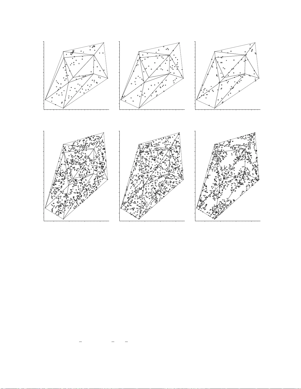
T ec hnical Rep ort # KU -EC-09-5: Relativ e Edge D ensit y of the U nderlying Graphs Based on Prop ortional-Edge Pro xim it y Catc h Digraphs for T esti ng Biv ariate Spatial P atterns Elv an Ceyhan ∗ No ve m b er 14, 2018 Abstract The use of data-rand om graphs in statistical testing of spatial p atterns is introdu ced recentl y . In this approac h, a random directed graph is constructed from the data u si ng the relative p ositions of the p oin ts from v arious classes. Diﬀerent random graphs result from diﬀerent deﬁnitions of the proximit y region asso ciated with eac h data p oin t and diﬀerent g raph statistics can b e emplo yed for patt ern testing. The approach used in t his article is based on underlying graphs of a family of data-random d ig raphs which is d etermined by a family of parameterized proximit y maps. The relative edge density of the AN D- and OR-u nderlying graphs is used as the summary statistic, pro viding an alternative t o the relativ e arc densit y and dominatio n n umber of the digraph emplo yed prev io usly . Properly scaled, relativ e ed g e d ensit y of the underlying graphs is a U -statistic, facilitating analytic study of its asymptotic distribution using standard U -statistic central limit theory . The approac h is illustrated with an application to the testing of biv ariate spatial clustering patterns of segregation and association. Knowl edge of the asymptotic distribution allo ws ev aluation of the Pitman asymptotic eﬃciency , hence selection of the proximit y map p ara m et er t o opt imize eﬃciency . Asymptotic eﬃciency and Mon te Carlo sim ulation analysis indicate that the AND-u nderlying version is better (in terms of pow er and eﬃciency) for the segregation alternativ e, while the OR-underlying version is better for the association alternative. The approach presented here is also val id for data in h ig her d imensi ons. Keywor ds: asso ci ation; asymptotic eﬃciency; clustering; complete spatial randomness; random graphs and digraphs; segregation; U - statis tic ∗ Address: Departmen t of Mathematics, Ko¸ c University , 34450 Sarıyer, Istanbul, T urkey . e-mai l: elceyhan@ku.edu.tr, tel:+90 (212) 338-1845 , fax: +90 (212) 338-1559. 1 1 In tro duction Classiﬁcation and clustering ha ve rece iv ed considera ble attention in the statistica l liter ature. In this ar ticle, a graph-ba sed approach for testing biv ar iate spa tial clus tering patterns is in tr oduced. The analysis of spatial point patterns in natura l p opulations has b een ex tensiv ely studied and have imp ortant implicatio ns in epidemio logy , po pulation biology , a nd eco logy . T he patterns of p oin ts from one class with resp ect to p oin ts fr om o ther classes, rather than the pattern o f p oin ts from o ne-class with res pect to the gro und , ar e in vestigated. The spatial relationships among t wo o r mor e classes hav e impor tan t implications esp ecially for plant sp ecies. See, for exa mple, Pielo u (196 1 ) and Dixon (1994, 2002). The go al of this article is to der iv e the as ymptotic distribution of the relative edge densit y of underlying graphs based on a particular digraph family and use it to test the spatial pattern of complete spatial randomness against spatial segr egation or asso ciation. Complete spatia l r andomness (CSR) is ro ughly deﬁned a s the lack of spatial interaction betw een the points in a given study area. Segregation is the pattern in which points of one class tend to cluster together, i.e., form one- class c lum ps. In asso ciation, the p oin ts of one clas s tend to o ccur more fr equen tly aro und p oints from the other class. F o r co n venience and generality , we call the diﬀerent t yp es of p oints “cla sses”, but the class can be repla ced by any characteristic of an o bserv a tion at a pa rticular lo cation. F o r example, the patter n o f s patial segr egation has b een inv estiga ted for pla n t sp ecies (Diggle 1 983), age c lasses of plants (Hamill and W rig h t (19 86)) a nd s exes o f dio ecious plants (Nanami et al. (1999)). In recent years, the use of mathematical gr aphs has als o gained p opularit y in spatial a nalysis (Rober ts et al. (2000)). In spatia l pattern analysis graph theore tic to ols pr o vide a w ay to mo ve be y ond E uclidean metr ics for spatial a nalysis. F or example, gr aph-based appr oac hes hav e b een prop osed to determine paths among ha bit ats at v ar ious scales and disp ersal mov ement distances, and bala nce data requirements with information conten t (F all et a l. (2007)). Although only re cen tly int ro duced to landscap e ecology , gra ph theory is well suited to ecologica l applications co ncerned with connec t ivity or mov ement (Minor and Urban (2007)). How ever, co n ven- tional graphs do no t explicitly maintain geogr aphic r eference, reducing utility of other geo -spatial informa tion. F all et al. (2007) int ro duce spatial graphs that in tegr ate a geometric r eference system that ties patc hes and paths to sp eciﬁc spa tial lo cations a nd spatial dimensions thereby pr eserving the re lev ant s patial infor mation. After a graph is constructed using spatial da ta, usually the sca le is lost (see for insta nce, Su et al. (20 07 )). Many con- cepts in spatial ecolog y depend on the idea of spatial a djacency which req uires information o n the close vicinity of an ob ject. Graph theory conv e nien tly ca n be used to express and communicate adjace ncy information allow- ing one to compute meaning f ul quantities related to spatial p oint pattern. Adding vertex and edge prop erties to graphs extends the problem doma in to netw ork mo deling (K eitt (2007)). W u and Murray (2008) pro pose a new measure based on g raph theory and spatial interaction, which reﬂects intra-patch and in ter-patch r elationships by quantifying co n tiguity w it hin patches and p oten tial contiguit y among patches. F riedman a nd Rafsky (1 983) also prop ose a gra ph-theoretic metho d to measure m ultiv ar iate as sociation, but their metho d is not designed to analy ze spatia l interaction b et ween tw o or mor e classes ; ins tead it is an extension of g eneralized corr elation co eﬃcien t (such a s Sp earman’s ρ or Kendall’s τ ) to measure multiv aria te (p ossibly nonlinear ) cor relation. A new type of spatial clustering test us ing directed graphs (i.e., digra phs) whic h is based on the rela tiv e po sitions o f the data points from v ar ious classes has also been develop ed recently . Data-rando m dig raphs are directed gr aphs in whic h eac h vertex corres ponds to a data p oint, a nd dir ected edge s (i.e., a rcs) are deﬁned in terms of some biv aria t e function on the da ta. F o r exa mple, nearest neighbor digraphs ar e deﬁned b y placing an ar c b et ween ea c h vertex and its nearest neig h b or. Prieb e et al. (200 1 ) introduced the class cover catch digraphs (CCCDs) in R and g a ve the ex act a nd the a symptotic distribution of the dominatio n num b er of the CCCDs. DeVinney et al. (20 02 ), Marchette a nd Prieb e (200 3) , Prieb e et al. (2003 a ), Prie be et al. (200 3b ), and DeVinney and Prieb e (2006) applied the concept in higher dimensions and demonstrated r elativ ely g oo d per formance o f CCCDs in clas siﬁcation. Their metho ds inv olve data r e duction (i.e., c ondensing ) by using approximate minimum dominating sets as pr ototyp e sets (since ﬁnding the exac t minim um dominating s et is an NP-hard problem in general — e.g., for CCCD in multiple dimensions — (see DeVinney and Pr iebe (2006)). F urthermor e the exact and the asymptotic distribution of the domination num b er of the CCCDs are not analytically tra ctable in multiple dimens ions. F or the domina tion num b er of CCCDs for one-dimensiona l data, a SLLN result is prov ed in DeVinney and Wierman (20 03), a nd this result is extended by Wierman and Xiang (2008); further more, a ge neralized SLLN result is provided by Wier man a nd Xiang (20 08 ), and a CL T is a lso prov ed by Xiang and Wier man (2009). The a symptotic dis tribution of the domina t ion n umber of CCCDs for non-uniform da ta in R is a lso calculated in a r ather gener al setting (Ceyhan (200 8 )). Ceyhan (20 05) generalized CCCDs to what is ca lled pr oximity c atch digr aphs (P CD s). The ﬁr st PCD family is in tro duced by Ceyhan a nd P riebe ( 2003); the parametrized v ers ion of this PCD is developed b y Ceyhan et al. (2007) where the 2 relative arc dens it y of the PCD is calculated a nd use d fo r spatial pa ttern analysis. Ceyhan and Prieb e (2005) int ro duced another digr aph family called pr op ortional e dge PCDs and calculated the asymptotic distribution of its domination num ber a nd used it for the same purp ose. The rela tiv e arc densit y of this PCD family is also c omputed and used in spatial pa tt ern analysis (Ceyhan et al. (2006)). Ceyhan and Prieb e (200 7 ) derived the a symptotic distr ibut ion of the domination num b er o f pr oportiona l-edge PC D s for tw o-dimensio nal unifor m data. The under lying g raphs based on digra phs ar e obta ined by replacing arcs in the digraph by edges based on biv ariate relations. If symmetric arcs are replaced b y edges, then we obtain the AND-underlying graph; and if all arcs a re replaced by edges without allowing mult i-edges, then we obtain the OR-underlying graph. The s tatistical to ol utilized in this article is the a symptotic theor y of U -sta t istics. Pro perly s caled, we demonstrate tha t the relative edge dens it y o f the underly ing gra phs of pro portional- edge PCDs is a U -statistic, which has asymptotic normality by the genera l central limit theory of U -statistics. F or the digraphs in tro duced by P riebe et a l. (20 01) , whose rela t ive arc density is also o f the U -statistic form, t he asymptotic mean and v ariance of the r elativ e density is not analytically tr actable, due to geometr ic diﬃculties encountered. How ever, for the PCDs intro duced in Ceyhan a nd P riebe (2003), Ceyhan et a l. (20 06), and Cey han et al. (2007), the relative ar c density h as tractable asymptotic mea n and v aria nce. W e deﬁne the underlying graphs of prop ortional-edge PCDs and their relative e dge dens it y in Section 2, provide the a symptotic distr ibut ion of the r elativ e edge density under the null hypo thesis in Section 3 .1 , and describ e the alter nativ es of segre gation and asso ciation in Section 3.2. W e prov e the consistency o f the relative edge dens it y in Section 4.1, and provide Pitman a symptotic eﬃciency in Sectio n 4.2. W e present the Monte Carlo simulation a nalysis for ﬁnite sa mple p erformance in Section 5, in par ticular, provide the Mo n te Carlo power analysis under se gregation in Section 5.1, and under a ssociation in Section 5.2. W e treat the m ultiple triangle cas e in Section 6, pr o vide extensio n to higher dimensions in Section 6.4. W e provide the discuss ion and conclusions in Section 7, and the tedio us ca lculations and long pro ofs are defer red to the App endix. 2 Relativ e Edge Densit y of Underlying Graphs 2.1 Preliminaries The main diﬀerence b et ween a g raph and a dig raph is that edges are directed in digr aphs, hence ar e called arc s. So the a rcs ar e denoted as ordere d pairs while edges are denoted as unorder ed pairs. The underlying gr aph of a digraph is the graph o btained by replacing ea c h arc uv ∈ A o r ea c h symmetric arc, { uv , v u } ⊂ A by the edg e ( u, v ). The former underlying gr aph will b e referred as the OR-underlying gr aph , while the latter a s the AND- underlying gr aph . Tha t is, the AND-underlying graph for dig raph D = ( V , A ) is the gr aph G and ( D ) = ( V , E and ) where E and is the set of edges suc h that ( u, v ) ∈ E and iﬀ uv ∈ A and v u ∈ A . The O R-underlying graph for D = ( V , A ) is the graph G or ( D ) = ( V , E or ) where E or is the set of edges suc h that ( u, v ) ∈ E or iﬀ uv ∈ A or v u ∈ A . The rela t ive edge density o f a gr aph G = ( V , E ) of order |V | = n , deno ted ρ ( G ), is deﬁned as ρ ( G ) = 2 |E | n ( n − 1 ) where | · | denotes the set cardina lit y function (Janso n et al. (2 000)). Th us ρ ( G ) repr esen ts the ratio of the nu m ber of edges in the graph G to the num b er o f e dges in the complete gr aph of or der n , which is n ( n − 1 ) / 2. Let (Ω , M ) b e a measura ble s pace and co nsider N : Ω → ℘ (Ω), where ℘ ( · ) repr esen ts the pow er set functional. Then g iv en Y m ⊂ Ω, the pr oximity map N Y ( · ) as sociates with eac h p oin t x ∈ Ω a pr oximity r e gion N Y ( x ) ⊆ Ω. The Γ 1 -region Γ 1 ( · , N ) : Ω → ℘ (Ω) asso ciates the regio n Γ 1 ( x, N Y ) := { z ∈ Ω : x ∈ N Y ( z ) } with ea c h p oin t x ∈ Ω. If X 1 , X 2 , . . . , X n are Ω-v alued random v ariables , then the N Y ( X i ) (and Γ 1 ( X i , N Y )), i = 1 , 2 , . . . , n ar e random s ets. If the X i are indep enden t and iden tically distributed, then so ar e the random sets N Y ( X i ) (and Γ 1 ( X i , N Y )). Consider the da t a-rando m P CD D with vertex set V = { X 1 , X 2 , . . . , X n } and arc set A deﬁned by X i X j ∈ A ⇐ ⇒ X j ∈ N Y ( X i ). The AND- u nderly ing gr aph , G and , o f D with the v ertex set V a nd the edge set E and is deﬁned by ( X i , X j ) ∈ E and iﬀ X i X j ∈ A and X j X i ∈ A . Likewise, the OR-u n de rlying gr aph , G or , o f D with the vertex set V and the edg e set E or is deﬁned by ( X i , X j ) ∈ E or ⇐ ⇒ X i X j ∈ A or X j X i ∈ A . Then ( X i , X j ) ∈ E and iﬀ X j ∈ N Y ( X i ) a nd X i ∈ N Y ( X j ) iﬀ X j ∈ N Y ( X i ) a nd X j ∈ Γ 1 ( X i , N Y ) iﬀ X j ∈ N Y ( X i ) ∩ Γ 1 ( X i , N Y ). 3 Similarly , ( X i , X j ) ∈ E or iﬀ X j ∈ N Y ( X i ) ∪ Γ 1 ( X i , N Y ). Since the random digra ph D dep ends on the (join t) distribution o f the X i and on the map N Y , so do the under lying graphs. The adjectiv e pr oximity — for the catch digr aph D and for the map N Y — co mes fro m thinking of the r egion N Y ( x ) a s r epresen ting thos e p oin ts in Ω “close” to x (T o ussain t (1980) and Jaro mczyk a nd T o ussain t (1992)). 2.2 Relativ e Edge Densit y of t he AND-Underlying Graphs The r elativ e edge density of G and ( D ), the AND-underlying gr aph bas ed on digraph D , is denoted a s ρ and ( D ). F or X i iid ∼ F , ρ and ( D ) is a U -statistic, ρ and ( D ) = 2 n ( n − 1 ) X X i 0. The asymptotic v ariance of ρ and n ( r ), 4 ν and ( r ), dep ends on only F and N r P E . Thus we need deter mine only µ and ( r ) a nd ν and ( r ) in or der to o btain the norma l appr o ximation ρ and n ( r ) approx ∼ N  µ and ( r ) , 4 ν and ( r ) n  . (6) The a bov e para graph holds fo r ρ or n ( r ) = ρ or ( X n ; h, N r P E ) a lso with ρ and n ( r ) is replac ed by ρ or n ( r ), h and 12 ( r ) a nd h and 13 ( r ) a re r eplaced by h or 12 and h or 13 , r espectively . F or r = 1, N r =1 P E ( x ) ∩ Γ r =1 1 ( x ) = ℓ ( v ( x ) , x ) which has zero R 2 -Leb esgue measure. Then we have E  ρ and n ( r = 1)  = E  h and 12 ( r = 1)  = µ and ( r = 1) = P ( X 2 ∈ N r =1 P E ( X 1 ) ∩ Γ r =1 1 ( X 1 )) = 0 . Similarly , P ( { X 2 , X 3 } ⊂ N r =1 P E ( X 1 ) ∩ Γ r =1 1 ( X 1 )) = 0. Thus, ν and ( r = 1) = 0. F urthermo re, for r = ∞ , N r = ∞ P E ( x ) ∩ Γ r = ∞ 1 ( x ) = T ( Y 3 ) fo r a ll x ∈ T ( Y 3 ) \ Y 3 . Then E  ρ and n ( r = ∞ )  = E  h and 12 ( r = ∞ )  = µ and ( r = ∞ ) = P ( X 2 ∈ N r = ∞ P E ( X 1 ) ∩ Γ r = ∞ 1 ( X 1 ) = P ( X 2 ∈ T ( Y 3 )) = 1. Similarly , P ( { X 2 , X 3 } ⊂ N r = ∞ P E ( X 1 ) ∩ Γ r = ∞ 1 ( X 1 )) = 1. Hence ν and ( r = ∞ ) = 0. Therefore, the CL T result in Eq uation (6) holds only for r ∈ (1 , ∞ ). F urthermore, ρ and n ( r = 1) = 0 a.s. and ρ and n ( r = ∞ ) = 1 a.s. F or r = 1, N r =1 P E ( x ) ∪ Γ r =1 1 ( x ) has p ositive R 2 -Leb esgue measure. Then P ( { X 2 , X 3 } ⊂ N r =1 P E ( X 1 ) ∪ Γ r =1 1 ( X 1 )) > 0. Th us, ν or ( r = 1 ) 6 = 0. On the other hand, for r = ∞ , N r = ∞ P E ( X 1 ) ∪ Γ r = ∞ 1 ( X 1 )) = T ( Y 3 ) for a ll X 1 ∈ T ( Y 3 ). T hen E [ ρ or n ( r = ∞ )] = E [ h or 12 ( r = ∞ )] = P ( X 2 ∈ N r = ∞ P E ( X 1 ) ∪ Γ r = ∞ 1 ( X 1 )) = µ or ( r = ∞ ) = P ( X 2 ∈ T ( Y 3 )) = 1. Similar ly , P ( { X 2 , X 3 } ⊂ N r = ∞ P E ( X 1 ) ∪ Γ r = ∞ 1 ( X 1 )) = 1. Hence ν or ( r = ∞ ) = 0. Ther efore, the CL T res ult fo r the OR-under lying ca se ho lds only for r ∈ [1 , ∞ ). Mor eo ver ρ or n ( r = ∞ ) = 1 a.s. R emark 2.2 . R elativ e Arc Density o f PCDs: The r elativ e arc density o f the digr aph D is deno ted as ρ ( D ). F or X i iid ∼ F , ρ ( D ) is als o shown to be a U -statistic (Ceyha n e t a l. (200 6 )), ρ ( D ) = 1 n ( n − 1) X X i 0. The ex plicit forms of asymptotic mean µ ( r ) a nd v ariance ν ( r ) are provided in Ceyha n et al. (2006).  3 Relativ e Edge Densit y under Null and A lternativ e P atterns 3.1 Null Distribution of Relativ e Edge Densit y The null hypothesis is generally some for m of c omplete sp atial r andomness ; thus we consider H o : X i iid ∼ U ( T ( Y 3 )) . If it is desired to have the sample size b e a random v ar iable, we may co nsider a spatial P o isson p oin t pro cess on T ( Y 3 ) a s our null hypothesis. W e ﬁrst pre sen t a “ geometry inv ariance” result whic h will simplify our subseq uen t analysis by a llo wing us to consider the sp ecial case o f the eq uilateral triangle . Let ρ and n ( r ) := ρ and ( n ; U ( T ( Y 3 )) , N r P E ) a nd ρ or n ( r ) := ρ or ( n ; U ( T ( Y 3 )) , N r P E ). 8 Theorem 3. 1 . Ge ometry Invari anc e: L et Y 3 = { y 1 , y 2 , y 3 } ⊂ R 2 b e thr e e non-c ol line ar p oints. F or i = 1 , 2 , . . . , n let X i iid ∼ F = U ( T ( Y 3 )) , the un i form distribution on the t ria ngle T ( Y 3 ) . Then for any r ∈ [1 , ∞ ] the distribution of ρ and n ( r ) and ρ or n ( r ) is indep endent of Y 3 , and henc e the ge ometry of T ( Y 3 ) . Pro of: A comp osition of transla tion, r otation, reﬂections, and sca ling will take any given triang le T o = T ( y 1 , y 2 , y 3 ) to the “basic” triang le T b = T ((0 , 0) , (1 , 0) , ( c 1 , c 2 )) with 0 < c 1 ≤ 1 2 , c 2 > 0 and (1 − c 1 ) 2 + c 2 2 ≤ 1, preserving unifo rmit y . The transforma tion φ : R 2 → R 2 given by φ ( u, v ) =  u + 1 − 2 c 1 √ 3 v , √ 3 2 c 2 v  takes T b to the equilateral tria ngle T e = T  (0 , 0) , (1 , 0) ,  1 / 2 , √ 3 / 2  . Inv e stigation of the Ja cobian sho ws that φ a lso preserves uniformity . F urthermore, the comp osition of φ with the rigid mo tion transformatio ns and s caling maps the bo undary of the original triang le T o to the b oundary of the equilater al tria ngle T e , the median lines of T o to the median lines o f T e , and lines para llel to the edges of T o to lines para llel to the edges of T e . Since the joint distribution of any c ollection of the h and ij ( r ) and h or ij ( r ) inv o lv es only proba bilit y conten t of unions and int ersections of regio ns bounded by pr ecisely such lines, and the pro babilit y conten t of such regio ns is pr eserv ed since uniformity is preser v ed, the desired result follows.  Based o n The orem 3.1, for our pro portional- edge pr o ximity map and the uniform n ull hypothesis, we may assume that T ( Y 3 ) is a s tandard equilateral triangle with Y 3 = { (0 , 0) , (1 , 0) , (1 / 2 , √ 3 / 2) } hencefor th. In the case o f this (prop ortional-edg e proximit y map, uniform nu ll hypothesis ) pair, the asymptotic null distribution of ρ and n ( r ) a nd ρ or n ( r ) a s a function of r can b e derived. Recall that µ and ( r ) = E  h and 12 ( r )  = P ( X 2 ∈ N r P E ( X 1 ) ∩ Γ r 1 ( X 1 )) = µ and ( r ) and µ or ( r ) = E [ h or 12 ] = P ( X 2 ∈ N r P E ( X 1 ) ∪ Γ r 1 ( X 1 )) = µ or ( r ) are the pro babilit y of a n edge o ccurring b et ween any tw o vertices in the AND- a nd OR-under lying g raphs, res pectively . Theorem 3.2. A s ymptotic Normality: F or r ∈ (1 , ∞ ) , √ n  ρ and n ( r ) − µ and ( r )  . p 4 ν and ( r ) L − → N (0 , 1) and for r ∈ [1 , ∞ ) , √ n ( ρ or n ( r ) − µ or ( r )) . p 4 ν or ( r ) L − → N (0 , 1) . where µ and ( r ) =            − 1 54 ( − 1+ r )(5 r 5 − 148 r 4 +245 r 3 − 178 r 2 − 232 r +128) r 2 ( r +2)( r +1) for r ∈ [1 , 4 / 3) , − 1 216 101 r 5 − 801 r 4 +1302 r 3 − 732 r 2 − 536 r +672 r ( r +2)( r +1) for r ∈ [4 / 3 , 3 / 2) , 1 8 r 8 − 13 r 7 +30 r 6 +148 r 5 − 448 r 4 +264 r 3 +288 r 2 − 368 r +96 r 4 ( r +2)( r +1) for r ∈ [3 / 2 , 2) , ( r 3 +3 r 2 − 2+2 r )( − 1+ r ) 2 r 4 ( r +1) for r ∈ [2 , ∞ ) , (8) µ or ( r ) =            47 r 6 − 195 r 5 +860 r 4 − 846 r 3 − 108 r 2 +720 r − 256 108 r 2 ( r +2)( r +1) for r ∈ [1 , 4 / 3) , 175 r 5 − 579 r 4 +1450 r 3 − 732 r 2 − 536 r +672 216 r ( r +2)( r +1) for r ∈ [4 / 3 , 3 / 2) , − 3 r 8 − 7 r 7 − 30 r 6 +84 r 5 − 264 r 4 +304 r 3 +144 r 2 − 368 r +96 8 r 4 ( r +1)( r +2) for r ∈ [3 / 2 , 2) , r 5 + r 4 − 6 r +2 r 4 ( r +1) for r ∈ [2 , ∞ ) , (9) ν and ( r ) = 11 X i =1 ϑ and i ( r ) I ( I i ) , (10) ν or ( r ) = 11 X i =1 ϑ or i ( r ) I ( I i ) (11) where ϑ and i ( r ) a nd ϑ or i ( r ) are provided in App endix Sectio ns 1 a nd 2, a nd the der iv ations o f µ and ( r ) and ν and ( r ) are pr o vided in App endix 3 , while those of µ or ( r ) a nd ν or ( r ) a re pr o vided in App endix 4 . Notice that µ and ( r = 1) = 0 and lim r →∞ µ and ( r ) = 1 (at rate O ( r − 1 )); and µ or ( r = 1) = 3 7 / 108 and lim r →∞ µ or ( r ) = 1 (at r ate O ( r − 1 )). T o illustr ate the limiting distribution, for example, r = 2 yields √ n ( ρ and n (2) − µ and (2)) p 4 ν and (2) = r 36288 0 n 58901  ρ and n (2) − 11 24  L − → N (0 , 1) 9 0 0.2 0.4 0.6 0.8 1 1 2 3 4 5 r µ and ( r ) µ ( r ) µ or ( r ) 0 0.05 0.1 0.15 0.2 1 2 3 4 5 r ν and ( r ) ν ( r ) ν or ( r ) Figure 3: Result of Theorem 3.2: asymptotic null means µ ( r ), µ and ( r ), and µ or ( r ) (left) and v ariances ν ( r ), 4 ν and ( r ), a nd 4 ν or ( r ) (right), from Equatio ns (8), (9), and (10) , (11), r espectively . Some v alues o f note: µ (1) = 37 / 21 6, µ and (1) = 0, a nd µ or (1) = 37 / 108, lim r →∞ µ ( r ) = lim r →∞ µ and ( r ) = lim r →∞ µ or ( r ) = 1, ν and ( r = 1 ) = 0 and lim r →∞ ν and ( r ) = 0, ν or ( r = 1) = 1 / 32 40 and lim r →∞ ν or ( r ) = 0, and ar gsup r ∈ [1 , ∞ ] ν ( r ) ≈ 2 . 045 with sup r ∈ [1 , ∞ ] ν ( r ) ≈ . 1 305, a rgsup r ∈ [1 , ∞ ] 4 ν and ( r ) ≈ 2 . 69 with sup r ∈ [1 , ∞ ] ν and ( r ) ≈ . 0 537, ar gsup r ∈ [1 , ∞ ] ν or ( r ) ≈ 1 . 765 with sup r ∈ [1 , ∞ ] ν or ( r ) ≈ . 0318 . and √ n ( ρ or n (2) − µ or (2)) p 4 ν or (2) = r 12096 0 n 13189  ρ or n (2) − 19 24  L − → N (0 , 1) or eq uiv alently , ρ and n (2) approx ∼ N  11 24 , 58901 36288 0 n  and ρ or n (2) approx ∼ N  19 24 , 13189 12096 0 n  . By construction of the underlying g raphs, there is a natural o rdering o f the means of r elativ e ar c and edge densities. Lemma 3.3. The me ans of the r elative e dge densities and ar c density have the fol lowing or dering: µ and ( r ) < µ ( r ) < µ or ( r ) for all r ∈ [1 , ∞ ) . F urthermor e, for r = ∞ we have µ and ( r ) = µ ( r ) = µ or ( r ) = 1 . Pro of: Recall that µ and ( r ) = E [ ρ and n ( r )] = P ( X 2 ∈ N r P E ( X 1 ) ∩ Γ r 1 ( X 1 )), µ ( r ) = E [ ρ n ( r )] = P ( X 2 ∈ N r P E ( X 1 )), and µ or ( r ) = E [ ρ or n ( r )] = P ( X 2 ∈ N r P E ( X 1 ) ∪ Γ r 1 ( X 1 )). And N r P E ( X 1 ) ∩ Γ r 1 ( X 1 ) ⊆ N r P E ( X 1 ) ⊆ N r P E ( X 1 ) ∪ Γ r 1 ( X 1 ) with probability 1 for all r ≥ 1 with e qualit y holding for r = ∞ only . Then the des ired result follows. See also Figure 3.  Note that the above lemma ho lds for all X i that has a contin uous distribution o n T ( Y 3 ). There is also a sto c hastic order ing for the relative edg e and ar c densities a s follows. Theorem 3.4. F or su ﬃci en tly s m a l l r , ρ and n ( r ) < S T ρ n ( r ) < S T ρ or n ( r ) as n → ∞ . Pro of: Ab o ve we have proved that µ and ( r ) < µ ( r ) < µ or ( r ) for all r ∈ [1 , ∞ ). F or s mall r ( r ≤ b r ≈ 1 . 8 ) the asymptotic v aria nces hav e the same order ing, 4 ν and ( r ) < ν ( r ) < 4 ν or ( r ). Since ρ and n ( r ) , ρ n ( r ) , ρ or n ( r ) are asymptotically normal, then the desired result follows. See a lso Fig ure 3.  Figures 4 and 5 indicate that, for r = 2, the no rmal approximation is acc urate even for small n although kurtosis ma y be indicated for n = 10 in the AND-underlying case, and skewness may b e indica t ed for n = 1 0 in the OR-underlying c ase. Figur es 6 and 7 demonstr ate, how ever, that s ev ere skewness obtains for some v alues of n , r . The ﬁnite sample v ar iance and skewness ma y be derived ana lytically in muc h the same wa y as was 4 ν and ( r ) (and 4 ν or ( r )]) for the asymptotic v ar iance. In fact, the exact distribution o f ρ and n ( r ) (and ρ or n ( r )) is, in principle, av a ilable by succes siv ely conditioning on the v alue s of the X i . Alas, while the joint distribution of h and 12 ( r ) , h and 13 ( r ) (a nd h or 12 ( r ) , h or 13 ( r )) is av a ilable, the joint dis tribution of { h and ij ( r ) } 1 ≤ i 1 , γ or n ( r ) < S T γ n ( r ) < S T γ and n ( r ) . Pro of: F o r all x ∈ T ( Y 3 ), we hav e N r P E ( x ) ∩ Γ r 1 ( x ) ⊆ N r P E ( x ) ⊆ N r P E ( x ) ∪ Γ r 1 ( x ). F or X ∼ U ( T ( Y 3 )), we ha ve N r P E ( X ) ∩ Γ r 1 ( X ) ( N r P E ( X ) ( N r P E ( X ) ∪ Γ r 1 ( X ) a.s. Moreov er, γ n ( r ) = 1 iﬀ X n ⊂ N r P E ( X i ) fo r some i ; γ and n ( r ) = 1 iﬀ X n ⊂ N r P E ( X i ) ∩ Γ r 1 ( X i ) for some i ; and γ or n ( r ) = 1 iﬀ X n ⊂ N r P E ( X i ) ∪ Γ r 1 ( X i ) fo r some i . So it fo llo ws that P ( γ and n ( r ) = 1) < P ( γ n ( r ) = 1) < P ( γ or n ( r ) = 1). In a similar fashion, we hav e P ( γ and n ( r ) ≤ 2) < P ( γ n ( r ) ≤ 2) < P ( γ or n ( r ) ≤ 2). Since P ( γ n ( r ) ≤ 3) = 1 (Ceyhan and Prieb e (2005)), it follows that P ( γ or n ( r ) ≤ 3) = 1 als o ho lds as P ( γ n ( r ) ≤ 3) < P ( γ or n ( r ) ≤ 3). Hence the desired sto c hastic ordering follows.  Note the sto chastic orde ring in the ab ov e theorem holds for any con tin uous distribution F with supp ort being in T ( Y 3 ). 3.2 Alternativ es: Segregation and Asso ciation The phenomenon known a s se gr e gation in volv es observ ations fro m diﬀerent classe s having a tendency to r epel each other — in our cas e, this means the X i tend to fall awa y from all elements of Y 3 . Asso ciation inv olves observ ations fr om diﬀerent cla sses having a tendency to attract one another, so tha t the X i tend to fall nea r an element o f Y 3 . See, for insta nce, Dixon (199 4 ) and C oomes et a l. (199 9) . 11 0.00 0.05 0.10 0.15 0.20 0.25 0.30 0 5 10 15 20 P S f r a g r e p la c e m e n t s density 0.3 0.4 0.5 0.6 0.7 0.8 0.9 1.0 0 2 4 6 8 P S f r a g r e p la c e m e n t s density Figure 6: Depicted a re the histog rams for 10000 Monte Ca rlo replica tes of ρ and 10 (1 . 05) (left) a nd ρ and 10 (5) (r igh t) indicating s ev ere s mall sample skewness for ex t reme v alues of r . Notice that the vertical axes are diﬀerently scaled. 0.2 0.3 0.4 0.5 0.6 0.7 0.8 0.9 0 1 2 3 4 5 6 P S f r a g r e p la c e m e n t s density 0.80 0.85 0.90 0.95 1.00 0 10 20 30 40 P S f r a g r e p la c e m e n t s density Figure 7: Depicted a re the histog rams for 1 0000 Monte Car lo r eplicates of ρ or 10 (1) (left) and ρ or 10 (5) (right) indicating s ev ere s mall sample skewness for ex t reme v alues of r . Notice that the vertical axes are diﬀerently scaled. W e deﬁne tw o simple clas ses o f alternativ e s, H S ε and H A ε with ε ∈  0 , √ 3 / 3  , for segr egation and asso ciation, resp ectiv ely . F or y ∈ Y 3 , let e ( y ) denote the edge o f T ( Y 3 ) o pposite vertex y , and for x ∈ T ( Y 3 ) let ℓ y ( x ) denote the line parallel to e ( y ) thro ugh x . Then deﬁne T ( y , ε ) = { x ∈ T ( Y 3 ) : d ( y , ℓ y ( x )) ≤ ε } . Let H S ε be the mo del under which X i iid ∼ U ( T ( Y 3 ) \ ∪ y ∈Y 3 T ( y , ε )) and H A ε be the mo del under which X i iid ∼ U ( ∪ y ∈Y 3 T ( y , √ 3 / 3 − ε )). Thu s the s egregation mo del excludes the p ossibilit y of an y X i o ccurring near a y j , and the asso ciation mo del requires that a ll X i o ccur near a y j . The √ 3 / 3 − ε in the deﬁnition of the ass ociation alternative is so that ε = 0 yields H o under b oth clas ses o f a lternativ es . R emark 3.6 . These deﬁnitions of the alternatives ar e given fo r the standard equila teral triang le. The g eometry inv ariance result of Theor em 3 .1 still holds under the alternatives H S ε and H A ε . In particula r, the segregatio n alternative with ε ∈  0 , √ 3 / 4  in the standard equilater al tria ngle corr esponds to the ca se that in an arbitra ry triangle, δ × 100% o f the ar ea is carved awa y a s for bidden from the vertices using line segments para llel to the opp osite edge where δ = 4 ε 2 (whic h implies δ ∈ (0 , 3 / 4)). B ut the segr egation alterna t ive with ε ∈  √ 3 / 4 , √ 3 / 3  in the standard equilatera l tria ngle cor responds to the case that in an arbitra ry tria ngle, δ × 100% of the area is carved a way as forbidden around the vertices using line segments pa rallel to the o pposite edge where δ = 1 − 4  1 − √ 3 ε  2 (whic h implies δ ∈ (3 / 4 , 1)). This argument is for the seg regation alterna tiv e; a simila r construction is av ailable for the asso ciation alternative.  The asymptotic normality of the rela tiv e e dge density under the alternatives follows as in the null ca se. Theorem 3.7. Asymptotic Normality under the Alternatives: L et µ and ( r , ε ) b e the m e an and ν and ( r , ε ) b e the varianc e of ρ and n ( r ) un d er the alternatives for r ∈ [1 , ∞ ) and ε ∈  0 , √ 3 / 3  . Then under H S ε and H A ε , 12 √ n ( ρ and n ( r ) − µ and ( r , ε )) L − → N (0 , 4 ν and ( r , ε )) for the values of the p air ( r, ε ) for which ν and ( r , ε ) > 0 . A similar r esult holds for ρ or n ( r ) . Pro of: Under the alternatives, i.e., ε > 0 , ρ and n ( r ) is a U -statistic with the same s ymmetric kernel h and ij ( r ) as in the null case. Let E ε [ · ] b e the exp ectation with resp ect to the uniform distribution under the alternatives with ε ∈  0 , √ 3 / 3  . The mean µ and ( r , ε ) = E ε  ρ and n ( r )  = E ε  h and 12 ( r )  , now a function o f both r and ε , is ag ain in [0 , 1 ]. T he asymptotic v ariance, 4 ν and ( r , ε ) = 4 Cov  h and 12 ( r ) , h and 13 ( r )  , also a function o f both r and ε , is bo unded above b y 1 / 4, as befo re. Thus asymptotic nor malit y obtains provided ν and ( r , ε ) > 0; otherwise ρ and n ( r ) is degenerate. The n under H S ε , ν and ( r , ε ) > 0 for ( r , ε ) in (1 , √ 3 / (2 ε )) × (0 , √ 3 / 4] or (1 , √ 3 /ε − 2) × ( √ 3 / 4 , √ 3 / 3), and under H A ε , ν and ( r , ε ) > 0 for ( r , ε ) in (1 , ∞ ) ×  0 , √ 3 / 3  . Also under H S ε , ν or ( r , ε ) > 0 for ( r , ε ) in [1 , √ 3 / (2 ε )) × (0 , √ 3 / 4] o r [1 , √ 3 /ε − 2 ) × ( √ 3 / 4 , √ 3 / 3), and under H A ε , ν or ( r , ε ) > 0 for ( r , ε ) in (1 , ∞ ) ×  0 , √ 3 / 3  or { 1 } × (0 , √ 3 / 12).  Notice that for the asso ciation class of alter nativ es any r ∈ (1 , ∞ ) yields asymptotic no rmalit y for all ε ∈  0 , √ 3 / 3  in b oth AND- and OR-underlying cases , while for the seg regation class of alternatives o nly r = 1 yields this universal a symptotic norma lit y in the OR-under lying case, and such an ε do es not exist fo r the AND-underlying case. The rela tiv e edge density of the underly ing g raphs based on the PCD is a test statistic for the s egrega- tion/asso ciation alternative; r ejecting for extreme v alues of ρ and n ( r ) is a ppropriate since under segrega t ion w e exp ect ρ and n ( r ) to b e large, while under a ssocia t ion we e xpect ρ and n ( r ) to b e small. The same holds for ρ or n ( r ). Using the test statistics R and n ( r ) = √ n  ρ and n ( r ) − µ and ( r )  . p 4 ν and ( r ) , and R or n ( r ) = √ n ( ρ or n ( r ) − µ or ( r )) . p 4 ν or ( r ) (12) for AND- and OR-under lying cases, resp ectively , the asymptotic critica l v alue for the one-s ided level α test against seg regation is given by z α = Φ − 1 (1 − α ) (13) where Φ( · ) is the standa rd no rmal dis t ribution function. The test rejects for R and n ( r ) > z α against seg regation. Against as sociation, the test rejects for R and n ( r ) < z 1 − α . The same holds for the tes t s tatistic R or n ( r ). 4 Asymptotic P erformance of Relativ e Edge Densit y 4.1 Consistency Theorem 4.1. The test against H S ε which r eje cts for R and n ( r ) > z α and the test against H A ε which r eje cts for R and n ( r ) < z 1 − α ar e c onsist en t for r ∈ (1 , ∞ ) and ε ∈  0 , √ 3 / 3  . The same holds for R or n ( r ) with r ∈ [1 , ∞ ) . Pro of: Since the v aria nce of the asymptotically norma l test statistic, under b oth the null and the alternatives, conv erg es to 0 as n → ∞ (or might be zero for n < ∞ ), it remains to s ho w that the mean under the null, µ and ( r ) = E  ρ and n ( r )  , is less than (gr eater than) the mean under the alternative, µ and ( r , ε ) = E  ρ and n ( r )  against segreg ation (asso ciation) for ε > 0 . Whence it will fo llo w that p o w er conv erg es to 1 as n → ∞ . Let P ε ( · ) be the probability with resp ect to the uniform distribution under the alterna t ives with ε ∈  0 , √ 3 / 3  . Then against seg regation, we hav e µ and ( r ) = P 0 ( X 2 ∈ N r P E ( X 1 ) ∩ Γ r 1 ( X 1 )) = P 0 ( X 2 ∈ N r P E ( X 1 ) ∩ Γ r 1 ( X 1 ) , X 1 ∈ ∪ y ∈Y 3 T ( y , ε )) + P 0 ( X 2 ∈ N r P E ( X 1 ) ∩ Γ r 1 ( X 1 ) , X 1 ∈ T ( Y 3 ) \ ∪ y ∈Y 3 T ( y , ε )) = P 0 ( X 2 ∈ N r P E ( X 1 ) ∩ Γ r 1 ( X 1 ) | X 1 ∈ ∪ y ∈Y 3 T ( y , ε )) P 0 ( X 1 ∈ ∪ y ∈Y 3 T ( y , ε )) + P 0 ( X 2 ∈ N r P E ( X 1 ) | X 1 ∈ T ( Y 3 ) \ ∪ y ∈Y 3 T ( y , ε )) P 0 ( X 1 ∈ T ( Y 3 ) \ ∪ y ∈Y 3 T ( y , ε )) < P 0 ( X 2 ∈ N r P E ( X 1 ) ∩ Γ r 1 ( X 1 ) | X 1 ∈ ∪ y ∈Y 3 T ( y , ε )) p 1 + P ε ( X 2 ∈ N r P E ( X 1 ) ∩ Γ r 1 ( X 1 ) | X 1 ∈ T ( Y 3 ) \ ∪ y ∈Y 3 T ( y , ε )) p 2 = E 0 ( I ( X 2 ∈ N r P E ( X 1 ) ∩ Γ r 1 ( X 1 )) | X 1 ∈ ∪ y ∈Y 3 T ( y , ε )) p 1 + E ε ( I ( X 2 ∈ N r P E ( X 1 ) ∩ Γ r 1 ( X 1 )) | X 1 ∈ T ( Y 3 ) \ ∪ y ∈Y 3 T ( y , ε )) p 2 where p 1 = P 0 ( X 1 ∈ ∪ y ∈Y 3 T ( y , ε )) a nd p 2 = P 0 ( X 1 ∈ T ( Y 3 ) \ ∪ y ∈Y 3 T ( y , ε )) = 1 − p 1 . Then µ and ( r , ε ) > µ and ( r ) (1 − p 1 ) p 2 = µ and ( r ) . Likewise, we hav e µ and ( r , ε ) = E ε  ρ and n ( r )  < E [ ρ n ( r )] = µ and ( r ), for asso ciation. The consis t ency follows for the OR-underlying ca se in a similar fashion.  13 4.2 Pitman Asymptotic E ﬃcien cy Pitman asymptotic eﬃciency (P AE) pro vides an in vestigation of “loca l asymptotic power” — local ab out H o . This inv o lv es the limit as ε → 0 as well as the limit a s n → ∞ . A detailed discuss ion of P AE can b e found in Kendall a nd Stuart (19 79 ) a nd Eeden (1963). F o r segreg ation or ass ociation a lternativ es with the AND- underlying graphs, the P AE is giv en b y  ( µ and ) ( k ) ( r , ε = 0)  2 ν and ( r ) where ( µ and ) ( k ) ( r , ε = 0) is the k th deriv ative with resp ect to ε so that ( µ and ) ( k ) ( r , ε = 0) 6 = 0 but ( µ and ) ( k − 1) ( r , ε = 0) = 0 for k = 1 , 2 , . . . . Lik ewise the sa me holds for the OR-underlying case. Then under segregation alternative H S ε , the P AE is given by P AE S and ( r ) = (( µ and ) ′′ ( r , ε = 0)) 2 ν and ( r ) and P AE S or ( r ) = (( µ or ) ′′ ( r , ε = 0)) 2 ν or ( r ) since ( µ and ) ′ ( r , ε = 0) = 0 and ( µ or ) ′ ( r , ε = 0) = 0. Under asso ciation alterna tiv e H A ε is P AE A and ( r ) = (( µ and ) ′′ ( r , ε = 0)) 2 ν and ( r ) and P AE A or ( r ) = (( µ or ) ′′ ( r , ε = 0)) 2 ν or ( r ) since ( µ and ) ′ ( r , ε = 0) = ( µ or ) ′ ( r , ε = 0) = 0. E quations (10) and (11) provide th e denominato rs; the n umerators require a bit of additional work, but µ and ( r , ε ) and µ or ( r , ε ) are a v ailable for small eno ugh ε , whic h is all we need here. See App endix 5 for explicit forms of µ and ( r , ε ) and µ or ( r , ε ) for s egregation and asso ciation, and the deriv ations of µ and ( r , ε ) and µ or ( r , ε ) ar e provided in App endix 6. Let P AE S ( r ) and P AE A ( r ) denote the P AE score against the segre gation and a ssocia tion alter nativ es, resp ectiv ely , for the relative ar c density of the PCD ba sed o n N r P E (see Ceyha n et al. (2006) mo re detail). Figure 8 presents the P AE as a function of r for b oth seg regation and asso ciation in the dig raph, AND, and OR- underlying gra ph cases. F or large n and small ε , P AE a nalysis sugg ests choos ing r lar ge for test- ing against se gregation in all three cases and choo sing r sma ll fo r testing against asso ciation, a rbitrarily close to 1 for the AND- and OR-underly ing cases , but around 1.1 for the digra ph case. F urthermor e, in segrega - tion, P AE S or ( r ) < P AE S ( r ) < P AE S and ( r ), sugg esting the use of AND-underlying version. Under asso ciation, max  P AE S and ( r ) , P AE S ( r ) < P AE S or ( r )  implying the use of O R-underlying version. 0 200 400 600 800 1000 1 1.5 2 2.5 3 3.5 4 r P AE S and ( r ) P AE S ( r ) P AE S or ( r ) 0 5000 10000 15000 1 1.5 2 2.5 3 3.5 4 r P AE A or ( r ) P AE A and ( r ) P AE A ( r ) Figure 8: P itman asymptotic eﬃciency against segr egation (left) and asso ciation (right) as a function of r . Some v alues of note: P AE S ( r = 1) = 160 / 7, P AE S and ( r = 1) = 4000 / 17, P AE S or ( r = 1) = 160 / 9, lim r →∞ P AE S ( r ) = lim r →∞ P AE S and ( r ) = lim r →∞ P AE S or ( r ) = ∞ , and P AE S and ( r ) ha s a lo cal supremum a t ≈ 1 . 35. Also P AE A ( r = 1) = 0, P AE A and ( r = 1) = P AE A or ( r = 1 ) = ∞ , lim r →∞ P AE A ( r ) = lim r →∞ P AE A and ( r ) = lim r →∞ P AE A and ( r ) = 0, argsup r ∈ [1 , ∞ ] P AE A ( r ) ≈ 1 . 1, and P AE A and ( r ) ha s a lo cal supremum at r = 1 . 5 a nd a lo cal inﬁmum at r ≈ 1 . 2 R emark 4.2 . Ho dges-Lehmann Asymptotic Eﬃ ciency: Ho dges-Lehmann asymptotic eﬃciency (HLAE) (Hodg es a nd L ehmann (195 6) ) is given by HLAE( ρ and n ( r ) , ε ) := ( µ and ( r , ε ) − µ and ( r )) 2 ν and ( r , ε ) . 14 Unlik e P AE, HLAE do es no t inv olve the limit as ε → 0. Since this r equires the mean and, esp ecially , the asymptotic v a riance of ρ and n ( r ) un d er t h e alternative , we a void the ex plicit inv estigatio n of HLAE. HLAE for OR-underlying g raphs can b e deﬁned simila rly . The o rdering of HLAE seems to b e the same as that of P AE.  R emark 4.3 . Asymptotic P ow er F unction Analysis: The asymptotic p ow er function (Kendall a nd Stuar t (1979)) allo ws in vestigation of pow er as a function of r , n , and ε using the asymptotic critical v alue and a n app eal to norma lit y . Under a sp eciﬁc se gregation alternative H S ε , the asymptotic p o wer function for AND-underlying graphs is given by Π S and ( r , n, ε ) = 1 − Φ z α p ν and ( r ) p ν and ( r , ε ) + √ n ( µ and ( r ) − µ and ( r , ε )) p ν and ( r , ε ) ! . Under H A ε , we hav e Π A and ( r , n, ε ) = Φ z 1 − α p ν and ( r ) p ν and ( r , ε ) + √ n ( µ and ( r ) − µ and ( r , ε )) p ν and ( r , ε ) ! . F or OR-under lying g raphs, the asymptotic p o wer functions, Π S or ( r , n, ε ) a nd Π A or ( r , n, ε ), are deﬁned similar ly . How ever it is not inv estigated in this article.  5 Mon te Carlo Sim ulation Analysis for Finite Sample P erformance W e implement the Monte Carlo simulations under the ab ov e describ ed n ull and alter nativ es for r ∈ { 1 , 11 / 10 , 6 / 5 , 4 / 3 , √ 2 , 3 / 2 , 2 , 3 , 5 } . 5.1 Mon te Carlo Po w er Analysis under Segregation In Figur e 9, w e presen t a Monte Carlo investigation ag ainst the s egregation a lternativ e H S √ 3 / 8 for r = 1 . 1 and n = 10 (left) a nd n = 100 (right). The empirical p o wer estimates are calculated based on the Mont e Carlo critical v alues. Le t b β S mc  ρ and n ( r )  and b β S mc ( ρ or n ( r )) s t and for the co rrespo nding empirical p ow er estimates fo r the AND- and OR-underly ing cases. With n = 10, the null and alterna tiv e pr obabilit y density functions for ρ and 10 (1 . 1) and ρ or 10 (1 . 1) ar e very similar, implying small p ow er (10,0 00 Mon te Ca rlo replicates yie ld empirica l pow e r v alues b β S mc  ρ and 10  = 0 . 1 318 a nd b β S mc ( ρ or 10 ) = 0 . 05 39). Among the 1 0000 Monte Carlo replicates under H o , we ﬁnd the 95 th per cen tile v alue and use it as the Mo n te Ca rlo critical v alue at . 05 level for the segre gation alternativ e, and use 5 th per cen tile v a lue for the asso ciation alternative. With n = 100, there is more separa tion b et ween n ull and alternative pro babilit y density functions in the underlying case s where s eparation is muc h less emphasized in the OR-underlying c ase; 1 000 Mo n te Car lo r eplicates yield b β S mc  ρ and 100  = 0 . 994 and b β S mc ( ρ or 100 ) = 0 . 298 where the empir ical power estimates a re based o n Monte Carlo critical v a lues. Notice also that the pr obabilit y density functions are s k ewed rig h t for n = 10 in b oth underlying cases , while approximate no rmalit y holds for n = 100. F or a given alter nativ e and sample size we ma y consider optimizing the empirica l p o wer o f the test a s a function o f the proximity factor r . Figure 10 presents a Monte Ca rlo inv e stigation of empirica l p o wer bas ed on Monte Carlo critical v alues agains t H S √ 3 / 8 and H S √ 3 / 4 as a function of r for n = 10 with 1000 r eplicates. The corres ponding empirical p ow er estimates are given in T able 1. Our Mon te Carlo estimates of r ∗ ε , the v alue of r whic h ma ximizes the p o wer a gainst H S ε , are r ∗ √ 3 / 8 = 3 a nd r ∗ √ 3 / 4 ∈ [4 / 3 , 3] in the AND-underlying ca se, and r ∗ √ 3 / 8 = 2 and r ∗ √ 3 / 4 ∈ [4 / 3 , 2] in the OR-underlying case. That is, more se v ere seg regation (larg er ε ) sugge sts a smaller choice of r in b oth cases . F or b oth ε v alues, smaller r v alues a re sugg ested in the O R-underlying ca se compared to the AND-underlying case . F or a given a lt ernative and sample size we may consider analyzing the p o wer of the test — using the asymptotic critical v alue— as a function of the proximity facto r r . Let b α n ( r ) denote the e mpirical signiﬁca nce levels and b β n ( r ) empirical power estimates bas ed on the asymptotic critica l v alue. Figure 11 pr esen ts a Mon te Carlo in vestigation of empirical p o wer based on asymptotic critical v alue a gainst H S √ 3 / 8 and H S √ 3 / 4 as a function of r for n = 10. The corresp onding empirical p o wer estimates are g iv en in T able 2. In the AND-underlying case, the empirical signiﬁcance level, b α n =10 ( r ), is closes t to . 05 for r = 2 and 3 which hav e the empirica l p o wer b β 10 (2) = . 3846 and b β 10 (3) = . 5767 for ε = √ 3 / 8, and b β 10 (2) = b β 10 (3) = 1 for ε = √ 3 / 4. In the OR-underlying 15 −0.05 0.00 0.05 0.10 0.15 0.20 0.25 0 2 4 6 8 10 12 P S f r a g r e p la c e m e n t s kernel density estimate relative edge density 0.04 0.06 0.08 0.10 0 10 20 30 40 50 60 70 P S f r a g r e p la c e m e n t s kernel density estimate relative edge density 0.2 0.3 0.4 0.5 0.6 0.7 0.8 0 1 2 3 4 5 6 7 P S f r a g r e p la c e m e n t s kernel density estimate relative edge density 0.32 0.34 0.36 0.38 0.40 0.42 0.44 0 10 20 30 P S f r a g r e p la c e m e n t s kernel density estimate relative edge density Figure 9: Tw o Monte Carlo exper imen ts against the segreg ation alternatives H S √ 3 / 8 . Depicted are kernel density estimates of ρ and n (1 . 1) for n = 10 (top left) and n = 10 0 (top right) and ρ or n (1 . 1) for n = 10 (bottom left) and n = 100 (b ottom right) under the null (solid) and a lternativ e (dashed) cases. case, the empiric al sig niﬁcance le v el, b α n =10 ( r ), is c losest to . 05 for r = 2 —larger for a ll r v a lues — which hav e the e mp irical p o w er b β 10 (2) = . 159 4 for ε = √ 3 / 8, and b β 10 (2) = 1 for ε = √ 3 / 4. So, for small sample sizes, mo derate v alues of r is more a ppropriate for normal appr o ximation, as they yield the desired sig niﬁcance level, and the mor e se v ere the segr egation, hig her the p o wer es tim ate. F ur thermore, the AND-underly ing version seems to p erform b etter than the OR-underlying version fo r se gregation alter nativ es. 5.2 Mon te Carlo Po w er Analysis under Asso ciation In Fig ure 12, we pr esen t a Monte Car lo inv estigatio n against the asso ciation alter nativ e H A √ 3 / 12 for r = 1 . 1 and n = 10 (left) a nd n = 100 (right). The empirical p o wer estimates are calculated based on the Mont e Carlo critical v alues Let b β A mc  ρ and n ( r )  and b β A mc ( ρ or n ( r )) stand for the cor responding empirical p o wer estimates for the AND- and OR-underly ing cases. As ab o ve, with n = 1 0, the n ull and alter nativ e probability density functions for ρ and 10 (1 . 1) and ρ or 10 (1 . 1) are very similar , implying small pow er— in fact, virtually no p o wer— (10,00 0 Mon te Carlo replicates yield the following empir ical p o wer estimates based on Monte Carlo critical v alues: b β A mc  ρ and 10  = 0 . 0 and b β A mc ( ρ or 10 ) = 0 . 0). With n = 100, there is mor e separa tion b et ween null and alter nativ e proba bilit y density functions in the under lying cases where separatio n is muc h les s emphasized in the AND-underlying ca se; for this case, 1000 Monte Carlo r eplicates yield the following empirical pow er estimates based on Monte Carlo critical v alues: b β A mc  ρ and 100  = 0 . 0 09 and b β A mc ( ρ or 100 ) = 0 . 939 . Notice also that the probability density functions are skew ed right f or n = 10 in b oth underlying cases, with mor e skewness in OR-underlying case, while approximate 16 1.0 1.5 2.0 2.5 3.0 0.0 0.2 0.4 0.6 0.8 1.0 P S f r a g r e p la c e m e n t s power r 1.0 1.5 2.0 2.5 3.0 0.3 0.4 0.5 0.6 0.7 0.8 0.9 1.0 P S f r a g r e p la c e m e n t s power r 1.0 1.5 2.0 2.5 3.0 0.0 0.2 0.4 0.6 0.8 1.0 P S f r a g r e p la c e m e n t s power r 1.0 1.5 2.0 2.5 3.0 0.0 0.2 0.4 0.6 0.8 1.0 P S f r a g r e p la c e m e n t s power r Figure 10: Empiric al p ow er estimates based on Mon te Carlo critical v alues as a function of r against segreg ation alternatives with the AND-underlying ca se (top tw o) and OR-underly ing case (bo ttom tw o); in b oth cases , we hav e H S √ 3 / 8 (left) a nd H S √ 3 / 4 (right) for n = 10 and N mc = 1000 Monte Carlo r eplicates. normality holds for n = 100 for b oth cas es. In Fig ure 1 3 , we a lso pr esen t a Mo n te Ca rlo inv estigatio n of empirical p ow er based o n Mo n te Carlo critical v alues a gainst H A √ 3 / 12 and H A 5 √ 3 / 24 as a function o f r for n = 10 with 10 00 replicates. The corre sponding empirical p o w er estimates a re prese n ted in T able 3. Our Monte Car lo estimates o f r ∗ ε are r ∗ √ 3 / 12 = 2 a nd r ∗ 5 √ 3 / 24 = 3 in b oth under lying cases . That is, more severe a ssocia t ion (lar ger ε ) sug gests a lar ger choice of r in bo th c ases. In Figure 1 4 , we present a Monte Ca rlo inv es tigation o f p o wer ba sed on asympto t ic cr itical v alues against H A √ 3 / 12 and H A 5 √ 3 / 24 as a function o f r for n = 10. In the AND-underlying case, the empirical sig niﬁcance level, b α n =10 ( r ), is a bout . 05 for r = 2 and 3 which ha ve the empirical p o wer b β 10 (2) ≈ . 2 with maximum power at r = 2 for ε = √ 3 / 12, and b β 10 (3) = 1 for ε = 5 √ 3 / 24. In the OR-underlying case, the empirical signiﬁcance level, b α n =10 ( r ), is closest to . 05 for r = 1 . 5 which hav e the empirical p o wer b β 10 (1 . 5) ≈ . 45 for ε = √ 3 / 12, and b β 10 (1 . 5) = 1 for ε = 5 √ 3 / 24. So, for small sample sizes, mo derate v alues of r is more appro priate for normal approximation, a s they yield the desired signiﬁcance level, and the more severe the a ssocia tion, higher the power estimate. F ur th ermore, the OR- underlying v ers ion seems to p erform better tha n t he AND-underlying version for ass ociation alternatives. The empirical signiﬁcance levels, and empir ical p ow er b β S n ( r , ε ) v alues based on asy mpt otic critica l v alues under H A ε for ε = √ 3 / 12 , 5 √ 3 / 24 are given in T able 4. 17 n = 10 and N mc = 1000 AND-underlying ca se r 1 1 1/10 6/ 5 4/3 √ 2 3/2 2 3 b C S mc 0 . 0 ¯ 2 0 . ¯ 1 .2 0 . 2 ¯ 8 0 . 3 ¯ 5 0 . 4 ¯ 2 0 . 7 ¯ 3 0 . 9 ¯ 7 b α S mc ( n ) 0.023 0 .048 0.035 0.044 0.040 0.036 0.031 0.039 b β S mc ( √ 3 / 8) 0.0 43 0.109 0 .096 0 .153 0.128 0 .119 0.21 1 0.2 87 b β S mc ( √ 3 / 4) 0.0 00 0.98 1 1 1 1 1 1 n = 10 and N mc = 1000 OR-under lying case r 1 1 1/10 6/ 5 4/3 √ 2 3/2 2 3 b C S mc 0 . 4 ¯ 8 0 . 4 ¯ 8 0 . 5 ¯ 3 0 . 6 ¯ 2 0 . 6 ¯ 8 0 . 7 ¯ 3 0 . 9 ¯ 5 1.0 0 b α S mc ( n ) 0.030 0 .045 0.049 0.043 0 .037 0.043 0.03 4 0.00 0 b β S mc ( √ 3 / 8) 0.0 28 0.045 0 .059 0 .107 0.113 0 .109 0.15 1 0.0 00 b β S mc ( √ 3 / 4) 0.1 45 0.681 0 .958 0 .998 0.999 0 .999 1.00 0 0.0 00 T able 1: The Mo n te Carlo critical v alues , b C S mc , empirical s igniﬁcance levels, b α S mc ( n ), and e mpirical p o wer estimates, b β S mc , based on the Monte Car lo c ritical v a lues under H S √ 3 / 8 and H S √ 3 / 4 , N mc = 10 00, and n = 1 0 at α = . 05. n = 10 and N mc = 10000 AND-underlying case r 1 11 /10 6/ 5 4/ 3 √ 2 3/2 2 3 b α S ( n ) 0.2272 0.2 081 0.17 77 0.14 67 0.1 042 0.12 28 0.076 1 0.0784 b β S n ( r , √ 3 / 8) 0.3014 0.4 273 0.45 18 0.42 59 0.3 600 0.41 87 0.384 6 0.5767 b β S n ( r , √ 3 / 4) 0.6519 0.9 985 1.00 00 1.00 00 1.0 000 1.00 00 1.000 0 1.0000 n = 10 and N mc = 1000 0 OR-under lying ca se r 1 11 /10 6/ 5 4/ 3 √ 2 3/2 2 3 b α S ( n ) 0.2901 0.1 939 0.20 33 0.11 46 0.0 947 0.08 31 0.038 0 0.0000 b β S n ( r , √ 3 / 8) 0.3182 0.2 621 0.31 35 0.26 01 0.2 466 0.25 54 0.159 4 0.0000 b β S n ( r , √ 3 / 4) 0.7069 0.9 310 0.99 58 1.00 00 1.0 000 0.99 99 1.000 0 0.0000 T able 2: The empirical s igniﬁcance lev els, b α S ( n ), a nd empir ical pow e r v alues , b β S n ( r , ε ), based o n asymptotic critical v a lues under H S ε for ε = √ 3 / 8 , √ 3 / 4, N mc = 1000 0, and n = 10 at α = . 05. 6 Multiple T riangle Case Suppo se Y m is a ﬁnite collection of m > 3 p oint s in R 2 . Consider the Delaunay triangulation (assumed to exist) of Y m . Let T i denote the i th Delaunay tr iangle, J m denote the num b er of triang les, a nd C H ( Y m ) deno t e the conv ex hull of Y m . W e wish to inv es tigate H o : X i iid ∼ U ( C H ( Y m )) a gainst segrega t ion and asso ciation alternatives using the relative edg e densities of the asso ciated underlying graphs. The underlying g raphs are constructed using the P CD D , which is constructed using N r P E ( · ) as describ ed in Section 2.4, wher e for X i ∈ T j , the three p oin ts in Y m deﬁning the Delaunay tria ngle T j are use d a s Y [ j ] . W e consider v ar ious versions of the relative edge density as a test statistic in the multiple triangle cas e. 6.1 First V ersion of Relativ e E dge Density in the Multiple T riangle Case F or J m > 1, as in Sectio n 2.5, let ρ and I ,n ( r ) = 2 |E and | / ( n ( n − 1 )) and ρ or n ( r ) = 2 |E or | / ( n ( n − 1 )). Let E and i be the nu m ber of edg es and ρ and [ i ] ( r ) b e the r elativ e edg e densit y fo r triangle i in the AND-underly ing case, a nd E or i and ρ or [ i ] ( r ) b e simila rly deﬁned fo r OR- underlying cas e. Let n i be the num b er of X p oin ts in T i for i = 1 , 2 , . . . , J m . Letting w i = A ( T i ) / A ( C H ( Y m )) with A ( · ) being the a rea functional, w e obta in the following a s a corollary to Theorem 3 .2. Corollary 6. 1. The asymptotic nul l distribution for ρ and I ,n ( r ) c onditional on Y m for r ∈ (1 , ∞ ) is given by √ n  ρ and I ,n ( r ) − e µ and ( r )  L − → N (0 , 4 e ν and ( r )) , (14) wher e e µ and ( r ) = µ and ( r )  P J m i =1 w 2 i  and e ν and ( r ) =  ν and ( r )  P J m i =1 w 3 i  + ( µ and ( r )) 2  P J m i =1 w 3 i −  P J m j =1 w 2 i  2  18 1.0 1.5 2.0 2.5 3.0 0.0 0.2 0.4 0.6 0.8 1.0 P S f r a g r e p la c e m e n t s power r 1.0 1.5 2.0 2.5 3.0 0.0 0.2 0.4 0.6 0.8 1.0 P S f r a g r e p la c e m e n t s power r 1.0 1.5 2.0 2.5 3.0 0.0 0.2 0.4 0.6 0.8 1.0 P S f r a g r e p la c e m e n t s power r 1.0 1.5 2.0 2.5 3.0 0.0 0.2 0.4 0.6 0.8 1.0 P S f r a g r e p la c e m e n t s power r Figure 11: The empiric al size (cir cles jo ined with solid lines) a nd p o w er es t imates (triang les with dotted lines) based on the as ymptotic c ritical v alue against segrega tion alternatives in the AND-underlying case (top t wo) and the O R-underlying ca se (b ottom tw o ); in b oth ca ses, H S √ 3 / 8 (left) and H S √ 3 / 4 (right) as a function of r , for n = 10 and N mc = 1000 0. with µ and ( r ) and ν and ( r ) b eing as in Equations (8) and (10), re sp e ctively. The asymptotic n u l l distribution of ρ or I ,n ( r ) with r ∈ [1 , ∞ ) is simila r. The Pro of is pr o vided in App endix 7. By an appropr iate application of the J ensen’s Inequality , we see that P J m i =1 w 3 i ≥  P J m i =1 w 2 i  2 . So the cov ar iance ab o ve is zero iﬀ ν and ( r ) = 0 and P J m i =1 w 3 i =  P J m i =1 w 2 i  2 , so asymptotic no rmalit y may ho ld even though ν and ( r ) = 0. The same holds fo r the OR-under lying ca se. Under the segreg ation (asso ciation) alternatives with δ × 100 % w here δ = 4 ε 2 / 3 around the vertices of each tria ngle is fo rbidden (allow ed), we obtain the ab o ve a symptotic distr ibution of ρ and I ,n ( r ) with µ and ( r ) b eing replaced b y µ and ( r , ε ) and ν and ( r ) by ν and ( r , ε ). The O R-underlying cas e is similar. 6.2 Other V ersions of Relativ e E dge Density in the Multiple T riangle Case Let Ξ and n ( r ) := J m X i =1 n i ( n i − 1) n ( n − 1) ρ and [ i ] ( r ). Then Ξ and n ( r ) = ρ and I ,n ( r ), since Ξ and n ( r ) = J m X i =1 n i ( n i − 1) n ( n − 1) ρ and [ i ] ( r ) = P J m i =1 2 |E and i | n ( n − 1) = 2 |E and | n ( n − 1) = ρ and I ,n ( r ). Similarly , Ξ or n ( r ) = ρ or n ( r ). F urthermore, let b Ξ and n := P J m i =1 w 2 i ρ and [ i ] ( r ) where w i is as ab ov e. So b Ξ and n a mixture of ρ and [ i ] ( r )’s. Then 19 0.00 0.05 0.10 0.15 0.20 0.25 0 2 4 6 8 10 12 P S f r a g r e p la c e m e n t s kernel density estimate relative edge density 0.04 0.06 0.08 0.10 0 20 40 60 P S f r a g r e p la c e m e n t s kernel density estimate relative edge density 0.2 0.3 0.4 0.5 0.6 0.7 0.8 0 1 2 3 4 5 6 7 P S f r a g r e p la c e m e n t s kernel density estimate relative edge density 0.30 0.32 0.34 0.36 0.38 0.40 0.42 0 20 40 60 P S f r a g r e p la c e m e n t s kernel density estimate relative edge density Figure 12 : Tw o Monte Car lo exp erimen ts agains t the asso ciation a lternativ e H A √ 3 / 12 . Depicted ar e kernel density estimates of ρ and n (1 . 1) for n = 10 (top left) a nd n = 100 (top rig h t) and ρ or n (1 . 1) for n = 10 (b ottom left) and n = 100 (bo t tom r igh t) under the null (solid) and alternative (das hed). since ρ and [ i ] ( r )’s ar e asymptotically indep enden t, Ξ and n ( r ) , ρ and I ,n ( r ) a re asymptotically normal; i.e., for la rge n their distribution is appr o ximately N ( e µ and ( r ) , 4 e ν and ( r ) /n ) . A similar result holds for the OR-underly ing ca se. In Section 6.1, the denominator of ρ and I ,n ( r ) has n ( n − 1) / 2 a s the ma xim um num b er of edges p ossible. Howev er, by deﬁnition, given the n i ’s we can a t most hav e a gra ph with J m complete comp onen ts, ea c h with or der n i for i = 1 , 2 , . . . , J m . Then the maximum num b er of edges p ossible is n t := P J m i =1 n i ( n i − 1) / 2 which s uggests a nother version o f r elativ e edge dens it y: ρ and I I ,n ( r ) := |E and | n t . Then ρ and I I ,n ( r ) = P J m i =1 |E and i | n t = J m X i =1 n i ( n i − 1 ) 2 n t ρ and [ i ] ( r ). Since n i ( n i − 1) 2 n t ≥ 0 for eac h i , a nd J m X i =1 n i ( n i − 1) 2 n t = 1, ρ and I I ,n ( r ) is a mixture of ρ and [ i ] ( r )’s. Theorem 6.2. The asymptotic n ul l distribution for ρ and I I ,n ( r ) c onditional on Y m for r ∈ (1 , ∞ ) is given by √ n  ρ and I I ,n ( r ) − ˘ µ and ( r )  L − → N (0 , 4 ˘ ν and ( r )) , (15) wher e ˘ µ and ( r ) = µ and ( r ) and ˘ ν and ( r ) =  ν and ( r )  P J m i =1 w 3 i  .  P J m i =1 w 2 i  2  with µ and ( r ) and ν and ( r ) b eing as in Equations (8) and (10), r esp e ctively. The asymp totic nul l distribution of ρ or I I ,n ( r ) with r ∈ [1 , ∞ ) is similar. Pro of is provided in App endix 8. Notice that the cov ariance ˘ ν and ( r ) is zero iﬀ ν and ( r ) = 0 , Under the 20 2 4 6 8 10 0.0 0.2 0.4 0.6 0.8 1.0 P S f r a g r e p la c e m e n t s power r 2 4 6 8 10 0.0 0.2 0.4 0.6 0.8 1.0 P S f r a g r e p la c e m e n t s power r 2 4 6 8 10 0.0 0.2 0.4 0.6 0.8 1.0 P S f r a g r e p la c e m e n t s power r 2 4 6 8 10 0.0 0.2 0.4 0.6 0.8 1.0 P S f r a g r e p la c e m e n t s power r Figure 1 3: Empirical p o wer e stimates ba sed on Monte C arlo cr itical v alues ag ainst the asso ciation alter nativ es with the AND-underlying ca se (top tw o) a nd OR-underlying cas e (b ottom t wo), in b oth cases, H A √ 3 / 12 (left) and H A 5 √ 3 / 24 (right) as a function o f r , for n = 10 a nd N mc = 1000. segrega tion (asso ciation) alterna tiv es, we obtain the ab o ve a symptotic distribution o f ρ and I I ,n ( r ) with µ and ( r ) being replaced by µ and ( r , ε ) and ν and ( r ) by ν and ( r , ε ). The OR- und erlying case is similar . R emark 6.3 . Comparison of V ersions of Re lativ e Edge Densi ty i n the Multiple T riangle Case: Among the v er sions of the r elativ e edge density w e considered, Ξ and n ( r ) = ρ and I ,n ( r ) for all n > 1, and b Ξ and n and ρ and I ,n ( r ) are asymptotica lly equiv ale n t (i.e., they ha ve the same a symptotic distribution in the limit). How ever, ρ and I ,n ( r ) and ρ and I I ,n ( r ) do not have the sa me distribution for ﬁnite or inﬁnite n . But we have ρ and I ,n ( r ) = 2 n t n ( n − 1) ρ and I I ,n ( r ) and e µ and ( r ) < ˘ µ and ( r ) = µ and ( r ), since P J m i =1 w 2 i < 1. F urthermore, since 2 n t n ( n − 1) = P J m i =1 n i ( n i ) n ( n − 1) − → P J m i =1 w 2 i , we hav e lim n i →∞ V ar [ √ nρ and I ,n ( r )] =  P J m i =1 w 2 i  2 lim n i →∞ V ar [ √ nρ and I ,n ( r )] Hence ˘ ν and ( r ) ≥ e ν and ( r ). Therefore, we choose ρ and I ,n ( r ) fo r further analysis in the multiple tr iangle case . Mor eo ver, asymptotic normality might hold for ρ and I ,n ( r ) even if ν and ( r ) = 0.  6.3 P ow er Analysis for the Multiple T riangle Case Let S and n ( r ) := ρ and I ,n ( r ) a nd S or n ( r ) := ρ or I ,n ( r ). Thus in the case o f J m > 1 (i.e., m > 3), we have a (conditional) test of H o : X i iid ∼ U ( C H ( Y m )) whic h once again r ejects aga inst seg regation for large v alues of S and n ( r ) and rejects against as sociation for small v alues of S and n ( r ). The s ame holds for S or n ( r ). Depicted in Figur es 15 a nd 16 are the rea lizations o f 1 00 and 1000 observ ations, respec t ively , indep enden t 21 n = 10 and N mc = 1000 AND-underlying ca se r 1 1 1/10 6/5 4/3 √ 2 3/2 2 3 5 10 b C A mc 0.0 0.0 0 . 0 ¯ 2 0 . 0 ¯ 6 0 . 0 ¯ 8 0 . ¯ 1 0 . 2 ¯ 4 0 . 4 ¯ 6 0 . 6 ¯ 8 0 . 8 ¯ 2 b α A mc ( n ) 0.00 0 0 .000 0.005 0 .030 0.027 0.03 7 0.03 8 0.0 43 0.048 0.041 b β A mc ( √ 3 / 12) 0.000 0.000 0 .003 0 .045 0 .057 0.07 7 0.1 54 0.1 36 0.077 0.055 b β A mc (5 √ 3 / 24) 0 .000 0.000 0.009 0.0 51 0.0 60 0.08 1 0.49 2 0.96 4 0.941 0 .396 n = 10 and N mc = 1000 OR-under lying case r 1 1 1/10 6/5 4/3 √ 2 3/2 2 3 5 10 b C A mc 0 . 2 ¯ 6 0 . 2 ¯ 6 0 . 2 ¯ 8 0 . 3 ¯ 1 0 . ¯ 3 0 . 3 ¯ 5 0 . 6 0 . 8 ¯ 4 0 . 9 ¯ 5 1.0 0 b α A mc ( n ) 0.00 0 0 .000 0.040 0 .045 0.049 0.04 2 0.04 9 0.0 44 0.022 0.019 b β A mc ( √ 3 / 12) 0.000 0.000 0 .169 0 .227 0 .331 0.32 8 0.3 96 0.1 63 0.069 0.032 b β A mc (5 √ 3 / 24) 0 .000 0.000 0.000 0.3 52 0.3 52 0.61 2 0.98 8 1.00 0 0.935 0 .344 T able 3 : Monte Carlo critica l v a lues, b C A mc , e mp irical signiﬁca nce levels, b α A mc ( n ), a nd empirical p o wer estimates, b β A mc , based on Monte Ca rlo critica l v alues under H A √ 3 / 12 and H A 5 √ 3 / 24 , N mc = 1000, and n = 10 a t α = . 05 . n = 10 and N mc = 1000 AND-underlying ca se r 1 11 /10 6/ 5 4/ 3 √ 2 3/2 2 3 5 10 b α A ( n ) 0.7707 0.3 343 0.18 72 0.08 59 0.0 774 0.06 71 0.055 1 0.0593 0.077 1 0 .1182 b β A n ( r , √ 3 / 12) 0.74 06 0.282 9 0.186 9 0 .1156 0.132 3 0.1506 0.2 053 0.15 99 0 .1336 0.1 618 b β A n ( r , 5 √ 3 / 24) 0 .7415 0.2 923 0.18 33 0.122 0 0.1 491 0.18 91 0.560 5 0.9664 0.9510 0.6 241 n = 10 and N mc = 1000 OR-under lying case r 1 11 /10 6/ 5 4/ 3 √ 2 3/2 2 3 5 10 b α A ( n ) 0.5194 0.3 935 0.23 02 0.09 20 0.0 834 0.06 65 0.075 9 0.0980 0.070 8 0 .0193 b β A n ( r , √ 3 / 12) 0.62 93 0.625 8 0.566 1 0 .4318 0.424 7 0.4346 0.4 343 0.26 24 0 .1421 0.0 336 b β A n ( r , 5 √ 3 / 24) 0 .6315 0.6 340 0.62 59 0.626 5 0.6 279 0.74 80 0.990 0 1.0000 0.9649 0.3 505 T able 4: The empirical signiﬁcance level and empirica l p o wer estimates base d on asymptotic critica l v a lues under H A ε for ε = √ 3 / 12 , 5 √ 3 / 24, N mc = 1000 0, and n = 10 at α = . 05. ident ically distributed a ccording to the se gregation with δ = 1 / 16, null, and as sociation with δ = 1 / 4 (from left to rig h t) fo r |Y m | = 10 and J 10 = 13. With n = 100 , for the null realization, the p - v alue is g reater than 0.1 for all r except r = 1 , 4 / 3 , √ 2 for bo th alterna tiv es in the AND -underlying case , a nd for all r v a lues and b oth a lt ernatives in the OR-underlying case. F or the segr egation rea lization with δ = 1 / 16, we o btain p < 0 . 018 for all r v alues except r = 1 in the AND-underlying case and p < 0 . 02 for all r v alues in the OR-underlying case. F o r the asso ciation r ealization with δ = 1 / 4 , we o bt ain p < 0 . 043 for r = 2 , 3 in the AND-underlying ca se and p < 0 . 05 fo r r = 4 / 3 , √ 2 , 1 . 5 , 2 in the OR-under lying case . With n = 1 000, in the AND-underlying case under the nu ll distribution, p > . 05 for all r v alues relative to segreg ation a nd a ssociatio n. Under segregation with δ = 1 / 1 6, p < . 0 1 for all r v alues co nsidered. Under asso ciation with δ = 1 / 4, p < . 01 for r ∈ { 4 / 3 , √ 2 , 1 . 5 , 2 , 3 , 5 } and p > . 05 for the other r v a lues considered. In the OR-underly ing case under the null distribution, p > . 05 for all r v alues re lativ e to segre gation and asso ciation. Under segr egation with δ = 1 / 16, p < . 01 for r ∈ { 1 . 1 , 1 . 2 , 4 / 3 , √ 2 , 1 . 5 , 2 , 3 , 5 } and p > . 05 for the other r v a lues considered. Under asso ciation with δ = 1 / 4 , p < . 01 for r ∈ { 1 . 1 , 1 . 2 , 4 / 3 , √ 2 , 1 . 5 , 2 , 3 } and p > . 0 5 for the other r v alues consider ed. W e rep eat the null r ealization 1000 times for n = 100 and ﬁnd the estimated signiﬁcance level ab ov e 0 . 05 for the AND-underlying c ase r elativ e to b oth alternatives with smallest b eing 0 . 1 2 a t r = 2 r elativ e to seg regation and 0 . 09 9 at r = 2 relative to asso ciation. The asso ciated empirica l size and p o wer estimates a re pr esen ted in Figures 17 and 18. These results indicate that n = 100 (i.e., the average num b er of points per tria ngle b eing ab out 8) is not enough for the normal approximation in the AND-underlying ca se. F o r the OR-underlying case the estimated signiﬁcance level re lativ e to s egregation is clos est to 0 . 05 is 0 . 03 a t r = 5 a nd all m uch diﬀerent at other r v alues. The estimated signiﬁcance level relative to asso ciation are larger than 0 . 25 for all r v a lues. Again the num ber o f po in ts p er tria ngle is not large e nough for normal approximation. With n = 500 (i.e., 22 2 4 6 8 10 0.0 0.2 0.4 0.6 0.8 1.0 P S f r a g r e p la c e m e n t s power r 2 4 6 8 10 0.0 0.2 0.4 0.6 0.8 1.0 P S f r a g r e p la c e m e n t s power r 2 4 6 8 10 0.0 0.2 0.4 0.6 0.8 1.0 P S f r a g r e p la c e m e n t s power r 2 4 6 8 10 0.0 0.2 0.4 0.6 0.8 1.0 P S f r a g r e p la c e m e n t s power r Figure 14: The empiric al size (cir cles jo ined with solid lines) a nd p o w er es t imates (triang les with dotted lines) based on the asymptotic critical v alue against ass ociation alterna t ives in the AND-underlying case (top tw o) and the OR-underlying case (b ottom tw o ), in b oth cas es, H A √ 3 / 12 (left) a nd H A 5 √ 3 / 24 (right) as a function of r , for n = 10 a nd N mc = 1000 0. the average num b er of points p er triang le b eing ab out 40), the estimated signiﬁcance levels get closer to 0 . 05, how ever t hey still ar e all above 0 . 05, hence fo r modera t e sample sizes, the tests using the rela tiv e edge density of the under lying gra phs are lib eral in rejecting H o . The empirica l p o wer analys is suggests the choice o f r = 2 —a mo derate r v alue—fo r b oth alternatives in both underlying cases. Note also that AND-underlying case s eems to p erform better fo r seg regation. The P AE is given for J m = 1 in Section 4.2. F or J m > 1, the analysis will dep end bo th the num b er of triangles as w ell as the s izes of the triangles. So the optimal r v a lues suggested for the J m = 1 case does not necessarily hold for J m > 1, so it needs to b e up dated, g iv en the Y m po in ts. The conditiona l test presented here is appropriate when the Y m are ﬁxed. An unconditional version requir es the join t distribution of the num b er and size of Delaunay tria ngles when Y m is, for instance, a Poisson p oin t pattern. Alas, this joint distributio n is not av ailable (Ok ab e et al. (2000)). 6.4 Extension to H igh er Dimensions The ex tension to R d for d > 2 is straightforw ard. Let Y d +1 = { y 1 , y 2 , . . . , y d +1 } be d + 1 non-copla nar p oin ts. Denote the simplex for med by these d + 1 p oin ts as S ( Y d +1 ). A simplex is the simplest p olytope in R d having d + 1 vertices, d ( d + 1) / 2 edges a nd d + 1 faces of dimension ( d − 1). F or r ∈ [1 , ∞ ], deﬁne the prop ortional- edge pr o ximity map as follows. Given a p oin t x in S ( Y d +1 ), let y := ar g min y ∈Y d +1 volume ( Q y ( x )) where Q y ( x ) is the p olytope with vertices being the d ( d + 1) / 2 midpo in ts of the edge s, the vertex y and x . That 23 0.2 0.4 0.6 0.8 1 0.2 0.4 0.6 0.8 0.2 0.4 0.6 0.8 1 0.2 0.4 0.6 0.8 0.2 0.4 0.6 0.8 1 0.2 0.4 0.6 0.8 Figure 1 5: Realization of segr egation (left), H o (middle), and ass ociation (rig h t) for |Y m | = 10 and n = 100. 0.2 0.4 0.6 0.8 1 0.2 0.4 0.6 0.8 0.2 0.4 0.6 0.8 1 0.2 0.4 0.6 0.8 0.2 0.4 0.6 0.8 1 0.2 0.4 0.6 0.8 Figure 1 6: Realization of segr egation (left), H o (middle), and ass ociation (rig h t) for |Y m | = 10 and n = 1000. is, the vertex reg ion for vertex v is the p olytop e with vertices given by v and the midp oin ts of the e dges. Let v ( x ) b e the vertex in whose reg ion x falls . (If x falls o n the b oundary of tw o vertex r egions or at the center o f ma ss, we as sign v ( x ) arbitrar ily .) Let ϕ ( x ) b e the face o pposite to vertex v ( x ), and η ( v ( x ) , x ) b e the hyp erplane parallel to ϕ ( x ) which contains x . Let d ( v ( x ) , η ( v ( x ) , x )) be the (p erpendicula r) Euclidean distance fro m v ( x ) to η ( v ( x ) , x ). F o r r ∈ [1 , ∞ ), let η r ( v ( x ) , x ) be the hyper plane parallel to ϕ ( x ) s uc h tha t d ( v ( x ) , η r ( v ( x ) , x )) = r d ( v ( x ) , η ( v ( x ) , x )) and d ( η ( v ( x ) , x ) , η r ( v ( x ) , x )) < d ( v ( x ) , η r ( v ( x ) , x )). Let S r ( x ) be the po lytope s im ilar to and with the same o rien tation as S having v ( x ) as a vertex and η r ( v ( x ) , x ) a s the opp osite face. Then the prop ortional-edge proximit y re gion N r P E ( x ) := S r ( x ) ∩ S ( Y d +1 ). F urthermo re, let ζ i ( x ) b e the hyperpla ne such that ζ i ( x ) ∩ S ( Y d +1 ) 6 = ∅ and r d ( y i , ζ i ( x )) = d ( y i , η ( y i , x )) for i = 1 , 2 , . . . , d + 1. Then Γ r 1 ( x ) ∩ R ( y i ) = { z ∈ R ( y i ) : d ( y i , η ( y i , z )) ≥ d ( y i , ζ i ( x ) } , for i = 1 , 2 , 3 . Hence Γ r 1 ( x ) = ∪ d +1 j =1 (Γ r 1 ( x ) ∩ R ( y i )). Notice that r ≥ 1 implies x ∈ N r P E ( x ) a nd x ∈ Γ r 1 ( x ). Theorem 1 generaliz es, so that a n y simplex S in R d can b e transfor m ed into a regula r p olytope (with edg es being equal in length a nd fa ces b eing equal in volume) pres erving uniformity . Delaunay tria ngulation b ecomes Delaunay tesse llation in R d , provided no more than 4 p oin ts b eing cospheric al (lying on the b oundary of the same sphere). In particula r, with d = 3, the genera l simplex is a tetrahedron (4 vertices, 4 triang ular faces and 6 edges), which can be mapped into a regular tetrahedr on (4 faces are equilateral tria ngles) with vertices (0 , 0 , 0) (1 , 0 , 0) (1 / 2 , √ 3 / 2 , 0) , (1 / 2 , √ 3 / 4 , √ 3 / 2). Asymptotic nor malit y of the U -statistic and consistency o f the tes ts hold for d > 2 in b oth under lying cases. 24 2 4 6 8 10 0.0 0.2 0.4 0.6 0.8 1.0 P S f r a g r e p la c e m e n t s power r 2 4 6 8 10 0.0 0.2 0.4 0.6 0.8 1.0 P S f r a g r e p la c e m e n t s power r 2 4 6 8 10 0.0 0.2 0.4 0.6 0.8 1.0 P S f r a g r e p la c e m e n t s power r 2 4 6 8 10 0.0 0.2 0.4 0.6 0.8 1.0 P S f r a g r e p la c e m e n t s power r Figure 17: The empiric al size (cir cles jo ined with solid lines) a nd p o w er es t imates (triang les with dotted lines) based o n the asymptotic critical v a lue for the AND-underlying case (top) and the O R-underlying case (b ottom) in the multiple triangle case, in b oth cas es, H S √ 3 / 8 (left) a nd H A √ 3 / 12 (right) as a function of r , for n = 100 . 7 Discussion and Conclusions In this article, we consider the a symptotic distribution o f the relative edg e density o f the underlying gra phs based on (pa rametrized) pro portional- edge proximit y catch digra phs (PCDs), for testing biv aria te spatial p oin t patterns of seg regation a nd a ssociatio n. T o our knowledge the PCD-based metho ds are the only gr aph theo- retic metho ds for testing spatial patterns in litera ture (Ceyhan and Pr iebe (20 05 ), Ceyhan et a l. (2006), and Ceyhan et al. (2007)). The prop ortional-edge PCDs lend themselv es for such a purpose, bec ause o f the geom- etry inv ariance pr operty for uniform data o n Delaunay triangles. Let the tw o samples of sizes n and m b e from classes X and Y , res pectively , with X p oin ts being used as the v er tices o f the PCDs a nd Y p oin ts being used in the construction of Delaunay triangulatio n. F or the r elativ e density approa c h to b e appropr iate, n should b e m uch larger compared to m . This implies that n tends to inﬁnit y while m is as sumed to be ﬁxed. That is, the diﬀerence in the r elativ e abundance of the tw o classes should b e large for this metho d. Such an im balance us ually confounds the results of other spatial interaction tests. F urthermore, we c an p erform Monte Carlo ra ndomization to remove the conditioning on Y m . Previous ly , Ceyhan et al. (200 6 ) employ e d the relativ e (arc) density of the prop ortional-edg e PCDs for testing biv ariate spatial patterns. In this work, w e consider the AND- a nd OR-underlying graphs based on this PCD; in particular, we demonstra t e that r elativ e edge density of these underlying PCDs is a U - statistic, a nd employing asymptotic normality of U -statistics, we derive the asymptotic distribution o f the rela t ive edge density . W e then use rela tiv e edg e density as a test statistic for testing segr egation a nd a ssociatio n. 25 2 4 6 8 10 0.0 0.2 0.4 0.6 0.8 1.0 P S f r a g r e p la c e m e n t s power r 2 4 6 8 10 0.0 0.2 0.4 0.6 0.8 1.0 P S f r a g r e p la c e m e n t s power r 2 4 6 8 10 0.0 0.2 0.4 0.6 0.8 1.0 P S f r a g r e p la c e m e n t s power r 2 4 6 8 10 0.0 0.2 0.4 0.6 0.8 1.0 P S f r a g r e p la c e m e n t s power r Figure 18: The empiric al size (cir cles jo ined with solid lines) a nd p o w er es t imates (triang les with dotted lines) based o n the asymptotic critical v a lue for the AND-underlying case (top) and the O R-underlying case (b ottom) in the multiple triangle case, in b oth cas es, H S √ 3 / 8 (left) a nd H A √ 3 / 12 (right) as a function of r , for n = 500 . The null h yp othesis is a ssumed to be CSR o f X po in ts, i.e., the unifor mness of X p oin ts in the convex hull of Y po in ts. Although we have tw o clas ses her e, the null pa tt ern is not the CSR indep endence, since for ﬁnite m , we condition on m and the ar eas of the Delaunay triangles based on Y po in ts as long as they a re not co-circular. There are many types of parametrizations for the alternatives. The particular parametrizatio n of the alter na- tives in this ar ticle is c hosen so that the distribution o f the relative edge densit y under the alter nativ es would be geometry inv aria n t (i.e., indep enden t of the g eometry of the suppor t tr iangles). The more natur al alternatives (i.e., the alterna t ives that are more likely to b e found in practice) can b e similar to or might be approximated b y our pa rametrization. Because in any segr egation a lt ernative, the X po in ts will tend to b e further a way from Y po in ts a nd in a n y asso ciation a lternativ e X po in ts will tend to cluster around the Y po in ts. And such patterns can b e detected by the test statis t ics based on the relativ e e dge density , s ince under segregation (whether it is parametrized a s in Section 3.2 or no t) we expect them to b e larger, and under asso ciation (rega rdless o f the parametriza tion) they tend to b e sma ller. Our Monte Carlo simulation analysis and asymptotic eﬃciency analysis bas ed o n P itman asymptotic eﬃ- ciency rev eals that AND-underly ing graph has b ett er pow er p erformance against segr egation compar ed to the digraph and OR-underlying version. O n the other hand, OR-underlying graph has b etter pow er performa nce against asso ciation compar ed to the digraph a nd AND-underlying version. When the n umber of X p oints p er triangle is less than 3 0, we recommend the us e Monte Carlo r andomization, o therwise we recommend the use of normal appr o ximation a s n → ∞ . F ur thermore, when testing a gainst segreg ation w e recommend the parameter r ≈ 2 , while for testing against as sociation we r ecommend the pa rameters r ∈ (2 , 3 ) a s they exhibit the b etter per formance in terms o f s ize and p o wer. 26 Ac kno wledgmen ts This work was pa rtially sp onsored by the Defense Adv anced Research Pro jects Agency as administered by the Air F or ce Oﬃce of Scientiﬁc Resear c h under cont ract DOD F496 20-99-1-0 213 and by Oﬃce of Nav al Resea rc h Grant N00 014-95-1- 0777 and by TUBIT AK Kar iy er Pr o ject Gr an t 1 07T647. References Ceyhan, E. (20 05). An Investigation of Pr oximity Catch Digr aphs in Delaunay T essel lations . PhD thesis, The Johns Ho pkins University , Baltimore , MD, 2121 8. Ceyhan, E. (2008 ). The distribution o f the domina tion num b er of class co ver catc h digra phs for non-unifor m one-dimensional da ta. Discr ete Mathematics , 308:5376 –5393. Ceyhan, E. a nd Prieb e, C. (2 003). Central simila rit y proximit y maps in Delaunay tessellatio ns. In Pr o c e e dings of t h e Joint Statistic al Me eting, Statistic al Computing Se ction, Americ an Statistic al A sso ciation . Ceyhan, E. a nd P riebe, C. E . (2 005). The use of domination num b er of a ra ndom proximit y catch digra ph for testing spatial pa tt erns o f s egregation and a ssociatio n. Statist ics & Pr ob ability L etters , 73 :37–50. Ceyhan, E. a nd Prieb e, C. E. (2 007). O n the distr ibut ion of the domination n um ber of a new family of parametrized r andom dig raphs. Mo del Assiste d Statistics and A p plic ations , 1(4):23 1–255. Ceyhan, E ., P riebe, C. E., and Marchette, D. J. (2007 ). A new family of random graphs for tes t ing spatial segrega tion. Canadian Journal of S tatistics , 35(1):27 –50. Ceyhan, E., Pr iebe, C. E., and Wierman, J. C. (2006). Relative density o f the r andom r -factor pr o ximity ca t ch digraphs for testing spatial patterns of segregation and asso ciation. Computational Statistics & Dat a Analysis , 50(8):192 5–1964. Co omes, D. A., Rees, M., and T urn bull, L. (19 99). Identifying aggreg ation a nd ass ociation in fully mapp ed spatial da ta. Ec olo gy , 80(2):554 –565. DeVinney , J. and Pr iebe, C. E. (2 006). A new family of proximit y gra phs: Clas s cov er catch digra phs. Discr ete Applie d Mathematics , 15 4(14):1975–19 82. DeVinney , J ., Pr iebe, C. E., Mar c hette, D. J., and So colinsky , D. (2002 ). Random walks and ca tc h digr aphs in classiﬁcation. http://w ww.galaxy.gmu.edu/interface/I02/I2002Proceedings/DeVinneyJason/DeVinneyJason.paper.p d f . Pro ceedings of the 34 th Sympo sium on the Interface: Computing Science and Statistics, V o l. 34. DeVinney , J. and Wierman, J. C. (2 003). A SLLN for a one-dimensio nal cla ss cov er problem. Statistics & Pr ob ability L et ters , 5 9(4):425–435. Dixon, P . M. (1994). T esting s patial segr egation using a nearest-neighbor contingency table. Ec olo gy , 75 (7):1940– 1948. Dixon, P . M. (2002). Near est neig h b or metho ds. Encyclop e dia of Envir onmetrics, e dite d by Ab del H. El-Shaar awi and Walter W. Pie gorsch, John Wiley & Sons Lt d ., N Y , 3:1 370–1383 . Eeden, C. V. (1963 ). The relation b et ween Pitma n’s asymptotic r elativ e eﬃciency of t wo tests and the correlation co eﬃcien t b et ween their test sta t istics. The A nn a ls of Mathema tic al Statistics , 34(4 ):1442–1451 . F all, A., F or tin, M. J., Manseau, M., and O’Brien, D. (200 7). Ec osystems. International Journ al of Ge o gr aphic al Information S ci enc e , 1 0(3):448–461 . F riedman, J. H. and Ra fsky , L. C. (198 3). Graph-theoretic meas ures of mult iv ariate asso ciation and prediction. The Annals of Statistics , 11(2):3 77–391. Hamill, D. M. a nd W rig h t, S. J. (1986). T esting the disp ersion o f juveniles relative to adults: A new ana lytical metho d. Ec olo gy , 67(2 ):952–957. Ho dges, J. L. J. and Lehmann, E. L. (1956 ) . The eﬃciency of so me nonpar ametric comp etitors of the t -test. The Annals of Mathematic al Statistics , 2 7(2):324–335 . 27 Janson, S., Luczak, T., and Rucin´ nski, A. (20 00). R andom Gr aphs . Wiley-In terscie nce Series in Disc rete Mathematics a nd O ptimization, J ohn Wiley & Sons, Inc., New Y or k. Jaromczy k, J. W. and T oussa in t, G. T. (1 992). Relative neighborho o d gra phs and their relatives. Pr o c e e dings of IEEE , 80:1 502–1517. Keitt, T. (2007). Intro duction to spatial mo deling with net works. Presented at the W or kshop on Net works in Ecolog y and Beyond Or ganized by the PRIME S (Pr ogram in Interdisciplinary Math, Ecolo gy and Sta tistics) at Colo rado State University , F o rt Collins, Colorado . Kendall, M. and Stuar t, A. (19 79). The A dvanc e d The ory of Statistics, V olume 2, 4th e dition . Griﬃn, Londo n. Lehmann, E. L. (1999). Elements of L ar ge S amp le Th e ory . Springer . Marchette, D. J. and P riebe, C. E . (2003 ). Character izing the s cale dimension of a high dimensional classiﬁcation problem. Pattern R e c o gnition , 36(1):4 5–60. Minor, E. S. and Urba n, D. L. (2 007). Gra ph theor y as a proxy for spatially explicit p opulation mo dels in conserv ation pla nning. Ec olo gic al Applic ations , 1 7(6):1771–17 82. Nanami, S. H., Kaw aguchi, H., and Y ama kura, T. (1999). Dio ecy-induced s patial patter ns of t wo co dominant tree sp ecies, Po do c arpus nagi and Ne olitse a aciculata . J o urnal of Ec olo gy , 8 7(4):678–687 . Ok ab e, A., Bo ots, B., Sugihara, K., and Chiu, S. N. (2000). S p atial T ess el lations: Conc epts and Applic ations of V or onoi Diagr ams . Wiley . Pielou, E . C. (1 961). Segrega tion and symmetry in tw o-sp ecies p opulations as studied by nearest-neig h b or relationships. Journal of Ec olo gy , 49(2):255 –269. Prieb e, C. E ., DeVinney , J. G., and Marchette, D. J. (2001). O n the distr ibut ion of the domina tion num b er o f random c lass cover ca tc h digr aphs. Statistics & Pr ob ability L et t ers , 55 :239–246. Prieb e, C. E., Marchette, D. J., DeVinney , J ., and So colinsky , D. (2 003a). Classiﬁcatio n using cla ss cov er catch digraphs. Journal of Classiﬁc ation , 2 0(1):3–23. Prieb e, C. E., Solk a, J . L., Marchette, D. J ., and Clark, B. T. (2003b). Class co ver ca tc h digra phs for latent class discov er y in g ene expression monitoring b y DNA micr oarrays. Computational Statistics & Data Analysis on Visu alization , 43 -4:621–63 2. Rob erts, S. A., Hall, G. B., a nd Cala mai, P . H. (2000). Analysing forest fra gmen tation using spatial a utocorr e- lation, gr aphs and GIS. Intern a tional Journal of Ge o gr aphic al Information S ci enc e , 1 4(2):185–204 . Su, W. Z., Y ang, G. S., Y a o, S. M., and Y ang, Y. B. (2007). Scale-free structure o f town r oad net work in southern J iangsu Pr o vince o f China . Chinese Ge o gr aphic al Scienc e , 17(4):31 1–316. T oussaint, G. T. (19 80). The r elativ e neig h b orhoo d graph of a ﬁnite pla nar set. Patt ern R e c o gn ition , 12(4):26 1– 268. Wierman, J. C. a nd Xiang, P . (2008). A genera l SL LN for the one- dimensional class c o ver problem. Statistics & Pr ob ability L etters , 7 8(9):1110–11 18. W u, X. a nd Mur ra y , A. T. (2008). A new approach to q uan tifying spatial co n tiguity using gr aph theory and spatial interaction. International J o urnal of Ge o gr aphic al In formation Scienc e , 22(4 ):387–407. Xiang, P . and Wierman, J. C. (2 009). A CL T for a one -dimensional class cov e r pr oblem. Statistics & Pr ob ability L etters , 7 9(2):223–233 . 28 0 0.05 0.1 0.15 0.2 0.25 1 2 3 4 5 P S f r a g r e p la c e m e n t s r 0 0.05 0.1 0.15 0.2 0.25 1 2 3 4 5 P S f r a g r e p la c e m e n t s r Figure 1 9: V ar  h and 12 ( r )  (left) a nd V ar [ h or 12 ( r )] (r igh t) as a function of r for r ∈ [1 , 5]. APPENDIX App endix 1: The V ariance of Relative Edge Densit y for the A ND-Und erlying Graph V ersion: The v a riance term is V ar  h and 12 ( r )  = ϕ and 1 , 1 ( r ) I ( r ∈ [1 , 4 / 3)) + ϕ and 1 , 2 ( r ) I ( r ∈ [4 / 3 , 3 / 2)) + ϕ and 1 , 3 ( r ) I ( r ∈ [3 / 2 , 2)) + ϕ and 1 , 4 ( r ) I ( r ∈ [2 , ∞ )) where ϕ and 1 , 1 ( r ) = − (5 r 6 − 153 r 5 +393 r 4 − 423 r 3 − 54 r 2 +360 r − 128)(447 r 4 − 261 r 3 +54 r 2 +5 r 6 − 153 r 5 +360 r − 128) 2916 r 4 ( r +2) 2 ( r +1) 2 , ϕ and 1 , 2 ( r ) = − (101 r 5 − 801 r 4 +1302 r 3 − 732 r 2 − 536 r +672)(1518 r 3 − 84 r 2 − 104 r +101 r 5 − 801 r 4 +672) 46656 r 2 ( r +2) 2 ( r +1) 2 , ϕ and 1 , 3 ( r ) = − ( r 8 − 13 r 7 +30 r 6 +148 r 5 − 448 r 4 +264 r 3 +288 r 2 − 368 r +96)(22 r 6 +124 r 5 − 464 r 4 + r 8 − 13 r 7 +264 r 3 +288 r 2 − 368 r +96) 64 r 8 ( r +2) 2 ( r +1) 2 , ϕ and 1 , 4 ( r ) = ( r 5 + r 4 − 3 r 3 − 3 r 2 +6 r − 2)(3 r 3 +3 r 2 − 6 r +2) r 8 ( r +1) 2 . See Figure 19. Note that V ar and ( r = 1) = 0 and lim r →∞ V ar and ( r ) = 0 (at ra t e O ( r − 2 )), and args up r ∈ [1 , ∞ ) V ar and ( r ) ≈ 2 . 112 6 with sup V ar and ( r ) = . 25 . Moreov er, ν and ( r ) := Cov  h and 12 ( r ) , h and 13 ( r )  = 11 X i =1 ϑ and i ( r ) I ( I i ) where ϑ and 1 ( r ) = − 1 58320 (2 r 2 + 1)( r + 2) 2 ( r + 1) 3 r 6 (( r − 1) 2 (972 r 19 + 8748 r 18 + 44456 r 17 + 14032 8 r 16 + 121371 r 15 − 41211 7 r 14 − 27145 r 13 − 4503501 r 12 + 13361 47 r 11 + 10640 999 r 10 − 98200 9 r 9 − 66771 05 r 8 − 22744 58 r 7 − 11501 62 r 6 + 24912 6 r 5 + 1232530 r 4 + 12343 72 r 3 + 22677 6 r 2 − 184944 r − 81920)) ϑ and 2 ( r ) = − 1 116640 (2 r 2 + 1)( r + 2) 2 ( r + 1) 3 r 6 (486 r 21 + 3402 r 20 − 269 r 19 − 45155 r 18 − 118850 r 17 + 44351 8 r 16 + 32518 55 r 15 − 13836 295 r 14 + 13434 672 r 13 + 11140788 r 12 − 27667 544 r 11 + 13293 088 r 10 + 7159710 r 9 − 1301359 8 r 8 + 41854 40 r 7 + 32629 52 r 6 + 58663 6 r 5 − 16164 44 r 4 − 68012 0 r 3 − 55952 r 2 + 219936 r + 49152) ϑ and 3 ( r ) = − 1 116640 (2 r 2 + 1)( r + 2) 2 ( r + 1) 3 r 6 (486 r 21 + 3402 r 20 − 269 r 19 − 45155 r 18 − 118850 r 17 + 44351 8 r 16 + 27518 55 r 15 − 13736295 r 14 + 18084 672 r 13 + 87707 88 r 12 − 43009 544 r 11 + 24604 048 r 10 + 27137 438 r 9 − 30889822 r 8 − 28325 44 r 7 + 11101 160 r 6 − 41688 20 r 5 + 23648 68 r 4 + 23058 64 r 3 − 3041936 r 2 + 219936 r + 49152) ϑ and 4 ( r ) = − 1 58320 ( r + 2) 3 ( r 2 − 2)(2 r 2 + 1)( r + 1) 3 r 6 (3632 r 22 + 25632 r 21 − 60328 r 20 − 44188 8 r 19 + 1353430 r 18 − 29766 6 r 17 − 47911 25 r 16 + 12849 927 r 15 − 10894 618 r 14 − 26295324 r 13 + 62283 823 r 12 − 22807 53 r 11 − 81700 012 r 10 +32551926 r 9 +39974410 r 8 − 11284026 r 7 − 5806580 r 6 − 9167580 r 5 − 2004944 r 4 +4646688 r 3 +1931776 r 2 − 489024 r − 98304) 29 ϑ and 5 ( r ) = ϑ and 6 ( r ) = − 1 58320 ( r + 2) 3 (2 r 2 + 1)( r 2 + 1)( r + 1) 3 r 6 (3632 r 22 +25632 r 21 − 49432 r 20 − 364992 r 19 +958940 r 18 − 11670 12 r 17 + 12005 18 r 16 + 5424126 r 15 − 23566 328 r 14 + 23837 088 r 13 + 11797 395 r 12 − 41623 065 r 11 + 39261 953 r 10 − 8239197 r 9 − 30178496 r 8 + 27901506 r 7 − 4936170 r 6 + 61038 r 5 + 4719720 r 4 − 5513952 r 3 + 340736 r 2 + 23328 r + 65536) ϑ and 7 ( r ) = 1 466560 ( r + 2) 3 (2 r 2 + 1)( r 2 + 1)( r + 1) 3 r 5 (1562 r 21 − 11142 r 20 − 103099 r 19 + 2105697 r 18 − 9774118 r 17 + 1022028 0 r 16 + 2782 5711 r 15 − 6924312 9 r 14 + 8162 4200 r 13 − 7605 2574 r 12 − 6553 0400 r 11 + 2624511 96 r 10 − 1780 92280 r 9 − 69106 464 r 8 + 15843 9568 r 7 − 97568 688 r 6 + 12246 288 r 5 + 17591 952 r 4 − 21111 616 r 3 + 15628 032 r 2 − 25456 64 r + 993024) ϑ and 8 ( r ) = − 1 1920 ( r + 2) 3 ( r 2 + 1)(2 r 2 + 1)( r + 1) 3 r 10 (2 r 26 − 30 r 25 − 2395 r 23 +281 r 24 +8770 r 22 +29528 r 21 − 268053 r 20 + 245667 r 19 + 20662 16 r 18 − 53134 94 r 17 − 15892 16 r 16 + 18512 684 r 15 − 18946 136 r 14 − 26652 48 r 13 + 22789 584 r 12 − 3298776 0 r 11 + 20482 512 r 10 + 13109 584 r 9 − 28084 416 r 8 + 17326 976 r 7 − 38645 76 r 6 − 45793 28 r 5 + 66662 40 r 4 − 35763 20 r 3 + 63590 4 r 2 − 116736 r + 61440) ϑ and 9 ( r ) = − 1 1920 ( r + 2) 3 ( r 2 + 1)(2 r 2 + 1)( r + 1) 3 r 10 (2 r 26 − 30 r 25 − 2395 r 23 281 r 24 +8258 r 22 +31064 r 21 − 262677 r 20 + 225443 r 19 + 20521 36 r 18 − 52190 30 r 17 − 16089 28 r 16 + 18337 836 r 15 − 18837 080 r 14 − 25986 88 r 13 + 22736 336 r 12 − 3285873 6 r 11 + 20384 720 r 10 + 12930 896 r 9 − 27988 416 r 8 + 17416 832 r 7 − 38627 84 r 6 − 45754 88 r 5 + 66388 48 r 4 − 36032 00 r 3 + 64051 2 r 2 − 107520 r + 63488) ϑ and 10 ( r ) = − 1 1920 ( r + 2) 3 ( r − 1)( r + 1) 3 (2 r 2 − 1) r 10 (2 r 25 +307 r 23 − 32 r 24 − 2612 r 22 +11572 r 21 +21934 r 20 − 328867 r 19 + 524994 r 18 + 2446870 r 17 − 86761 80 r 16 − 43702 0 r 15 + 36944 680 r 14 − 40677696 r 13 − 44860 384 r 12 + 10625 6352 r 11 − 1551504 0 r 10 − 98636 848 r 9 + 66358080 r 8 + 27142 272 r 7 − 42614 272 r 6 + 77811 20 r 5 + 73272 32 r 4 − 33886 72 r 3 + 430592 r 2 − 171008 r + 63488) ϑ and 11 ( r ) = 1 15 (2 r 2 − 1)( r + 1) 3 r 10 (30 r 13 + 90 r 12 − 127 r 11 − 621 r 10 + 320 r 9 + 1568 r 8 − 858 r 7 − 1370 r 6 + 909 r 5 + 295 r 4 − 292 r 3 + 44 r 2 + 6 r − 2) and I 1 = [1 , 2 / √ 3) , I 2 = [2 / √ 3 , 6 / 5) , I 3 = [6 / 5 , √ 5 − 1) , I 4 = [ √ 5 − 1 , (6 + 2 √ 2) / 7) , I 5 = [(6 + 2 √ 2) / 7 , 4 / 3) , I 6 = [4 / 3 , (6 + √ 15) / 7) , I 7 = [(6 + √ 15) / 7 , 3 / 2) , I 8 = [3 / 2 , (1 + √ 5) / 2) , I 9 = [(1 + √ 5) / 2 , 1 + 1 / √ 2) , I 10 = [1 + 1 / √ 2 , 2) , I 11 = [2 , ∞ ). See Fig ure 20. Note that Co v and ( r = 1 ) = 0 a nd lim r →∞ ν and ( r ) = 0 (at r ate O ( r − 2 )), and ar gsup r ∈ [1 , ∞ ) ν and ( r ) ≈ 2 . 69 with sup ν and ( r ) ≈ . 0537 . App endix 2: The V ariance of Relative Edge Densit y for the OR-Underlying Graph V ersion: The v a riance term is V ar [ h or 12 ( r )] = ϕ or 1 , 1 ( r ) I ( r ∈ [1 , 4 / 3)) + ϕ or 1 , 2 ( r ) I ( r ∈ [4 / 3 , 3 / 2)) + ϕ or 1 , 3 ( r ) I ( r ∈ [3 / 2 , 2)) + ϕ or 1 , 4 ( r ) I ( r ∈ [2 , ∞ )) where ϕ or 1 , 1 ( r ) = − (47 r 6 − 195 r 5 +860 r 4 − 846 r 3 − 108 r 2 +720 r − 256)(752 r 4 − 1170 r 3 − 324 r 2 +47 r 6 − 195 r 5 +720 r − 256) 11664 r 4 ( r +2) 2 ( r +1) 2 , ϕ or 1 , 2 ( r ) = − (175 r 5 − 579 r 4 +1450 r 3 − 732 r 2 − 536 r +672)(1234 r 3 − 1380 r 2 − 968 r +175 r 5 − 579 r 4 +672) 46656 r 2 ( r +2) 2 ( r +1) 2 , ϕ or 1 , 3 ( r ) = − (3 r 8 − 7 r 7 − 30 r 6 +84 r 5 − 264 r 4 +304 r 3 +144 r 2 − 368 r +96)( − 22 r 6 +108 r 5 − 248 r 4 +3 r 8 − 7 r 7 +304 r 3 +144 r 2 − 368 r +96) 64 r 8 ( r +2) 2 ( r +1) 2 , ϕ or 1 , 4 ( r ) = 2 ( r 5 + r 4 − 6 r +2)(3 r − 1) r 8 ( r +1) 2 . See Figure 1 9 . Note that V ar or ( r = 1) = 26 27 / 11664 and lim r →∞ V ar or ( r ) = 0 (at ra te O ( r − 4 )), and ar gsup r ∈ [1 , ∞ ) V ar or ( r ) ≈ 1 . 44 with sup V ar or ( r ) ≈ . 25. 30 0 0.01 0.02 0.03 0.04 0.05 1 2 3 4 5 P S f r a g r e p la c e m e n t s r 0 0.005 0.01 0.015 0.02 0.025 0.03 1 2 3 4 5 P S f r a g r e p la c e m e n t s r Figure 20: ν and ( r ) = Cov  h and 12 ( r ) , h and 13 ( r )  (left) and ν or ( r ) = Co v [ h or 12 ( r ) , h or 13 ( r )] (right) as a function of r for r ∈ [1 , 5]. Moreov er, ν or ( r ) := Cov [ h or 12 ( r ) , h or 13 ( r )] = 11 X i =1 ϑ or i ( r ) I ( I i ) where ϑ or 1 ( r ) = − 1 58320 ( r 2 + 1)(2 r 2 + 1)( r + 1) 3 ( r + 2) 3 r 6 (1458 r 22 +13122 r 21 +50731 r 20 − 84225 r 19 − 19193 r 18 − 1823223 r 17 + 5576151 r 16 + 29786 97 r 15 − 33432 692 r 14 + 37427862 r 13 + 15883 834 r 12 − 60944 766 r 11 + 49876417 r 10 − 17545 23 r 9 − 3660685 9 r 8 + 32338 215 r 7 − 10290 256 r 6 − 22347 54 r 5 + 70854 71 r 4 − 56085 69 r 3 + 1645826 r 2 − 132876 r + 30824) ϑ or 2 ( r ) = ϑ or 3 ( r ) = − 1 116640 ( r 2 + 1)(2 r 2 + 1)( r + 1) 3 ( r + 2) 3 r 6 (1458 r 22 +13122 r 21 +62825 r 20 − 175011 r 19 +156014 r 18 − 3300900 r 17 + 1105302 3 r 16 + 5055135 r 15 − 67685050 r 14 + 75243552 r 13 + 3315518 0 r 12 − 120628524 r 11 + 9983190 6 r 10 − 4883958 r 9 − 74801558 r 8 +64360782 r 7 − 19812000 r 6 − 3667716 r 5 +14541630 r 4 − 11254002 r 3 +3070468 r 2 − 413208 r +28880) ϑ or 4 ( r ) = − 1 58320 ( r 2 + 1)(2 r 2 + 1)( r 2 − 2)( r + 2) 3 ( r + 1) 3 r 6 (972 r 24 + 8748 r 23 + 29590 r 22 − 149106 r 21 − 36820 r 20 − 986280 r 19 +5942884 r 18 +2883672 r 17 − 47189711 r 16 +43450125 r 15 +85975304 r 14 − 15617393 4 r 13 +27378901 r 12 +12360641 7 r 11 − 15220926 1 r 10 +64653597 r 9 +56621894 r 8 − 88962768 r 7 +43754559 r 6 − 5940597 r 5 − 13006396 r 4 +17019366 r 3 − 7037340 r 2 + 413208 r − 28880) ϑ or 5 ( r ) = − 1 58320 ( r 2 + 1)(2 r 2 + 1)( r + 1) 3 ( r + 2) 3 r 6 (972 r 22 +8748 r 21 +31534 r 20 − 131610 r 19 +261546 r 18 − 1552026 r 17 + 3745643 r 16 + 45737 31 r 15 − 29416 804 r 14 + 26163354 r 13 + 19600 850 r 12 − 43126 062 r 11 + 31497249 r 10 − 73814 67 r 9 − 2223796 3 r 8 + 26778 663 r 7 − 9107024 r 6 − 11507 4 r 5 + 31369 27 r 4 − 5055609 r 3 + 22929 94 r 2 + 14580 r − 1944) ϑ or 6 ( r ) = 1 233280 ( r 2 + 1)(2 r 2 + 1)( r + 1) 3 ( r + 2) 3 r 6 (486 r 22 − 7290 r 21 − 181459 r 20 +1024401 r 19 − 2691213 r 18 +3921057 r 17 + 1844321 r 16 − 3334769 7 r 15 + 8002890 3 r 14 − 29292735 r 13 − 9809390 6 r 12 + 1250344 92 r 11 − 4665824 4 r 10 − 5721661 2 r 9 + 8805799 6 r 8 − 26383068 r 7 − 12851 392 r 6 + 14179 848 r 5 − 86565 08 r 4 + 15938 28 r 3 + 13413 6 r 2 − 58320 r + 7776) ϑ or 7 ( r ) = 1 233280 ( r + 2) 3 ( r 2 + 1)(2 r 2 + 1)( r + 1) 3 ( r − 1) r 6 (486 r 23 − 7776 r 22 − 17416 9 r 21 + 12058 60 r 20 − 46568 06 r 19 + 8763566 r 18 +7460036 r 17 − 63559490 r 16 +91134324 r 15 +18516450 r 14 − 12270865 5 r 13 +18577230 r 12 +80410332 r 11 − 19357704 r 10 − 3912923 6 r 9 +75311048 r 8 − 77449360 r 7 +4053376 r 6 +48283912 r 5 − 40690240 r 4 +17736336 r 3 − 4315680 r 2 +544320 r − 31104) 31 ϑ or 8 ( r ) = 1 960 ( r + 2) 3 ( r 2 + 1)(2 r 2 + 1)( r + 1) 3 r 8 (2 r 24 − 30 r 23 − 161 r 22 + 107 r 21 + 4137 r 20 − 10685 r 19 + 8367 r 18 + 78713 r 17 − 450859 r 16 + 697707 r 15 + 517846 r 14 − 3723120 r 13 + 6565124 r 12 − 1468692 r 11 − 8695792 r 10 + 9535720 r 9 − 6773160 r 8 + 52674 4 r 7 + 10691376 r 6 − 77972 64 r 5 + 1137696 r 4 + 52371 2 r 3 − 26878 72 r 2 + 17018 88 r − 245760) ϑ or 9 ( r ) = 1 960 (2 r 2 + 1)( r + 1) 2 ( r + 2) 3 ( r 2 + 1) r 10 (2 r 25 − 32 r 24 − 129 r 23 + 236 r 22 + 4157 r 21 − 15610 r 20 + 21289 r 19 + 67536 r 18 − 511355 r 17 + 116183 0 r 16 − 634128 r 15 − 300156 8 r 14 + 951216 4 r 13 − 110141 36 r 12 + 234496 8 r 11 + 712624 0 r 10 − 1385050 4 r 9 + 14466592 r 8 − 3823216 r 7 − 4018976 r 6 + 5155776 r 5 − 4633984 r 4 + 1959808 r 3 − 244480 r 2 − 3584 r − 1024) ϑ or 10 ( r ) = 1 960 (2 r 2 − 1)( r + 2) 3 ( r − 1)( r + 1) 2 r 10 (2 r 24 − 34 r 23 − 101 r 22 + 433 r 21 + 5400 r 20 − 2698 2 r 19 + 23049 r 18 + 166787 r 17 − 71736 6 r 16 + 11960 92 r 15 + 89468 r 14 − 51308 44 r 13 + 12748 688 r 12 − 11274 744 r 11 − 12243 496 r 10 + 3398056 8 r 9 − 14886656 r 8 − 19910592 r 7 + 20667776 r 6 − 1262208 r 5 − 5402752 r 4 + 2217088 r 3 − 235776 r 2 − 2560 r − 10 24) ϑ or 11 ( r ) = 2 15 180 r 8 − 48 r 7 − 648 r 6 + 396 r 5 + 214 r 4 − 190 r 3 + 39 r 2 − 4 r + 1 (2 r 2 − 1)( r + 1) 2 r 10 and I 1 = [1 , 2 / √ 3) , I 2 = [2 / √ 3 , 6 / 5) , I 3 = [6 / 5 , √ 5 − 1) , I 4 = [ √ 5 − 1 , (6 + 2 √ 2) / 7) , I 5 = [(6 + 2 √ 2) / 7 , 4 / 3) , I 6 = [4 / 3 , (6 + √ 15) / 7) , I 7 = [(6 + √ 15) / 7 , 3 / 2) , I 8 = [3 / 2 , (1 + √ 5) / 2) , I 9 = [(1 + √ 5) / 2 , 1 + 1 / √ 2) , I 10 = [1 + 1 / √ 2 , 2) , I 11 = [2 , ∞ ). See Figure 20. Note that Co v or ( r = 1 ) = 1 / 3240 and lim r →∞ ν or ( r ) = 0 (at rate O ( r − 6 )), and args up r ∈ [1 , ∞ ) ν or ( r ) ≈ 1 . 765 with sup ν or ( r ) ≈ . 0318 . App endix 3: Deriv ation of µ and ( r ) and ν and ( r ) under the Nu ll Case In the standard equilatera l triangle, let y 1 = (0 , 0), y 2 = (1 , 0), y 3 =  1 / 2 , √ 3 / 2  , M C be the center of mass , M i be the midp oin ts of the edges e i for i = 1 , 2 , 3. Then M C =  1 / 2 , √ 3 / 6  , M 1 =  3 / 4 , √ 3 / 4  , M 2 =  1 / 4 , √ 3 / 4  , M 3 = (1 / 2 , 0). Let X n be a random sample o f size n fro m U ( T ( Y 3 )). F or x 1 = ( u, v ), ℓ r ( x 1 ) = r v + r √ 3 u − √ 3 x. Next, let N 1 := ℓ r ( x 1 ) ∩ e 3 and N 2 := ℓ r ( x 1 ) ∩ e 2 . Deriv ation of µ and ( r ) in Theorem 3.2 First we ﬁnd µ and ( r ) for r ∈ (1 , ∞ ). Observe tha t , by symmetry , µ and ( r ) = P  X 2 ∈ N r P E ( X 1 ) ∩ Γ r 1 ( X 1 )  = 6 P  X 2 ∈ N r Y ( X 1 ) ∩ Γ r 1 ( X 1 ) , X 1 ∈ T s  where T s is the tria ngle with vertices y 1 , M 3 , and M C . Let ℓ s ( r , x ) b e the line s uc h that r d ( y 1 , ℓ s ( r , x )) = d ( y 1 , e 1 ), so ℓ s ( r , x ) = √ 3 (1 /r − x ). Then if x 1 ∈ T s is ab o ve ℓ s ( r , x ) then N r P E ( x 1 ) = T ( Y 3 ), otherwise, N r P E ( x 1 ) ( T ( Y 3 ). T o compute µ and ( r ), we need to consider v ario us cases for N r P E ( X 1 ) a nd Γ r 1 ( X 1 ) given X 1 = ( x, y ) ∈ T s . See Fig ures 21 a nd 22. F or a n y x = ( u, v ) ∈ T ( Y ), Γ r 1 ( x ) is a convex or nonconvex p olygon. Let ξ i ( r , x ) b e the line b et ween x and the v e rtex y i parallel to the edge e i such tha t r d ( y i , ξ i ( r , x )) = d ( y i , ℓ r ( x )) for i = 1 , 2 , 3 . Then Γ r 1 ( x ) ∩ R ( y i ) is bo unded by ξ i ( r , x ) and the median lines. F or x = ( u, v ), ξ 1 ( r , x ) = − √ 3 x + ( v + √ 3 u ) /r, ξ 2 ( r , x ) = ( v + √ 3 r ( x − 1) + √ 3(1 − u )) /r and ξ 3 ( r , x ) = ( √ 3( r − 1) + 2 v ) / (2 r ) . F or r ∈ h 6 / 5 , √ 5 − 1), there are six cases rega rding Γ r 1 ( x ) and o ne case for N r P E ( x ). See Fig ure 2 2 fo r the proto t yp es of these six cases of Γ 1  x, N r Y  . F or the AND-underlying version, we determine the po ssible t yp es of N r P E ( x 1 ) ∩ Γ r 1 ( x 1 ) for x 1 ∈ T s . Dep ending o n the lo cation of x 1 and the v alue o f the parameter r , N r P E ( x 1 ) ∩ Γ r 1 ( x 1 ) re gions ar e po lygons with v arious vertices. See Figure 24 for the illustration of these vertices and b elow for their explicit forms. G 1 =  √ 3 y +3 x 3 r , 0  , G 2 =  − √ 3 y − 3 r +3 − 3 x 3 r , 0  , G 3 =  − √ 3 y − 6 r +3 − 3 x 6 r , − √ 3 ( − √ 3 y − 3+3 x ) 6 r  , G 4 =  ( √ 3 r + √ 3 − 2 y ) √ 3 6 r , √ 3 ( 3 r − 3+2 √ 3 y ) 6 r  , G 5 =  ( √ 3 r − √ 3+2 y ) √ 3 6 r , √ 3 ( 3 r − 3+2 √ 3 y ) 6 r  , G 6 =  √ 3 y +3 x 6 r , √ 3 ( √ 3 y +3 x ) 6 r  ; P 1 =  1 / 2 , √ 3 / 6  2 √ 3 r y + 6 r x − 3  , a nd P 2 =  − 1 / 2 + ( √ 3 r y + 3 r x ) / 2 , − √ 3 / 6  − 3 + √ 3 r y + 3 r x  ; 32 y 2 = (1 , 0) e 3 M 3 s 1 ℓ s ( r = 4 , x ) ℓ s ( r = 1 . 75 , x ) ℓ s  r = √ 2 , x  y 3 =  1 / 2 , √ 3 / 2  e 1 s 2 y 1 = (0 , 0) M C e 2 Figure 2 1: The ca ses for r elativ e p osition of ℓ s ( r , x ) with v arious r v a lues. Thes e are the proto t yp es for v ar ious t yp es of N r P E ( x 1 ). L 1 =  1 / 2 , √ 3 ( 2 √ 3 y +6 x − 3 r ) 6 r  , L 2 =  1 / 2 , − ( − 2 √ 3 y − 6+6 x +3 r ) √ 3 6 r  , L 3 =  − √ 3 y − 3 r +3 − 3 x 2 r , √ 3 ( 3 r − √ 3 y − 3+3 x ) 6 r  , L 4 =  3 r − 3+2 √ 3 y 2 r , √ 3 ( 3 r − 3+2 √ 3 y ) 6 r  , L 5 =  − r − 3+2 √ 3 y 2 r , √ 3 ( 3 r − 3+2 √ 3 y ) 6 r  , and L 6 =  − r + √ 3 y +3 x 2 r , − √ 3 ( √ 3 y +3 x − 3 r ) 6 r  ; N 1 =  √ 3 r y / 3 + r x, 0  , N 2 =  √ 3 r y / 6 + r x/ 2 , √ 3  √ 3 y / 6 + 3 x  r  , and N 3 =  √ 3 r y / 4 + 3 r x/ 4 , √ 3  √ 3 y / 12 + 3 x  r  ; and Q 1 =  √ 3 r 2 y +3 r 2 x − √ 3 y +3 r − 3+3 x 6 r , ( √ 3 r 2 y +3 r 2 x + √ 3 y − 3 r +3 − 3 x ) √ 3 6 r  , and Q 2 =  2 √ 3 r 2 y +6 r 2 x − 3 r +3 − 2 √ 3 y 6 r , √ 3 ( 3 r − 3+2 √ 3 y ) 6 r  . Let P ( a 1 , a 2 , . . . , a n ) deno t e the p olygon with vertices a 1 , a 2 , . . . , a n . F or r ∈  1 , 4 / 3  , there are 14 cases to consider for calcula tion of µ and ( r ) in the AND-underlying version. E ac h of these ca ses corresp ond to the regio ns in Figure 26, where Case 1 cor responds to R i for i = 1 , 2 , 3 , 4, and Cas e j fo r j > 1 corresp onds to R j +3 for j = 1 , 2 , . . . , 14. These r egions a re b ounded by v ario us combinations of the line s deﬁned b elo w. Let ℓ am ( x ) b e the line joining y 1 to M C , t hen ℓ am ( x ) = √ 3 x/ 3. Let also r 1 ( x ) = √ 3 (2 r + 3 x − 3) / 3, r 2 ( x ) = √ 3 / 2 − √ 3 r/ 3, r 3 ( x ) = (2 x − 2 + r ) √ 3 / 2, r 4 ( x ) = √ 3 / 2 − √ 3 r/ 4, r 5 ( x ) = − √ 3(2 r x − 1) 2 r , r 6 ( x ) = − √ 3( − 2+3 r x ) 3 r , r 7 ( x ) = − ( 1+ r 2 x − r − x ) √ 3 r 2 +1 , r 8 ( x ) = − ( r 2 x − 1+ x ) √ 3 r 2 − 1 , r 9 ( x ) = − ( r 2 x − 1 ) √ 3 r 2 +2 , r 10 ( x ) = − ( − 2 r +2+ r 2 x ) √ 3 − 4+ r 2 , r 11 ( x ) = − ( − 2 r +2 − 2 x + r 2 x ) √ 3 r 2 +2 , r 12 ( x ) = − (2 x − r ) √ 3 / 2, and r 13 ( x ) = − ( − 1 + x ) √ 3 / 3. F ur thermore, to determine the int egration limits, w e sp ecify the x -co ordinate of the bounda ries of these regions using s k for k = 0 , 1 , . . . , 14. See a lso Figure 26 for an illustra tion of these po in ts whose explicit forms a re pr o vided b elo w. s 0 = 1 − 2 r/ 3 , s 1 = 3 / 2 − r , s 2 = 3 / (8 r ), s 3 = − 3 r +2 r 2 +3 6 r , s 4 = 1 − r/ 2, s 5 = 2 r − r 2 +1 4 r , s 6 = 1 / (2 r ), s 7 = 3 2 (2 r 2 +1) , s 8 = 9 − 3 r 2 +2 r 3 − 2 r 6( r 2 +1) , s 9 = 1 / ( r + 1), s 10 = − 3 r +2 r 2 +4 6 r , s 11 = 3 r/ 8 , s 12 = 6 r − 3 r 2 +4 12 r , s 13 = 3 / 2 − 5 r/ 6 , and s 14 = r − 1 / 2 − r 3 / 8. Below, we compute P ( X 2 ∈ N r P E ( X 1 ) ∩ Γ r 1 ( X 1 ) , X 1 ∈ T s ) for each of the 14 cases : Case 1: P ( X 2 ∈ N r P E ( X 1 ) ∩ Γ r 1 ( X 1 ) , X 1 ∈ T s ) = Z s 2 0 Z ℓ am ( x ) 0 + Z s 6 s 2 Z r 5 ( x ) 0 ! A ( P ( G 1 , N 1 , N 2 , G 6 )) A ( T ( Y 3 )) 2 dy dx = ( r − 1) ( r + 1) ` r 2 + 1 ´ 64 r 6 where A ( P ( G 1 , N 1 , N 2 , G 6 )) = √ 3 / 36 ` √ 3 y + 3 x ´ 2 r 2 − √ 3 ( √ 3 y + 3 x ) 2 36 r 2 . 33 y 2 = (1 , 0) y 1 = (0 , 0) y 3 = (1 / 2 , √ 3 / 2) e 1 e 2 e 3 M 3 ξ 1 ( r, x ) M C x 1 y 2 = (1 , 0) y 1 = (0 , 0) y 3 = (1 / 2 , √ 3 / 2) e 1 e 2 e 3 M 3 ξ 1 ( r, x ) M C x 1 ξ 2 ( r, x ) y 2 = (1 , 0) y 1 = (0 , 0) y 3 = (1 / 2 , √ 3 / 2) e 1 e 2 e 3 M 3 M C ξ 2 ( r, x ) x 1 ξ 1 ( r, x ) y 2 = (1 , 0) y 1 = (0 , 0) y 3 = (1 / 2 , √ 3 / 2) e 3 ξ 1 ( r, x ) M C x 1 e 2 e 1 M 3 G 1 G 6 M 2 L 5 ξ 3 ( r, x ) L 4 L 3 L 2 ξ 2 ( r, x ) M 1 y 2 = (1 , 0) y 1 = (0 , 0) y 3 = (1 / 2 , √ 3 / 2) e 1 e 2 e 3 M 3 M C ξ 3 ( r, x ) x 1 ξ 2 ( r, x ) ξ 1 ( r, x ) y 2 = (1 , 0) y 1 = (0 , 0) y 3 = (1 / 2 , √ 3 / 2) e 1 e 2 e 3 M 3 M C x 1 ξ 2 ( r, x ) ξ 3 ( r, x ) ξ 1 ( r, x ) case-6 Figure 2 2: The prototype s of the six cases of Γ r 1 ( x ) fo r x ∈ T s for r ∈ [1 , 4 / 3). Case 2: P ( X 2 ∈ N r P E ( X 1 ) ∩ Γ r 1 ( X 1 ) , X 1 ∈ T s ) = Z s 6 s 5 Z r 7 ( x ) r 5 ( x ) + Z s 9 s 6 Z r 7 ( x ) 0 ! A ( P ( G 1 , N 1 , P 2 , M 3 , G 6 )) A ( T ( Y 3 )) 2 dy dx = ` 9 r 5 + 23 r 4 + 24 r 3 + 24 r 2 + 13 r + 3 ´ ( r − 1) 4 96 r 6 ( r + 1) 3 where A ( P ( G 1 , N 1 , P 2 , M 3 , G 6 )) = − √ 3 ( − 4 r 3 √ 3 y − 12 r 3 x +2 r 4 y 2 +4 r 4 √ 3 y x +6 r 4 x 2 +3 r 2 +2 y 2 +4 √ 3 y x +6 x 2 ) 24 r 2 . Case 3: P ( X 2 ∈ N r P E ( X 1 ) ∩ Γ r 1 ( X 1 ) , X 1 ∈ T s ) = Z s 9 s 5 Z r 3 ( x ) r 7 ( x ) + Z s 12 s 9 Z r 3 ( x ) 0 + Z 1 / 2 s 12 Z r 6 ( x ) 0 ! A ( P ( G 1 , G 2 , Q 1 , P 2 , M 3 , G 6 )) A ( T ( Y 3 )) 2 dy dx = 324 r 11 − 1620 r 10 − 618 r 9 + 4626 r 8 + 990 r 7 − 2454 r 6 + 2703 r 5 − 5571 r 4 − 3827 r 3 + 1455 r 2 + 3072 r + 1024 7776 ( r + 1) 3 r 6 where A ( P ( G 1 , G 2 , Q 1 , P 2 , M 3 , G 6 )) = − h √ 3 ` − 4 √ 3 r y − 12 x + 4 y 2 + 4 r 2 y 2 − 12 r + 9 r 2 + 12 r x + 4 r 4 y 2 − 12 x 2 r 2 − 24 r 3 x + 12 r 4 x 2 + 8 r 4 √ 3 y x + 12 x 2 + 12 r 2 x + 6 − 8 r 3 √ 3 y + 4 √ 3 y + 4 √ 3 r 2 y ´ i.h 24 r 2 i . 34 Case 4: P ( X 2 ∈ N r P E ( X 1 ) ∩ Γ r 1 ( X 1 ) , X 1 ∈ T s ) = Z s 5 s 8 Z r 2 ( x ) r 8 ( x ) + Z s 10 s 5 Z r 2 ( x ) r 3 ( x ) + Z s 12 s 10 Z r 6 ( x ) r 3 ( x ) ! A ( P ( G 1 , M 1 , L 2 , Q 1 , P 2 , M 3 , G 6 )) A ( T ( Y 3 )) 2 dy dx = h 512 + 138 240 r 7 + 3654 r 12 − 255 r 8 + 43008 r 3 − 12369 r 2 − 86387 r 4 − 19358 1 r 6 + 14822 4 r 5 − 10060 8 r 9 + 94802 r 10 − 35328 r 11 i.h 7776 ` r 2 + 1 ´ 3 r 6 i where A ( P ( G 1 , M 1 , L 2 , Q 1 , P 2 , M 3 , G 6 )) = − h √ 3 ` 6 x + 3 r 2 − 2 √ 3 y + 2 √ 3 r 2 y + 2 r 4 y 2 − 4 r 3 √ 3 y + 4 √ 3 y x + 2 r 2 y 2 + 4 r 4 √ 3 y x − 6 x 2 r 2 − 12 r 3 x + 6 r 4 x 2 + 6 r 2 x − 3 ´ i.h 12 r 2 i . Case 5: P ( X 2 ∈ N r P E ( X 1 ) ∩ Γ r 1 ( X 1 ) , X 1 ∈ T s ) = Z s 8 s 3 Z r 2 ( x ) r 5 ( x ) + Z s 5 s 8 Z r 8 ( x ) r 5 ( x ) ! A ( P ( G 1 , M 1 , P 1 , P 2 , M 3 , G 6 )) A ( T ( Y 3 )) 2 dy dx = − ` 177 r 8 − 648 r 7 + 570 r 6 − 360 r 5 + 28 r 4 − 24 r 3 + 174 r 2 + 72 r + 27 ´ ` − 12 r + 7 r 2 + 3 ´ 2 7776 ( r 2 + 1) 3 r 6 where A ( P ( G 1 , M 1 , L 2 , Q 1 , P 2 , M 3 , G 6 )) = − √ 3 ( − 4 r 3 √ 3 y − 12 r 3 x +3 r 2 +6 r 4 √ 3 y x + 9 r 4 x 2 +3 r 4 y 2 + y 2 +2 √ 3 y x + 3 x 2 ) 12 r 2 . Case 6: P ( X 2 ∈ N r P E ( X 1 ) ∩ Γ r 1 ( X 1 ) , X 1 ∈ T s ) = Z s 3 s 2 Z ℓ am ( x ) r 5 ( x ) + Z s 7 s 3 Z ℓ am ( x ) r 2 ( x ) + Z s 8 s 7 Z r 8 ( x ) r 2 ( x ) ! A ( P ( G 1 , M 1 , P 1 , P 2 , M 3 , G 6 )) A ( T ( Y 3 )) 2 dy dx = h 137472 r 18 − 952704 r 17 + 27927 12 r 16 − 51166 08 r 15 + 70578 28 r 14 − 77257 92 r 13 + 7022682 r 12 − 54848 16 r 11 + 3631995 r 10 − 2213712 r 9 + 1213271 r 8 − 578976 r 7 + 292518 r 6 − 101952 r 5 + 36612 r 4 − 11664 r 3 + 3051 r 2 − 1296 r + 243 i. h ` 15552 r 2 + 1 ´ 3 ` 2 r 2 + 1 ´ 3 r 6 i where A ( P ( G 1 , M 1 , P 1 , P 2 , M 3 , G 6 )) = − √ 3 ( − 4 r 3 √ 3 y − 12 r 3 x +3 r 2 +6 r 4 √ 3 y x +9 r 4 x 2 +3 r 4 y 2 + y 2 +2 √ 3 y x + 3 x 2 ) 12 r 2 . Case 7: P ( X 2 ∈ N r P E ( X 1 ) ∩ Γ r 1 ( X 1 ) , X 1 ∈ T s ) = Z s 8 s 7 Z r 9 ( x ) r 8 ( x ) + Z s 10 s 8 Z r 9 ( x ) r 2 ( x ) ! A ( P ( G 1 , M 1 , L 2 , Q 1 , P 2 , M 3 , G 6 )) A ( T ( Y 3 )) 2 dy dx = − 4 ` 100 r 11 − 408 r 10 + 454 r 9 − 564 r 8 + 283 r 7 − 108 r 6 − 34 r 5 + 204 r 4 − r 3 + 132 r 2 + 26 r + 24 ´ (2 r − 1) 2 ( r − 1) 2 243 ( r 2 + 1) 3 r 3 (2 r 2 + 1) 3 where A ( P ( G 1 , M 1 , L 2 , Q 1 , P 2 , M 3 , G 6 )) = − h √ 3 ` 6 x + 3 r 2 − 2 √ 3 y + 2 √ 3 r 2 y + 2 r 4 y 2 − 4 r 3 √ 3 y + 4 √ 3 y x + 2 r 2 y 2 + 4 r 4 √ 3 y x − 6 x 2 r 2 − 12 r 3 x + 6 r 4 x 2 + 6 r 2 x − 3 ´ i.h 12 r 2 i . Case 8: P ( X 2 ∈ N r P E ( X 1 ) ∩ Γ r 1 ( X 1 ) , X 1 ∈ T s ) = Z s 13 s 12 Z r 3 ( x ) r 6 ( x ) + Z 1 / 2 s 13 Z r 2 ( x ) r 6 ( x ) ! A ( P ( G 1 , G 2 , Q 1 , N 3 , M C , M 3 , G 6 )) A ( T ( Y 3 )) 2 dy dx = h ( − 2 + r ) ` 2369 r 11 − 11342 r 10 + 29934 r 9 − 50340 r 8 + 54056 r 7 − 51824 r 6 + 48320 r 5 − 20864 r 4 − 640 r 3 − 1280 r 2 + 512 r + 1024 ´ i.h 15552 r 6 i where A ( P ( G 1 , G 2 , Q 1 , N 3 , M C , M 3 , G 6 )) = − h √ 3 ` 4 √ 3 r 2 y − 12 x − 12 r + 5 r 2 + 12 r x + 4 y 2 − 12 x 2 r 2 + 4 r 2 y 2 + r 4 y 2 + 2 r 4 √ 3 y x − 4 r 3 √ 3 y + 6 − 12 r 3 x + 3 r 4 x 2 + 12 x 2 + 12 r 2 x − 4 √ 3 r y + 4 √ 3 y ´ i.h 24 r 2 i . 35 Case 9: P ( X 2 ∈ N r P E ( X 1 ) ∩ Γ r 1 ( X 1 ) , X 1 ∈ T s ) = Z s 12 s 10 Z r 2 ( x ) r 6 ( x ) + Z s 13 s 12 Z r 2 ( x ) r 3 ( x ) ! A ( P ( G 1 , M 1 , L 2 , Q 1 , N 3 , M C , M 3 , G 6 )) A ( T ( Y 3 )) 2 dy dx = − ` 49 r 8 − 168 r 7 + 354 r 6 − 528 r 5 + 236 r 4 − 96 r 3 − 224 r 2 + 384 r + 64 ´ ` − 12 r + 7 r 2 + 4 ´ 2 15552 r 6 where A ( P ( G 1 , M 1 , L 2 , Q 1 , N 3 , M C , M 3 , G 6 )) = − h √ 3 ` 8 √ 3 y x + 4 √ 3 r 2 y + 12 x + 2 r 2 − 12 x 2 r 2 − 4 r 3 √ 3 y − 12 r 3 x + 3 r 4 x 2 + r 4 y 2 + 2 r 4 √ 3 y x + 12 r 2 x − 6 − 4 √ 3 y + 4 r 2 y 2 ´ i.h 24 r 2 i . Case 10: P ( X 2 ∈ N r P E ( X 1 ) ∩ Γ r 1 ( X 1 ) , X 1 ∈ T s ) = Z s 14 s 10 Z r 10 ( x ) r 2 ( x ) + Z s 13 s 14 Z r 12 ( x ) r 2 ( x ) + Z 1 / 2 s 13 Z r 12 ( x ) r 3 ( x ) ! A ( P ( G 1 , M 1 , L 2 , Q 1 , N 3 , L 4 , L 5 , M 3 , G 6 )) A ( T ( Y 3 )) 2 dy dx = − 6144 + 195456 r 6 + 324 r 11 − 76720 r 7 − 80179 2 r 2 + 21785 6 r + 946432 r 3 − 23990 4 r 5 − 275328 r 4 + 39408 r 8 − 11849 r 9 31104 r 3 where A ( P ( G 1 , M 1 , L 2 , Q 1 , N 3 , L 4 , L 5 , M 3 , G 6 )) = − h √ 3 ` 4 √ 3 r 2 y + 8 √ 3 y x + 4 r 2 y 2 − 16 √ 3 r y − 4 r 3 √ 3 y − 24 y 2 + 12 x + 24 r − 6 r 2 − 12 x 2 r 2 − 12 r 3 x + 3 r 4 x 2 + 12 r 2 x + 20 √ 3 y + 2 r 4 √ 3 y x + r 4 y 2 − 24 ´ i.h 24 r 2 i . Case 11: P ( X 2 ∈ N r P E ( X 1 ) ∩ Γ r 1 ( X 1 ) , X 1 ∈ T s ) = Z s 11 s 7 Z ℓ am ( x ) r 9 ( x ) + Z s 10 s 11 Z r 12 ( x ) r 9 ( x ) + Z s 14 s 10 Z r 12 ( x ) r 10 ( x ) ! A ( P ( G 1 , M 1 , L 2 , Q 1 , Q 2 , L 5 , M 3 , G 6 )) A ( T ( Y 3 )) 2 dy dx = h ( r − 1) ` 1080 r 16 + 1080 r 15 − 17820 r 14 − 540 r 13 + 65394 r 12 − 46926 r 11 + 105435 r 10 − 261765 r 9 + 229286 r 8 − 180586 r 7 + 101638 r 6 + 40774 r 5 − 46112 r 4 + 24448 r 3 − 20224 r 2 + 10496 r − 6144 ´ i.h 10368 r 3 ` 2 r 2 + 1 ´ 3 i where A ( P ( G 1 , M 1 , L 2 , Q 1 , Q 2 , L 5 , M 3 , G 6 )) = − h √ 3 ` 6 x + 3 r 2 − 4 r 2 x √ 3 y − 4 y 2 − 6 x 2 r 2 + 2 r 4 √ 3 y x + 4 √ 3 y x − 2 r 2 y 2 − 4 r 3 √ 3 y + r 4 y 2 − 12 r 3 x + 3 r 4 x 2 + 12 r 2 x − 6 + 4 √ 3 r 2 y + 2 √ 3 y ´ i.h 12 r 2 i . Case 12: P ( X 2 ∈ N r P E ( X 1 ) ∩ Γ r 1 ( X 1 ) , X 1 ∈ T s ) = Z 1 / 2 s 13 Z r 3 ( x ) r 2 ( x ) A ( P ( G 1 , G 2 , Q 1 , N 3 , L 4 , L 5 , M 3 , G 6 )) A ( T ( Y 3 )) 2 dy dx = − ` 49 r 6 − 204 r 5 + 476 r 4 − 768 r 3 − 8 r 2 + 768 r − 288 ´ ( − 6 + 5 r ) 2 7776 r 2 where A ( P ( G 1 , G 2 , Q 1 , N 3 , L 4 , L 5 , M 3 , G 6 )) = − h √ 3 ` − 12 x + 12 r − 3 r 2 + 12 r x − 20 √ 3 r y − 12 x 2 r 2 + 4 √ 3 r 2 y − 12 r 3 x + 3 r 4 x 2 + 28 √ 3 y + 12 x 2 + 12 r 2 x − 12 − 20 y 2 + 4 r 2 y 2 − 4 r 3 √ 3 y + r 4 y 2 + 2 r 4 √ 3 y x ´ i.h 24 r 2 i . Case 13: P ( X 2 ∈ N r P E ( X 1 ) ∩ Γ r 1 ( X 1 ) , X 1 ∈ T s ) = Z 1 / 2 s 14 Z r 10 ( x ) r 12 ( x ) A ( P ( L 1 , L 2 , Q 1 , N 3 , L 4 , L 5 , L 6 )) A ( T ( Y 3 )) 2 dy dx = ` 4 r 7 + 8 r 6 − 37 r 5 − 58 r 4 − 84 r 3 + 168 r 2 + 336 r − 352 ´ ( − 2 + r ) ` r 2 + 2 r − 4 ´ 2 384 ( r + 2) 2 r 2 where A ( P ( L 1 , L 2 , Q 1 , N 3 , L 4 , L 5 , L 6 )) = − h √ 3 ` − 4 r 3 √ 3 y − 8 √ 3 r y + 12 x + 24 r − 8 √ 3 y x − 12 r 2 + 24 r x − 24 − 12 x 2 r 2 + 4 √ 3 r 2 y − 32 y 2 − 12 r 3 x + 3 r 4 x 2 + 20 √ 3 y − 24 x 2 + 12 r 2 x + 2 r 4 √ 3 y x + r 4 y 2 + 4 r 2 y 2 ´ .h 24 r 2 i . Case 14: P ( X 2 ∈ N r P E ( X 1 ) ∩ Γ r 1 ( X 1 ) , X 1 ∈ T s ) = Z s 14 s 11 Z ℓ am ( x ) r 12 ( x ) + Z 1 / 2 s 14 Z ℓ am ( x ) r 10 ( x ) ! A ( P ( L 1 , L 2 , Q 1 , Q 2 , L 5 , L 6 )) A ( T ( Y 3 )) 2 dy dx = − h ` 135 r 11 + 675 r 10 − 1350 r 9 − 9450 r 8 + 702 r 7 + 39150 r 6 + 24272 r 5 − 47432 r 4 − 13504 0 r 3 + 57088 r 2 + 20480 0 r − 134144 ´ ( r − 1) i.h 10368 ( r + 2) 2 r 2 i 36 where A ( P ( L 1 , L 2 , Q 1 , Q 2 , L 5 , L 6 )) = − h √ 3 ` − 4 r 3 √ 3 y + 4 √ 3 r y + r 4 y 2 + 6 x − 4 √ 3 y x + 2 r 4 √ 3 y x + 12 r x − 4 r 2 x √ 3 y − 6 x 2 r 2 + 4 √ 3 r 2 y − 12 r 3 x + 3 r 4 x 2 + 2 √ 3 y − 12 x 2 + 12 r 2 x − 6 − 8 y 2 − 2 r 2 y 2 ´ i.h 12 r 2 i . Adding up the P ( X 2 ∈ N r P E ( X 1 ) ∩ Γ r 1 ( X 1 ) , X 1 ∈ T s ) v alues in the 14 p ossible cases ab o ve, and mult iplying by 6 we get for r ∈ [1 , 4 / 3), µ and ( r ) = − ( r − 1)  5 r 5 − 148 r 4 + 245 r 3 − 178 r 2 − 232 r + 1 28  54 r 2 ( r + 2 ) ( r + 1) . The µ and ( r ) v alue s for the other interv a ls ca n b e ca lculated simila rly . F or r = ∞ , µ and ( r ) = 1 follows trivially . Deriv ation of ν and ( r ) in Theorem 3.2 By symmetry , P ( { X 2 , X 3 } ⊂ N r P E ( X 1 ) ∩ Γ r 1 ( X 1 )) = 6 P ( { X 2 , X 3 } ⊂ N r P E ( X 1 ) ∩ Γ r 1 ( X 1 ) , X 1 ∈ T s ). F or r ∈  6 / 5 , √ 5 − 1  , there are 14 cases to consider for calculation of ν and ( r ) in the AND-underlying version: Case 1: P ( { X 2 , X 3 } ⊂ N r P E ( X 1 ) ∩ Γ r 1 ( X 1 ) , X 1 ∈ T s ) = Z s 2 0 Z ℓ am ( x ) 0 + Z s 6 s 2 Z r 5 ( x ) 0 ! A ( P ( G 1 , N 1 , N 2 , G 6 )) 2 A ( T ( Y 3 )) 3 dy dx = ` r 2 + 1 ´ 2 ( r + 1) 2 ( r − 1) 2 384 r 10 where A ( P ( G 1 , N 1 , N 2 , G 6 )) = √ 3 ` √ 3 y + 3 x ´ 2 r 2 / 36 − ( √ 3 y + 3 x ) 2 √ 3 36 r 2 . Case 2: P ( { X 2 , X 3 } ⊂ N r P E ( X 1 ) ∩ Γ r 1 ( X 1 ) , X 1 ∈ T s ) = Z s 6 s 5 Z r 7 ( x ) r 5 ( x ) + Z s 9 s 6 Z r 7 ( x ) 0 ! A ( P ( G 1 , N 1 , P 2 , M 3 , G 6 )) 2 A ( T ( Y 3 )) 3 dy dx = ` 5 + 38 r + 137 r 2 + 320 r 3 + 552 r 4 + 736 r 5 + 792 r 6 + 640 r 7 + 407 r 8 + 178 r 9 + 35 r 10 ´ ( − 1 + r ) 5 960 r 10 ( r + 1) 5 where A ( P ( G 1 , N 1 , P 2 , M 3 , G 6 )) = − √ 3 ( − 4 r 3 √ 3 y − 12 r 3 x +2 r 4 y 2 +4 r 4 √ 3 y x + 6 r 4 x 2 +3 r 2 +2 y 2 +4 √ 3 y x + 6 x 2 ) 24 r 2 . Case 3: P ( { X 2 , X 3 } ⊂ N r P E ( X 1 ) ∩ Γ r 1 ( X 1 ) , X 1 ∈ T s ) = Z s 9 s 5 Z r 3 ( x ) r 7 ( x ) + Z s 12 s 9 Z r 3 ( x ) 0 + Z 1 / 2 s 12 Z r 6 ( x ) 0 ! A ( P ( G 1 , G 2 , Q 1 , P 2 , M 3 , G 6 )) 2 A ( T ( Y 3 )) 3 dy dx = − h 17496 r 19 − 12247 2 r 18 + 13996 8 r 17 + 52488 0 r 16 − 55309 5 r 15 − 595971 r 14 + 36882 6 r 13 − 72475 8 r 12 − 54387 6 r 11 + 1416996 r 10 + 16464 70 r 9 + 92870 r 8 + 523048 r 7 − 76836 8 r 6 − 1729902 r 5 − 14349 90 r 4 + 12218 5 r 3 + 941941 r 2 + 573440 r + 114688 i .h 2099520 ( r + 1) 5 r 10 i where A ( P ( G 1 , G 2 , Q 1 , P 2 , M 3 , G 6 )) = − h √ 3 ` 4 √ 3 r 2 y − 8 r 3 √ 3 y + 4 r 2 y 2 + 4 r 4 y 2 + 4 y 2 + 8 r 4 √ 3 y x + 6 − 12 x 2 r 2 − 12 x − 12 r − 24 r 3 x + 12 r 4 x 2 + 9 r 2 + 12 r x − 4 √ 3 r y + 12 x 2 + 4 √ 3 y + 12 r 2 x ´ i.h 24 r 2 i . Case 4: P ( { X 2 , X 3 } ⊂ N r P E ( X 1 ) ∩ Γ r 1 ( X 1 ) , X 1 ∈ T s ) = Z s 5 s 8 Z r 2 ( x ) r 8 ( x ) + Z s 10 s 5 Z r 2 ( x ) r 3 ( x ) + Z s 12 s 10 Z r 6 ( x ) r 3 ( x ) ! A ( P ( G 1 , M 1 , L 2 , Q 1 , P 2 , M 3 , G 6 )) 2 A ( T ( Y 3 )) 3 dy dx = − h 32768 − 4092 64128 r 7 + 14559 89508 r 12 + 68070 9729 r 8 − 44236 80 r 3 + 15550 9 r 2 + 22889 801 r 4 + 202936917 r 6 + 6011901 r 20 + 10609 82949 r 16 − 61473 9456 r 17 + 24033 0993 r 18 − 56097 792 r 19 − 77783040 r 5 − 99985 7664 r 9 + 1299257 316 r 10 − 1461851136 r 11 − 14076 24192 r 13 + 14147 29905 r 14 − 13523 92704 r 15 i.h 2099520 ` r 2 + 1 ´ 5 r 10 i 37 where A ( P ( G 1 , M 1 , L 2 , Q 1 , P 2 , M 3 , G 6 )) = − h √ 3 ` − 6 x 2 r 2 − 3 + 6 x − 12 r 3 x + 6 r 4 x 2 − 4 r 3 √ 3 y + 4 √ 3 y x + 4 r 4 √ 3 y x + 2 r 4 y 2 + 3 r 2 + 2 √ 3 r 2 y − 2 √ 3 y + 2 r 2 y 2 + 6 r 2 x ´ i.h 12 r 2 i . Case 5: P ( { X 2 , X 3 } ⊂ N r P E ( X 1 ) ∩ Γ r 1 ( X 1 ) , X 1 ∈ T s ) = Z s 8 s 3 Z r 2 ( x ) r 5 ( x ) + Z s 5 s 8 Z r 8 ( x ) r 5 ( x ) ! A ( P ( G 1 , M 1 , P 1 , P 2 , M 3 , G 6 )) 2 A ( T ( Y 3 )) 3 dy dx = h ` 35361 r 16 − 229392 r 15 + 602820 r 14 − 858384 r 13 + 778848 r 12 − 460368 r 11 + 277740 r 10 − 258768 r 9 + 160594 r 8 − 62256 r 7 − 5892 r 6 − 17712 r 5 + 19224 r 4 + 11664 r 3 + 5076 r 2 + 1296 r + 405 ´ ` − 12 r + 7 r 2 + 3 ´ 2 i.h 699840 r 10 ` r 2 + 1 ´ 5 i where A ( P ( G 1 , M 1 , P 1 , P 2 , M 3 , G 6 )) = − √ 3 ( − 4 r 3 √ 3 y − 12 r 3 x +3 r 2 +6 r 4 √ 3 y x +9 r 4 x 2 +3 r 4 y 2 + y 2 +2 √ 3 y x +3 x 2 ) 12 r 2 . Case 6: P ( { X 2 , X 3 } ⊂ N r P E ( X 1 ) ∩ Γ r 1 ( X 1 ) , X 1 ∈ T s ) = Z s 3 s 2 Z ℓ am ( x ) r 5 ( x ) + Z s 7 s 3 Z ℓ am ( x ) r 2 ( x ) + Z s 8 s 7 Z r 8 ( x ) r 2 ( x ) ! A ( P ( G 1 , M 1 , P 1 , P 2 , M 3 , G 6 )) 2 A ( T ( Y 3 )) 3 dy dx = − h 3645 − 17496 r + 5003898912 r 28 + 31646646384 r 26 + 110098944 r 30 − 1090803456 r 29 − 1463075136 0 r 27 + 66339 r 2 − 9907264 5696 r 23 + 79269457632 r 24 + 66073158 r 8 − 4870743552 r 13 − 168073488 r 9 + 535086 r 4 − 262440 r 3 − 1737936 r 5 − 1859241 6 r 7 − 107383563504 r 21 − 41219 053272 r 17 + 58981892347 r 18 − 78265758888 r 19 + 95887 286866 r 20 + 1090531 66552 r 22 + 5500548 r 6 + 466565130 r 10 − 1070573040 r 11 + 2380992104 r 12 + 9191633420 r 14 − 1631251324 8 r 15 + 2680118 4917 r 16 − 54759 787776 r 25 i.h 1399680 ` r 2 + 1 ´ 5 ` 2 r 2 + 1 ´ 5 r 10 i where A ( P ( G 1 , M 1 , P 1 , P 2 , M 3 , G 6 )) = − √ 3 ( − 4 r 3 √ 3 y − 12 r 3 x +3 r 2 +6 r 4 √ 3 y x +9 r 4 x 2 +3 r 4 y 2 + y 2 +2 √ 3 y x +3 x 2 ) 12 r 2 . Case 7: P ( { X 2 , X 3 } ⊂ N r P E ( X 1 ) ∩ Γ r 1 ( X 1 ) , X 1 ∈ T s ) = Z s 8 s 7 Z r 9 ( x ) r 8 ( x ) + Z s 10 s 8 Z r 9 ( x ) r 2 ( x ) ! A ( P ( G 1 , M 1 , L 2 , Q 1 , P 2 , M 3 , G 6 )) 2 A ( T ( Y 3 )) 3 dy dx = h 4 ` 162576 r 22 − 10834 56 r 21 + 33680 16 r 20 − 69698 88 r 19 + 11578088 r 18 − 15664 080 r 17 + 18796 852 r 16 − 19984824 r 15 + 1953444 5 r 14 − 18170472 r 13 +15507752 r 12 − 13150464 r 11 +9987958 r 10 − 7448736 r 9 +5016464 r 8 − 2991768 r 7 +1857485 r 6 − 749160 r 5 + 48180 4 r 4 − 96720 r 3 + 76160 r 2 − 4032 r + 4320 ´ (2 r − 1) 2 ( r − 1) 2 i.h 32805 ` r 2 + 1 ´ 5 r 6 ` 2 r 2 + 1 ´ 5 i where A ( P ( G 1 , M 1 , L 2 , Q 1 , P 2 , M 3 , G 6 )) = − h √ 3 ` − 6 x 2 r 2 − 3 + 6 x − 12 r 3 x + 6 r 4 x 2 − 4 r 3 √ 3 y + 4 √ 3 y x + 4 r 4 √ 3 y x + 2 r 4 y 2 + 3 r 2 + 2 √ 3 r 2 y − 2 √ 3 y + 2 r 2 y 2 + 6 r 2 x ´ i.h 12 r 2 i . Case 8: P ( { X 2 , X 3 } ⊂ N r P E ( X 1 ) ∩ Γ r 1 ( X 1 ) , X 1 ∈ T s ) = Z s 13 s 12 Z r 3 ( x ) r 6 ( x ) + Z 1 / 2 s 13 Z r 2 ( x ) r 6 ( x ) ! A ( P ( G 1 , G 2 , Q 1 , N 3 , M C , M 3 , G 6 )) 2 A ( T ( Y 3 )) 3 dy dx = − h − 458752 + 811 008 r 2 + 32920 5504 r 8 − 58262 6304 r 13 − 48956 3136 r 9 − 65536 r 4 − 168708096 r 7 − 57883 680 r 17 + 1800925 8 r 18 − 3623400 r 19 + 352563 r 20 + 41502720 r 6 + 659111904 r 10 − 761846400 r 11 + 725173376 r 12 + 409477188 r 14 − 2548296 00 r 15 + 135968852 r 16 i.h 8398080 r 10 i where A ( P ( G 1 , G 2 , Q 1 , N 3 , M C , M 3 , G 6 )) = − h √ 3 ` − 12 x 2 r 2 − 12 x − 12 r − 12 r 3 x + 3 r 4 x 2 + 4 √ 3 r 2 y + 5 r 2 + 12 r x + 12 x 2 + 2 r 4 √ 3 y x + 4 r 2 y 2 − 4 r 3 √ 3 y + 6 + 4 y 2 + r 4 y 2 + 4 √ 3 y + 12 r 2 x − 4 √ 3 r y ´ i.h 24 r 2 i . 38 Case 9: P ( { X 2 , X 3 } ⊂ N r P E ( X 1 ) ∩ Γ r 1 ( X 1 ) , X 1 ∈ T s ) = Z s 12 s 10 Z r 2 ( x ) r 6 ( x ) + Z s 13 s 12 Z r 2 ( x ) r 3 ( x ) ! A ( P ( G 1 , M 1 , L 2 , Q 1 , N 3 , M C , M 3 , G 6 )) 2 A ( T ( Y 3 )) 3 dy dx = h ` 7203 r 16 − 49392 r 15 + 170226 r 14 − 39211 2 r 13 + 680784 r 12 − 10402 56 r 11 + 13856 28 r 10 − 13377 60 r 9 + 81622 4 r 8 − 25382 4 r 7 + 469088 r 6 − 10298 88 r 5 + 820992 r 4 − 48844 8 r 3 + 19097 6 r 2 + 49152 r + 8192 ´ ` − 12 r + 7 r 2 + 4 ´ 2 i.h 8398080 r 10 i where A ( P ( G 1 , M 1 , L 2 , Q 1 , N 3 , M C , M 3 , G 6 )) = − h √ 3 ` − 12 x 2 r 2 − 6 + 12 x − 12 r 3 x + 3 r 4 x 2 + 2 r 2 + 2 r 4 √ 3 y x + r 4 y 2 + 8 √ 3 y x + 4 r 2 y 2 − 4 √ 3 y + 4 √ 3 r 2 y + 12 r 2 x − 4 r 3 √ 3 y ´ i.h 24 r 2 i . Case 10: P ( { X 2 , X 3 } ⊂ N r P E ( X 1 ) ∩ Γ r 1 ( X 1 ) , X 1 ∈ T s ) = Z s 14 s 10 Z r 10 ( x ) r 2 ( x ) + Z s 13 s 14 Z r 12 ( x ) r 2 ( x ) + Z 1 / 2 s 13 Z r 12 ( x ) r 3 ( x ) ! A ( P ( G 1 , M 1 , L 2 , Q 1 , N 3 , L 4 , L 5 , M 3 , G 6 )) 2 A ( T ( Y 3 )) 3 dy dx = h 4423680 − 46274549 76 r 6 + 511684992 r 11 + 2163142656 r 7 − 660127744 r 2 − 31555584 r + 3534520320 r 3 + 7647989760 r 5 + 7785504 r 15 − 1313880 r 16 + 19683 r 18 − 724062412 8 r 4 − 151104755 2 r 8 + 120412224 0 r 9 − 796453824 r 10 − 282583320 r 12 + 1078047 36 r 13 − 30362 052 r 14 i.h 1679616 0 r 6 i where A ( P ( G 1 , M 1 , L 2 , Q 1 , N 3 , L 4 , L 5 , M 3 , G 6 )) = − h √ 3 ` − 16 √ 3 r y + 20 √ 3 y − 24 y 2 − 12 x 2 r 2 + 12 x + 24 r − 12 r 3 x + 3 r 4 x 2 − 6 r 2 − 24 + 4 √ 3 r 2 y + 8 √ 3 y x − 4 r 3 √ 3 y + 4 r 2 y 2 + r 4 y 2 + 2 r 4 √ 3 y x + 12 r 2 x ´ i.h 24 r 2 i . Case 11: P ( { X 2 , X 3 } ⊂ N r P E ( X 1 ) ∩ Γ r 1 ( X 1 ) , X 1 ∈ T s ) = Z s 11 s 7 Z ℓ am ( x ) r 9 ( x ) + Z s 10 s 11 Z r 12 ( x ) r 9 ( x ) + Z s 14 s 10 Z r 12 ( x ) r 10 ( x ) ! A ( P ( G 1 , M 1 , L 2 , Q 1 , Q 2 , L 5 , M 3 , G 6 )) 2 A ( T ( Y 3 )) 3 dy dx = − h ( r − 1) ` − 1474560 + 8847360 r + 111456 r 26 + 111456 r 27 − 27738112 r 2 + 23311152 r 23 − 167184 r 24 − 808889416 r 8 − 2228253 688 r 13 + 36673925 6 r 9 − 20761907 2 r 4 + 98557952 r 3 + 39719936 0 r 5 + 80240166 4 r 7 − 34733448 r 21 − 62473655 7 r 17 + 4006154 70 r 18 − 134938386 r 19 + 39014136 r 20 − 18026 064 r 22 − 64005 8432 r 6 + 407655352 r 10 − 1227078728 r 11 + 1996721 576 r 12 + 20334 09092 r 14 − 16818 70468 r 15 + 1064030499 r 16 − 28421 28 r 25 ´ i.h 1866240 ` 2 r 2 + 1 ´ 5 r 6 i where A ( P ( G 1 , M 1 , L 2 , Q 1 , Q 2 , L 5 , M 3 , G 6 )) = − h √ 3 ` 4 √ 3 r 2 y + 4 √ 3 y x − 2 r 2 y 2 − 4 r 3 √ 3 y − 4 y 2 − 4 √ 3 r 2 y x − 6 x 2 r 2 + 6 x − 12 r 3 x + 3 r 4 x 2 + 3 r 2 + 2 r 4 √ 3 y x + r 4 y 2 + 2 √ 3 y + 12 r 2 x − 6 ´ i.h 12 r 2 i . Case 12: P ( { X 2 , X 3 } ⊂ N r P E ( X 1 ) ∩ Γ r 1 ( X 1 ) , X 1 ∈ T s ) = Z 1 / 2 s 13 Z r 3 ( x ) r 2 ( x ) A ( P ( G 1 , G 2 , Q 1 , N 3 , L 4 , L 5 , M 3 , G 6 )) 2 A ( T ( Y 3 )) 3 dy dx = h ` 2322432 − 7554816 r + 9510912 r 2 + 1046068 r 8 − 55872 0 r 9 + 24442 24 r 4 − 5799360 r 3 − 21346 56 r 5 − 16086 72 r 7 + 2169696 r 6 + 21630 0 r 10 − 55440 r 11 + 7095 r 12 ´ ( − 6 + 5 r ) 2 i.h 4199040 r 4 i where A ( P ( G 1 , G 2 , Q 1 , N 3 , L 4 , L 5 , M 3 , G 6 )) = − h √ 3 ` − 12 x 2 r 2 − 12 x + 12 r − 12 r 3 x + 3 r 4 x 2 − 3 r 2 + 12 r x + 28 √ 3 y + 12 x 2 − 20 y 2 + 12 r 2 x + r 4 y 2 + 4 r 2 y 2 − 4 r 3 √ 3 y + 2 r 4 √ 3 y x + 4 √ 3 r 2 y − 20 √ 3 r y − 12 ´ i.h 24 r 2 i . Case 13: P ( { X 2 , X 3 } ⊂ N r P E ( X 1 ) ∩ Γ r 1 ( X 1 ) , X 1 ∈ T s ) = Z 1 / 2 s 14 Z r 10 ( x ) r 12 ( x ) A ( P ( L 1 , L 2 , Q 1 , N 3 , L 4 , L 5 , L 6 )) 2 A ( T ( Y 3 )) 3 dy dx = − h ` 9 r 14 + 36 r 13 − 132 r 12 − 576 r 11 + 164 r 10 + 2512 r 9 + 4976 r 8 − 1536 r 7 − 13888 r 6 − 17536 r 5 − 3072 r 4 + 79360 r 3 + 9216 r 2 − 12083 2 r + 61440 ´ ( − 2 + r ) ` r 2 + 2 r − 4 ´ 2 i.h 7680 ( r + 2) 3 r 4 i 39 where A ( P ( L 1 , L 2 , Q 1 , N 3 , L 4 , L 5 , L 6 )) = − h √ 3 ` r 4 y 2 − 8 √ 3 r y − 8 √ 3 y x + 4 r 2 y 2 − 4 r 3 √ 3 y − 32 y 2 + 2 r 4 √ 3 y x − 12 x 2 r 2 + 12 x + 24 r − 12 r 3 x + 3 r 4 x 2 − 12 r 2 + 4 √ 3 r 2 y + 24 r x − 24 x 2 − 24 + 20 √ 3 y + 12 r 2 x ´ i.h 24 r 2 i . Case 14: P ( { X 2 , X 3 } ⊂ N r P E ( X 1 ) ∩ Γ r 1 ( X 1 ) , X 1 ∈ T s ) = Z s 14 s 11 Z ℓ am ( x ) r 12 ( x ) + Z 1 / 2 s 14 Z ℓ am ( x ) r 10 ( x ) ! A ( P ( L 1 , L 2 , Q 1 , Q 2 , L 5 , L 6 )) 2 A ( T ( Y 3 )) 3 dy dx = h ( r − 1) ` 3483 r 18 + 24381 r 17 − 34830 r 16 − 52941 6 r 15 − 26568 0 r 14 + 42742 08 r 13 + 49993 20 r 12 − 15227352 r 11 − 2575133 6 r 10 + 19466 488 r 9 + 62834064 r 8 + 17452 256 r 7 − 53339 200 r 6 − 11711 4624 r 5 − 51206 656 r 4 + 27043 0208 r 3 + 5807308 8 r 2 − 29622 2720 r + 122159104 ´ i.h 1866240 ( r + 2) 3 r 4 i where A ( P ( L 1 , L 2 , Q 1 , Q 2 , L 5 , L 6 )) = − h √ 3 ` − 4 √ 3 y x − 2 r 2 y 2 + 4 √ 3 r y − 4 r 3 √ 3 y − 8 y 2 − 4 √ 3 r 2 y x − 6 x 2 r 2 + 6 x − 12 r 3 x + 3 r 4 x 2 + 4 √ 3 r 2 y + 12 r x − 12 x 2 + 2 r 4 √ 3 y x + r 4 y 2 + 2 √ 3 y + 12 r 2 x − 6 ´ i.h 12 r 2 i . Adding up the P ( { X 2 , X 3 } ⊂ N r P E ( X 1 ) ∩ Γ r 1 ( X 1 ) , X 1 ∈ T s ) v a lues in the 14 p ossible ca ses ab o ve, and m ultiplying b y 6 we get for r ∈  6 / 5 , √ 5 − 1  , ν and ( r ) = − h 21993 6 r − 304 1936 r 2 − 3088 9822 r 8 +1808 4672 r 13 +2713 7438 r 9 +2364 868 r 4 +2305 864 r 3 − 4168 820 r 5 − 28325 44 r 7 +486 r 21 − 1188 50 r 17 − 4515 5 r 18 − 269 r 19 +3402 r 20 +1110 1160 r 6 +2460 4048 r 10 − 4300 9544 r 11 +8770 788 r 12 − 13736 295 r 14 + 275 1855 r 15 + 443 518 r 16 + 491 52 i .h 11664 0 r 6 ( r + 2 ) 2  2 r 2 + 1  ( r + 1 ) 3 i . The ν and ( r ) v alue s for the other interv a ls ca n b e ca lculated simila rly . App endix 4: Deriv ation of µ or ( r ) and ν or ( r ) un d er the Null Case Deriv ation of µ or ( r ) in Theorem 3.2 First we ﬁnd µ or ( r ) for r ∈ h 1 , ∞ ). Observe that, by symmetry , µ or ( r ) = P  X 2 ∈ N r P E ( X 1 ) ∪ Γ r 1 ( X 1 )  = 6 P  X 2 ∈ N r Y ( X 1 ) ∪ Γ r 1 ( X 1 ) , X 1 ∈ T s  . F or r ∈ [1 , 4 / 3), there are 1 7 cases to consider for ca lculation of ν or ( r ) in the OR- und erlying version. Each Case j co rrespo nd to R i for i = 1 , 2 , . . . , 17 in Fig ure 2 6 . Case 1: P ( X 2 ∈ N r P E ( X 1 ) ∪ Γ r 1 ( X 1 ) , X 1 ∈ T s ) = Z s 0 0 Z ℓ am ( x ) 0 + Z s 1 s 0 Z ℓ am ( x ) r 1 ( x ) ! A ( P ( A, M 1 , M C , M 3 )) A ( T ( Y 3 )) 2 dy dx = 4 27 r 2 − 4 r / 9 + 1 / 3 where A ( P ( A, M 1 , M C , M 3 )) = √ 3 / 12. Case 2: P ( X 2 ∈ N r P E ( X 1 ) ∪ Γ r 1 ( X 1 ) , X 1 ∈ T s ) = Z s 1 s 0 Z r 1 ( x ) 0 + Z s 3 s 1 Z r 2 ( x ) 0 + Z s 4 s 3 Z r 5 ( x ) 0 + Z s 5 s 4 Z r 5 ( x ) r 3 ( x ) ! A ( P ( A, M 1 , L 2 , L 3 , M C , M 3 )) A ( T ( Y 3 )) 2 dy dx = − ( r − 1) ` 1817 r 7 − 7807 r 6 + 14157 r 5 − 14067 r 4 + 7893 r 3 − 2475 r 2 + 405 r − 27 ´ 864 r 6 where A ( P ( A, M 1 , L 2 , L 3 , M C , M 3 )) = √ 3 ( − 4 √ 3 r y − 12 r +12 r x +5 r 2 +3 y 2 +6 √ 3 y − 6 √ 3 y x +9 − 18 x + 9 x 2 ) 12 r 2 . 40 Case 3: P ( X 2 ∈ N r P E ( X 1 ) ∪ Γ r 1 ( X 1 ) , X 1 ∈ T s ) = Z s 5 s 4 Z r 3 ( x ) 0 + Z s 6 s 5 Z r 5 ( x ) 0 ! A ( P ( A, G 2 , G 3 , M 2 , M C , M 3 )) A ( T ( Y 3 )) 2 dy dx = ` 13 r 4 − 4 r 3 + 4 r − 1 − 2 r 2 ´ ( r − 1) 4 96 r 6 where A ( P ( A, G 2 , G 3 , M 2 , M C , M 3 )) = − √ 3 ( y 2 +2 √ 3 y − 2 √ 3 y x +3 − 6 x +3 x 2 − 2 r 2 ) 12 r 2 . Case 4: P ( X 2 ∈ N r P E ( X 1 ) ∪ Γ r 1 ( X 1 ) , X 1 ∈ T s ) = Z s 2 s 1 Z ℓ am ( x ) r 2 ( x ) + Z s 3 s 2 Z r 5 ( x ) r 2 ( x ) ! A ( P ( A, M 1 , L 2 , L 3 , L 4 , L 5 , M 3 )) A ( T ( Y 3 )) 2 dy dx = ` 9 − 72 r + 192 r 2 − 192 r 3 + 76 r 4 ´ ` 4 r − 3 + √ 3 ´ 2 ` 4 r − 3 − √ 3 ´ 2 10368 r 6 where A ( P ( A, M 1 , L 2 , L 3 , L 4 , L 5 , M 3 )) = √ 3 ( 4 √ 3 r y +9 r 2 − 24 r + 1 2 r x + 1 5 y 2 − 6 √ 3 y − 6 √ 3 y x + 1 8 − 18 x +9 x 2 ) 12 r 2 . Case 5: P ( X 2 ∈ N r P E ( X 1 ) ∪ Γ r 1 ( X 1 ) , X 1 ∈ T s ) = Z s 6 s 5 Z r 7 ( x ) r 5 ( x ) + Z s 9 s 6 Z r 7 ( x ) 0 ! A ( P ( A, G 2 , G 3 , M 2 , M C , P 2 , N 2 )) A ( T ( Y 3 )) 2 dy dx = ` − 1 + 2 r + 6 r 2 − 6 r 3 + 22 r 5 + 17 r 6 ´ ( r − 1) 3 96 r 6 ( r + 1) 3 where A ( P ( A, G 2 , G 3 , M 2 , M C , P 2 , N 2 )) = h √ 3 ` − 2 y 2 − 4 √ 3 y + 4 √ 3 y x − 6 + 12 x − 6 x 2 + 7 r 2 − 4 r 3 √ 3 y − 12 r 3 x + 8 r 4 √ 3 y x + 12 r 4 x 2 + 4 r 4 y 2 ´ i.h 24 r 2 i . Case 6: P ( X 2 ∈ N r P E ( X 1 ) ∪ Γ r 1 ( X 1 ) , X 1 ∈ T s ) = Z s 9 s 5 Z r 3 ( x ) r 7 ( x ) + Z s 12 s 9 Z r 3 ( x ) 0 + Z 1 / 2 s 12 Z r 6 ( x ) 0 ! A ( P ( A, N 1 , Q 1 , G 3 , M 2 , M C , P 2 , N 2 )) A ( T ( Y 3 )) 2 dy dx = − 81 r 9 − 189 r 8 + 561 r 7 − 45 r 6 − 1894 r 5 − 18 r 4 + 1912 r 3 + 224 r 2 − 384 r − 128 1296 ( r + 1) 3 r 4 where A ( P ( A, N 1 , Q 1 , G 3 , M 2 , M C , P 2 , N 2 )) = h √ 3 ` 4 r y 2 − 4 √ 3 y + 12 x + 13 r − 12 + 18 r 3 x 2 + 12 r x − 12 r x 2 − 8 √ 3 r 2 y + 4 √ 3 r y − 24 r 2 x + 12 √ 3 r 3 y x + 6 r 3 y 2 ´ i.h 24 r i . Case 7: P ( X 2 ∈ N r P E ( X 1 ) ∪ Γ r 1 ( X 1 ) , X 1 ∈ T s ) = Z s 5 s 8 Z r 2 ( x ) r 8 ( x ) + Z s 10 s 5 Z r 2 ( x ) r 3 ( x ) + Z s 12 s 10 Z r 6 ( x ) r 3 ( x ) ! A ( P ( A, N 1 , Q 1 , L 3 , M C , P 2 , N 2 )) A ( T ( Y 3 )) 2 dy dx = − h 128 − 1536 r − 302592 r 7 + 1175 3 r 12 + 3461 71 r 8 − 28416 r 3 + 8384 r 2 + 69760 r 4 + 220201 r 6 − 1359 36 r 5 − 3056 64 r 9 + 186683 r 10 − 69120 r 11 i.h 1944 ` r 2 + 1 ´ 3 r 6 i where A ( P ( A, N 1 , Q 1 , L 3 , M C , P 2 , N 2 )) = h √ 3 ` − 4 √ 3 r y + 2 √ 3 r 2 y − 12 x − 12 r + 8 r 2 + 12 r x − 6 x 2 r 2 + 2 r 2 y 2 − 4 √ 3 y x + 3 r 4 y 2 − 4 r 3 √ 3 y − 12 r 3 x + 9 r 4 x 2 + 4 √ 3 y + 6 r 4 √ 3 y x + 6 x 2 + 6 r 2 x + 6 + 2 y 2 ´ i.h 12 r 2 i . Case 8: P ( X 2 ∈ N r P E ( X 1 ) ∪ Γ r 1 ( X 1 ) , X 1 ∈ T s ) = Z s 8 s 3 Z r 2 ( x ) r 5 ( x ) + Z s 5 s 8 Z r 8 ( x ) r 5 ( x ) ! A ( P ( A, N 1 , P 1 , L 2 , L 3 , M C , P 2 , N 2 )) A ( T ( Y 3 )) 2 dy dx = ` 895 r 8 − 2472 r 7 + 3363 r 6 − 2880 r 5 + 2220 r 4 − 1296 r 3 + 675 r 2 − 216 r + 27 ´ ` − 12 r + 7 r 2 + 3 ´ 2 7776 ( r 2 + 1) 3 r 6 41 where A ( P ( A , N 1 , P 1 , L 2 , L 3 , M C , P 2 , N 2 )) = h √ 3 ` 4 r 4 y 2 + 8 r 4 √ 3 y x + 12 r 4 x 2 − 4 r 3 √ 3 y − 12 r 3 x − 4 √ 3 r y − 12 r + 12 r x + 8 r 2 + 3 y 2 + 6 √ 3 y − 6 √ 3 y x + 9 − 18 x + 9 x 2 ´ i.h 12 r 2 i . Case 9: P ( X 2 ∈ N r P E ( X 1 ) ∪ Γ r 1 ( X 1 ) , X 1 ∈ T s ) = Z s 3 s 2 Z ℓ am ( x ) r 5 ( x ) + Z s 7 s 3 Z ℓ am ( x ) r 2 ( x ) + Z s 8 s 7 Z r 8 ( x ) r 2 ( x ) ! A ( P ( A, N 1 , P 1 , L 2 , L 3 , L 4 , L 5 , P 2 , N 2 )) A ( T ( Y 3 )) 2 dy dx = − h 355328 r 18 − 2204160 r 17 + 6591792 r 16 − 13254912 r 15 + 2063983 2 r 14 − 26417664 r 13 + 2857891 6 r 12 − 2676057 6 r 11 + 2196077 4 r 10 − 15877 152 r 9 + 10180 620 r 8 − 5753232 r 7 + 28564 83 r 6 − 12221 28 r 5 + 43877 7 r 4 − 128304 r 3 + 28107 r 2 − 3888 r + 243 i.h 7776 ` r 2 + 1 ´ 3 ` 2 r 2 + 1 ´ 3 r 6 i where A ( P ( A, N 1 , P 1 , L 2 , L 3 , L 4 , L 5 , P 2 , N 2 )) = h √ 3 ` 18 + 4 √ 3 r y − 18 x − 24 r + 12 r 2 + 12 r x − 6 √ 3 y + 8 r 4 √ 3 y x − 12 r 3 x + 12 r 4 x 2 + 9 x 2 + 15 y 2 + 4 r 4 y 2 − 4 r 3 √ 3 y − 6 √ 3 y x ´ i.h 12 r 2 i . Case 10: P ( X 2 ∈ N r P E ( X 1 ) ∪ Γ r 1 ( X 1 ) , X 1 ∈ T s ) = Z s 8 s 7 Z r 9 ( x ) r 8 ( x ) + Z s 10 s 8 Z r 9 ( x ) r 2 ( x ) ! A ( P ( A, N 1 , Q 1 , L 3 , L 4 , L 5 , P 2 , N 2 )) A ( T ( Y 3 )) 2 dy dx = h 8 ` 288 r 12 − 864 r 11 + 1486 r 10 − 1896 r 9 + 2056 r 8 − 1608 r 7 + 1189 r 6 − 654 r 5 + 317 r 4 − 132 r 3 + 44 r 2 − 12 r + 2 ´ (2 r − 1) 2 ( r − 1) 2 i.h 243 ` r 2 + 1 ´ 3 ` 2 r 2 + 1 ´ 3 r 4 i where A ( P ( A, N 1 , Q 1 , L 3 , L 4 , L 5 , P 2 , N 2 )) = h √ 3 ` 4 √ 3 r y + 2 √ 3 r 2 y − 8 √ 3 y − 12 x − 24 r + 12 r 2 + 12 r x − 6 x 2 r 2 + 15 − 12 r 3 x + 9 r 4 x 2 + 6 x 2 + 6 r 2 x + 6 r 4 √ 3 y x + 2 r 2 y 2 − 4 √ 3 y x + 3 r 4 y 2 − 4 r 3 √ 3 y + 14 y 2 ´ i.h 12 r 2 i . Case 11: P ( X 2 ∈ N r P E ( X 1 ) ∪ Γ r 1 ( X 1 ) , X 1 ∈ T s ) = Z s 13 s 12 Z r 3 ( x ) r 6 ( x ) + Z 1 / 2 s 13 Z r 2 ( x ) r 6 ( x ) ! A ( P ( A, N 1 , Q 1 , G 3 , M 2 , N 3 , N 2 )) A ( T ( Y 3 )) 2 dy dx = − 1536 − 6528 r 2 + 13383 4 r 8 − 48240 r 9 + 95616 r 4 − 20736 r 3 − 15897 6 r 5 − 20006 4 r 7 + 196680 r 6 + 7107 r 10 15552 r 4 where A ( P ( A, N 1 , Q 1 , G 3 , M 2 , N 3 , N 2 )) = h √ 3 ` 4 r y 2 + 12 x + 9 r − 12 + 9 r 3 x 2 + 12 r x − 12 r x 2 − 4 √ 3 r 2 y + 4 √ 3 r y + 6 √ 3 r 3 y x + 3 r 3 y 2 − 12 r 2 x − 4 √ 3 y ´ i.h 24 r i . Case 12: P ( X 2 ∈ N r P E ( X 1 ) ∪ Γ r 1 ( X 1 ) , X 1 ∈ T s ) = Z s 13 s 10 Z r 2 ( x ) r 6 ( x ) + Z s 13 s 12 Z r 2 ( x ) r 3 ( x ) ! A ( P ( A, N 1 , Q 1 , L 3 , N 3 , N 2 )) A ( T ( Y 3 )) 2 dy dx = ` 147 r 8 − 504 r 7 + 530 r 6 − 336 r 5 + 876 r 4 − 1056 r 3 + 896 r 2 − 384 r + 64 ´ ` − 12 r + 7 r 2 + 4 ´ 2 15552 r 6 where A ( P ( A, N 1 , Q 1 , L 3 , N 3 , N 2 )) = h √ 3 ` 4 y 2 − 8 √ 3 y x − 24 x − 24 r + 8 √ 3 y + 12 r 2 + 4 √ 3 r 2 y + 6 r 4 √ 3 y x + 24 r x − 4 r 3 √ 3 y + 3 r 4 y 2 − 8 √ 3 r y − 12 x 2 r 2 − 12 r 3 x + 9 r 4 x 2 + 12 x 2 + 12 r 2 x + 4 r 2 y 2 + 12 ´ i.h 24 r 2 i . Case 13: P ( X 2 ∈ N r P E ( X 1 ) ∪ Γ r 1 ( X 1 ) , X 1 ∈ T s ) = Z s 14 s 10 Z r 10 ( x ) r 2 ( x ) + Z s 13 s 14 Z r 12 ( x ) r 2 ( x ) + Z 1 / 2 s 13 Z r 12 ( x ) r 3 ( x ) ! A ( P ( A, N 1 , Q 1 , L 3 , N 3 , N 2 )) A ( T ( Y 3 )) 2 dy dx = h 1024 − 12288 r + 295680 r 7 + 1053 r 12 − 19714 0 r 8 + 62668 8 r 3 − 10086 4 r 2 − 1294848 r 4 − 686528 r 6 + 12825 60 r 5 + 114336 r 9 − 30930 r 10 i.h 31104 r 4 i 42 where A ( P ( A, N 1 , Q 1 , L 3 , N 3 , N 2 )) = h √ 3 ` 4 y 2 − 8 √ 3 y x − 24 x − 24 r + 8 √ 3 y + 12 r 2 + 4 √ 3 r 2 y + 6 r 4 √ 3 y x + 24 r x − 4 r 3 √ 3 y + 3 r 4 y 2 − 8 √ 3 r y − 12 x 2 r 2 − 12 r 3 x + 9 r 4 x 2 + 12 x 2 + 12 r 2 x + 4 r 2 y 2 + 12 ´ i.h 24 r 2 i . Case 14: P ( X 2 ∈ N r P E ( X 1 ) ∪ Γ r 1 ( X 1 ) , X 1 ∈ T s ) = Z s 11 s 7 Z ℓ am ( x ) r 9 ( x ) + Z s 10 s 11 Z r 12 ( x ) r 9 ( x ) + Z s 14 s 10 Z r 12 ( x ) r 10 ( x ) ! A ( P ( A, N 1 , Q 1 , L 3 , L 4 , Q 2 , N 2 )) A ( T ( Y 3 )) 2 dy dx = − h ( r − 1) ` 1512 r 17 + 1512 r 16 − 16740 r 15 + 540 r 14 + 84078 r 13 − 83538 r 12 − 16483 5 r 11 + 40108 5 r 10 − 48787 2 r 9 + 535728 r 8 − 46312 4 r 7 + 33559 6 r 6 − 19744 0 r 5 + 64640 r 4 − 7936 r 3 − 1792 r 2 + 5632 r − 512 ´ i.h 5184 ` 2 r 2 + 1 ´ 3 r 4 i where A ( P ( A, N 1 , Q 1 , L 3 , L 4 , Q 2 , N 2 )) = h √ 3 ` − 6 x − 12 r + 6 r 2 + 6 r x + 2 √ 3 r 2 y − r 2 y 2 − 2 √ 3 y x + r 4 y 2 + 5 y 2 − 2 r 2 x √ 3 y + 2 r 4 √ 3 y x + 2 √ 3 r y − 2 r 3 √ 3 y − 3 x 2 r 2 − 6 r 3 x + 3 r 4 x 2 − 2 √ 3 y + 3 x 2 + 6 r 2 x + 6 ´ i.h 6 r 2 i . Case 15: P ( X 2 ∈ N r P E ( X 1 ) ∪ Γ r 1 ( X 1 ) , X 1 ∈ T s ) = Z 1 / 2 s 13 Z r 3 ( x ) r 2 ( x ) A ( P ( A, N 1 , Q 1 , G 3 , M 2 , N 3 , N 2 )) A ( T ( Y 3 )) 2 dy dx = ` 147 r 5 − 612 r 4 + 980 r 3 − 768 r 2 + 744 r − 288 ´ ( − 6 + 5 r ) 2 7776 r where A ( P ( A, N 1 , Q 1 , L 3 , L 4 , Q 2 , N 2 )) = h √ 3 ` 4 r y 2 + 12 x + 9 r − 12 + 9 r 3 x 2 + 12 r x − 12 r x 2 − 4 √ 3 r 2 y + 4 √ 3 r y + 6 √ 3 r 3 y x + 3 r 3 y 2 − 12 r 2 x − 4 √ 3 y ´ i.h 24 r i . Case 16: P ( X 2 ∈ N r P E ( X 1 ) ∪ Γ r 1 ( X 1 ) , X 1 ∈ T s ) = Z 1 / 2 s 14 Z r 10 ( x ) r 12 ( x ) A ( P ( A, N 1 , Q 1 , L 3 , N 3 , N 2 )) A ( T ( Y 3 )) 2 dy dx = − ` 13 r 8 + 52 r 7 + 10 r 6 − 184 r 5 + 60 r 4 + 624 r 3 − 48 r 2 − 832 r + 448 ´ ( − 2 + r ) ` r 2 + 2 r − 4 ´ 2 384 ( r + 2) 3 r 2 where A ( P ( A, N 1 , Q 1 , L 3 , N 3 , N 2 )) = h √ 3 ` 4 y 2 − 8 √ 3 y x − 24 x − 24 r + 8 √ 3 y + 12 r 2 + 4 √ 3 r 2 y + 6 r 4 √ 3 y x + 24 r x − 4 r 3 √ 3 y + 3 r 4 y 2 − 8 √ 3 r y − 12 x 2 r 2 − 12 r 3 x + 9 r 4 x 2 + 12 x 2 + 12 r 2 x + 4 r 2 y 2 + 12 ´ i.h 24 r 2 i . Case 17: P ( X 2 ∈ N r P E ( X 1 ) ∪ Γ r 1 ( X 1 ) , X 1 ∈ T s ) = Z s 14 s 11 Z ℓ am ( x ) r 12 ( x ) + Z 1 / 2 s 14 Z ℓ am ( x ) r 10 ( x ) ! A ( P ( A, N 1 , Q 1 , L 3 , L 4 , Q 2 , N 2 )) A ( T ( Y 3 )) 2 dy dx = h ` 189 r 12 + 1323 r 11 + 1026 r 10 − 10692 r 9 − 14364 r 8 + 51732 r 7 + 64664 r 6 − 183952 r 5 − 153504 r 4 + 398080 r 3 + 124928 r 2 − 470528 r + 197632 ´ ( r − 1) i.h 5184 r 2 ( r + 2) 3 i where A ( P ( A, N 1 , Q 1 , L 3 , N 3 , N 2 )) = h √ 3 ` − 6 x − 12 r + 6 r 2 + 6 r x + 2 √ 3 r 2 y − r 2 y 2 − 2 √ 3 y x + r 4 y 2 + 5 y 2 − 2 r 2 x √ 3 y + 2 r 4 √ 3 y x + 2 √ 3 r y − 2 r 3 √ 3 y − 3 x 2 r 2 − 6 r 3 x + 3 r 4 x 2 − 2 √ 3 y + 3 x 2 + 6 r 2 x + 6 ´ i.h 6 r 2 i . Adding up the P ( X 2 ∈ N r P E ( X 1 ) ∪ Γ r 1 ( X 1 ) , X 1 ∈ T s ) v alues in the 17 p ossible cases ab o ve, and mult iplying by 6 we get for r ∈ [1 , 4 / 3), ν or ( r ) = 860 r 4 − 1 95 r 5 − 256 + 7 20 r − 84 6 r 3 − 108 r 2 + 47 r 6 108 r 2 ( r + 2 ) ( r + 1) . The ν or ( r ) v alue s for the other interv als ca n b e calcula ted s imilarly . Deriv ation of ν or ( r ) in Theorem 3.2 By sy mm etry , P ( { X 2 , X 3 } ⊂ N r P E ( X 1 ) ∪ Γ r 1 ( X 1 )) = 6 P ( { X 2 , X 3 } ⊂ N r P E ( X 1 ) ∪ Γ r 1 ( X 1 ) , X 1 ∈ T s ). F or r ∈  6 / 5 , √ 5 − 1  , there ar e 17 cases to consider for calculation of ν or ( r ) in the OR-underlying version (see also 43 Figure 2 6 ): C ase 1: P ( { X 2 , X 3 } ⊂ N r P E ( X 1 ) ∪ Γ r 1 ( X 1 ) , X 1 ∈ T s ) = Z s 0 0 Z ℓ am ( x ) 0 + Z s 1 s 0 Z ℓ am ( x ) r 1 ( x ) ! A ( P ( A, M 1 , M C , M 3 )) 2 A ( T ( Y 3 )) 3 dy dx = 4 81 r 2 − 4 27 r + 1 / 9 where A ( P ( A, M 1 , M C , M 3 )) = 1 / 12 √ 3. Case 2: P ( { X 2 , X 3 } ⊂ N r P E ( X 1 ) ∪ Γ r 1 ( X 1 ) , X 1 ∈ T s ) = Z s 1 s 0 Z r 1 ( x ) 0 + Z s 3 s 1 Z r 2 ( x ) 0 + Z s 4 s 3 Z r 5 ( x ) 0 + Z s 5 s 4 Z r 5 ( x ) r 3 ( x ) ! A ( P ( A, M 1 , L 2 , L 3 , M C , M 3 )) 2 A ( T ( Y 3 )) 3 dy dx = − h ( r − 1) ` 119155 r 11 − 84534 5 r 10 + 27247 77 r 9 − 52067 43 r 8 + 64752 57 r 7 − 5454855 r 6 + 31551 93 r 5 − 12494 79 r 4 + 332181 r 3 − 56619 r 2 + 5589 r − 243 ´ i.h 25920 r 10 i where A ( P ( A, M 1 , L 2 , L 3 , M C , M 3 )) = √ 3 ( − 4 √ 3 r y − 12 r +12 r x +5 r 2 +3 y 2 +6 √ 3 y − 6 √ 3 y x +9 − 18 x + 9 x 2 ) 12 r 2 . Case 3: P ( { X 2 , X 3 } ⊂ N r P E ( X 1 ) ∪ Γ r 1 ( X 1 ) , X 1 ∈ T s ) = Z s 5 s 4 Z r 3 ( x ) 0 + Z s 6 s 5 Z r 5 ( x ) 0 ! A ( P ( A, G 2 , G 3 , M 2 , M C , M 3 )) 2 A ( T ( Y 3 )) 3 dy dx = ` 215 r 8 − 136 r 7 − 56 r 6 + 172 r 5 − 55 r 4 − 60 r 3 + 66 r 2 − 24 r + 3 ´ ( r − 1) 4 2880 r 10 where A ( P ( A, G 2 , G 3 , M 2 , M C , M 3 )) = − √ 3 ( y 2 +2 √ 3 y − 2 √ 3 y x + 3 − 6 x +3 x 2 − 2 r 2 ) 12 r 2 . Case 4: P ( { X 2 , X 3 } ⊂ N r P E ( X 1 ) ∪ Γ r 1 ( X 1 ) , X 1 ∈ T s ) = Z s 2 s 1 Z ℓ am ( x ) r 2 ( x ) + Z s 3 s 2 Z r 5 ( x ) r 2 ( x ) ! A ( P ( A, M 1 , L 2 , L 3 , L 4 , L 5 , M 3 )) 2 A ( T ( Y 3 )) 3 dy dx = h ` 37072 r 8 − 19507 2 r 7 + 453120 r 6 − 58924 8 r 5 + 46072 8 r 4 − 21772 8 r 3 + 60480 r 2 − 9072 r + 567 ´ “ 4 r − 3 + √ 3 ” 2 “ 4 r − 3 − √ 3 ” 2 i.h 1866240 r 10 i where A ( P ( A, M 1 , L 2 , L 3 , L 4 , L 5 , M 3 )) = √ 3 ( 4 √ 3 r y +9 r 2 − 24 ν +12 r x +15 y 2 − 6 √ 3 y − 6 √ 3 y x + 1 8 − 18 x +9 x 2 ) 12 r 2 . Case 5: P ( { X 2 , X 3 } ⊂ N r P E ( X 1 ) ∪ Γ r 1 ( X 1 ) , X 1 ∈ T s ) = Z s 6 s 5 Z r 7 ( x ) r 5 ( x ) + Z s 9 s 6 Z r 7 ( x ) 0 ! A ( P ( A, G 2 , G 3 , M 2 , M C , P 2 , N 2 )) 2 A ( T ( Y 3 )) 3 dy dx = ` 3 − 12 r − 15 r 2 + 84 r 3 + 18 r 4 − 232 r 5 + 130 r 6 + 504 r 7 − 108 r 8 − 288 r 9 + 623 r 10 + 920 r 11 + 373 r 12 ´ ( r − 1) 3 2880 r 10 ( r + 1) 5 where A ( P ( A, G 2 , G 3 , M 2 , M C , P 2 , N 2 )) = h √ 3 ` − 2 y 2 − 4 √ 3 y + 4 √ 3 y x − 6 + 12 x − 6 x 2 + 7 r 2 − 4 r 3 √ 3 y − 12 r 3 x + 8 r 4 √ 3 y x + 12 r 4 x 2 + 4 r 4 y 2 ´ i.h 24 r 2 i . Case 6: P ( { X 2 , X 3 } ⊂ N r P E ( X 1 ) ∪ Γ r 1 ( X 1 ) , X 1 ∈ T s ) = Z s 9 s 5 Z r 3 ( x ) r 7 ( x ) + Z s 12 s 9 Z r 3 ( x ) 0 + Z 1 / 2 s 12 Z r 6 ( x ) 0 ! A ( P ( A, N 1 , Q 1 , G 3 , M 2 , M C , P 2 , N 2 )) 2 A ( T ( Y 3 )) 3 dy dx = − h 19683 r 15 − 59049 r 14 + 83106 r 13 + 16767 0 r 12 − 21162 6 r 11 + 344466 r 10 − 14261 4 r 9 − 25735 86 r 8 − 12885 3 r 7 + 3465675 r 6 + 11038 24 r 5 − 14733 04 r 4 − 730880 r 3 + 10777 6 r 2 + 15872 0 r + 31744 i. h 1049760 ( r + 1) 5 r 6 i 44 where A ( P ( A, N 1 , Q 1 , G 3 , M 2 , M C , P 2 , N 2 )) = h √ 3 ` 4 r y 2 + 12 x + 13 r + 12 r x − 4 √ 3 y − 12 + 4 √ 3 r y − 8 √ 3 r 2 y + 18 x 2 r 3 − 12 r x 2 + 6 r 3 y 2 − 24 r 2 x + 12 √ 3 r 3 y x ´ i.h 24 r i . Case 7: P ( { X 2 , X 3 } ⊂ N r P E ( X 1 ) ∪ Γ r 1 ( X 1 ) , X 1 ∈ T s ) = Z s 5 s 8 Z r 2 ( x ) r 8 ( x ) + Z s 10 s 5 Z r 2 ( x ) r 3 ( x ) + Z s 12 s 10 Z r 6 ( x ) r 3 ( x ) ! A ( P ( A, N 1 , Q 1 , L 3 , M C , P 2 , N 2 )) 2 A ( T ( Y 3 )) 3 dy dx = − h 6144 − 1105 92 r − 31 0846464 r 7 + 21 2755355 7 r 12 + 57 0050560 r 8 − 50 31936 r 3 + 93 6960 r 2 + 19 526656 r 4 + 14 7203072 r 6 + 7627473 r 20 + 14190 72042 r 16 − 76246 7328 r 17 + 28881 1029 r 18 − 68327 424 r 19 − 59166720 r 5 − 92362 7520 r 9 + 1340817 105 r 10 − 17652 51072 r 11 − 23500 15488 r 13 + 23395 75338 r 14 − 20163 77856 r 15 i.h 262440 ` r 2 + 1 ´ 5 r 10 i where A ( P ( A, N 1 , Q 1 , L 3 , M C , P 2 , N 2 )) = h √ 3 ` − 4 √ 3 r y + 2 √ 3 r 2 y − 6 x 2 r 2 − 12 x − 12 r − 12 r 3 x + 9 r 4 x 2 + 8 r 2 + 12 r x + 6 x 2 + 6 r 4 √ 3 y x + 2 r 2 y 2 − 4 √ 3 y x + 3 r 4 y 2 − 4 r 3 √ 3 y + 4 √ 3 y + 2 y 2 + 6 r 2 x + 6 ´ i.h 12 r 2 i . Case 8: P ( { X 2 , X 3 } ⊂ N r P E ( X 1 ) ∪ Γ r 1 ( X 1 ) , X 1 ∈ T s ) = Z s 8 s 3 Z r 2 ( x ) r 5 ( x ) + Z s 5 s 8 Z r 8 ( x ) r 5 ( x ) ! A ( P ( A, N 1 , P 1 , L 2 , L 3 , M C , P 2 , N 2 )) 2 A ( T ( Y 3 )) 3 dy dx = h ` 426497 r 16 − 24439 92 r 15 + 6726107 r 14 − 11753 232 r 13 + 15220 771 r 12 − 16367 448 r 11 + 15754 449 r 10 − 13773 024 r 9 + 1083967 2 r 8 − 75524 40 r 7 + 45928 89 r 6 − 2374272 r 5 + 1018899 r 4 − 34408 8 r 3 + 81891 r 2 − 11664 r + 729 ´ ` − 12 r + 7 r 2 + 3 ´ 2 i.h 699840 ` r 2 + 1 ´ 5 r 10 i where A ( P ( A, N 1 , P 1 , L 2 , L 3 , M C , P 2 , N 2 )) = h √ 3 ` − 4 r 3 √ 3 y − 12 r 3 x + 8 r 4 √ 3 y x + 12 r 4 x 2 + 4 r 4 y 2 − 4 √ 3 r y − 12 r + 12 r x + 3 y 2 + 6 √ 3 y − 6 √ 3 y x + 8 r 2 + 9 − 18 x + 9 x 2 ´ i.h 12 r 2 i . Case 9: P ( { X 2 , X 3 } ⊂ N r P E ( X 1 ) ∪ Γ r 1 ( X 1 ) , X 1 ∈ T s ) = Z s 3 s 2 Z ℓ am ( x ) r 5 ( x ) + Z s 7 s 3 Z ℓ am ( x ) r 2 ( x ) + Z s 8 s 7 Z r 8 ( x ) r 2 ( x ) ! A ( P ( A, N 1 , P 1 , L 2 , L 3 , L 4 , L 5 , P 2 , N 2 )) 2 A ( T ( Y 3 )) 3 dy dx = − h 15309 − 3674 16 r + 604750105 60 r 28 + 43770 4472832 r 26 + 14448 72192 r 30 − 13250 101248 r 29 − 18590 9870592 r 27 + 4148739 r 2 − 20277 5464857 6 r 23 + 1397612375040 r 24 + 20429 177589 r 8 − 677278256112 r 13 − 49656 902904 r 9 + 1599630 12 r 4 − 30005 640 r 3 − 68171 4144 r 5 − 75151 42416 r 7 − 30974 0675558 4 r 21 − 26092 4524992 0 r 17 + 3051035 360256 r 18 − 3315184235136 r 19 + 33372 7223692 8 r 20 + 26319 4150796 8 r 22 + 2435971806 r 6 + 1090693 15047 r 10 − 21827 3842152 r 11 + 40053 4503738 r 12 + 1059615993384 r 14 − 15383 1448512 0 r 15 + 2076627 064432 r 16 − 84583 8600192 r 25 i.h 1399680 ` r 2 + 1 ´ 5 ` 2 r 2 + 1 ´ 5 r 10 i where A ( P ( A, N 1 , P 1 , L 2 , L 3 , L 4 , L 5 , P 2 , N 2 )) = h √ 3 ` 18 − 18 x − 24 r − 12 r 3 x + 12 r 4 x 2 + 12 r 2 + 12 r x + 4 √ 3 r y − 4 r 3 √ 3 y + 4 r 4 y 2 − 6 √ 3 y x + 8 r 4 √ 3 y x + 9 x 2 + 15 y 2 − 6 √ 3 y ´ i.h 12 r 2 i . Case 10: P ( { X 2 , X 3 } ⊂ N r P E ( X 1 ) ∪ Γ r 1 ( X 1 ) , X 1 ∈ T s ) = Z s 8 s 7 Z r 9 ( x ) r 8 ( x ) + Z s 10 s 8 Z r 9 ( x ) r 2 ( x ) ! A ( P ( A, N 1 , Q 1 , L 3 , L 4 , L 5 , P 2 , N 2 )) 2 A ( T ( Y 3 )) 3 dy dx = h 64 ` 12 − 144 r + 924 r 2 − 683328 r 23 + 112976 r 24 + 757211 r 8 − 105549 18 r 13 − 151323 0 r 9 + 16242 r 4 − 4320 r 3 − 51372 r 5 − 344988 r 7 − 4867848 r 21 − 18583080 r 17 + 16493828 r 18 − 12883116 r 19 + 8668124 r 20 + 2177536 r 22 + 141366 r 6 + 2774371 r 10 − 4692510 r 11 +7331714 r 12 +14002613 r 14 − 16948218 r 15 +18708475 r 16 ´ ( r − 1) 2 (2 r − 1) 2 i.h 32805 ` r 2 + 1 ´ 5 ` 2 r 2 + 1 ´ 5 r 8 i 45 where A ( P ( A, N 1 , Q 1 , L 3 , L 4 , L 5 , P 2 , N 2 )) = h √ 3 ` 2 √ 3 r 2 y + 15 − 6 x 2 r 2 − 12 x − 24 r − 12 r 3 x + 9 r 4 x 2 + 12 r 2 + 12 r x − 8 √ 3 y + 6 x 2 + 6 r 4 √ 3 y x + 14 y 2 − 4 √ 3 y x + 2 r 2 y 2 − 4 r 3 √ 3 y + 3 r 4 y 2 + 6 r 2 x + 4 √ 3 r y ´ i.h 12 r 2 i . Case 11: P ( { X 2 , X 3 } ⊂ N r P E ( X 1 ) ∪ Γ r 1 ( X 1 ) , X 1 ∈ T s ) = Z s 13 s 12 Z r 3 ( x ) r 6 ( x ) + Z 1 / 2 s 13 Z r 2 ( x ) r 6 ( x ) ! A ( P ( A, N 1 , Q 1 , G 3 , M 2 , N 3 , N 2 )) 2 A ( T ( Y 3 )) 3 dy dx = − h − 253952 + 152 9856 r 2 + 60157 4256 r 8 − 38578 0320 r 13 − 77651 8272 r 9 + 7803648 r 4 − 70917 120 r 5 − 396524160 r 7 + 2097100 80 r 6 +86966128 8 r 10 − 84594096 0 r 11 +66809210 8 r 12 +14706761 4 r 14 − 32610600 r 15 +3173067 r 16 i.h 8398080 r 6 i where A ( P ( A, N 1 , Q 1 , G 3 , M 2 , N 3 , N 2 )) = h √ 3 ` 4 r y 2 + 12 x + 4 √ 3 r y + 9 r − 4 √ 3 y + 12 r x − 12 + 9 x 2 r 3 + 6 √ 3 r 3 y x − 12 r x 2 − 4 √ 3 r 2 y − 12 r 2 x + 3 r 3 y 2 ´ i.h 24 r i . Case 12: P ( { X 2 , X 3 } ⊂ N r P E ( X 1 ) ∪ Γ r 1 ( X 1 ) , X 1 ∈ T s ) = Z s 12 s 10 Z r 2 ( x ) r 6 ( x ) + Z s 13 s 12 Z r 2 ( x ) r 3 ( x ) ! A ( P ( A, N 1 , Q 1 , L 3 , N 3 , N 2 )) 2 A ( T ( Y 3 )) 3 dy dx = h ` 64827 r 16 − 444528 r 15 + 1223334 r 14 − 1793232 r 13 + 1839416 r 12 − 2003712 r 11 + 2286224 r 10 − 2421504 r 9 + 3095088 r 8 − 4428288 r 7 + 58891 52 r 6 − 60933 12 r 5 + 45570 56 r 4 − 23408 64 r 3 + 774144 r 2 − 14745 6 r + 12288 ´ ` − 12 r + 7 r 2 + 4 ´ 2 i.h 8398080 r 10 i where A ( P ( A , N 1 , Q 1 , L 3 , N 3 , N 2 )) = h √ 3 ` − 12 x 2 r 2 − 24 x − 24 r − 12 r 3 x + 9 r 4 x 2 + 4 y 2 − 8 √ 3 r y + 6 r 4 √ 3 y x + 8 √ 3 y + 12 r 2 + 24 r x + 12 x 2 − 8 √ 3 y x + 4 r 2 y 2 − 4 r 3 √ 3 y + 3 r 4 y 2 + 4 √ 3 r 2 y + 12 r 2 x + 12 ´ i.h 24 r 2 i . Case 13: P ( { X 2 , X 3 } ⊂ N r P E ( X 1 ) ∪ Γ r 1 ( X 1 ) , X 1 ∈ T s ) = Z s 14 s 10 Z r 10 ( x ) r 2 ( x ) + Z s 13 s 14 Z r 12 ( x ) r 2 ( x ) + Z 1 / 2 s 13 Z r 12 ( x ) r 3 ( x ) ! A ( P ( A, N 1 , Q 1 , L 3 , N 3 , N 2 )) 2 A ( T ( Y 3 )) 3 dy dx = h 196608 − 353 8944 r + 8927944 704 r 7 − 18839 96112 r 12 − 9492593152 r 8 − 146866176 r 3 + 29196 288 r 2 + 22025 0112 r 4 − 4486594 560 r 6 + 21359 7 r 20 − 25925 0904 r 16 + 69124 752 r 17 − 10683 306 r 18 + 864387072 r 5 + 52203 57120 r 9 − 1081136 256 r 10 + 602097408 r 11 + 2223664128 r 13 − 15096 38512 r 14 + 716568768 r 15 i.h 1679616 0 r 8 i where A ( P ( A , N 1 , Q 1 , L 3 , N 3 , N 2 )) = h √ 3 ` − 12 x 2 r 2 − 24 x − 24 r − 12 r 3 x + 9 r 4 x 2 + 4 y 2 − 8 √ 3 r y + 6 r 4 √ 3 y x + 8 √ 3 y + 12 r 2 + 24 r x + 12 x 2 − 8 √ 3 y x + 4 r 2 y 2 − 4 r 3 √ 3 y + 3 r 4 y 2 + 4 √ 3 r 2 y + 12 r 2 x + 12 ´ i.h 24 r 2 i . Case 14: P ( { X 2 , X 3 } ⊂ N r P E ( X 1 ) ∪ Γ r 1 ( X 1 ) , X 1 ∈ T s ) = Z s 11 s 7 Z ℓ am ( x ) r 9 ( x ) + Z s 10 s 11 Z r 12 ( x ) r 9 ( x ) + Z s 14 s 10 Z r 12 ( x ) r 10 ( x ) ! A ( P ( A, N 1 , Q 1 , L 3 , L 4 , Q 2 , N 2 )) 2 A ( T ( Y 3 )) 3 dy dx = − h ( r − 1) ` − 16384 + 278528 r + 215136 r 28 + 40176 r 26 + 21513 6 r 29 − 3381264 r 27 − 23019 52 r 2 − 99212 040 r 23 − 2505038 4 r 24 − 312101312 r 8 − 7215869272 r 13 − 147586784 r 9 − 42770432 r 4 + 12591104 r 3 + 114049024 r 5 + 345810944 r 7 + 5591446 2 r 21 − 20829 69096 r 17 + 43443459 r 18 + 82694 1555 r 19 − 64184 6754 r 20 + 20993 0616 r 22 − 23296 3072 r 6 + 1311322 268 r 10 − 319174 7236 r 11 + 543451 6904 r 12 + 775686 1008 r 14 − 686589 8928 r 15 + 472729 6416 r 16 + 261156 96 r 25 ´ i. h 466560 ` 2 r 2 + 1 ´ 5 r 8 i 46 where A ( P ( A, N 1 , Q 1 , L 3 , L 4 , Q 2 , N 2 )) = h √ 3 ` − 3 x 2 r 2 − 6 x − 12 r − 6 r 3 x + 3 r 4 x 2 + 2 √ 3 r y + 6 r 2 + 6 r x + 3 x 2 − 2 √ 3 y − 2 √ 3 r 2 y x + 2 r 4 √ 3 y x + 2 √ 3 r 2 y − r 2 y 2 + 5 y 2 − 2 r 3 √ 3 y + r 4 y 2 − 2 √ 3 y x + 6 + 6 r 2 x ´ i.h 6 r 2 i . Case 15: P ( { X 2 , X 3 } ⊂ N r P E ( X 1 ) ∪ Γ r 1 ( X 1 ) , X 1 ∈ T s ) = Z 1 / 2 s 13 Z r 3 ( x ) r 2 ( x ) A ( P ( A, N 1 , Q 1 , G 3 , M 2 , N 3 , N 2 )) 2 A ( T ( Y 3 )) 3 dy dx = h ` 63855 r 10 − 49896 0 r 9 + 1650060 r 8 − 30369 60 r 7 + 37032 92 r 6 − 36576 96 r 5 + 32683 68 r 4 − 2419200 r 3 + 15504 48 r 2 − 725760 r + 155520 ´ ( − 6 + 5 r ) 2 i.h 4199040 r 2 i where A ( P ( A, N 1 , Q 1 , G 3 , M 2 , N 3 , N 2 )) = h √ 3 ` 4 r y 2 + 12 x + 4 √ 3 r y + 9 r − 4 √ 3 y + 12 r x − 12 + 9 x 2 r 3 + 6 √ 3 r 3 y x − 12 r x 2 − 4 √ 3 r 2 y − 12 r 2 x + 3 r 3 y 2 ´ i.h 24 r i . Case 16: P ( { X 2 , X 3 } ⊂ N r P E ( X 1 ) ∪ Γ r 1 ( X 1 ) , X 1 ∈ T s ) = Z 1 / 2 s 14 Z r 10 ( x ) r 12 ( x ) A ( P ( A, N 1 , Q 1 , L 3 , N 3 , N 2 )) 2 A ( T ( Y 3 )) 3 dy dx = − h ` 293 r 16 + 2344 r 15 + 4662 r 14 − 9088 r 13 − 32320 r 12 + 42976 r 11 + 17540 8 r 10 − 11968 0 r 9 − 544144 r 8 + 37235 2 r 7 + 1216512 r 6 − 88268 8 r 5 − 15646 72 r 4 + 13731 84 r 3 + 924672 r 2 − 13148 16 r + 380928 ´ ( − 2 + r ) ` r 2 + 2 r − 4 ´ 2 i.h 23040 ( r + 2) 5 r 4 i where A ( P ( A , N 1 , Q 1 , L 3 , N 3 , N 2 )) = h √ 3 ` − 12 x 2 r 2 − 24 x − 24 r − 12 r 3 x + 9 r 4 x 2 + 4 y 2 − 8 √ 3 r y + 6 r 4 √ 3 y x + 8 √ 3 y + 12 r 2 + 24 r x + 12 x 2 − 8 √ 3 y x + 4 r 2 y 2 − 4 r 3 √ 3 y + 3 r 4 y 2 + 4 √ 3 r 2 y + 12 r 2 x + 12 ´ i.h 24 r 2 i . Case 17: P ( { X 2 , X 3 } ⊂ N r P E ( X 1 ) ∪ Γ r 1 ( X 1 ) , X 1 ∈ T s ) = Z s 14 s 11 Z ℓ am ( x ) r 12 ( x ) + Z 1 / 2 s 14 Z ℓ am ( x ) r 10 ( x ) ! A ( P ( A, N 1 , Q 1 , L 3 , L 4 , Q 2 , N 2 )) 2 A ( T ( Y 3 )) 3 dy dx = h ` 6723 r 20 + 73953 r 19 + 213678 r 18 − 433512 r 17 − 2873232 r 16 + 627264 r 15 + 20218896 r 14 + 5675184 r 13 − 97577924 r 12 − 3991610 8 r 11 + 34393256 8 r 10 + 10850857 6 r 9 − 90696729 6 r 8 − 96480192 r 7 + 17029512 96 r 6 − 29325107 2 r 5 − 19949875 20 r 4 + 9815900 16 r 3 + 1118830592 r 2 − 1135919104 r + 28760473 6 ´ ( r − 1) i.h 466560 r 4 ( r + 2) 5 i where A ( P ( A, N 1 , Q 1 , L 3 , N 3 , N 2 )) = h √ 3 ` − 3 x 2 r 2 − 6 x − 12 r − 6 r 3 x + 3 r 4 x 2 + 2 √ 3 r y + 6 r 2 + 6 r x + 3 x 2 − 2 √ 3 y − 2 √ 3 r 2 y x + 2 r 4 √ 3 y x + 2 √ 3 r 2 y − r 2 y 2 + 5 y 2 − 2 r 3 √ 3 y + r 4 y 2 − 2 √ 3 y x + 6 + 6 r 2 x ´ i.h 6 r 2 i . Adding up the P ( { X 2 , X 3 } ⊂ N r P E ( X 1 ) ∪ Γ r 1 ( X 1 ) , X 1 ∈ T s ) v a lues in the 17 p ossible ca ses ab o ve, and m ultiplying b y 6 we get, for r ∈  6 / 5 , √ 5 − 1  , ν or ( r ) = − h − 4132 08 r +30 70468 r 2 − 7480 1558 r 8 +7524 3552 r 13 − 4883 958 r 9 +1454 1630 r 4 +2888 0 − 112540 0 2 r 3 − 36677 16 r 5 + 64360 782 r 7 + 13122 r 21 − 33009 00 r 17 + 15601 4 r 18 − 17501 1 r 19 + 62825 r 20 + 1458 r 22 − 19812 000 r 6 + 99831 906 r 10 − 120628 524 r 11 + 33155180 r 12 − 676850 50 r 14 + 505513 5 r 15 + 11053023 r 16 i.h 11664 0 r 6  r 2 + 1   2 r 2 + 1  ( r + 2) 3 ( r + 1 ) 3 i . The ν or ( r ) v alue s for the other interv als ca n b e calcula ted s imilarly . App endix 5: The Asymptotic M eans of Relativ e Edge Densit y Under Segregation and Asso ciation Alternativ es Let µ S and ( r , ε ) and µ A and ( r , ε ) b e the means of r elativ e edg e density for the AND-underlying g raph under the segrega tion and ass ociation alter nativ es. Deﬁne µ S or ( r , ε ) and µ A or ( r , ε ) simila rly . Deriv ation of µ S and ( r , ε ) inv olves 47 detailed geometric calculations and partitioning of the space of ( r , ε, x ) for r ∈ [1 , ∞ ), ε ∈  0 , √ 3 / 3  , and x ∈ T e . See App endix 6 for the der iv ation of µ ( r , ε ) at a demonstrative int erv al. µ S and ( r , ε ) Under Segregation Alternatives Under segreg ation, w e compute µ S and ( r , ε ) and µ S or ( r , ε ) ex plicitly . F or ε ∈  0 , √ 3 / 8  , µ S and ( r , ε ) = P 4 i =1  and i ( r , ε ) I ( r ∈ I i ) wher e  and 1 ( r, ε ) = − ( r − 1) ` 5 r 5 + 288 r 5 ε 4 + 1152 r 4 ε 4 − 148 r 4 + 1440 r 3 ε 4 + 245 r 3 − 178 r 2 + 576 r 2 ε 4 − 232 r + 128 ´ 54 r 2 (2 ε − 1) 2 (2 ε + 1) 2 ( r + 2) ( r + 1)  and 2 ( r, ε ) = − h 1152 r 5 ε 4 + 101 r 5 + 3456 r 4 ε 4 − 801 r 4 + 1302 r 3 + 1152 r 3 ε 4 − 732 r 2 − 3456 r 2 ε 4 − 536 r − 2304 rε 4 + 672 i. h 216 ( r + 2) r ` 16 ε 4 − 8 ε 2 + 1 ´ ( r + 1) i  and 3 ( r, ε ) = − h − 3 r 8 + 128 r 8 ε 4 + 384 r 7 ε 4 + 39 r 7 + 128 r 6 ε 4 − 90 r 6 − 444 r 5 − 384 r 5 ε 4 + 1344 r 4 − 256 r 4 ε 4 − 792 r 3 − 864 r 2 + 1104 r − 288 i.h 24 r 4 ` 16 ε 4 − 8 ε 2 + 1 ´ ( r + 1) ( r + 2) i  and 4 ( r, ε ) = − 16 r 7 ε 4 + 16 r 6 ε 4 − 3 r 5 − 16 r 5 ε 4 − 3 r 4 − 16 r 4 ε 4 + 9 r 3 + 9 r 2 − 18 r + 6 3 ( r + 1) r 4 (4 ε 2 − 1) 2 with the cor responding interv a ls I 1 = h 1 , 4 / 3  , I 2 = h 4 / 3 , 3 / 2  , I 3 = h 3 / 2 , 2  , a nd I 4 = h 2 , ∞  . F or ε ∈ h 0 , √ 3 / 8  , µ S or ( r , ε ) = P 4 i =1  or i ( r , ε ) I ( r ∈ I i ) wher e  or 1 ( r, ε ) = h 47 r 6 − 195 r 5 + 576 r 4 ε 4 − 288 r 4 ε 2 + 860 r 4 − 846 r 3 + 1728 r 3 ε 4 − 864 r 3 ε 2 − 108 r 2 − 576 r 2 ε 2 + 1152 r 2 ε 4 + 720 r − 256 i.h 108 r 2 ` 16 rε 4 − 8 r ε 2 + r − 16 ε 2 + 2 + 32 ε 4 ´ ( r + 1) i  or 2 ( r, ε ) = h 175 r 5 − 57 9 r 4 + 14 50 r 3 + 11 52 r 3 ε 4 − 57 6 r 3 ε 2 + 34 56 r 2 ε 4 − 17 28 r 2 ε 2 − 73 2 r 2 + 23 04 rε 4 − 53 6 r − 1152 rε 2 + 672 i.h 216 ( r + 2) r (2 ε − 1) 2 (2 ε + 1) 2 ( r + 1) i  and 3 ( r, ε ) = − h 27 r 8 − 63 r 7 − 270 r 6 + 1728 r 6 ε 2 − 384 r 6 ε 4 + 1024 ε 3 √ 3 r 5 − 1152 r 5 ε 4 + 576 r 5 ε 2 + 756 r 5 + 1536 r 4 ε 3 √ 3 − 2376 r 4 − 6912 r 4 ε 2 − 2560 √ 3 ε 3 r 3 + 2304 r 3 ε 4 + 2736 r 3 + 1152 r 3 ε 2 + 1296 r 2 − 3072 r 2 ε 3 √ 3 + 1536 r 2 ε 4 + 6912 r 2 ε 2 − 3312 r + 864 i.h 72 r 4 ( r + 1) ` 16 r ε 4 − 8 r ε 2 + r − 16 ε 2 + 2 + 32 ε 4 ´ i  and 4 ( r, ε ) = − h − 18 − 48 r 5 ε 4 − 48 r 4 ε 4 + 72 r 4 ε 2 − 144 r 2 ε 2 − 9 r 4 − 32 r 3 ε 4 − 144 r 3 ε 2 + 72 r 5 ε 2 − 9 r 5 − 32 r 2 ε 4 + 54 r + 64 r 2 ε 3 √ 3 + 64 √ 3 ε 3 r 3 i.h 9 r 4 ` 4 ε 2 − 1 ´ 2 ( r + 1) i with the cor responding interv a ls I i are same as befo re. 48 µ A and ( r , ε ) Under Asso ciation Alternativ es Under a ssocia tion, we compute µ A and ( r , ε ) and µ A or ( r , ε ) explicitly . F or ε ∈  0 ,  7 √ 3 − 3 √ 15  / 12 ≈ . 042  , µ A and ( r , ε ) = P 4 i =1 ς and i ( r , ε ) I ( r ∈ I i ) wher e ς and 1 ( r, ε ) = − h − 128+768 r 6 √ 3 ε 3 +360 r +8640 ε 4 +5760 ε 2 +393 r 4 − 54 r 2 +6912 r 4 ε 2 +5 r 6 − 153 r 5 − 423 r 3 − 4608 r 4 √ 3 ε 3 + 6912 √ 3 r 2 ε 3 +1728 ε 2 r − 307 2 √ 3 ε 3 − 7776 r 2 ε 4 − 864 r 6 ε 4 − 2592 r 5 ε 4 − 18144 ε 4 r 3 +12960 ε 4 r − 576 r 6 ε 2 − 3456 r 3 ε 2 +1728 r 5 ε 2 − 7776 r 4 ε 4 − 12096 r 2 ε 2 i.h 6 “ √ 3 + 6 ε ” 2 “ − 6 ε + √ 3 ” 2 ( r + 2) r 2 ( r + 1) i ς and 2 ( r, ε ) = h − 672 r +20736 ε 4 +13824 ε 2 − 1302 r 4 +536 r 2 − 101 r 6 +801 r 5 +732 r 3 − 3072 r 6 √ 3 ε 3 +18432 r 4 √ 3 ε 3 − 9216 √ 3 r ε 3 − 19968 √ 3 r 2 ε 3 +4608 √ 3 r 3 ε 3 +31104 r 4 ε 4 +4608 r 2 ε 2 − 17280 r 4 ε 2 +58752 ε 4 r 2 − 6912 ε 2 r +345 6 r 6 ε 4 +10368 r 5 ε 4 +72576 ε 4 r 3 + 31104 ε 4 r + 2304 r 6 ε 2 + 17280 r 3 ε 2 − 6912 r 5 ε 2 i.h 216 ( r + 2) r 2 ( r + 1) ` − 1 + 12 ε 2 ´ 2 i ς and 3 ( r, ε ) = h 9( r 8 − 13 r 7 +30 r 6 − 192 r 6 ε 2 +1152 r 6 ε 4 +148 r 5 +3456 r 5 ε 4 − 576 r 5 ε 2 − 448 r 4 +2688 r 4 ε 4 − 128 r 4 ε 2 +1152 ε 4 r 3 + 264 r 3 + 768 r 3 ε 2 + 512 r 2 ε 2 + 768 ε 4 r 2 + 288 r 2 − 368 r + 96) i.h 8 r 4 “ − 6 ε + √ 3 ” 2 “ √ 3 + 6 ε ” 2 ( r + 1) ( r + 2) i ς and 4 ( r, ε ) = 9( r 5 + 6 r + r 4 − 3 r 3 − 3 r 2 − 2 + 144 r 5 ε 4 + 144 r 4 ε 4 + 48 ε 4 r 3 + 48 ε 4 r 2 − 24 r 5 ε 2 − 24 r 4 ε 2 + 32 r 3 ε 2 + 32 r 2 ε 2 ) r 4 ( r + 1) ` − √ 3 + 6 ε ´ 2 ` √ 3 + 6 ε ´ 2 with the cor responding interv a ls I i are same as befo re. F or ε ∈  0 ,  7 √ 3 − 3 √ 15  / 12 ≈ . 042  , µ A or ( r , ε ) = P 4 i =1 ς or i ( r , ε ) I ( r ∈ I i ) wher e ς or 1 ( r, ε ) = h − 256 +720 r − 13824 ε 4 − 9216 ε 2 + 860 r 4 − 108 r 2 + 47 r 6 − 195 r 5 − 846 r 3 + 12096 r 4 ε 4 + 6912 r 2 ε 2 + 1152 r 4 ε 2 + 31104 ε 4 r 2 − 6144 √ 3 ε 3 + 3072 r 6 √ 3 ε 3 − 6144 r 4 √ 3 ε 3 + 13824 √ 3 r 2 ε 3 + 4608 √ 3 r 5 ε 3 + 13824 ε 2 r − 10368 r 5 ε 4 + 57024 ε 4 r 3 − 20736 ε 4 r − 2304 r 6 ε 2 − 17280 r 3 ε 2 − 3456 r 6 ε 4 i.h 12 ( r + 2) “ − 6 ε + √ 3 ” 2 “ √ 3 + 6 ε ” 2 r 2 ( r + 1) i ς or 2 ( r, ε ) = − h − 672+579 r 4 − 1450 r 3 +536 r +20736 r 4 ε 4 +32832 r 2 ε 2 − 114048 ε 4 r 2 − 7488 r 3 ε 2 +8064 ε 2 r − 175 r 5 +6912 r 5 ε 4 + 4608 r 5 ε 2 − 24192 ε 4 r 3 − 76032 ε 4 r + 12288 √ 3 r 3 ε 3 − 9216 r 4 √ 3 ε 3 + 4608 √ 3 r 2 ε 3 + 732 r 2 − 6144 √ 3 r 5 ε 3 − 9216 √ 3 ε 3 − 19968 √ 3 rε 3 − 27648 ε 2 i.h 216 r ( r + 2) ( r + 1) ` − 1 + 12 ε 2 ´ 2 i ς or 3 ( r, ε ) = − h 9(96+384 r 4 ε 2 +192 r 6 ε 2 − 2304 r 4 ε 4 − 30 r 6 − 1152 r 6 ε 4 +84 r 5 +576 r 5 ε 2 +3 r 8 − 7 r 7 − 368 r +304 r 3 +144 r 2 − 3456 r 5 ε 4 − 264 r 4 ) i.h 8 r 4 ( r + 2) ( r + 1) “ √ 3 + 6 ε ” 2 “ − 6 ε + √ 3 ” 2 i ς or 4 ( r, ε ) = 9( − 6 r + r 4 + r 5 + 2 + 144 r 5 ε 4 + 144 r 4 ε 4 − 24 r 5 ε 2 − 24 r 4 ε 2 ) r 4 ( r + 1) ` − 6 ε + √ 3 ´ 2 ` √ 3 + 6 ε ´ 2 with the cor responding interv a ls I i are same as befo re. App endix 6: Deriv ation of µ S and ( r , ε ) and µ S or ( r , ε ) W e demo nstrate the deriv ation of µ S ( r , ε ) for segr egation with ε ∈  0 , √ 3 / 8  and among the interv als of r that do not v anish as ε → 0. So the re sultan t expr essions ca n b e used in P AE analy sis. 49 Deriv ation of µ S and ( r , ε ) By symmetry , µ S and ( r , ε ) = P  X 2 ∈ N r P E ( X 1 , ε ) ∩ Γ r 1 ( X 1 , ε )  = 6 P  X 2 ∈ N r Y ( X 1 , ε ) ∩ Γ r 1 ( X 1 , ε ) , X 1 ∈ T s \ T ( y , ε )  . Let q ( y i , x ) b e the line pa rallel to e i and cro ssing T ( Y 3 ) such tha t d ( y i , q ( y i , x )) = ε for i = 1 , 2 , 3. F urther more, let T ε := T ( Y 3 ) \ ∪ 3 j =1 T ( y i , ε ). The n q ( y , x ) = 2 ε − √ 3 x , q ( y 2 , x ) = √ 3 x − √ 3 + 2 ε , and q ( y 3 , x ) = √ 3 / 2 − ε . Now, let V 1 = q ( y , x ) ∩ yy 2 =  2 ε/ √ 3 , 0  , V 2 = q ( y 2 , x ) ∩ yy 2 =  1 − 2 ε/ √ 3 , 0  , V 3 = q ( y 2 , x ) ∩ y 2 y 3 =  1 − ε/ √ 3 , ε  , V 4 = q ( y 3 , x ) ∩ y 2 y 3 =  1 / 2 + ε/ √ 3 , √ 3 / 2 − ε  , V 5 = q ( y 3 , x ) ∩ yy 3 =  1 / 2 − ε/ √ 3 , √ 3 / 2 − ε  , V 6 = q ( y , x ) ∩ yy 3 =  ε/ √ 3 , ε  . See Fig ure 2 3 . The points G i , for i = 1 , 2 , . . . , 6, P i , for i = 1 , 2, L i , for i = 1 , 2 , . . . , 6, N i , for i = 1 , 2 , 3, Q i , for i = 1 , 2 and the lines r i ( x ), fo r i = 1 , 2 , . . . , 11 a re a s in App endix 3. s 0 = − 2 r / 3 + 1, s 1 = − r + 3 / 2, s 2 = 3 / (8 r ), s 3 = 1 − r / 2, s 4 = 3 2 (2 r 2 +1) , s 5 = 3 − 3 r +2 r 2 6 r , s 6 = 1 / (2 r ), s 7 = 1 / (2 r ), s 8 = − − 2 r 2 − 6+ r 3 +2 r 4 ( r 2 +1) , s 9 = − − 4 − 6 r +3 r 2 12 r , s 10 = 1 / ( r + 1 ), s 11 = − − 2 r + r 2 − 1 4 r , s 12 = − 3 r +2 r 2 +4 6 r , s 13 = 9 − 3 r 2 +2 r 3 − 2 r 6 ( r 2 +1) , s 14 = 3 r/ 8 , s 15 = r − r 3 / 8 − 1 / 2 ℓ 1 ( x ) = 1 / 3 √ 3  − 3 x + 2 ε √ 3  , ℓ 2 ( x ) = − 1 / 3 √ 3 ( 3 x r − 3+2 ε √ 3 ) r , ℓ 3 ( x ) = − √ 3( x r − 1) r , ℓ 4 ( x ) = 1 / 3 √ 3  − 3 x + 2 ε √ 3 r  q 1 = 1 / 2 ε √ 3, q 2 = 2 / 3 ε √ 3, q 3 = − 1 / 4 − 3+2 ε √ 3 r , q 4 = 3 / 4 r − 1 , q 7 = 1 / 2 ε √ 3 r , a nd q 8 = 2 / 3 ε √ 3 r Then T ( y , ε ) = T ( y , Q 1 , Q 6 ), T ( y 2 , ε ) = T ( Q 2 , y 2 , Q 3 ), and T ( y 3 , ε ) = T ( Q 4 , Q 5 , y 3 ), and for ε ∈  0 , √ 3 / 4  , T ε is the hexago n with vertices, Q i , i = 1 , . . . , 6 . So we hav e A ( T ε ) = − ε 2 √ 3 + √ 3 / 4. F or r ∈  1 , 4 / 3  , since ε small enoug h tha t q 2 ( x ) ∩ T e = ∅ , then N ( x, ε ) ( T ε for all x ∈ T e \ T ( y , ε ). There are 1 4 c ases to cons ider for the AND-underlying version: Case 1: P ( X 2 ∈ N r P E ( X 1 , ε ) ∩ Γ r 1 ( X 1 , ε ) , X 1 ∈ T s \ T ( y , ε )) = Z q 7 q 1 Z ℓ am ( x ) ℓ 1 ( x ) + Z q 2 q 7 Z ℓ 4 ( x ) ℓ 1 ( x ) + Z q 8 q 2 Z ℓ 4 ( x ) 0 ! A ( P ( V 1 , N 1 , N 2 , V 6 )) A ( T ε ) 2 dy dx = 4 ε 4 ` − 3 r 2 + 2 + r 6 ´ 9 (4 ε 2 − 1) 2 where A ( P ( V 1 , N 1 , N 2 , V 6 )) = − 4 ( − ε 2 √ 3+1 / 4 √ 3 ) 2 √ 3 ( − r 2 y 2 − 2 r 2 y √ 3 x − 3 r 2 x 2 +4 ε 2 ) 9 ( 4 ε 2 − 1 ) 2 . Case 2: P ( X 2 ∈ N r P E ( X 1 , ε ) ∩ Γ r 1 ( X 1 , ε ) , X 1 ∈ T s \ T ( y , ε )) = Z q 8 q 7 Z ℓ am ( x ) ℓ 4 ( x ) + Z s 2 q 8 Z ℓ am ( x ) 0 + Z s 6 s 2 Z r 5 ( x ) 0 ! A ( P ( G 1 , N 1 , N 2 , G 6 )) A ( T ε ) 2 dy dx = − 256 ε 4 r 12 − 256 ε 4 r 8 − 9 r 4 + 9 576 r 6 (4 ε 2 − 1) 2 where A ( P ( G 1 , N 1 , N 2 , G 6 )) = 4 ( − ε 2 √ 3+1 / 4 √ 3 ) 2 ( y + √ 3 x ) 2 √ 3 ( r 4 − 1 ) 9 r 2 ( 4 ε 2 − 1 ) 2 . Case 3: P ( X 2 ∈ N r P E ( X 1 , ε ) ∩ Γ r 1 ( X 1 , ε ) , X 1 ∈ T s \ T ( y , ε )) = Z s 6 s 11 Z r 7 ( x ) r 5 ( x ) + Z s 10 s 6 Z r 7 ( x ) 0 ! A ( P ( G 1 , N 1 , P 2 , M 3 , G 6 )) A ( T ε ) 2 dy dx = 9 r 9 − 13 r 8 − 14 r 7 + 30 r 6 − 22 r 5 + 22 r 4 − 6 r 3 − 10 r 2 + r + 3 96 (4 ε 2 − 1) 2 r 6 ( r + 1) 3 where A ( P ( G 1 , N 1 , P 2 , M 3 , G 6 )) = − 2 ( − ε 2 √ 3+1 / 4 √ 3 ) 2 ( − 12 r 3 y +2 r 4 √ 3 y 2 +12 r 4 y x − 12 r 3 √ 3 x +6 r 4 √ 3 x 2 +3 √ 3 r 2 +2 √ 3 y 2 +12 y x +6 √ 3 x 2 ) 9 r 2 ( 4 ε 2 − 1 ) 2 . 50 Case 4: P ( X 2 ∈ N r P E ( X 1 , ε ) ∩ Γ r 1 ( X 1 , ε ) , X 1 ∈ T s \ T ( y , ε )) = Z s 5 s 2 Z ℓ am ( x ) r 5 ( x ) + Z s 4 s 5 Z ℓ am ( x ) r 2 ( x ) + Z s 13 s 4 Z r 8 ( x ) r 2 ( x ) ! A ( P ( G 1 , M 1 , P 1 , P 2 , M 3 , G 6 )) A ( T ε ) 2 dy dx = h 243+70226 82 r 12 − 1296 r +36612 r 4 − 952704 r 17 +137472 r 18 − 578976 r 7 +7057828 r 14 − 5116608 r 15 +2792712 r 16 − 7725792 r 13 − 5484816 r 11 + 3631995 r 10 − 22137 12 r 9 + 1213271 r 8 + 3051 r 2 − 11664 r 3 − 10195 2 r 5 + 292518 r 6 i.h 15552 ` r 2 + 1 ´ 3 ` 2 r 2 + 1 ´ 3 r 6 ` 4 ε 2 − 1 ´ 2 i where A ( P ( G 1 , M 1 , P 1 , P 2 , M 3 , G 6 )) = − 4 ( − ε 2 √ 3+1 / 4 √ 3 ) 2 ( − 12 r 3 y − 12 r 3 √ 3 x +3 √ 3 r 2 +3 r 4 √ 3 y 2 +18 r 4 y x +9 r 4 √ 3 x 2 + √ 3 y 2 +6 y x + 3 √ 3 x 2 ) 9 ( 4 ε 2 − 1 ) 2 r 2 . Case 5: P ( X 2 ∈ N r P E ( X 1 , ε ) ∩ Γ r 1 ( X 1 , ε ) , X 1 ∈ T s \ T ( y , ε )) = Z s 13 s 4 Z r 9 ( x ) r 8 ( x ) + Z s 12 s 13 Z r 9 ( x ) r 2 ( x ) ! A ( P ( G 1 , M 1 , L 2 , Q 1 , P 2 , M 3 , G 6 )) A ( T ε ) 2 dy dx = − h 4(400 r 15 − 2832 r 14 +8012 r 13 − 13608 r 12 +16350 r 11 − 14292 r 10 +8677 r 9 − 2442 r 8 − 1963 r 7 +3288 r 6 − 2751 r 5 +1710 r 4 − 743 r 3 + 288 r 2 − 118 r + 24) i.h 243 r 3 ` 2 r 2 + 1 ´ 3 ` r 2 + 1 ´ 3 ` 16 ε 4 − 8 ε 2 + 1 ´ i where A ( P ( G 1 , M 1 , L 2 , Q 1 , P 2 , M 3 , G 6 )) = − h 4 ` − ε 2 √ 3 + 1 / 4 √ 3 ´ 2 ` − 9 + 42 √ 3 y x − 45 x 2 + 36 x − 15 y 2 + 21 r 2 y 2 + 2 r 4 y 4 − 12 r 4 x 2 y 2 + 12 r 4 y 2 x + 18 x 3 − 12 √ 3 y + 42 y 2 x − 24 r 3 y 2 − 6 r 2 y √ 3 x + 4 √ 3 y 3 x + 12 y x 3 √ 3 + 54 r 2 x 3 + 4 r 4 √ 3 y 3 + 12 r 4 y √ 3 x − 12 r 4 √ 3 x 2 y + 18 r 4 x 2 + 6 r 4 y 2 − 36 r 4 x 3 + 18 r 4 x 4 − 18 r 2 √ 3 x 2 y + 12 r 3 √ 3 x 2 y + 12 r 2 x 3 √ 3 y − 4 r 2 √ 3 y 3 x + 12 r 2 y √ 3 − 45 r 2 x 2 + 9 r 2 − 12 r 3 y √ 3 − 4 r 3 √ 3 y 3 − 18 r 2 y 2 x + 12 r 3 y 2 x − 42 y x 2 √ 3 + 6 r 2 √ 3 y 3 + 2 r 2 y 4 − 24 y 2 x 2 − 18 r 2 x 4 − 36 r 3 x 3 − 36 r 3 x + 72 r 3 x 2 − 2 √ 3 y 3 ´ i.h 3 r 2 ` − √ 3 y − 3 + 3 x ´ ` − y − √ 3 + √ 3 x ´ ` 4 ε 2 − 1 ´ 2 i . Case 6: P ( X 2 ∈ N r P E ( X 1 , ε ) ∩ Γ r 1 ( X 1 , ε ) , X 1 ∈ T s \ T ( y , ε )) = Z s 10 s 11 Z r 3 ( x ) r 7 ( x ) + Z s 9 s 10 Z r 3 ( x ) 0 + Z 1 / 2 s 9 Z r 6 ( x ) 0 ! A ( P ( G 1 , G 2 , Q 1 , P 2 , M 3 , G 6 )) A ( T ε ) 2 dy dx = 324 r 11 − 1620 r 10 − 618 r 9 + 4626 r 8 + 990 r 7 − 2454 r 6 + 2703 r 5 − 5571 r 4 − 3827 r 3 + 1455 r 2 + 3072 r + 1024 7776 r 6 ( r + 1) 3 (16 ε 4 − 8 ε 2 + 1) where A ( P ( G 1 , G 2 , Q 1 , P 2 , M 3 , G 6 )) = − h 2 ` − ε 2 √ 3 + 1 / 4 √ 3 ´ 2 ` − 9 √ 3 r 2 − 24 √ 3 r x − 21 r 2 y − 8 r 2 √ 3 y 2 + 24 r 2 √ 3 x 2 − 3 r 2 √ 3 x + 24 r y + 24 y x − 24 √ 3 x 2 − 8 √ 3 y 2 − 6 √ 3 + 18 √ 3 x − 4 y 3 + 12 √ 3 r + 12 √ 3 r x 2 + 4 √ 3 y 2 r − 18 y + 12 r 4 x 2 y − 24 √ 3 r 3 x 2 + 8 √ 3 r 3 y 2 + 12 r 4 x 3 √ 3 − 24 y r x − 4 r 2 y 3 + 24 r 3 y − 4 r 4 y 2 √ 3 x − 12 x 2 y + 12 r 2 x 2 y − 12 r 2 x 3 √ 3 + 4 y 2 √ 3 x − 4 r 4 √ 3 y 2 − 24 r 4 y x + 24 r 3 √ 3 x − 12 r 4 √ 3 x 2 − 4 r 4 y 3 + 4 r 2 y 2 √ 3 x + 12 x 3 √ 3 ´ i.h 3 r 2 ` − √ 3 y − 3 + 3 x ´ ` 4 ε 2 − 1 ´ 2 i . Case 7: P ( X 2 ∈ N r P E ( X 1 , ε ) ∩ Γ r 1 ( X 1 , ε ) , X 1 ∈ T s \ T ( y , ε )) = Z s 14 s 4 Z ℓ am ( x ) r 9 ( x ) + Z s 12 s 14 Z r 12 ( x ) r 9 ( x ) + Z s 15 s 12 Z r 12 ( x ) r 10 ( x ) ! A ( P ( G 1 , M 1 , L 2 , Q 1 , Q 2 , L 5 , M 3 , G 6 )) A ( T ε ) 2 dy dx = h 1080 r 17 − 18900 r 15 +17280 r 14 +65934 r 13 − 112320 r 12 +152361 r 11 − 367200 r 10 +491051 r 9 − 409872 r 8 +282224 r 7 − 60864 r 6 − 86886 r 5 + 70560 r 4 − 44672 r 3 + 30720 r 2 − 16640 r + 6144 i.h 10368 r 3 ` 2 r 2 + 1 ´ 3 ` 16 ε 4 − 8 ε 2 + 1 ´ i where A ( P ( G 1 , M 1 , L 2 , Q 1 , Q 2 , L 5 , M 3 , G 6 )) = h 4 ` − ε 2 √ 3 + 1 / 4 √ 3 ´ 2 ` − 18 + 24 √ 3 y x − 54 x 2 + 54 x − 6 y 2 + 21 r 2 y 2 + r 4 y 4 − 6 r 4 x 2 y 2 + 6 r 4 y 2 x − 4 y 4 + 18 x 3 − 6 √ 3 y + 42 y 2 x − 24 r 3 y 2 − 18 r 2 y √ 3 x + 12 √ 3 y 3 x + 12 y x 3 √ 3 + 72 r 2 x 3 + 2 r 4 √ 3 y 3 + 6 r 4 y √ 3 x − 6 r 4 √ 3 x 2 y + 9 r 4 x 2 + 3 r 4 y 2 − 18 r 4 x 3 + 9 r 4 x 4 + 12 r 3 √ 3 x 2 y + 12 r 2 x 2 y 2 + 18 r 2 y √ 3 + 18 r 2 x − 81 r 2 x 2 + 9 r 2 − 12 r 3 y √ 3 − 4 r 3 √ 3 y 3 − 24 r 2 y 2 x + 12 r 3 y 2 x − 30 y x 2 √ 3 − 2 r 2 y 4 − 36 y 2 x 2 − 18 r 2 x 4 − 36 r 3 x 3 − 36 r 3 x + 72 r 3 x 2 − 6 √ 3 y 3 ´ i.h 3 r 2 ` √ 3 y + 3 − 3 x ´ ` − y − √ 3 + √ 3 x ´ ` 4 ε 2 − 1 ´ 2 i . 51 Case 8: P ( X 2 ∈ N r P E ( X 1 , ε ) ∩ Γ r 1 ( X 1 , ε ) , X 1 ∈ T s \ T ( y , ε )) = Z 1 / 2 s 9 Z r 3 ( x ) r 6 ( x ) A ( P ( G 1 , G 2 , Q 1 , N 3 , M C , M 3 , G 6 )) A ( T ε ) 2 dy dx = − 81 r 12 + 2048 + 384 r 4 − 810 r 10 + 1296 r 8 − 3072 r 2 + 96 r 6 15552 r 6 (16 ε 4 − 8 ε 2 + 1) where A ( P ( G 1 , G 2 , Q 1 , N 3 , M C , M 3 , G 6 )) = − h 2 ` − ε 2 √ 3 + 1 / 4 √ 3 ´ 2 ` − 5 √ 3 r 2 − 24 √ 3 r x − 17 r 2 y − 8 r 2 √ 3 y 2 +24 r 2 √ 3 x 2 − 7 r 2 √ 3 x + 24 r y + 24 y x − 24 √ 3 x 2 − 8 √ 3 y 2 − 6 √ 3 + 18 √ 3 x − 4 y 3 + 12 √ 3 r + 12 √ 3 r x 2 + 4 √ 3 y 2 r − 18 y + 3 r 4 x 2 y − 12 √ 3 r 3 x 2 + 4 √ 3 r 3 y 2 + 3 r 4 x 3 √ 3 − 24 y r x − 4 r 2 y 3 + 12 r 3 y − r 4 y 2 √ 3 x − 12 x 2 y + 12 r 2 x 2 y − 12 r 2 x 3 √ 3 + 4 y 2 √ 3 x − r 4 √ 3 y 2 − 6 r 4 y x + 12 r 3 √ 3 x − 3 r 4 √ 3 x 2 − r 4 y 3 + 4 r 2 y 2 √ 3 x + 12 x 3 √ 3 ´ i.h 3 r 2 ` − √ 3 y − 3 + 3 x ´ ` 4 ε 2 − 1 ´ 2 i . Case 9: P ( X 2 ∈ N r P E ( X 1 , ε ) ∩ Γ r 1 ( X 1 , ε ) , X 1 ∈ T s \ T ( y , ε )) = Z s 13 s 5 Z r 2 ( x ) r 5 ( x ) + Z s 11 s 13 Z r 8 ( x ) r 5 ( x ) ! A ( P ( G 1 , M 1 , P 1 , P 2 , M 3 , G 6 )) A ( T ε ) 2 dy dx = − h 243+8673 r 12 − 1296 r +23571 r 4 − 119712 r 7 − 61488 r 11 +169716 r 10 − 246672 r 9 +216121 r 8 +1404 r 2 − 3888 r 3 − 35424 r 5 + 48816 r 6 i.h 7776 r 6 ` 4 ε 2 − 1 ´ 2 ` r 2 + 1 ´ 3 i where A ( P ( G 1 , M 1 , P 1 , P 2 , M 3 , G 6 )) = − 4 ( − ε 2 √ 3+1 / 4 √ 3 ) 2 ( − 12 r 3 y − 12 r 3 √ 3 x +3 √ 3 r 2 +3 r 4 √ 3 y 2 +18 r 4 y x +9 r 4 √ 3 x 2 + √ 3 y 2 +6 y x +3 √ 3 x 2 ) 9 r 2 ( 4 ε 2 − 1 ) 2 . Case 10: P ( X 2 ∈ N r P E ( X 1 , ε ) ∩ Γ r 1 ( X 1 , ε ) , X 1 ∈ T s \ T ( y , ε )) = Z s 15 s 12 Z r 10 ( x ) r 2 ( x ) + Z 1 / 2 s 15 Z r 12 ( x ) r 2 ( x ) ! A ( P ( G 1 , M 1 , L 2 , Q 1 , N 3 , L 4 , L 5 , M 3 , G 6 )) A ( T ε ) 2 dy dx = − 324 r 11 − 6949 r 9 + 7248 r 8 + 26896 r 7 − 24960 r 6 + 2160 r 5 − 259200 r 4 + 64576 0 r 3 − 55296 0 r 2 + 15564 8 r + 6144 31104 r 3 (16 ε 4 − 8 ε 2 + 1) where A ( P ( G 1 , M 1 , L 2 , Q 1 , N 3 , L 4 , L 5 , M 3 , G 6 )) = h 2 ` − ε 2 √ 3 + 1 / 4 √ 3 ´ 2 ` − 72 − 24 √ 3 y x − 144 x 2 − 144 x r + 180 x + 24 y 2 + 72 r + 30 r 2 y 2 + r 4 y 4 − 6 r 4 x 2 y 2 + 6 r 4 y 2 x − 24 y 4 + 36 x 3 + 12 √ 3 y + 84 y 2 x − 24 r 3 y 2 + 12 r 2 y √ 3 x + 56 √ 3 y 3 x + 24 y x 3 √ 3 + 108 r 2 x 3 + 2 r 4 √ 3 y 3 + 6 r 4 y √ 3 x − 6 r 4 √ 3 x 2 y + 9 r 4 x 2 + 3 r 4 y 2 − 18 r 4 x 3 + 9 r 4 x 4 − 36 r 2 √ 3 x 2 y + 12 r 3 √ 3 x 2 y + 24 r 2 x 3 √ 3 y − 8 r 2 √ 3 y 3 x − 72 r y 2 + 96 r y 2 x + 72 r 2 x − 126 r 2 x 2 − 18 r 2 + 72 r x 2 − 12 r 3 y √ 3 − 4 r 3 √ 3 y 3 + 48 r y √ 3 x − 48 r y x 2 √ 3 − 36 r 2 y 2 x + 12 r 3 y 2 x − 12 y x 2 √ 3 + 12 r 2 √ 3 y 3 + 4 r 2 y 4 − 120 y 2 x 2 − 36 r 2 x 4 − 36 r 3 x 3 − 36 r 3 x + 72 r 3 x 2 − 28 √ 3 y 3 − 16 r √ 3 y 3 ´ i.h 3 r 2 ` √ 3 y + 3 − 3 x ´ ` − y − √ 3 + √ 3 x ´ ` 4 ε 2 − 1 ´ 2 i . Case 11: P ( X 2 ∈ N r P E ( X 1 , ε ) ∩ Γ r 1 ( X 1 , ε ) , X 1 ∈ T s \ T ( y , ε )) = Z 1 / 2 s 15 Z r 10 ( x ) r 12 ( x ) A ( P ( L 1 , L 2 , Q 1 , N 3 , L 4 , L 5 , L 6 )) A ( T ε ) 2 dy dx = 4 r 12 + 16 r 11 − 69 r 10 − 260 r 9 + 372 r 8 + 1248 r 7 + 112 r 6 − 2624 r 5 − 8256 r 4 + 12288 r 3 + 13568 r 2 − 27648 r + 11264 384 (16 r 2 ε 4 − 8 r 2 ε 2 + r 2 + 64 r ε 4 − 32 r ε 2 + 4 r + 64 ε 4 − 32 ε 2 + 4) r 2 where A ( P ( L 1 , L 2 , Q 1 , N 3 , L 4 , L 5 , L 6 )) = h 2 ` − ε 2 √ 3 + 1 / 4 √ 3 ´ 2 ` − 72 + 24 √ 3 y r − 72 √ 3 y x − 216 x 2 − 72 x r + 180 x + 72 r + 24 r 2 y 2 + r 4 y 4 − 6 r 4 x 2 y 2 + 6 r 4 y 2 x − 32 y 4 − 72 x 4 + 180 x 3 + 12 √ 3 y + 36 y 2 x − 24 r 3 y 2 + 24 r 2 y √ 3 x + 56 √ 3 y 3 x + 24 y x 3 √ 3 + 108 r 2 x 3 + 72 r x 3 + 2 r 4 √ 3 y 3 + 6 r 4 y √ 3 x − 6 r 4 √ 3 x 2 y + 9 r 4 x 2 + 3 r 4 y 2 − 18 r 4 x 3 + 9 r 4 x 4 − 36 r 2 √ 3 x 2 y + 12 r 3 √ 3 x 2 y + 24 r 2 x 3 √ 3 y − 8 r 2 √ 3 y 3 x − 24 r y 2 + 72 r y 2 x − 12 r 2 y √ 3 + 108 r 2 x − 144 r 2 x 2 − 36 r 2 − 72 r x 2 − 12 r 3 y √ 3 − 4 r 3 √ 3 y 3 + 48 r y √ 3 x − 72 r y x 2 √ 3 − 36 r 2 y 2 x + 12 r 3 y 2 x + 36 y x 2 √ 3 + 12 r 2 √ 3 y 3 + 4 r 2 y 4 − 72 y 2 x 2 − 36 r 2 x 4 − 36 r 3 x 3 − 36 r 3 x + 72 r 3 x 2 − 44 √ 3 y 3 − 8 r √ 3 y 3 ´ i.h 3 r 2 ` √ 3 y + 3 − 3 x ´ ` − y − √ 3 + √ 3 x ´ ` 4 ε 2 − 1 ´ 2 i . Case 12: P ( X 2 ∈ N r P E ( X 1 , ε ) ∩ Γ r 1 ( X 1 , ε ) , X 1 ∈ T s \ T ( y , ε )) = Z s 15 s 14 Z ℓ am ( x ) r 12 ( x ) + Z 1 / 2 s 15 Z ℓ am ( x ) r 10 ( x ) ! A ( P ( L 1 , L 2 , Q 1 , Q 2 , L 5 , L 6 )) A ( T ε ) 2 dy dx = − h 135 r 12 +540 r 11 − 2025 r 10 − 8100 r 9 +10152 r 8 +38448 r 7 − 14878 r 6 − 71704 r 5 − 87608 r 4 +192128 r 3 +147712 r 2 − 338944 r + 134144 i .h 10368 r 2 ` r 2 + 4 r + 4 ´ ` 16 ε 4 − 8 ε 2 + 1 ´ i 52 where A ( P ( L 1 , L 2 , Q 1 , Q 2 , L 5 , L 6 )) = − h 4 ` − ε 2 √ 3 + 1 / 4 √ 3 ´ 2 ` − 18 + 12 √ 3 y r − 90 x 2 + 36 x r + 54 x − 18 y 2 + 18 r 2 y 2 + r 4 y 4 − 6 r 4 x 2 y 2 + 6 r 4 y 2 x − 8 y 4 − 36 x 4 + 90 x 3 − 6 √ 3 y + 18 y 2 x − 24 r 3 y 2 − 12 r 2 y √ 3 x + 12 √ 3 y 3 x + 12 y x 3 √ 3 + 72 r 2 x 3 + 36 r x 3 + 2 r 4 √ 3 y 3 + 6 r 4 y √ 3 x − 6 r 4 √ 3 x 2 y + 9 r 4 x 2 + 3 r 4 y 2 − 18 r 4 x 3 + 9 r 4 x 4 + 12 r 3 √ 3 x 2 y + 12 r 2 x 2 y 2 + 24 r y 2 − 12 r y 2 x + 12 r 2 y √ 3+36 r 2 x − 90 r 2 x 2 − 72 r x 2 − 12 r 3 y √ 3 − 4 r 3 √ 3 y 3 − 12 r y x 2 √ 3 − 24 r 2 y 2 x +12 r 3 y 2 x − 6 y x 2 √ 3 − 2 r 2 y 4 − 12 y 2 x 2 − 18 r 2 x 4 − 36 r 3 x 3 − 36 r 3 x + 72 r 3 x 2 − 14 √ 3 y 3 + 4 r √ 3 y 3 ´ i.h 3 r 2 ` − √ 3 y − 3 + 3 x ´ ` − y − √ 3 + √ 3 x ´ ` 4 ε 2 − 1 ´ 2 i . Case 13: P ( X 2 ∈ N r P E ( X 1 , ε ) ∩ Γ r 1 ( X 1 , ε ) , X 1 ∈ T s \ T ( y , ε )) = Z s 11 s 13 Z r 2 ( x ) r 8 ( x ) + Z s 12 s 11 Z r 2 ( x ) r 3 ( x ) + Z s 9 s 12 Z r 6 ( x ) r 3 ( x ) ! A ( P ( G 1 , M 1 , L 2 , Q 1 , P 2 , M 3 , G 6 )) A ( T ε ) 2 dy dx = 3654 r 12 − 35328 r 11 + 94802 r 10 − 10060 8 r 9 − 255 r 8 + 13824 0 r 7 − 19358 1 r 6 + 148224 r 5 − 86387 r 4 + 43008 r 3 − 12369 r 2 + 512 7776 r 6 ( r 2 + 1) 3 (16 ε 4 − 8 ε 2 + 1) where A ( P ( G 1 , M 1 , L 2 , Q 1 , P 2 , M 3 , G 6 )) = − h 4 ` − ε 2 √ 3 + 1 / 4 √ 3 ´ 2 ` − 9 + 42 √ 3 y x − 45 x 2 + 36 x − 15 y 2 + 21 r 2 y 2 + 2 r 4 y 4 − 12 r 4 x 2 y 2 + 12 r 4 y 2 x + 18 x 3 − 12 √ 3 y + 42 y 2 x − 24 r 3 y 2 − 6 r 2 y √ 3 x + 4 √ 3 y 3 x + 12 y x 3 √ 3 + 54 r 2 x 3 + 4 r 4 √ 3 y 3 + 12 r 4 y √ 3 x − 12 r 4 √ 3 x 2 y + 18 r 4 x 2 + 6 r 4 y 2 − 36 r 4 x 3 + 18 r 4 x 4 − 18 r 2 √ 3 x 2 y + 12 r 3 √ 3 x 2 y + 12 r 2 x 3 √ 3 y − 4 r 2 √ 3 y 3 x + 12 r 2 y √ 3 − 45 r 2 x 2 + 9 r 2 − 12 r 3 y √ 3 − 4 r 3 √ 3 y 3 − 18 r 2 y 2 x + 12 r 3 y 2 x − 42 y x 2 √ 3 + 6 r 2 √ 3 y 3 + 2 r 2 y 4 − 24 y 2 x 2 − 18 r 2 x 4 − 36 r 3 x 3 − 36 r 3 x + 72 r 3 x 2 − 2 √ 3 y 3 ´ i.h 3 r 2 ` − √ 3 y − 3 + 3 x ´ ` − y − √ 3 + √ 3 x ´ ` 4 ε 2 − 1 ´ 2 i . Case 14: P ( X 2 ∈ N r P E ( X 1 , ε ) ∩ Γ r 1 ( X 1 , ε ) , X 1 ∈ T s \ T ( y , ε )) = Z s 9 s 12 Z r 2 ( x ) r 6 ( x ) + Z 1 / 2 s 9 Z r 2 ( x ) r 3 ( x ) ! A ( P ( G 1 , M 1 , L 2 , Q 1 , N 3 , M C , M 3 , G 6 )) A ( T ε ) 2 dy dx = 49 r 12 + 12428 8 r 4 + 50688 r 7 + 384 r 11 − 3562 r 10 + 13440 r 9 − 36948 ν 8 + 27648 r 2 − 86016 r 3 − 1024 − 89088 r 5 + 160 r 6 15552 r 6 (16 ε 4 − 8 ε 2 + 1) where A ( P ( G 1 , M 1 , L 2 , Q 1 , N 3 , M C , M 3 , G 6 )) = − h 2 ` − ε 2 √ 3 + 1 / 4 √ 3 ´ 2 ` − 18 +84 √ 3 y x − 90 x 2 + 72 x − 30 y 2 + 38 r 2 y 2 + r 4 y 4 − 6 r 4 x 2 y 2 + 6 r 4 y 2 x + 36 x 3 − 24 √ 3 y + 84 y 2 x − 24 r 3 y 2 − 4 r 2 y √ 3 x + 8 √ 3 y 3 x + 24 y x 3 √ 3 + 108 r 2 x 3 + 2 r 4 √ 3 y 3 + 6 r 4 y √ 3 x − 6 r 4 √ 3 x 2 y + 9 r 4 x 2 + 3 r 4 y 2 − 18 r 4 x 3 + 9 r 4 x 4 − 3 6 r 2 √ 3 x 2 y + 12 r 3 √ 3 x 2 y + 24 r 2 x 3 √ 3 y − 8 r 2 √ 3 y 3 x + 16 r 2 y √ 3 + 24 r 2 x − 102 r 2 x 2 + 6 r 2 − 12 r 3 y √ 3 − 4 r 3 √ 3 y 3 − 36 r 2 y 2 x + 12 r 3 y 2 x − 84 y x 2 √ 3 + 12 r 2 √ 3 y 3 + 4 r 2 y 4 − 48 y 2 x 2 − 36 r 2 x 4 − 36 r 3 x 3 − 36 r 3 x + 72 r 3 x 2 − 4 √ 3 y 3 ´ i.h 3 r 2 ` − √ 3 y − 3 + 3 x ´ ` − y − √ 3 + √ 3 x ´ ` 4 ε 2 − 1 ´ 2 i . Adding up the P ( X 2 ∈ N r P E ( X 1 , ε ) ∩ Γ r 1 ( X 1 , ε ) , X 1 ∈ T s \ T ( y , ε )) v alues in the 14 po ssible case s ab o ve, and m ultiplying b y 6 we get for r ∈ [1 , 4 / 3), µ S and ( r , ε ) = − ( r − 1)  5 r 5 + 288 r 5 ε 4 + 115 2 r 4 ε 4 − 148 r 4 + 144 0 r 3 ε 4 + 245 r 3 + 576 r 2 ε 4 − 178 r 2 − 232 r + 1 28  54 r 2 (2 + r ) (2 ε − 1) 2 (2 ε + 1) 2 ( r + 1) . The µ S and ( r , ε ) v alues for the other int erv als can b e calcula ted similar ly . Deriv ation of µ S or ( r , ε ) F or r ∈ [1 , 4 / 3), there a re 1 6 ca ses to co nsider for the OR-underlying version: Case 1: P ( X 2 ∈ N r P E ( X 1 , ε ) ∪ Γ r 1 ( X 1 , ε ) , X 1 ∈ T s \ T ( y , ε )) = Z q 2 q 1 Z ℓ am ( x ) ℓ 1 ( x ) + Z s 0 q 2 Z ℓ am ( x ) 0 + Z s 1 s 0 Z ℓ am ( x ) r 1 ( x ) ! A ( P ( V 1 , M 1 , M C , M 3 , V 6 )) A ( T ε ) 2 dy dx = 6 ε 2 − 4 r 2 + 12 r − 9 27 (4 ε 2 − 1) where A ( P ( V 1 , M 1 , M C , M 3 , V 6 )) = − 4 ( − ε 2 √ 3+1 / 4 √ 3 ) 2 √ 3 9 (4 ε 2 − 1) . Case 2: P ( X 2 ∈ N r P E ( X 1 , ε ) ∪ Γ r 1 ( X 1 , ε ) , X 1 ∈ T s \ T ( y , ε )) = Z s 1 s 0 Z r 1 ( x ) 0 + Z s 5 s 1 Z r 2 ( x ) 0 + Z s 3 s 5 Z r 5 ( x ) 0 + Z s 11 s 3 Z r 5 ( x ) r 3 ( x ) ! A ( P ( V 1 , M 1 , L 2 , L 3 , M C , M 3 , V 6 )) A ( T ε ) 2 dy dx = h − 2304 r 5 ε 2 +432 r − 21960 r 4 − 27+9624 r 7 +5952 r 6 ε 2 +288 r 4 ε 2 +1824 r 8 ε 2 − 1817 r 8 − 2880 r 2 +10368 r 3 +28224 r 5 − 5760 r 7 ε 2 − 21964 r 6 i.h 864 r 6 ` 16 ε 4 − 8 ε 2 + 1 ´ i 53 where A ( P ( V 1 , M 1 , L 2 , L 3 , M C , M 3 , V 6 )) = − h − 27 + 12 ε 2 r 2 x 2 + 36 √ 3 y r + 108 √ 3 y x − 162 x 2 − 108 x r − 8 ε 2 √ 3 r 2 y x + 108 x − 54 y 2 + 36 r − 5 r 2 y 2 − 3 y 4 − 27 x 4 + 108 x 3 − 36 √ 3 y + 108 y 2 x + 10 r 2 y √ 3 x + 12 √ 3 y 3 x + 36 y x 3 √ 3 − 36 r x 3 + 36 r y 2 − 36 r y 2 x − 10 r 2 y √ 3 + 3 0 r 2 x − 15 r 2 x 2 − 15 r 2 + 108 r x 2 − 72 r y √ 3 x + 36 r y x 2 √ 3 + 12 r 2 ε 2 − 108 y x 2 √ 3 − 54 y 2 x 2 − 12 √ 3 y 3 + 4 r √ 3 y 3 + 4 ε 2 r 2 y 2 − 24 ε 2 r 2 x + 8 ε 2 √ 3 r 2 y i.h 4 r 2 ` − √ 3 y − 3 + 3 x ´ ` − y − √ 3 + √ 3 x ´ i . Case 3: P ( X 2 ∈ N r P E ( X 1 , ε ) ∪ Γ r 1 ( X 1 , ε ) , X 1 ∈ T s \ T ( y , ε )) = Z s 2 s 1 Z ℓ am ( x ) r 2 ( x ) + Z s 5 s 2 Z r 5 ( x ) r 2 ( x ) ! A ( P ( V 1 , M 1 , L 2 , L 3 , L 4 , L 5 , M 3 , V 6 )) A ( T ε ) 2 dy dx = − h − 3456 r 5 ε 2 + 1296 r − 65772 r 4 + 26880 r 7 + 9216 r 6 ε 2 + 432 r 4 ε 2 + 3072 r 8 ε 2 − 4864 r 8 − 8640 r 2 + 31104 r 3 + 83808 r 5 − 9216 r 7 ε 2 − 63744 r 6 − 81 i.h 2592 r 6 ` 16 ε 4 − 8 ε 2 + 1 ´ i where A ( P ( V 1 , M 1 , L 2 , L 3 , L 4 , L 5 , M 3 , V 6 )) = − h − 54 + 12 ε 2 r 2 x 2 + 36 √ 3 y r + 54 √ 3 y x − 189 x 2 − 180 x r − 8 ε 2 √ 3 r 2 y x + 162 x − 27 y 2 + 72 r − 9 r 2 y 2 − 15 y 4 − 27 x 4 + 108 x 3 − 18 √ 3 y + 108 y 2 x + 18 r 2 y √ 3 x + 36 √ 3 y 3 x + 36 y x 3 √ 3 − 36 r x 3 + 12 r y 2 x − 18 r 2 y √ 3 + 54 r 2 x − 27 r 2 x 2 − 27 r 2 + 144 r x 2 − 48 r y √ 3 x + 12 r y x 2 √ 3 + 12 r 2 ε 2 − 72 y x 2 √ 3 − 9 0 y 2 x 2 − 24 √ 3 y 3 − 4 r √ 3 y 3 + 4 ε 2 r 2 y 2 − 24 ε 2 r 2 x + 8 ε 2 √ 3 r 2 y i.h 4 r 2 ` − √ 3 y − 3 + 3 x ´ ` − y − √ 3 + √ 3 x ´ i . Case 4: P ( X 2 ∈ N r P E ( X 1 , ε ) ∪ Γ r 1 ( X 1 , ε ) , X 1 ∈ T s \ T ( y , ε )) = Z s 11 s 3 Z r 3 ( x ) 0 + Z s 6 s 11 Z r 5 ( x ) 0 ! A ( P ( V 1 , G 2 , G 3 , M 2 , M C , M 3 , V 6 )) A ( T ε ) 2 dy dx = − − 8 r + 24 r 2 + 56 r 7 − 32 r 3 − 13 r 8 + 32 r 4 ε 2 + 32 r 8 ε 2 − 128 r 5 ε 2 + 192 r 6 ε 2 − 128 r 7 ε 2 + 64 r 5 − 92 r 6 + 1 96 r 6 (4 ε 2 − 1) 2 where A ( P ( V 1 , G 2 , G 3 , M 2 , M C , M 3 , V 6 )) = − √ 3 y 2 +6 y − 6 y x +3 √ 3 − 6 √ 3 x +3 √ 3 x 2 − 2 √ 3 r 2 +4 √ 3 r 2 ε 2 12 r 2 . Case 5: P ( X 2 ∈ N r P E ( X 1 , ε ) ∪ Γ r 1 ( X 1 , ε ) , X 1 ∈ T s \ T ( y , ε )) = Z s 6 s 11 Z r 7 ( x ) r 5 ( x ) + Z s 10 s 6 Z r 7 ( x ) 0 ! A ( P ( V 1 , G 2 , G 3 , M 2 , M C , P 2 , N 2 , V 6 )) A ( T ε ) 2 dy dx = − − 1 + 32 r 5 ε 2 + 5 r + 34 r 4 + 15 r 7 + 64 r 6 ε 2 − 32 r 4 ε 2 − 32 r 8 ε 2 − 17 r 9 + 29 r 8 − 3 r 2 − 17 r 3 − 2 r 5 − 64 r 7 ε 2 − 43 r 6 + 32 r 9 ε 2 96 ( r + 1) 3 (4 ε 2 − 1) 2 r 6 where A ( P ( V 1 , G 2 , G 3 , M 2 , M C , P 2 , N 2 , V 6 )) = − h 2 ` − ε 2 √ 3 + 1 / 4 √ 3 ´ 2 ` 2 √ 3 y 2 + 12 y − 12 y x + 6 √ 3 − 12 √ 3 x + 6 √ 3 x 2 − 7 √ 3 r 2 + 12 r 3 y + 12 r 3 √ 3 x − 4 r 4 √ 3 y 2 − 24 r 4 y x − 12 r 4 √ 3 x 2 + 8 √ 3 r 2 ε 2 ´ i.h 9 r 2 ` 4 ε 2 − 1 ´ 2 i . Case 6: P ( X 2 ∈ N r P E ( X 1 , ε ) ∪ Γ r 1 ( X 1 , ε ) , X 1 ∈ T s \ T ( y , ε )) = Z s 5 s 2 Z ℓ am ( x ) r 5 ( x ) + Z s 4 s 5 Z ℓ am ( x ) r 2 ( x ) + Z s 13 s 4 Z r 8 ( x ) r 2 ( x ) ! A ( P ( V 1 , N 1 , P 1 , L 2 , L 3 , L 4 , L 5 , P 2 , N 2 , V 6 )) A ( T ε ) 2 dy dx = h − 243 − 285789 16 r 12 − 1147392 r 15 ε 2 − 1344384 r 11 ε 2 − 1734912 r 13 ε 2 − 304128 r 17 ε 2 +989424 r 10 ε 2 − 10368 r 5 ε 2 +3888 r − 438777 r 4 + 2204160 r 17 − 355328 r 18 + 5753232 r 7 + 39312 r 6 ε 2 + 1296 r 4 ε 2 + 296208 r 8 ε 2 − 20639832 r 14 + 13254912 r 15 − 6591792 r 16 + 1693728 r 12 ε 2 +1507392 r 14 ε 2 +637056 r 16 ε 2 +26417664 r 13 +26760576 r 11 − 21960774 r 10 +15877152 r 9 − 10180620 r 8 − 28107 r 2 + 128304 r 3 +1222128 r 5 − 120960 r 7 ε 2 − 2856483 r 6 +92160 r 18 ε 2 − 563328 r 9 ε 2 i.h 7776 r 6 ` r 2 + 1 ´ 3 ` 16 ε 4 − 8 ε 2 + 1 ´ ` 2 r 2 + 1 ´ 3 i where A ( P ( V 1 , N 1 , P 1 , L 2 , L 3 , L 4 , L 5 , P 2 , N 2 , V 6 )) = − h 4 ` − ε 2 √ 3 + 1 / 4 √ 3 ´ 2 ` − 54 + 12 ε 2 r 2 x 2 + 36 √ 3 y r + 54 √ 3 y x − 189 x 2 − 180 x r − 8 ε 2 √ 3 r 2 y x + 162 x − 27 y 2 + 72 r − 12 r 2 y 2 − 4 r 4 y 4 + 24 r 4 x 2 y 2 − 24 r 4 y 2 x − 15 y 4 − 27 x 4 + 108 x 3 − 18 √ 3 y + 108 y 2 x + 24 r 3 y 2 + 2 4 r 2 y √ 3 x + 36 √ 3 y 3 x + 36 y x 3 √ 3 − 36 r x 3 − 8 r 4 √ 3 y 3 − 2 4 r 4 y √ 3 x + 24 r 4 √ 3 x 2 y − 36 r 4 x 2 − 12 r 4 y 2 + 72 r 4 x 3 − 36 r 4 x 4 − 12 r 3 √ 3 x 2 y + 12 r y 2 x − 24 r 2 y √ 3 + 72 r 2 x − 36 r 2 x 2 − 36 r 2 + 144 r x 2 + 12 r 3 y √ 3 + 4 r 3 √ 3 y 3 − 48 r y √ 3 x + 12 r y x 2 √ 3 − 12 r 3 y 2 x + 12 r 2 ε 2 − 72 y x 2 √ 3 − 90 y 2 x 2 + 36 r 3 x 3 + 36 r 3 x − 72 r 3 x 2 − 24 √ 3 y 3 − 4 r √ 3 y 3 + 4 ε 2 r 2 y 2 − 24 ε 2 r 2 x + 8 ε 2 √ 3 r 2 y ´ i.h 3 r 2 ` − √ 3 y − 3 + 3 x ´ ` − y − √ 3 + √ 3 x ´ ` 4 ε 2 − 1 ´ 2 i . 54 Case 7: P ( X 2 ∈ N r P E ( X 1 , ε ) ∪ Γ r 1 ( X 1 , ε ) , X 1 ∈ T s \ T ( y , ε )) = Z s 13 s 4 Z r 9 ( x ) r 8 ( x ) + Z s 12 s 13 Z r 9 ( x ) r 2 ( x ) ! A ( P ( V 1 , N 1 , Q 1 , L 3 , L 4 , L 5 , P 2 , N 2 , V 6 )) A ( T ε ) 2 dy dx = − h 8( − 2 − 55766 r 12 − 864 r 15 ε 2 − 4104 r 11 ε 2 − 3024 r 13 ε 2 +3690 r 10 ε 2 − 108 r 5 ε 2 +24 r − 1833 r 4 +21576 r 7 +342 r 6 ε 2 +18 r 4 ε 2 + 1710 r 8 ε 2 − 20056 r 14 +6912 r 15 − 1152 r 16 +3816 r 12 ε 2 +1800 r 14 ε 2 +288 r 16 ε 2 +38376 r 13 +65532 r 11 − 63642 r 10 +52020 r 9 − 36277 r 8 − 142 r 2 + 576 r 3 + 4848 r 5 − 864 r 7 ε 2 − 10994 r 6 − 2700 r 9 ε 2 ) i.h 243 r 4 ` 2 r 2 + 1 ´ 3 ` r 2 + 1 ´ 3 ` 16 ε 4 − 8 ε 2 + 1 ´ i where A ( P ( V 1 , N 1 , Q 1 , L 3 , L 4 , L 5 , P 2 , N 2 , V 6 )) = − h 4 ` − ε 2 √ 3 + 1 / 4 √ 3 ´ 2 ` − 36 √ 3 r 2 − 180 √ 3 r x + 12 √ 3 r 2 ε 2 − 90 r 2 y − 30 r 2 √ 3 y 2 + 18 r 2 √ 3 x 2 + 54 r 2 √ 3 x + 108 r y + 54 y x − 135 √ 3 x 2 − 9 √ 3 y 2 − 45 √ 3 + 72 r 2 y x + 126 √ 3 x − 60 y 3 + 72 √ 3 r + 144 √ 3 r x 2 − 18 y + 18 x 4 r 2 √ 3 − 36 x 3 √ 3 r + 36 x 3 r 3 √ 3 − 3 r 4 √ 3 y 4 + 54 r 4 x 2 y − 72 √ 3 r 3 x 2 + 24 √ 3 r 3 y 2 + 54 r 4 x 3 √ 3 − 144 y r x − 36 r 3 x 2 y − 12 y 3 r + 96 y 3 x − 18 r 2 y 3 − 18 x 4 √ 3 + 1 2 r 3 y 3 + 36 r 3 y − 18 r 4 y 2 √ 3 x − 108 x 2 y + 12 √ 3 y 2 r x − 12 r 3 √ 3 x y 2 + 54 r 2 x 2 y − 54 r 2 x 3 √ 3 + 72 y 2 √ 3 x − 9 r 4 √ 3 y 2 − 54 r 4 y x + 36 r 3 √ 3 x − 27 r 4 √ 3 x 2 − 2 y 4 r 2 √ 3 − 18 r 4 y 3 + 18 r 2 y 2 √ 3 x + 72 x 3 √ 3 − 72 y 2 √ 3 x 2 +24 ε 2 r 2 y − 27 r 4 √ 3 x 4 +12 r 2 y 3 x − 36 r 2 x 3 y − 14 y 4 √ 3+72 x 3 y +36 x 2 r y +18 r 4 √ 3 y 2 x 2 + 4 ε 2 √ 3 r 2 y 2 + 12 ε 2 √ 3 r 2 x 2 − 24 ε 2 √ 3 r 2 x − 24 ε 2 r 2 y x ´ i.h 3 r 2 ` − √ 3 y − 3 + 3 x ´ 2 ` 4 ε 2 − 1 ´ 2 i . Case 8: P ( X 2 ∈ N r P E ( X 1 , ε ) ∪ Γ r 1 ( X 1 , ε ) , X 1 ∈ T s \ T ( y , ε )) = Z s 10 s 11 Z r 3 ( x ) r 7 ( x ) + Z s 9 s 10 Z r 3 ( x ) 0 + Z 1 / 2 s 9 Z r 6 ( x ) 0 ! A ( P ( V 1 , N 1 , Q 1 , G 3 , M 2 , M C , P 2 , N 2 , V 6 )) A ( T ε ) 2 dy dx = h − 81 r 9 + 18 9 r 8 − 56 1 r 7 + 10 08 r 7 ε 2 + 45 r 6 − 43 2 r 6 ε 2 + 18 94 r 5 − 31 20 r 5 ε 2 + 18 r 4 − 14 4 r 4 ε 2 − 19 12 r 3 + 23 04 r 3 ε 2 − 22 4 r 2 + 768 r 2 ε 2 + 384 r + 128 i.h 1296 r 4 ` 16 ε 4 − 8 ε 2 + 1 ´ ( r + 1) 3 i where A ( P ( V 1 , N 1 , Q 1 , G 3 , M 2 , M C , P 2 , N 2 , V 6 )) = h 2 ` − ε 2 √ 3 + 1 / 4 √ 3 ´ 2 ` − √ 3 r x − 24 r 2 y − 8 r 2 √ 3 y 2 + 24 r 2 √ 3 x 2 − 24 r 2 √ 3 x + 36 r 3 y x + 8 ε 2 √ 3 r x − 8 ε 2 √ 3 r + 25 r y + 24 y x − 12 √ 3 x 2 − 4 √ 3 y 2 − 8 ε 2 r y − 12 √ 3 + 24 √ 3 x + 13 √ 3 r − 24 √ 3 r x 2 + 8 √ 3 y 2 r − 24 y + 12 x 3 √ 3 r − 18 x 3 r 3 √ 3 + 18 √ 3 r 3 x 2 + 6 √ 3 r 3 y 2 − 18 r 3 x 2 y + 4 y 3 r + 6 r 3 y 3 − 4 √ 3 y 2 r x + 6 r 3 √ 3 x y 2 − 12 x 2 r y ´ i.h 3 r ` √ 3 y + 3 − 3 x ´ ` 4 ε 2 − 1 ´ 2 i . Case 9: P ( X 2 ∈ N r P E ( X 1 , ε ) ∪ Γ r 1 ( X 1 , ε ) , X 1 ∈ T s \ T ( y , ε )) = Z s 14 s 4 Z ℓ am ( x ) r 9 ( x ) + Z s 12 s 14 Z r 12 ( x ) r 9 ( x ) + Z s 15 s 12 Z r 12 ( x ) r 10 ( x ) ! A ( P ( V 1 , N 1 , Q 1 , L 3 , L 4 , Q 2 , N 2 , V 6 )) A ( T ε ) 2 dy dx = h − 512 + 81297 r 12 + 55296 r 11 ε 2 − 51264 r 10 ε 2 + 6912 r 5 ε 2 + 6144 r + 72576 r 4 − 1512 r 18 − 798720 r 7 − 35424 r 6 ε 2 − 9216 r 4 ε 2 − 45792 r 8 ε 2 − 83538 r 14 − 17280 r 15 + 18252 r 16 − 51840 r 12 ε 2 + 6912 r 14 ε 2 + 16761 6 r 13 − 56592 0 r 11 + 88895 7 r 10 − 10236 00 r 9 + 998852 r 8 − 7424 r 2 − 6144 r 3 − 262080 r 5 + 41472 r 7 ε 2 + 533036 r 6 + 82944 r 9 ε 2 i.h 5184 r 4 ` 2 r 2 + 1 ´ 3 ` 16 ε 4 − 8 ε 2 + 1 ´ i where A ( P ( V 1 , N 1 , Q 1 , L 3 , L 4 , Q 2 , N 2 , V 6 )) = − h 8 ` − ε 2 √ 3 + 1 / 4 √ 3 ´ 2 ` − 18 √ 3 r 2 − 90 √ 3 r x +6 √ 3 r 2 ε 2 − 54 r 2 y − 15 r 2 √ 3 y 2 + 27 r 2 √ 3 x 2 + 18 r 2 √ 3 x + 54 r y + 54 y x − 63 √ 3 x 2 − 9 √ 3 y 2 − 18 √ 3 + 54 r 2 y x + 54 √ 3 x − 24 y 3 + 36 √ 3 r + 72 √ 3 r x 2 − 18 y + 9 x 4 r 2 √ 3 − 18 x 3 √ 3 r + 18 x 3 r 3 √ 3 − r 4 √ 3 y 4 + 18 r 4 x 2 y − 36 √ 3 r 3 x 2 + 12 √ 3 r 3 y 2 + 18 r 4 x 3 √ 3 − 72 y r x − 18 r 3 x 2 y − 6 y 3 r + 36 y 3 x − 9 x 4 √ 3 + 6 r 3 y 3 + 18 r 3 y − 6 r 4 y 2 √ 3 x − 72 x 2 y − 6 √ 3 r 2 y 2 x 2 + 6 √ 3 y 2 r x − 6 r 3 √ 3 x y 2 − 36 r 2 x 3 √ 3 + 36 y 2 √ 3 x − 3 r 4 √ 3 y 2 − 18 r 4 y x + 18 r 3 √ 3 x − 9 r 4 √ 3 x 2 + y 4 r 2 √ 3 − 6 r 4 y 3 + 12 r 2 y 2 √ 3 x + 36 x 3 √ 3 − 30 y 2 √ 3 x 2 + 12 ε 2 r 2 y − 9 r 4 √ 3 x 4 − 5 y 4 √ 3+36 x 3 y +18 x 2 r y +6 r 4 √ 3 y 2 x 2 +2 ε 2 √ 3 r 2 y 2 +6 ε 2 √ 3 r 2 x 2 − 12 ε 2 √ 3 r 2 x − 12 ε 2 r 2 y x ´ i.h 3 r 2 ` √ 3 y + 3 − 3 x ´ 2 ` 4 ε 2 − 1 ´ 2 i . Case 10: P ( X 2 ∈ N r P E ( X 1 , ε ) ∪ Γ r 1 ( X 1 , ε ) , X 1 ∈ T s \ T ( y , ε )) = Z 1 / 2 s 9 Z r 3 ( x ) r 6 ( x ) A ( P ( V 1 , N 1 , Q 1 , G 3 , M 2 , N 3 , N 2 , V 6 )) A ( T ε ) 2 dy dx = − 2496 r 4 + 1728 r 6 ε 2 − 4608 r 4 ε 2 + 512 − 81 r 10 + 270 r 8 − 2176 r 2 + 3072 r 2 ε 2 − 1080 r 6 5184 r 4 (16 ε 4 − 8 ε 2 + 1) where A ( P ( V 1 , N 1 , Q 1 , G 3 , M 2 , N 3 , N 2 , V 6 )) = − h 2 ` − ε 2 √ 3 + 1 / 4 √ 3 ´ 2 ` 3 √ 3 r x − 12 r 2 y − 4 r 2 √ 3 y 2 + 12 r 2 √ 3 x 2 − 12 r 2 √ 3 x + 18 r 3 y x + 8 ε 2 √ 3 r x − 8 ε 2 √ 3 r + 21 r y + 24 y x − 12 √ 3 x 2 − 4 √ 3 y 2 − 8 ε 2 r y − 12 √ 3 + 2 4 √ 3 x + 9 √ 3 r − 55 24 √ 3 r x 2 + 8 √ 3 y 2 r − 24 y + 12 x 3 √ 3 r − 9 x 3 r 3 √ 3 + 9 √ 3 r 3 x 2 + 3 √ 3 r 3 y 2 − 9 r 3 x 2 y + 4 y 3 r + 3 r 3 y 3 − 4 √ 3 y 2 r x + 3 r 3 √ 3 x y 2 − 12 x 2 r y ´ i.h 3 r ` − √ 3 y − 3 + 3 x ´ ` 4 ε 2 − 1 ´ 2 i . Case 11: P ( X 2 ∈ N r P E ( X 1 , ε ) ∪ Γ r 1 ( X 1 , ε ) , X 1 ∈ T s \ T ( y , ε )) = Z s 13 s 5 Z r 2 ( x ) r 5 ( x ) + Z s 11 s 13 Z r 8 ( x ) r 5 ( x ) ! A ( P ( V 1 , N 1 , P 1 , L 2 , L 3 , M C , P 2 , N 2 , V 6 )) A ( T ε ) 2 dy dx = − h − 43855 r 12 + 14 112 r 12 ε 2 + 27 1488 r 11 − 48 384 r 11 ε 2 − 74 6553 r 10 + 81 792 r 10 ε 2 − 11 7504 r 9 ε 2 + 12 30336 r 9 − 14 04177 r 8 + 123840 r 8 ε 2 + 1236528 r 7 − 89856 r 7 ε 2 − 901350 r 6 + 58752 r 6 ε 2 − 20736 r 5 ε 2 + 550800 r 5 − 276453 r 4 + 2592 r 4 ε 2 + 104976 r 3 − 26649 r 2 + 3888 r − 243 i.h 7776 r 6 ` 16 ε 4 − 8 ε 2 + 1 ´ ` r 2 + 1 ´ 3 i where A ( P ( V 1 , N 1 , P 1 , L 2 , L 3 , M C , P 2 , N 2 , V 6 )) = − h 4 ` − ε 2 √ 3 + 1 / 4 √ 3 ´ 2 ` − 27 + 12 ε 2 r 2 x 2 + 3 6 √ 3 y r + 108 √ 3 y x − 162 x 2 − 108 x r − 8 ε 2 √ 3 r 2 y x + 108 x − 54 y 2 + 36 r − 8 r 2 y 2 − 4 r 4 y 4 + 24 r 4 x 2 y 2 − 24 r 4 y 2 x − 3 y 4 − 27 x 4 + 108 x 3 − 36 √ 3 y + 108 y 2 x + 24 r 3 y 2 + 1 6 r 2 y √ 3 x + 12 √ 3 y 3 x + 36 y x 3 √ 3 − 36 r x 3 − 8 r 4 √ 3 y 3 − 2 4 r 4 y √ 3 x + 24 r 4 √ 3 x 2 y − 36 r 4 x 2 − 12 r 4 y 2 + 72 r 4 x 3 − 36 r 4 x 4 − 12 r 3 √ 3 x 2 y + 36 r y 2 − 36 r y 2 x − 16 r 2 y √ 3 + 48 r 2 x − 24 r 2 x 2 − 24 r 2 + 108 r x 2 + 12 r 3 y √ 3 + 4 r 3 √ 3 y 3 − 72 r y √ 3 x + 36 r y x 2 √ 3 − 12 r 3 y 2 x + 12 r 2 ε 2 − 108 y x 2 √ 3 − 54 y 2 x 2 + 36 r 3 x 3 + 36 r 3 x − 72 r 3 x 2 − 12 √ 3 y 3 + 4 r √ 3 y 3 + 4 ε 2 r 2 y 2 − 24 ε 2 r 2 x + 8 ε 2 √ 3 r 2 y ´ i.h 3 r 2 ` − √ 3 y − 3 + 3 x ´ ` − y − √ 3 + √ 3 x ´ ` 4 ε 2 − 1 ´ 2 i . Case 12: P ( X 2 ∈ N r P E ( X 1 , ε ) ∪ Γ r 1 ( X 1 , ε ) , X 1 ∈ T s \ T ( y , ε )) = Z s 15 s 12 Z r 10 ( x ) r 2 ( x ) + Z 1 / 2 s 15 Z r 12 ( x ) r 2 ( x ) ! A ( P ( V 1 , N 1 , Q 1 , L 3 , N 3 , N 2 , V 6 )) A ( T ε ) 2 dy dx = − h 5184 r 8 ε 2 − 71424 r 6 ε 2 +138240 r 5 ε 2 − 73728 r 4 ε 2 − 1053 r 12 +16230 r 10 − 17856 r 9 − 68908 r 8 +104448 r 7 +276688 r 6 − 916608 r 5 + 1032192 r 4 − 51609 6 r 3 + 80128 r 2 + 12288 r − 1024 i.h 31104 r 4 ` 16 ε 4 − 8 ε 2 + 1 ´ i where A ( P ( V 1 , N 1 , Q 1 , L 3 , N 3 , N 2 , V 6 )) = − h 2 ` − ε 2 √ 3 + 1 / 4 √ 3 ´ 2 ` − 36 √ 3 r 2 − 216 √ 3 r x +24 √ 3 r 2 ε 2 − 108 r 2 y − 48 r 2 √ 3 y 2 + 72 r 2 √ 3 x 2 + 36 r 2 √ 3 x + 216 r y + 432 y x − 216 √ 3 x 2 − 72 √ 3 y 2 − 36 √ 3 + 72 r 2 y x + 144 √ 3 x − 48 y 3 + 72 √ 3 r + 216 √ 3 r x 2 + 72 √ 3 y 2 r − 144 y + 36 x 4 r 2 √ 3 − 72 x 3 √ 3 r + 36 x 3 r 3 √ 3 − 3 r 4 √ 3 y 4 + 54 r 4 x 2 y − 72 √ 3 r 3 x 2 + 24 √ 3 r 3 y 2 + 54 r 4 x 3 √ 3 − 432 y r x − 36 r 3 x 2 y + 24 y 3 r + 48 y 3 x − 36 r 2 y 3 − 36 x 4 √ 3 + 12 r 3 y 3 + 36 r 3 y − 18 r 4 y 2 √ 3 x − 43 2 x 2 y − 72 √ 3 y 2 r x − 12 r 3 √ 3 x y 2 + 108 r 2 x 2 y − 108 r 2 x 3 √ 3 + 144 y 2 √ 3 x − 9 r 4 √ 3 y 2 − 54 r 4 y x + 36 r 3 √ 3 x − 27 r 4 √ 3 x 2 − 4 y 4 r 2 √ 3 − 18 r 4 y 3 + 36 r 2 y 2 √ 3 x + 144 x 3 √ 3 − 72 y 2 √ 3 x 2 + 4 8 ε 2 r 2 y − 27 r 4 √ 3 x 4 + 2 4 r 2 y 3 x − 72 r 2 x 3 y − 4 y 4 √ 3 + 144 x 3 y + 216 x 2 r y + 18 r 4 √ 3 y 2 x 2 + 8 ε 2 √ 3 r 2 y 2 + 24 ε 2 √ 3 r 2 x 2 − 48 ε 2 √ 3 r 2 x − 48 ε 2 r 2 y x ´ i.h 3 r 2 ` − √ 3 y − 3 + 3 x ´ 2 ` 4 ε 2 − 1 ´ 2 i . Case 13: P ( X 2 ∈ N r P E ( X 1 , ε ) ∪ Γ r 1 ( X 1 , ε ) , X 1 ∈ T s \ T ( y , ε )) = Z 1 / 2 s 15 Z r 10 ( x ) r 12 ( x ) A ( P ( V 1 , N 1 , Q 1 , L 3 , N 3 , N 2 , V 6 )) A ( T ε ) 2 dy dx = h − 13 r 13 − 78 r 12 + 42 r 11 + 892 r 10 + 64 r 9 ε 2 + 220 r 9 − 4952 r 8 + 384 r 8 ε 2 − 768 r 7 − 3072 r 6 ε 2 + 18048 r 6 − 3136 r 5 − 2048 r 5 ε 2 + 8192 r 4 ε 2 − 39296 r 4 + 20992 r 3 + 4096 r 3 ε 2 + 41984 r 2 − 8192 r 2 ε 2 − 48128 r + 14336 i.h 384 ` 16 r 3 ε 4 − 8 r 3 ε 2 + r 3 + 96 r 2 ε 4 − 48 r 2 ε 2 + 6 r 2 + 192 r ε 4 − 96 r ε 2 + 12 r + 128 ε 4 − 64 ε 2 + 8 ´ r 2 i where A ( P ( V 1 , N 1 , Q 1 , L 3 , N 3 , N 2 , V 6 )) = − h 2 ` − ε 2 √ 3 + 1 / 4 √ 3 ´ 2 ` − 36 √ 3 r 2 − 216 √ 3 r x +24 √ 3 r 2 ε 2 − 108 r 2 y − 48 r 2 √ 3 y 2 + 72 r 2 √ 3 x 2 + 36 r 2 √ 3 x + 216 r y + 432 y x − 216 √ 3 x 2 − 72 √ 3 y 2 − 36 √ 3 + 72 r 2 y x + 144 √ 3 x − 48 y 3 + 72 √ 3 r + 216 √ 3 r x 2 + 72 √ 3 y 2 r − 144 y + 36 x 4 r 2 √ 3 − 72 x 3 √ 3 r + 36 x 3 r 3 √ 3 − 3 r 4 √ 3 y 4 + 54 r 4 x 2 y − 72 √ 3 r 3 x 2 + 24 √ 3 r 3 y 2 + 54 r 4 x 3 √ 3 − 432 y r x − 36 r 3 x 2 y + 24 y 3 r + 48 y 3 x − 36 r 2 y 3 − 36 x 4 √ 3 + 12 r 3 y 3 + 36 r 3 y − 18 r 4 y 2 √ 3 x − 43 2 x 2 y − 72 √ 3 y 2 r x − 12 r 3 √ 3 x y 2 + 108 r 2 x 2 y − 108 r 2 x 3 √ 3 + 144 y 2 √ 3 x − 9 r 4 √ 3 y 2 − 54 r 4 y x + 36 r 3 √ 3 x − 27 r 4 √ 3 x 2 − 4 y 4 r 2 √ 3 − 18 r 4 y 3 + 36 r 2 y 2 √ 3 x + 144 x 3 √ 3 − 72 y 2 √ 3 x 2 + 4 8 ε 2 r 2 y − 27 r 4 √ 3 x 4 + 2 4 r 2 y 3 x − 72 r 2 x 3 y − 4 y 4 √ 3 + 144 x 3 y + 216 x 2 r y + 18 r 4 √ 3 y 2 x 2 + 8 ε 2 √ 3 r 2 y 2 + 24 ε 2 √ 3 r 2 x 2 − 48 ε 2 √ 3 r 2 x − 48 ε 2 r 2 y x ´ i.h 3 r 2 ` − √ 3 y − 3 + 3 x ´ 2 ` 4 ε 2 − 1 ´ 2 i . 56 Case 14: P ( X 2 ∈ N r P E ( X 1 , ε ) ∪ Γ r 1 ( X 1 , ε ) , X 1 ∈ T s \ T ( y , ε )) = Z s 15 s 14 Z ℓ am ( x ) r 12 ( x ) + Z 1 / 2 s 15 Z ℓ am ( x ) r 10 ( x ) ! A ( P ( V 1 , N 1 , Q 1 , L 3 , L 4 , Q 2 , N 2 , V 6 )) A ( T ε ) 2 dy dx = − h − 189 r 13 − 1134 r 12 +297 r 11 +11718 r 10 +864 r 9 ε 2 +3672 r 9 − 66096 r 8 +5184 r 8 ε 2 +2592 r 7 ε 2 − 12932 r 7 − 32832 r 6 ε 2 +248616 r 6 − 30448 r 5 − 33408 r 5 ε 2 +76032 r 4 ε 2 − 551584 r 4 +273152 r 3 +55296 r 3 ε 2 +595456 r 2 − 73728 r 2 ε 2 − 668160 r +197632 i.h 5184 r 2 ` r 3 + 6 r 2 + 12 r + 8 ´ ` 16 ε 4 − 8 ε 2 + 1 ´ i where A ( P ( V 1 , N 1 , Q 1 , L 3 , L 4 , Q 2 , N 2 , V 6 )) = − h 8 ` − ε 2 √ 3 + 1 / 4 √ 3 ´ 2 ` − 18 √ 3 r 2 − 90 √ 3 r x +6 √ 3 r 2 ε 2 − 54 r 2 y − 15 r 2 √ 3 y 2 + 27 r 2 √ 3 x 2 + 18 r 2 √ 3 x + 54 r y + 54 y x − 63 √ 3 x 2 − 9 √ 3 y 2 − 18 √ 3 + 54 r 2 y x + 54 √ 3 x − 24 y 3 + 36 √ 3 r + 72 √ 3 r x 2 − 18 y + 9 x 4 r 2 √ 3 − 18 x 3 √ 3 r + 18 x 3 r 3 √ 3 − r 4 √ 3 y 4 + 18 r 4 x 2 y − 36 √ 3 r 3 x 2 + 12 √ 3 r 3 y 2 + 18 r 4 x 3 √ 3 − 72 y r x − 18 r 3 x 2 y − 6 y 3 r + 36 y 3 x − 9 x 4 √ 3 + 6 r 3 y 3 + 18 r 3 y − 6 r 4 y 2 √ 3 x − 72 x 2 y − 6 √ 3 r 2 y 2 x 2 + 6 √ 3 y 2 r x − 6 r 3 √ 3 x y 2 − 36 r 2 x 3 √ 3 + 36 y 2 √ 3 x − 3 r 4 √ 3 y 2 − 18 r 4 y x + 18 r 3 √ 3 x − 9 r 4 √ 3 x 2 + y 4 r 2 √ 3 − 6 r 4 y 3 + 12 r 2 y 2 √ 3 x + 36 x 3 √ 3 − 30 y 2 √ 3 x 2 + 12 ε 2 r 2 y − 9 r 4 √ 3 x 4 − 5 y 4 √ 3+36 x 3 y +18 x 2 r y +6 r 4 √ 3 y 2 x 2 +2 ε 2 √ 3 r 2 y 2 +6 ε 2 √ 3 r 2 x 2 − 12 ε 2 √ 3 r 2 x − 12 ε 2 r 2 y x ´ i.h 3 r 2 ` − √ 3 y − 3 + 3 x ´ 2 ` 4 ε 2 − 1 ´ 2 i . Case 15: P ( X 2 ∈ N r P E ( X 1 , ε ) ∪ Γ r 1 ( X 1 , ε ) , X 1 ∈ T s \ T ( y , ε )) = Z s 11 s 13 Z r 2 ( x ) r 8 ( x ) + Z s 12 s 11 Z r 2 ( x ) r 3 ( x ) + Z s 9 s 12 Z r 6 ( x ) r 3 ( x ) ! A ( P ( V 1 , N 1 , Q 1 , L 3 , M C , P 2 , N 2 , V 6 )) A ( T ε ) 2 dy dx = h 4536 r 12 ε 2 − 11753 r 12 − 13824 r 11 ε 2 +69120 r 11 +23976 r 10 ε 2 − 186683 r 10 − 34560 r 9 ε 2 +305664 r 9 +35496 r 8 ε 2 − 346171 r 8 − 27648 r 7 ε 2 +302592 r 7 +17208 r 6 ε 2 − 220201 r 6 − 6912 r 5 ε 2 +135936 r 5 +1152 r 4 ε 2 − 69760 r 4 +28416 r 3 − 8384 r 2 +1536 r − 128 i. h 1944 r 6 ` r 2 + 1 ´ 3 ` 16 ε 4 − 8 ε 2 + 1 ´ i where A ( P ( V 1 , N 1 , Q 1 , L 3 , M C , P 2 , N 2 , V 6 )) = − h 4 ` − ε 2 √ 3 + 1 / 4 √ 3 ´ 2 ` − 24 √ 3 r 2 − 108 √ 3 r x + 12 √ 3 r 2 ε 2 − 66 r 2 y − 26 r 2 √ 3 y 2 + 30 r 2 √ 3 x 2 + 30 r 2 √ 3 x + 108 r y + 216 y x − 108 √ 3 x 2 − 36 √ 3 y 2 − 18 √ 3 + 48 r 2 y x + 72 √ 3 x − 24 y 3 + 36 √ 3 r + 108 √ 3 r x 2 + 36 √ 3 y 2 r − 72 y + 18 x 4 r 2 √ 3 − 36 x 3 √ 3 r + 36 x 3 r 3 √ 3 − 3 r 4 √ 3 y 4 + 54 r 4 x 2 y − 72 √ 3 r 3 x 2 + 24 √ 3 r 3 y 2 + 54 r 4 x 3 √ 3 − 216 y r x − 36 r 3 x 2 y + 12 y 3 r + 24 y 3 x − 18 r 2 y 3 − 1 8 x 4 √ 3 + 12 r 3 y 3 + 3 6 r 3 y − 18 r 4 y 2 √ 3 x − 216 x 2 y − 36 √ 3 y 2 r x − 12 r 3 √ 3 x y 2 + 54 r 2 x 2 y − 54 r 2 x 3 √ 3 + 72 y 2 √ 3 x − 9 r 4 √ 3 y 2 − 54 r 4 y x + 36 r 3 √ 3 x − 27 r 4 √ 3 x 2 − 2 y 4 r 2 √ 3 − 18 r 4 y 3 + 18 r 2 y 2 √ 3 x + 72 x 3 √ 3 − 36 y 2 √ 3 x 2 + 24 ε 2 r 2 y − 27 r 4 √ 3 x 4 + 12 r 2 y 3 x − 36 r 2 x 3 y − 2 y 4 √ 3 + 72 x 3 y + 108 x 2 r y + 18 r 4 √ 3 y 2 x 2 + 4 ε 2 √ 3 r 2 y 2 + 12 ε 2 √ 3 r 2 x 2 − 24 ε 2 √ 3 r 2 x − 24 ε 2 r 2 y x ´ i.h 3 r 2 ` √ 3 y + 3 − 3 x ´ 2 ` 4 ε 2 − 1 ´ 2 i . Case 16: P ( X 2 ∈ N r P E ( X 1 , ε ) ∪ Γ r 1 ( X 1 , ε ) , X 1 ∈ T s \ T ( y , ε )) = Z s 9 s 12 Z r 2 ( x ) r 6 ( x ) + Z 1 / 2 s 9 Z r 2 ( x ) r 3 ( x ) ! A ( P ( V 1 , N 1 , Q 1 , L 3 , N 3 , N 2 , V 6 )) A ( T ε ) 2 dy dx = h − 147 r 12 +55296 r 5 ε 2 − 12288 r +351872 r 4 − 142080 r 7 +1024 − 73728 r 6 ε 2 − 9216 r 4 ε 2 +576 r 8 ε 2 − 1152 r 11 +7018 r 10 − 20352 r 9 + 51188 r 8 + 64000 r 2 − 190464 r 3 − 41472 0 r 5 + 27648 r 7 ε 2 + 30592 0 r 6 i.h 15552 r 6 ` 16 ε 4 − 8 ε 2 + 1 ´ i where A ( P ( V 1 , N 1 , Q 1 , L 3 , N 3 , N 2 , V 6 )) = − h 2 ` − ε 2 √ 3 + 1 / 4 √ 3 ´ 2 ` − 36 √ 3 r 2 − 216 √ 3 r x +24 √ 3 r 2 ε 2 − 108 r 2 y − 48 r 2 √ 3 y 2 + 72 r 2 √ 3 x 2 + 36 r 2 √ 3 x + 216 r y + 432 y x − 216 √ 3 x 2 − 72 √ 3 y 2 − 36 √ 3 + 72 r 2 y x + 144 √ 3 x − 48 y 3 + 72 √ 3 r + 216 √ 3 r x 2 + 72 √ 3 y 2 r − 144 y + 36 x 4 r 2 √ 3 − 72 x 3 √ 3 r + 36 x 3 r 3 √ 3 − 3 r 4 √ 3 y 4 + 54 r 4 x 2 y − 72 √ 3 r 3 x 2 + 24 √ 3 r 3 y 2 + 54 r 4 x 3 √ 3 − 432 y r x − 36 r 3 x 2 y + 24 y 3 r + 48 y 3 x − 36 r 2 y 3 − 36 x 4 √ 3 + 12 r 3 y 3 + 36 r 3 y − 18 r 4 y 2 √ 3 x − 43 2 x 2 y − 72 √ 3 y 2 r x − 12 r 3 √ 3 x y 2 + 108 r 2 x 2 y − 108 r 2 x 3 √ 3 + 144 y 2 √ 3 x − 9 r 4 √ 3 y 2 − 54 r 4 y x + 36 r 3 √ 3 x − 27 r 4 √ 3 x 2 − 4 y 4 r 2 √ 3 − 18 r 4 y 3 + 36 r 2 y 2 √ 3 x + 144 x 3 √ 3 − 72 y 2 √ 3 x 2 + 4 8 ε 2 r 2 y − 27 r 4 √ 3 x 4 + 2 4 r 2 y 3 x − 72 r 2 x 3 y − 4 y 4 √ 3 + 144 x 3 y + 216 x 2 r y + 18 r 4 √ 3 y 2 x 2 + 8 ε 2 √ 3 r 2 y 2 + 24 ε 2 √ 3 r 2 x 2 − 48 ε 2 √ 3 r 2 x − 48 ε 2 r 2 y x ´ i.h 3 r 2 ` √ 3 y + 3 − 3 x ´ 2 ` 4 ε 2 − 1 ´ 2 i . Adding up the P ( X 2 ∈ N r P E ( X 1 , ε ) ∪ Γ r 1 ( X 1 , ε ) , X 1 ∈ T s \ T ( y , ε )) v alues in the 16 po ssible case s ab o ve, and m ultiplying b y 6 we get for r ∈ [1 , 4 / 3), 57 µ S or ( r , ε ) = h 47 r 6 − 19 5 r 5 + 57 6 r 4 ε 4 + 86 0 r 4 − 288 r 4 ε 2 − 86 4 r 3 ε 2 − 846 r 3 + 17 28 r 3 ε 4 − 10 8 r 2 + 1152 r 2 ε 4 − 576 r 2 ε 2 + 720 r − 256 i.h 108 r 2 (2 + r )  16 ε 4 − 8 ε 2 + 1  ( r + 1 ) i . The µ S or ( r , ε ) v alues for the o th er interv als can b e calculated similarly . F or r = ∞ , it is trivia l to see that µ ( r ) = 1 . In fact, for ﬁxed ε > 0, µ ( r ) = 1 for r ≥ √ 3 / (2 ε ). R emark 7.1 . Deriv ation of µ A and ( r , ε ) and µ A or ( r , ε ) is similar to the s egregation ca se. App endix 7: Pro of of Corollary 6.1: Recall that S and n ( r ) = ρ and I ,n ( r ) is the r elativ e edg e densit y of the AND-underlying gr aph for the m ultiple tr iangle case. Then the exp ectation of S and n ( r ) is E  S and n ( r )  = 2 n ( n − 1) X X i 1, we have P ( { X 2 , X 3 } ⊂ N r P E ( X 1 ) ∩ Γ r 1 ( X 1 )) = J m X i =1 P ( { X 2 , X 3 } ⊂ N r P E ( X 1 ) ∩ Γ r 1 ( X 1 ) | { X 1 , X 2 , X 3 } ⊂ T i ) P ( { X 1 , X 2 , X 3 } ⊂ T i ) = P ( { X 2 , X 3 } ⊂ N r P E ( X 1 ) ∩ Γ r 1 ( X 1 ) | { X 1 , X 2 , X 3 } ⊂ T e ) J m X i =1 w 3 i ! . Hence, e ν and ( r ) = P ( { X 2 , X 3 } ⊂ N r P E ( X 1 ) ∩ Γ r 1 ( X 1 ) | { X 1 , X 2 , X 3 } ⊂ T e ) J m X i =1 w 3 i ! − ( e µ and ( r )) 2 = ν and ( r ) J m X i =1 w 3 i ! + µ and ( r ) 2   J m X i =1 w 3 i − J m X i =1 w 2 i ! 2   . 58 Likewise, we g et e ν or ( r ) = ν or ( r )  P J m i =1 w 3 i  + µ or ( r ) 2  P J m i =1 w 3 i −  P J m i =1 w 2 i  2  . So conditional on Y m , if e ν and ( r ) > 0 then √ n  S and n ( r ) − e µ and ( r )  L − → N (0 , e ν and ( r )) . A simila r r esult holds for the OR-under lying version. App endix 8: Pro of of Theorem 6.2: Recall that ρ and I I ,n ( r ) is the version I I of the relative edge density of the AND-underlying g raph for the multiple triangle case. Then the exp ectation o f ρ and I I ,n ( r ) is E  ρ and I I ,n ( r )  = J m X i =1 n i ( n i − 1) 2 n t E h ρ and [ i ] ( r ) i = µ and ( r ) since by (1) we hav e E [ ρ and [ i ] ( r )] = 2 n i ( n i − 1) X X k 0 where ˘ µ and ( r ) = µ and ( r ) and ˘ ν and ( r ) = ν and ( r )  P J m i =1 w 3 i  .  P J m i =1 w 2 i  2 . A similar re sult ho lds for the OR-underlying version. 59 y 2 = ( 1 , 0) y 1 = ( 0 , 0) e 1 e 2 M 3 M C ℓ r 1 ( x 1 , x ) ℓ r 2 ( x 1 , x ) x 1 ε q ( y 1 , x ) q ( y 2 , x ) q ( y 3 , x ) N 2 N 1 N 1 y 3 = ( 1 / 2 , √ 3 / 2) U 2 U 1 N 2 V 2 V 3 V 4 V 5 V 1 V 6 Figure 2 3: The v ertices for N r P E ( x 1 , ε ) ∩ Γ r 1 ( x 1 , ε ) re gions for x 1 ∈ T s in a dd ition to the o nes given in Figure 24 b ecause o f the res trictiv e nature o f the alter nativ es. 60 Figure 2 4: An illustra tion of the vertices for p ossible types of N r P E ( x 1 ) ∩ Γ r 1 ( x 1 ) for x 1 ∈ T s . 61 Figure 25: Pr otot yp e regions R i for v ar ious types of N r P E ( x 1 ) ∩ Γ r 1 ( x 1 ) and the corr esponding p oin ts whose x -co ordinates a re s k v alues. 62 Figure 26: Pr otot yp e regions R i for v ar ious types of N r P E ( x 1 ) ∩ Γ r 1 ( x 1 ) and the corr esponding p oin ts whose x -co ordinates a re s k v alues. 63

Relative Edge Density of the Underlying Graphs Based on Proportional-Edge Proximity Catch Digraphs for Testing Bivariate Spatial Patterns (Technical Report)

Original Paper

Comments & Academic Discussion

Leave a Comment

Original Paper

Related Papers

Comments & Academic Discussion

Leave a Comment