Estimation of population-level summaries in general semiparametric repeated measures regression models

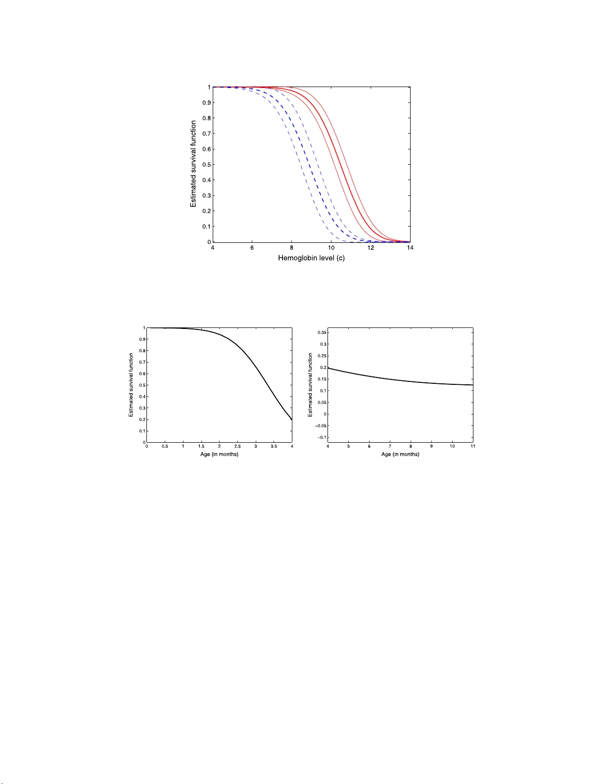
IMS Collectio ns Beyond P arametr ics in Interdisciplinary Resear c h: F estsc hrift in Honor of Professor Pranab K. Sen V ol. 1 (2008) 123– 137 c  Institute of Mathematical Stat istics , 2008 DOI: 10.1214/ 193940307 000000095 Estimation of p op ulation-le v e l summaries in general semiparametric rep eate d measures regress ion m o dels ∗ Arnab Mait y 1 , T atiy ana V. Apanaso vich 2 and Ra ym ond J. Carroll 1 T exas A&M Universit y , Cornel l Universit y and T exas A& M University Abstract: This paper considers a wide family of semiparametric repeated measures regression mo dels, in whic h the main interest is on e stimating population-level quan tities such as mean, v ariance, probabilities etc. Examples of our framework include generalized linear mo dels for clustered/longitud inal data, a mong man y others. W e d erive pl ug-in k ernel-based estimators of the population lev el quant ities and derive their asymptotic distri bution. An exam- ple in vo lving estimation of the surviv al function of hemoglobin measures i n the Ken ya hemoglobin study data is present ed to demonstrate our metho dology . 1. In tro duction This pap er is ab out s emiparametric r egressio n mo dels with rep eated mea s ures when the pr imary go al is to estimate a populatio n quantit y such a s mean, v ariance, pro b- ability , etc. W e will construct estimators of these quan tities which utilize the under - lying semiparametr ic s tructure of the mo del and der ive their limiting distribution. The work is motiv ated by the following example: the K eny a hemog lo bin data. The goal is to study the changes of hemoglobin over time during the firs t year of birth. The data s e t consists of 68 families with 2 children p er family . F or each child, 4 rep eated measures are taken over time in the first year since bir th: the time of visit v ar ied fro m c hild to child. The factors include mother’s age at child birth, child sex and placental paras itemia density (PDEN), a mar ker of malar ia that c ould affect hemoglobin. T o mo del these data, Lin and Carro ll [ 2 ] co nsidered a semiparametric mo del wher e the mother ’s a ge effect is mo deled no nparametrica lly and (sex, PDEN) is mo deled pa rametrically . The mo del is giv en b y the r ep eated measures par tially linear mo del Y ij k = X T ij k β 0 + θ 0 ( Z ij ) + ǫ ij k , (1.1) where i = 1 , . . . , n , j = 1 , . . . , m and k = 1 , . . . , R . Sp ecifically , Lin a nd Ca rroll [ 2 ] set Y ij k = hemog lobin level of the j th child in the i th family at the k th visit, Z ij = ∗ Supported b y gr ants from the National Cancer Institute (CA57030, C A 104620) and by the T exas A&M Center for Environmen tal and Rural Health via a gran t from the National Institute of En vironmen tal Health Sciences (P30-ES09106). 1 Departmen t of Stat istics, T exas A&M Univ ersity , College Station, TX 7784 3-3143, USA, e-mail: amaity@s tat.tamu. edu ; carroll@stat. tamu.edu 2 Sc hool of Op erations Researc h and Industrial Engineering Cornell U ni v ersity , Ithaca NY 14853, USA, e-mail: tva2@cor nell.edu AMS 2000 subje ct classific ati ons: Pr i mary 62G08, 62J02; secondary 62J12. Keywor ds and phr ases: clustered/longitudinal data, generalized estimating equations, gener- alized linear m i xed models, ke rnel metho d, marginal mo dels, measurement error, nonparametric regression, partiall y l inear mo del, profile metho d, repeated measures. 123 124 A. Maity T. V. Ap anasovich and R. J. Carr ol l mother’s a g e at the j th child birth in the i th family , X ij k = { sex, logp den, month, (mont h − 4) + } , where sex = 1 if female and 0 if male, logp den = log(PDEN+1), month denotes the age of the child at the k th visit a nd the function f + = f if f > 0 and 0 if f ≤ 0. As noted by Lin a nd Carro ll [ 2 ], the cov ar iates { mon th, (mont h − 4) + } ar e used to mo del the time effect as a piecewise linear function with a knot a t 4 months: this trend b eing observed by preliminar y ana ly sis of the data set. Also assume that, ǫ i = ( ǫ i 11 , ǫ i 12 , . . . , ǫ imR ) has a Nor mal(0 , Σ) distribution with Σ = σ 2 I mR + ρσ 2 ( J mR − I mR ), where I mR is the mR × mR identit y matrix and J mR is a mR × mR ma trix with 1 a s a ll elements. In this context, apa rt from the mo del comp onents, namely β 0 and θ 0 ( • ), one is interested in o ther p o pulation level quan tities suc h as mean hemoglo bin, E ( Y ) or v arious probabilities such as the propo rtion of six month o ld children who have hemoglobin measure a b ove a given constant c , pr ( Y > c | month = 6), etc. Note that each of the a b ov e-men tioned po pulation-level quantities can be written as functions of X , Z and the mo del parameters . F or example, b eca us e Z , sex and logp den a r e indep endent of mo nth, we can write pr( Y > c | month = a ) = E  Φ[ { X T β 0 + θ 0 ( Z ) − c } /σ ] | month = a  , (1.2) where c and a a r e given constant s and Φ( • ) is the standard nor ma l cdf. In general, we can consider any functional κ 0 = E {F ( • ) } for some function F ( • ): this o f co urse includes such quantities as p opulation mean, proba bilities, etc. The K eny a hemo globin study exa mple is a sp ecial cas e of a muc h mor e gener a l framework, one w e call semipara metric rep eated measures regres s ion modeling . Let e Z i = ( Z i 1 , . . . , Z im ) and let e Y i and e X i be the ensemble of resp o nses a nd other cov a riates, res pec tively . Consider a semipar ametric problem in which the loglike- liho o d function co nditional on ( e X , Z 1 , . . . , Z m ) is L{ e Y , e X , θ 0 ( Z 1 ) , . . . , θ 0 ( Z m ) , B 0 } , where B 0 is the set of model parameters. Also as an imp or tant g eneralizatio n, allow e Y to b e partially missing a nd let δ = 1 if e Y is o bserved and 0 o therwise. Supp ose further that e Y is missing at r andom, so that pr( δ = 1 | e Y , e X , e Z ) = pr( δ = 1 | e X , e Z ). If we de fine L B ( • ) and L j θ ( • ) to b e the deriv ativ es o f the loglikelihoo d with resp ect to B a nd θ ( Z j ), we hav e the pr op erties that for j = 1 , 2 , . . . , m , E [ δ L B { e Y , e X , θ 0 ( Z 1 ) , . . . , θ 0 ( Z m ) , B 0 }| e X , Z 1 . . . , Z m ] = 0; E [ δ L j θ { e Y , e X , θ 0 ( Z 1 ) , . . . , θ 0 ( Z m ) , B 0 }| e X , Z 1 . . . , Z m ] = 0 . The main g o al o f this pa pe r is to estimate a po pulation level qua nt ity , namely κ 0 = E [ F { e X , e Z , θ 0 ( Z 1 ) , . . . , θ 0 ( Z m ) , B 0 } ] (1.3) for an arbitr ary but s mo oth function F ( • ). F or example, in ( 1.2 ) we hav e F ( • ) = Φ[ { X T β 0 + θ 0 ( Z ) − c } /σ ] wher e last tw o c omp onents of X are fixed as a and ( a − 4) + . Although there are v arious papers ab out application of semiparametric methods in the context of long itudinal data (see for example Zeger and Diggle [ 5 ] and Zhang et a l. [ 6 ]), to the b est of our knowledge there is no liter ature on estimation of arbitrar y p opulation-level quantities in the r ep e ated-measures co nt ext. See Ma it y et al. [ 3 ] for the case of no rep eated measurement. How ever, estimation of B 0 and θ 0 ( • ) is describ ed in Lin and Carr oll [ 2 ]. If we call their estimates b B and b θ ( • , b B ), then we pro p o se to estimate the p opulation-level quantit y a s b κ semi = n − 1 n X i =1 F { e X i , e Z i , b θ ( Z i 1 , b B ) , . . . , b θ ( Z im , b B ) , b B } . (1.4) Semip ar ametric r ep e ate d me asur es r egr ession 125 In this pap er, we a r e int erested in the a symptotic b ehavior of b κ semi . This pap er is or ganized as follo ws. In Section 2 , we discuss the genera l semipara- metric problem with lo glikelihoo d L ( • ) and a gene r al goal of estimating κ 0 . W e also der ive the as y mptotic distribution of ( 1.4 ). In Section 3 , we demonstrate our metho d by applying it to analyz e the Kenya hemoglobin study data. All technical results are given in an Appe ndix . 2. Semiparametric mo de ls with multiple comp onents 2.1. Mo del c omp onent estimati on Estimation o f B 0 and θ 0 ( • ) using pr ofile likelihoo d and ba ckfittin g metho ds is dis- cussed in deta il in Lin and Ca r roll [ 2 ] when ther e are no missing data. With miss- ing data, the metho d works as follows. Let K ( • ) b e a smo o th symmetric density function with b ounded supp or t a nd v ar iance 1 . 0, let h b e a bandwidth and let K h ( z ) = h − 1 K ( z /h ). Define G ij ( z , h ) = { 1 , ( Z ij − z ) /h } . F or any fixed B = B ∗ , let b θ c ( • ) be the current estimate in an iter ative pro cedur e and ( b α 0 , b α 1 ) be the solution of the following estimating equation: 0 = n X i =1 m X j =1 δ i K h ( Z ij − z ) G ij ( z , h ) ×L j θ n e Y i , e X i , b θ c ( Z i 1 , B ∗ ) , . . . , α 0 + α 1 ( Z ij − z ) , . . . , b θ c ( Z im , B ∗ ) o . W e then up date b θ ( • ) as b θ ( z , B ∗ ) = b α 0 . T o estimate B 0 , a ba ckfitting algo rithm can b e used. In the itera ted backfitting algorithm, suppos e the current estimate is B ∗ . Then the backfittin g e s timator o f B 0 mo dified for missing resp onses is up dated by ma ximizing in B the function n X i =1 δ i L n e Y i , e X i , b θ ( Z i 1 , B ∗ ) , . . . , b θ ( Z im , B ∗ ) , B o , i.e., solving for B 0 = n X i =1 δ i L B n e Y i , e X i , b θ ( Z i 1 , B ∗ ) , . . . , b θ ( Z im , B ∗ ) , B o . The final estimates are o btained by iterating the pro cess until conv ergence. 2.2. Estimation of gener al p opulation-l evel summaries W e take a dv antage of the r e sults a bo ut the a symptotic expansions for b B a nd b θ ( • ) provided in Lin and Car roll [ 2 ], with the mo dification o f incor p o rating the missing data indicator s. Let L j kθ ( • ) = ∂ L j θ { Y , X , θ 0 ( Z 1 ) , . . . , θ 0 ( Z m ) , B 0 } /∂ θ ( Z k ). Make the definitions Ω( z ) = P m j =1 f j ( z ) E { δ L j j θ ( • ) | Z j = z } and A ( B , z 1 , z 2 ) = m X j =1 m X k 6 = j f j ( z 1 ) E { δ L j kθ ( • ) B ( Z k , z 2 ) / Ω( Z k ) | Z j = z 1 } ; Q ( z 1 , z 2 ) = m X j =1 m X k 6 = j f j k ( z 1 , z 2 ) E { δ L j kθ ( • ) | Z j = z 1 , Z k = z 2 } / Ω( z 2 ) , 126 A. Maity T. V. Ap anasovich and R. J. Carr ol l where f j ( z ) is the density o f Z j and f j k ( z 1 , z 2 ) is the biv ariate density of ( Z j , Z k ), assumed to ha ve bo unded supp or t and are p os itive o n the supp ort. Let G ( z 1 , z 2 ) be the solution to G ( z 1 , z 2 ) = Q ( z 1 , z 2 ) − A ( G , z 1 , z 2 ) . Define L j θ B ( • ) = ∂ L j θ { e Y , e X , θ 0 ( Z 1 ) , . . . , θ 0 ( Z m ) , B 0 } /∂ B and ǫ # ij ( θ, B ) = L j θ B { e Y i , e X i , θ ( Z i 1 ) , . . . , θ ( Z im ) , B } + m X k =1 L j kθ { e Y i , e X i , θ ( Z i 1 ) , . . . , θ ( Z im ) , B } θ B ( Z ik , B ) , (2.1) where θ B ( z , B 0 ) satisfies 0 = m X j =1 f j ( z ) E { δ ǫ # ij ( θ 0 , B 0 ) | Z j = z } . (2.2) Define ǫ i = L i B ( • ) + m X j =1 L ij θ ( • ) θ B ( Z ij , B 0 ); M 1 = E ( δ ǫǫ T ) = − E { δ i L BB ( • ) + m X j =1 δ i L j θ B ( • ) θ T B ( Z j , B 0 ) } . Define the der iv atives of F ( • ) in a similar wa y to L ( • ) and make the following definitions: M 2 = E [ F B ( • ) + m X j =1 F j θ ( • ) θ B ( Z j , B 0 )]; C 1 ( z ) = − m X j =1 f j ( z ) E { F j θ ( • ) | Z j = z } / Ω( z ); C 2 ( z ) = E [ m X j =1 E {F j θ ( • ) | Z j }G ( Z j , z ) / Ω( Z j )]; D ( • ) = m X j =1 L j θ ( • ) { C 1 ( Z j ) + C 2 ( Z j ) } . Then we hav e the following result. Theorem 2.1. Assume that ( e Y i , δ i , e X i , Z i 1 , . . . , Z im ) , i = 1 , 2 , . . . , n ar e indep en- dently and identic al ly distribute d and nh 4 → 0 . Then, t o terms of or der o p (1) , n 1 / 2 ( b κ semi − κ 0 ) ≈ n − 1 / 2 n X i =1 {F i ( • ) − κ 0 + M T 2 M − 1 1 δ i ǫ i + δ i D i ( • ) } (2.3) → Normal (0 , V κ ) , (2.4) wher e V κ = E {F ( • ) − κ 0 } 2 + M T 2 M − 1 1 M 2 + E { δ D 2 ( • ) } . Semip ar ametric r ep e ate d me asur es r egr ession 127 Note that w e have ass umed that κ 0 = E [ F { e X , e Z , θ 0 ( Z 1 ) , . . . , θ 0 ( Z m ) , B 0 } ] a nd F ( • ) a re scalar, whic h in principle excludes the estimation of quantities suc h as the po pula tion v ariance and standard deviation. How ever, the result can be re a dily generalized to handle this case . In gener al, supp os e κ 1 = E {F 1 ( • ) } and κ 2 = E {F 2 ( • ) } for some smo oth functions F 1 ( • ) and F 2 ( • ), and are estimated by b κ 1 and b κ 2 , resp ectively . Supp ose that we are in terested in κ gen = g ( κ 1 , κ 2 ) for some function g ( • , • ). Then we have the following res ult: Corollary 2.1. L et κ gen b e estimate d by b κ gen = g ( b κ 1 , b κ 2 ) and that g ( • , • ) is dif- fer entiable with r esp e ct to b oth of its ar guments. L et g 1 ( • , • ) and g 2 ( • , • ) b e the derivatives of g with re sp e ct to its first and se c ond ar gument, r esp e ct ively. Then we have n 1 / 2 ( b κ gen − κ gen ) = n 1 / 2 g 1 ( κ 1 , κ 2 )( b κ 1 − κ 1 ) + n 1 / 2 g 2 ( κ 1 , κ 2 )( b κ 2 − κ 2 ) + o p (1) → Normal (0 , V gen ) , with V gen = g 2 1 ( κ 1 , κ 2 ) V 1 + g 2 2 ( κ 1 , κ 2 ) V 2 + 2 g 1 ( κ 1 , κ 2 ) g 2 ( κ 1 , κ 2 ) V 12 , wher e V 1 and V 2 ar e asymptotic vari anc es of b κ 1 and b κ 2 , r esp e ctively, c ompute d using ( 2.4 ) and V 12 = E [ {F 1 ( • ) − κ 1 }{F 2 ( • ) − κ 2 } ] . Remark 2.1. W e note that if κ 0 were a function of only B 0 , then a bandwidth prop ortiona l to h ∼ n − 1 / 5 can b e used, b ecause in this case under smo othing is no t necessary . The rea son for the under smo othing in the g eneral ca se is the inclusion of θ 0 ( • ) in κ 0 . Using the res ults fro m Lin and Carro ll [ 2 ] we hav e b θ ( z ) − θ 0 ( z ) = O p ( h 2 ) − n − 1 n X i =1 m X j =1 δ i K h ( Z ij − z ) L ij θ ( • ) / Ω( z ) + n − 1 n X i =1 m X j =1 δ i L ij θ ( • ) G ( z , Z ij ) / Ω( z ) + o p ( n − 1 / 2 ) . The restriction nh 4 → 0 re mov es the O p ( h 2 ) bias term. It is sugge s ted in Sepa- nski et a l. [ 4 ] that in man y semiparametric pr oblems, the optimal bandwidth for estimating parameters s uch as B 0 is o f the order n − 1 / 3 , which of course satisfies nh 4 → 0. In the case of no rep eated measures, i.e., when m = 1, Maity et a l. [ 3 ] find that they hav e goo d exper ience numerically by first estimating the bandwidth via lik eliho o d cros s v alidation, which will be o f order n − 1 / 5 , and then m ultiplying it by n − 2 / 15 to get the bandwidth to b e of order n − 1 / 3 . Remark 2.2. T o estimate the asymptotic v a riance o f κ 0 , o ne can use the b o otstr ap metho d. While the justification of use of par a metric bo otstrap for estimatio n of mo del parameter s is pr ovided in C he n et al. [ 1 ], we conjecture that the bo o tstrap works for κ 0 as well. O ne ca n also use the plug-in metho d where one r eplaces each term in the v ariance expressio n in ( 2.4 ) b y their consistent estimators . Constructing consistent estimators fo r the firs t tw o terms are fairly stra ightforw ard wher e one merely replaces all the exp ectations by sums in that expr ession and all the r egress io n functions by k ernel estimates. How ever, the main difficult y lies in the estimatio n of the third term where one has to solve the functional equatio n G ( z 1 , z 2 ) = Q ( z 1 , z 2 ) − A ( G , z 1 , z 2 ) for G ( • , • ), which can b e numerically difficult. 2.3. Gener al functions of the r esp onse One interesting and imp orta nt sce nario is when κ 0 can b e c o nstructed using only the resp onses. Suppose that κ 0 = E {G ( e Y ) } . Also define F { e X , e Z , θ 0 ( Z 1 ) , . . . , θ 0 ( Z m ) , 128 A. Maity T. V. Ap anasovich and R. J. Carr ol l B 0 } = E {G ( e Y ) | e X , e Z } . In the presence of miss ing data, there are v arious e stimators one can use. W e will dis cuss t w o of these e s timators whic h are ba sed upon different constructions for es tima ting the missing data pro ces s. Let b F i ( • ) = F { e X i , e Z i , b θ ( Z i 1 , b B ) , . . . , b θ ( Z im , b B ) , b B } . T o form the first estimator, we impute G ( e Y i ) by b F i ( • ) for every missing e Y i . W e estimate κ 0 by b κ 1 = n − 1 n X i =1 { δ i G ( e Y i ) + (1 − δ i ) b F i ( • ) } . Note that in absence of missing data, b κ 1 do es not use the semiparametric mo del and is co nsistent. If the resp onses are mis s ing a t ra ndom, then b κ 1 is consistent if the semipara metric mo del s pe c ification is cor rect. The sec o nd estimator depends o n the underlying str uc tur e o f the miss ing data pro cess where we assume a parametric for mulation for estimating pr( δ = 1 | e Y , e X , e Z ) = π ( e X , e Z , ζ ), where ζ is an unknown para meter estimated by standard logis tic regres s ion of δ on ( e X , e Z ). Then co nstruct the estimator b κ 2 = n − 1 n X i =1  δ i π ( e X i , e Z i , b ζ ) G ( e Y i ) +  1 − δ i π ( e X i , e Z i , b ζ )  b F i ( • )  . This e s timator has the double- robustness pro pe rty that if either the semiparametric mo del sp ecification for ( θ 0 , B 0 ) or the para metric mo del for π ( e X , e Z , ζ ) is correct, b κ 2 is consistent and has a n a symptotic nor mal distribution. If both the mo dels are corr ect then the following results are true. The pro ofs are given in the App endix. Lemma 2.1. Define M 2 , imp = E [(1 − δ ) { F B ( • ) + m X j =1 F j θ ( • ) θ B ( Z j , B 0 ) } ]; C 1 , imp ( z ) = − m X j =1 f j ( z ) E { (1 − δ ) F j θ ( • ) | Z j = z } / Ω( z ); C 2 , imp ( z ) = E [ m X j =1 E { (1 − δ ) F j θ ( • ) | Z j }G ( Z j , z ) / Ω( Z j )]; D imp ( • ) = m X j =1 L j θ ( • ) { C 1 , imp ( Z j ) + C 2 , imp ( Z j ) } . Assume that nh 4 → 0 . Then, t o terms of or der o p ( n − 1 / 2 ) , b κ 1 − κ 0 ≈ n − 1 n X i =1 n δ i G ( e Y i ) + (1 − δ i ) F i ( • ) − κ 0 + M T 2 , imp M − 1 1 δ i ǫ i + δ i D i, imp ( • ) o . (2.5) Lemma 2.2. Define π ζ ( e X , e Z , ζ ) = ∂ π ( e X , e Z , ζ ) /∂ ζ . Assu me that n 1 / 2 ( b ζ − ζ ) = n − 1 / 2 P n i =1 ψ iζ ( • ) + o p ( n − 1 / 2 ) with E { ψ ζ ( • ) | e X , e Z } = 0 . A lso assu me that nh 4 → 0 . Semip ar ametric r ep e ate d me asur es r egr ession 129 Then, to terms of or der o p ( n − 1 / 2 ) , b κ 2 − κ 0 ≈ n − 1 n X i =1  δ i π ( e X i , e Z i , ζ ) {G ( e Y i ) − κ 0 } +  1 − δ i π ( e X i , e Z i , ζ )  {F i ( • ) − κ 0 }  . (2.6) Remark 2.3. The expansions ( 2 .5 ) and ( 2.6 ) show that b κ 1 and b κ 2 are asymptot- ically nor mally distributed. One can show that the asymptotic v ar iances a re given as V κ 1 = v ar  δ G ( e Y ) + (1 − δ ) F ( • ) + M T 2 , imp M − 1 1 δ ǫ + δ D imp ( • )  ; V κ 2 = v ar  δ π ( e X , e Z , ζ ) G ( e Y ) +  1 − δ π ( e X , e Z , ζ )  F ( • )  , resp ectively , from which e s timates a re readily der ived. Note tha t the estimation of B 0 and θ 0 ( • ) has no impact on the a symptotic distribution of b κ 2 . Hence it has the distinct adv an tage that its limiting distribution do es not inv olve an integral equation. 3. Application 3.1. Motivating example W e applied our metho d to analyze the K eny a hemoglo bin data which is describ ed in Section 1 . The mo del is given by ( 1.1 ) where n = 68, m = 2 and R = 4. Comparing this to the gener al mo del, we s ee that e Y i = ( y i 11 , . . . , y i 24 ) T , e X i = ( X i 11 , . . . , X i 24 ) T and Z i 1 = Z i 2 = Z i 3 = Z i 4 and Z i 5 = Z i 6 = Z i 7 = Z i 8 . Also, B = ( β T , σ ) T . Let e 4 be a vector of ones of length 4. The loglikelihoo d function, conditional of e X a nd ( Z 1 , Z 2 ), is that of a multiv a riate Gaussian distribution with mean e X T β 0 + { θ 0 ( Z 1 ) e T 4 , θ 0 ( Z 2 ) e T 4 } T and cov ariance ma trix Σ. Recall that we a re in terested in the prop or tion of all children of a given ag e a who hav e their hemo g lobin measure above any given constant c , which is defined as κ 0 = E  Φ[ { X T β 0 + θ 0 ( Z ) − c } /σ ] | month = a  . (3.1) Note tha t the joint density of ( Z , sex , lo g p den) is indep endent of “month” and hence the conditional exp ectation in ( 3.1 ) can be wr itten as E (Φ[ { X T β 0 + θ 0 ( Z ) − c } /σ ]) with the last tw o comp onents o f X being fixed as a and ( a − 4) + . Using this fact, we estimate κ 0 by b κ semi = { nmR } − 1 n X i =1 m X j =1 R X k =1 Φ[ { X T ij k b β + b θ ( Z ij , b β ) − c } / b σ ] , (3.2) where the last tw o comp onents of X ij k are fix ed as a a nd ( a − 4) + . Also no te tha t there ar e no mis s ing resp onses inv olv ed in this setup. W e pr o ceed to es tima te B 0 and θ 0 ( • ) as indicated in Lin and Carro ll [ 2 ] and use these es tima tes to compute ( 3.2 ). W e e s timate b κ semi for a = 3 , 6 a nd for different 130 A. Maity T. V. Ap anasovich and R. J. Carr ol l Fig 1 . R esults for t he Ke ny a hemo globin data example. Plotte d ar e est imate d survival function (1 − the c df ) of hemo globin me asur e of childr en of a give n age a , along with 95% c onfidenc e intervals. Dashe d lines c orr esp ond to six-month-old c hildr en and solid lines c orr esp ond to thr e e- month-old childr en. Fig 2 . R esults for t he Ke ny a hemo globin data example. Plotte d ar e est imate d survival function (1 − the c df ) for a fixe d hemo globin level c = 10 as age varies fr om 0.1 months to 4 months (left p anel) and 4 months t o 11 months (right p anel). v alues of c . W e estimate the limiting v ariances via the bo o tstrap and use those to constr uct 95% co nfidence interv als. The results ar e display ed in Figure 1 . It is interesting to note that the t w o estimates differ significa nt ly a nd a decrease in prop ortion is evident a s the age o f the children increases . W e can o bserve form Figure 1 that for a given hemoglo bin level, the pro po rtion of children having a higher hemo globin level at a ge three is significantly less than at age s ix , indicating an increase in r is k of getting a ne mia (low hemoglobin level) a s children g row older . T o obs e rve this effect, we set the hemog lo bin le vel, c = 10 a nd estimated the surviv al function ov er a g r id of v alue for age, a . Since the time effect is mo de le d as a piecewise linear function with a knot at 4 months, w e plot the estimated surviv a l function in t wo different plo ts in Figure 2 : left panel displays the surviv al function a s age v aries in [0 . 1 , 4] and right panel plots the surviv al function when age v aries in (4 , 11]. The decrease in hemoglo bin level is muc h faster for children b elow age 4 months than children older than 4 mo nt hs, after which the sur viv al function b eco mes flatter. Semip ar ametric r ep e ate d me asur es r egr ession 131 Note that one c a n construct other estimato rs for κ 0 , for example, the s ample av erage of hemoglobin mea sures of o nly those children w ho hav e a ge a . How ever, it is impo rtant to note that the naive estima to r do es not use the informa tion that “month” is indep e ndent of ( Z , sex , logp den). On the o ther hand, this vital informa- tion is use d to cons tr uct the semipar ametric estimator thus allowing b κ to b e more efficient than the naiv e estimator . Also , note that in this example the use of the usual naive estimators may not b e justified b ecaus e the nu mber of children of any given age a may b e very small. In fact, ther e a re only six children with age a = 3 and o nly one child with age a = 6 in the data set we used. This pro blem do es no t arise when b κ semi is used b ecause of the fact that it us es all the da ta to estimate κ 0 rather than using o nly those children who have age a . 3.2. Simulation study W e co nducted a small simulation study to obs e rve the p erforma nce o f our metho d. W e considered the mo de l given in ( 1.1 ) with n = 1 00 clus ter s with s ix mea surements per cluster. Sp ecifica lly , w e set m = 2 and R = 3 with Z i 1 = Z i 2 = Z i 3 and Z i 4 = Z i 5 = Z i 6 . W e assume that ǫ i has a Nor mal(0 , Σ) distr ibutio n with Σ = σ 2 I mR + ρσ 2 ( J mR − I mR ). W e set σ 2 = 1 and ρ = 0 . 4 . W e gener ated Z from a uniform(0 , 1) distribution with the true function θ 0 ( z ) = sin(8 z − 1). The individual comp onents of X are g enerated from uniform(0 , 1 ) distribution, indep endent of each other and Z . The true v alue of β 0 = [1 , 1] T . In this setup, o ur tar get was to estimate κ 0 ( c ) = pr( Y > c | X 1 = 0 . 5 ) = E  Φ[ { X T β 0 + θ 0 ( Z ) − c } /σ ] | X 1 = 0 . 5  for a given v a lue of c , wher e X 1 denotes the first compo nent of X . W e estimate κ 0 ( c ) by b κ ( c ) = { nmR } − 1 n X i =1 m X j =1 R X k =1 Φ[ { X T ij k b β + b θ ( Z ij , b β ) − c } / b σ ] , where the first comp onent of X ij k is fix e d to be 0 . 5. Note a gain that in definitio n of b κ ( c ), we used indep endence b etw een X and Z to our adv a nt age. W e employ ed the metho d in Lin and Car roll [ 2 ] with the Epanechnik ov kernel function to o btain b β a nd b θ ( • ). Using thes e estimates we calculated b κ ( c ) ov er a grid of v alues for c . Also the true surviv a l function was computed analytica lly . W e generated 1000 data sets, with r esults displayed in Figure 3 . It is evident that the estimated surv iv al function g iven by our metho d is very close to the true function, as one w ould exp ect for large sample size. Note that X is g enerated from a con tin uous distribution and hence the use of naive es timator is not justified in this case. 4. Discussion In this pape r, we considered a genera l class of semipara metric mo dels, with re- sp onses missing at ra ndom, where the prima ry go al w as to estimate p opulation- level quant ities κ 0 such as the mean, probabilities, etc. F or general se miparametric regres s ion mo dels , the a s ymptotic distribution of a plug-in estimator of κ 0 was derived. 132 A. Maity T. V. Ap anasovich and R. J. Carr ol l Fig 3 . R esults for the simulation study b ase d on 1000 simulate d data set s. Plotte d ar e the true survival function (dashe d line), the me an estimate d survival funct ion (1 − the c df ) (solid line), along with a 95% c onfidenc e r ange(dash-dotte d line). W e hav e co nsidered the case that the unknown function θ 0 ( Z ) was a scalar function of a scalar argument. The results tho ugh r eadily extend to the case of a m ultiv aria te function of a scala r a r gument. App endix A: Sk etc h of technical argumen ts A.1. Sketch of The or em 2.1 W e first show ( 2.3 ). Firs t note that L is a loglikelihoo d function conditioned on ( X, Z ), so tha t we hav e E { δ L j kθ ( • ) | e X , e Z } = − E { δ L j θ ( • ) L kθ ( • ) | e X , e Z } ; E { δ L j θ B ( • ) | e X , e Z } = − E { δ L j θ ( • ) L B ( • ) | e X , e Z } . (A.1) Also, it follows fro m Lin and Carroll [ 2 ], and h = o p ( n − 1 / 4 ) that b θ ( z , B 0 ) − θ 0 ( z ) = − n − 1 n X i =1 m X j =1 δ i K h ( Z ij − z ) L ij θ ( • ) / Ω( z ) + n − 1 n X i =1 m X j =1 δ i L ij θ ( • ) G ( z , Z ij ) / Ω( z ) + o p ( n − 1 / 2 ); (A.2) b B − B 0 = M − 1 1 n − 1 n X i =1 δ i ǫ i + o p ( n − 1 / 2 ) . (A.3) Semip ar ametric r ep e ate d me asur es r egr ession 133 By a T aylor e xpansion, n 1 / 2 ( b κ − κ 0 ) = n − 1 / 2 n X i =1  F i ( • ) − κ 0 + {F i B ( • ) + m X j =1 F ij θ ( • ) θ B ( Z ij , B 0 ) } T ( b B − B 0 ) + m X j =1 F ij θ ( • ) { b θ ( Z ij , B 0 ) − θ 0 ( Z ij ) }  + o p (1) = n − 1 / 2 n X i =1 {F i ( • ) − κ 0 } + M T 2 n 1 / 2 ( b B − B 0 ) + n − 1 / 2 n X i =1 m X j =1 F ij θ ( • ) { b θ ( Z ij , B 0 ) − θ 0 ( Z ij ) } + o p (1) . Because nh 4 → 0 , using ( A.2 ), we see n − 1 / 2 n X i =1 m X j =1 F ij θ ( • ) { b θ ( Z ij , B 0 ) − θ 0 ( Z ij ) } = − n − 1 / 2 n X i =1 m X j =1 F ij θ ( • )[ n − 1 n X k =1 m X ℓ =1 δ k K h ( Z kℓ − Z ij ) L kℓθ ( • ) / Ω( Z ij )] + n − 1 / 2 n X i =1 m X j =1 F ij θ ( • )[ n − 1 n X k =1 m X ℓ =1 δ k L kℓθ ( • ) G ( Z ij , Z kℓ ) / Ω( Z ij )] + o p (1) = n − 1 / 2 n X k =1 m X ℓ =1 δ k L kℓθ ( • ) C 1 ( Z kℓ ) + n − 1 / 2 n X k =1 m X ℓ =1 δ k L kℓθ ( • ) C 2 ( Z kℓ ) + o p (1) = n − 1 / 2 n X i =1 δ i D i ( • ) + o p (1) . Result ( 2.3 ) now follows fro m ( A.3 ). Next, we show ( 2.4 ). Recall that, ǫ = L B ( • ) + P m j =1 L j θ ( • ) θ B ( Z j , B 0 ) and D ( • ) = P m j =1 L j θ ( • ) { C 1 ( Z j ) + C 2 ( Z j ) } . W e use ( 2.1 ), ( 2.2 ) and ( A.1 ) to derive that E { δ ǫD ( • ) } = − m X j =1 E  δ L j θ B ( • ) + m X k =1 δ L j kθ ( • ) θ B ( Z k , B 0 )  × { C 1 ( Z j ) + C 2 ( Z j ) }  = − E  m X j =1 E { δ ǫ # j ( θ 0 , B 0 ) | Z j }{ C 1 ( Z j ) + C 2 ( Z j ) }  = 0 . Also using the facts that E { D ( • ) | e X , e Z } = 0 and E ( ǫ | e X , e Z ) = 0, it is rea dily s e en 134 A. Maity T. V. Ap anasovich and R. J. Carr ol l that E [ {F ( • ) − κ 0 } D ( • )] = 0; E [ {F ( • ) − κ 0 } ǫ ] = 0 , which in tur n pr ove that all three terms in ( 2.3 ) are unco rrelated. Then ( 2.4 ) follows easily from the central limit theorem. A.2. Sketch of Cor ol lary 2.1 By a T aylor’s series expansio n, b κ gen − κ gen = { g 1 ( κ 1 , κ 2 )( b κ 1 − κ 1 ) + g 2 ( κ 1 , κ 2 )( b κ 2 − κ 2 ) } + o p ( n − 1 / 2 ) . Then, the nor mality follows from central limit theo rem. The v a riance calculation is str aight for ward since ( 2.3 ) together with the fact E ( D | X , Z ) = E ( ǫ | X , Z ) = 0 implies that nE { ( b κ 1 − κ 1 )( b κ 2 − κ 2 ) } = E [ {F 1 ( • ) − κ 1 }{F 2 ( • ) − κ 2 } ] . A.3. Sketch of L emma 2.1 W e have that b κ 1 = n − 1 n X i =1 { δ i G ( e Y i ) + (1 − δ i ) b F i ( • ) } = A 1 + A 2 , say . B y a T aylor s e r ies expansion, A 2 = n − 1 n X i =1 (1 − δ i ) b F i ( • ) = n − 1 n X i =1 (1 − δ i )[ F i ( • ) + {F i B ( • ) + m X j =1 F ij θ ( • ) θ B ( Z ij , B 0 ) } T ( b B − B 0 ) + m X j =1 F ij θ ( • ) { b θ ( Z ij , B 0 ) − θ 0 ( Z ij ) } ] + o p (1) = n − 1 n X i =1 (1 − δ i ) F i ( • ) + M T 2 , imp ( b B − B 0 ) + n − 1 n X i =1 m X j =1 (1 − δ i ) F ij θ ( • ) { b θ ( Z ij , B 0 ) − θ 0 ( Z ij ) } + o p (1) . Semip ar ametric r ep e ate d me asur es r egr ession 135 Using ( A.2 ) and nh 4 → 0, we see n − 1 n X i =1 m X j =1 (1 − δ i ) F ij θ ( • ) { b θ ( Z ij , B 0 ) − θ 0 ( Z ij ) } = − n − 2 n X i =1 m X j =1 (1 − δ i ) F ij θ ( • ) n X k =1 m X ℓ =1 δ k K h ( Z kℓ − Z ij ) L kℓθ ( • ) / Ω( Z ij ) + n − 2 n X i =1 m X j =1 (1 − δ i ) F ij θ ( • ) n X k =1 m X ℓ =1 δ k L kℓθ ( • ) G ( Z ij , Z kℓ ) / Ω( Z ij ) + o p ( n − 1 / 2 ) = n − 1 n X k =1 m X ℓ =1 δ k L kℓθ ( • ) C 1 , imp ( Z kℓ ) + n − 1 n X k =1 m X ℓ =1 δ k L kℓθ ( • ) C 2 , imp ( Z kℓ ) + o p ( n − 1 / 2 ) = n − 1 n X i =1 δ i D i, imp ( • ) + o p ( n − 1 / 2 ) . The result now follows directly from ( A.3 ). A.4. Sketch of L emma 2.2 W e have that b κ 2 = n − 1 n X i =1  δ i π ( e X i , e Z i , b ζ ) G ( e Y i ) +  1 − δ i π ( e X i , e Z i , b ζ )  b F i ( • )  = A 1 + A 2 , say . B y a T aylor s e r ies expansion, A 1 = n − 1 n X i =1 δ i G ( e Y i ) π ( e X i , e Z i , ζ ) − E  G ( Y ) π ( e X , e Z , ζ ) π ζ ( e X , e Z , ζ )  T n − 1 n X i =1 ψ iζ + o p ( n − 1 / 2 ) . In addition, A 2 = B 1 + B 2 + o p ( n − 1 / 2 ); B 1 = n − 1 n X i =1  1 − δ i π ( e X i , e Z i , ζ )  b F i ( • ); B 2 = n − 1 n X i =1 δ i b F i ( • ) { π ( e X i , e Z i , ζ ) } 2 π ζ ( e X i , e Z i , ζ ) T ( b ζ − ζ ) + o p ( n − 1 / 2 ) . 136 A. Maity T. V. Ap anasovich and R. J. Carr ol l It follows eas ily that B 1 = n − 1 n X i =1  1 − δ i π ( e X i , e Z i , ζ )  F i ( • ) + n − 1 n X i =1 m X j =1  1 − δ i π ( e X i , e Z i , ζ )  F ij θ ( • ) { b θ ( Z ij , B 0 ) − θ 0 ( Z ij ) } + n − 1 n X i =1  1 − δ i π ( e X i , e Z i , ζ )  F T i B ( • )( b B − B 0 ) + n − 1 n X i =1  1 − δ i π ( e X i , e Z i , ζ )  m X j =1 F ij θ ( • ) θ T B ( Z i , B 0 )( b B − B 0 ) + o p ( n − 1 / 2 ) . Using 0 = E { 1 − δ π ( e X , e Z ,ζ ) | e X , e Z } a nd b B − B 0 = O p ( n − 1 / 2 ), we see that the thir d and fourth terms are o p ( n − 1 / 2 ). Also, using nh 4 → 0 and ( A.2 ) we see n − 1 n X i =1 m X j =1  1 − δ i π ( e X i , e Z i , ζ )  F ij θ ( • ) { b θ ( Z ij , B 0 ) − θ 0 ( Z ij ) } = − n − 1 n X i =1 m X j =1  1 − δ i π ( e X i , e Z i , ζ )  F ij θ ( • ) ×  n − 1 n X k =1 m X ℓ =1 δ k K h ( Z kℓ − Z ij ) L kℓθ ( • ) / Ω( Z ij )  − n − 1 n X i =1 m X j =1  1 − δ i π ( e X i , e Z i , ζ )  F ij θ ( • ) ×  n − 1 n X k =1 m X ℓ =1 δ k L kℓθ ( • ) G ( Z ij , Z kℓ ) / Ω( Z ij )  + o p ( n − 1 / 2 ) = o p ( n − 1 / 2 ) . The last step follows b ecause E [ { 1 − δ π ( e X , e Z ,ζ ) }F j θ ( • ) | e Z ] = 0 . Hence we s ee that B 1 = n − 1 n X i =1  1 − δ i π ( e X i , e Z i , ζ )  F i ( • ) + o p ( n − 1 / 2 ) . Similarly , using b ζ − ζ = O p ( n − 1 / 2 ), b B − B 0 = O p ( n − 1 / 2 ) and b θ ( z , B 0 ) − θ 0 ( z ) = O p ( n − 1 / 2 ), it also follows that B 2 = E  1 π ( e X , e Z , ζ ) F ( • ) π ζ ( e X , e Z , ζ )  T n − 1 n X i =1 ψ iζ ( • ) + o p ( n − 1 / 2 ) . The result now follows by collecting the terms. Ac knowledgmen ts. The authors thank Xihong Lin fo r providing the data used in this pap er. Semip ar ametric r ep e ate d me asur es r egr ession 137 References [1] Chen, X., Linton, O. and V an Keilegom, I. (200 3 ). E stimation of semi- parametric models when the c riterion function is not smoo th. Ec onometric a 71 1591 – 1608 . MR20002 59 [2] Lin, X. and Carroll, R. J. (2 006). Semipa r ametric estimation in general rep eated mea sures problems. J. R. Stat. So c. S er. B St at. Metho dol. 68 69–88. MR22125 75 [3] Maity, A., Ma, Y. and Carr oll, R. J. (20 07). Efficient estimation of p opulation- le vel summaries in general semipa rametric regr e ssion mo dels. J. Amer. Statist. Asso c. 1 02 123–1 39. MR22933 05 [4] Sep an ski, J. H ., Knickerbocker, R. and Carroll, R. J. (1994). A semi- parametric corr ection for a tten uation. J. Amer. St atist. As s o c. 89 13 66–1 373. MR13102 27 [5] Zeger, S. and Diggle, P. (19 94). Semipara metric mo dels for longitudinal data with application to c d4 cell num ber s in hiv sero co nv e r ters. Biometrics 50 689–6 99. [6] Zhang, D., Lin, X., Raz, J. and Sowers, M. (199 8). Semiparametric sto chastic mixed models for longitudinal data. J. A mer. S t atist. A sso c. 93 710–7 19. MR16313 69