In-season prediction of batting averages: A field test of empirical Bayes and Bayes methodologies

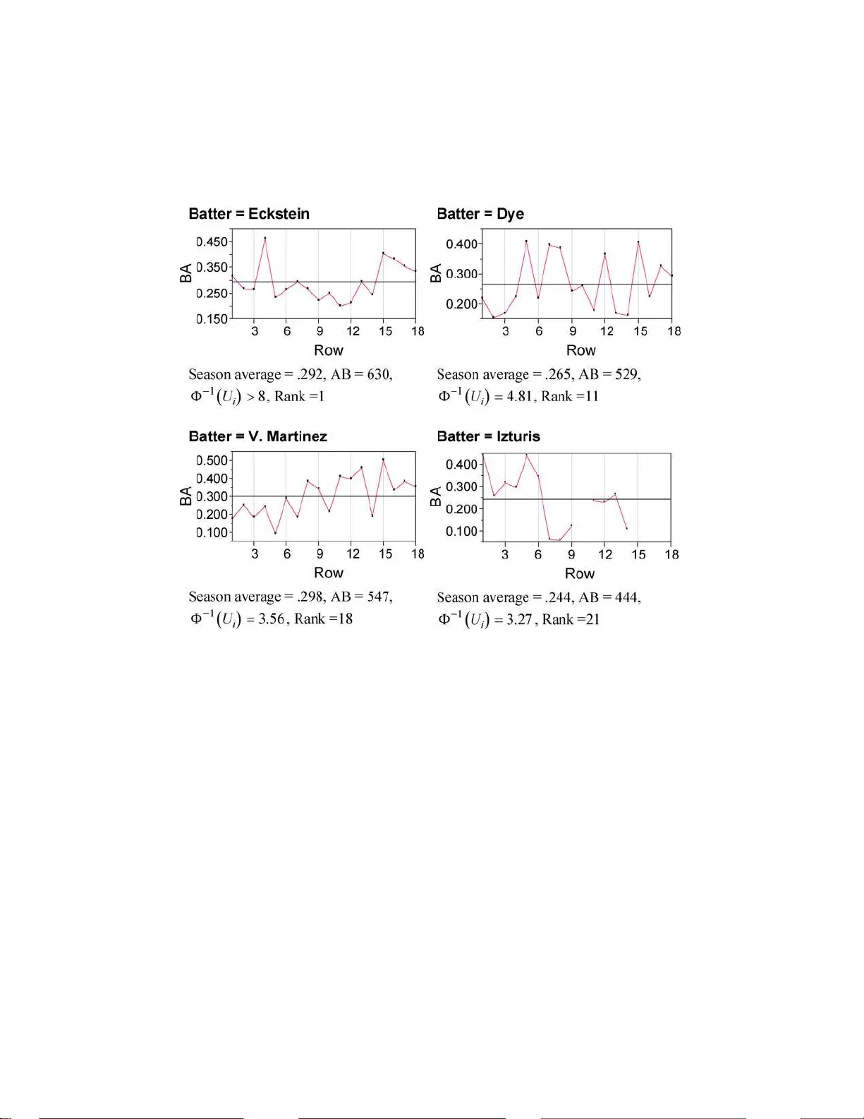
The Annals of Applie d Statistics 2008, V ol. 2, No. 1, 113–152 DOI: 10.1214 /07-A OAS138 c  Institute of Mathematical Statistics , 2 008 IN-SEASON PREDICTION OF BA TTING A VERAG ES: A FIELD TEST OF EMPIRICAL BA YES AND BA YES METHODOLOGIES 1 By La wrence D. Bro wn University of Pennsylvania Batting a vera ge is one of the principle p erformance measures for an individual baseball play er. It is natural to statistically mod e l this as a binomial-v ariable proportion, with a given (observed) num b er of q ual ifying attempts ( ca lled “at-bats”), an observ ed num b er of suc- cesses (“hits”) distributed according to the binomial distribution, and with a true (but unk no wn) v alue of p i that represents the pla yer’s laten t ability . This is a common d a ta structu re in many statistical applications; and so the meth odological study here h a s implications for such a range of applications. W e lo ok at batting records for each Ma jor League play er ov er the course of a single season (2005). The primary fo cus is on using only the batting records from an earlier part of th e season (e.g., the ﬁrst 3 months) in order to estimate the batter’s laten t ability , p i , and con- sequently , also to pred i ct their batting-a verage performance for the remainder of the season. Since we are using a season that has already concluded, we can then v alidate our estimation p erformance by com- paring th e estimated v alues to the actual v alues for the remainder of the season. The prediction metho ds to b e inve stigated are motiv ated from empirical Bay es and hierarchica l Ba yes interpretations. A n ewly pro- p osed nonparametric empirical Ba yes pro cedure p erforms p articu- larly w ell in the basic analysis of the full data set, t hough less well with analyses in vol ving more homogeneous sub sets of the data. In those more homogeneous situations b etter p erformance is obtained from appropriate versions of more familiar metho ds. In all situations the p o orest p erforming choice is the na ¨ ıve predictor which directly uses the current av erage to predict the futu re av erage. One feature of all the statistical metho dologies here is the prelimi- nary use of a new form of va riance stabilizing transformation in order to transform the binomial data problem into a somew hat more fa- miliar structure invo lving (approximately) N ormal rand om va riables Received Sep tember 2007; revised September 2007. 1 Supp orted in part by NSF Grant DMS-07-07033. Key wor ds and phr ases. Empirical Baye s, h ierarc hical Bay es, harmonic p rior, va riance stabilization, FD R, sp orts, hitting streaks, hot-hand. This is an ele c tronic reprint of the orig inal a rticle published by the Institute of Ma thematical Statistics in The Annals of Applie d Statistics , 2008, V ol. 2, No. 1, 11 3–15 2 . This reprint diﬀers from the or iginal in pagina tion and typogra phic detail. 1 2 L. D. BRO WN with known v ariances. This transformation technique is also used in the construction of a new empirical v alidation test of the binomial mod el assumption t hat is the conceptual basis for all our analyses. 1. In tro du ction. Overview. Batting av erage is one o f the principle p erformance measures for an individu al baseball pla y er. It is the p ercen tage of successful attempts, “Hits,” as a p rop ortion of the total n u m b er of qu alifying attempts, “At - Bats.” In sym b ols, the b atting a v erage of the i th play er ma y b e written as BA i = H i / AB i . This situation, with Hits as a n u mb er of successes within a qualifying n um b er o f attempts, mak es it natural to s tatistica lly mo del eac h pla yer’s batting a v erage as a binomial v ariable outcome, w ith a give n v alue of AB i and a tru e (but u nkno wn) v alue of p i that r epresen ts the pla y er’s laten t abilit y . As one outcome of our analysis we will demonstrate th at this m o del is a useful and reasonably accurate representati on of the s itu ation for Ma jor League pla yers o v er p erio d s of a month or longer within a giv en baseball season. (The season is appro ximately 6 mon ths long.) W e will look at batting records [Bro wn ( 2008 )] for eac h Ma jor League pla yer o v er the course of a single season (200 5). W e use the b atting r ecords from an earlier p art of the season (e.g., the ﬁrs t 3 months) in order to estimate the batter’s laten t ab ility , p i , and consequen tly , to predict their BA p erforman ce for th e remainder of th e season. Since we are using a season that has already concluded , w e can then v alidate the p erformance of our estimator by comparing the predicted v alues to the actual v alues for th e remainder of the season. Dual fo cus. Ou r study has a dual fo cus. One fo cus is to dev elop impro ved to ols for these predictions, along with relativ e measures of the attainable accuracy . Better mid-season predictions of pla yer’s batting av erages sh ould enable b etter strategic p erformance for managers and pla yers for the re- mainder of the seaso n. [Of course, other criteria m a y b e equally imp ortan t, or ev en more so, as suggested in Alb ert and Bennett ( 20 01 ), Lewis ( 2004 ), Stern ( 20 05 ), etc. Some of these other criteria—e. g., slugging p ercent age or on-base p ercenta ge—ma y b e measurable and p redictable in a manner analo- gous to batting a v erage, and s o our curr ent exp erience with batting av erage ma y help pr ovide useful to ols for ev aluation via these other criteria.] A second fo cus is to gain exp erience with the estimation metho d s them- selv es as v aluable statistical techniques for a muc h wid er range of situations. Some of the metho ds to b e suggested d eriv e f rom empirical Ba y es an d hi- erarc hical Ba yes interpretations. Although the general ideas b ehind these tec hniques h a ve b een unders to o d f or man y decades, some of these met ho ds PREDICTION OF BA TTING A VERAGES 3 ha ve only b een reﬁned relativ ely recen tly in a manner that promises to more accurately ﬁt data suc h as that at hand. One feature of all of our statistical metho dologies is the p reliminary u s e of a particular f orm of v ariance stabilizing transformation in order to trans- form the binomial d ata problem in to a s omewh at more familiar stru cture in volving (appr o ximately) Normal rand om v ariables with kno w n v ariances. This transformation tec hnique is also u seful in v alidating the binomial mo del assumption that is the conceptual basis f or all our analyses. In Secti on 2 w e present empirical evidence ab out the pr op erties of this transformation and these help pro vide ju stiﬁcation for its u s e. Efr on and Morris. Efron and Morris ( 1975 , 1977 ) (referred to as E&M in the sequel) p resen ted an analysis that is closely related in spirit an d conte n t to ours , b ut is more r estricted in s cop e and in range of metho dology . Th ey used a verages from the ﬁrst 45 at-bats of a sample of 18 p la ye rs in 1970 in order to predict their batting a verage for the remainder of th e season. Their analysis d o cumente d the adv an tages of using the James–Stein shrin k age in suc h a situation. [S ee James and Stein ( 1961 ) for the original pr op osal of this tec hniqu e.] E&M used this analysis to illustrate the mec hanics of their estimator and its in terpr etation as an empir ical Ba y es metho dology . In common with the metho ds we use later, E&M also used a v ariance stabilizing transformation as a p reliminary s tep in their analysis, bu t not quite th e same one as we pr op ose. Our ﬁrst stage of data con tains some batters with many few er at-bats, and others with man y more. (W e on ly require that a batter hav e more than 10 ﬁ rst stage at-bats to b e included in our analysis.) In such a ca se the distinction b et ween the v arious form s of v ariance stabilizatio n b ecomes more noticeable. Because E&M used th e same n u m b er of initial at-bats (45) for eve r y pla yer in their sample, their transformed data w as automatically (appro x im ately) homoscedastic. W e do not imp ose s u c h a restriction, and our trans f ormed data is heteroscedastic with (appr o ximately) kno wn v ariances. The James– Stein formula adopted in E&M is esp ecially suited to homoscedastic data. W e deve lop alternate formulas that are more appr opriate for heteroscedastic data and ordin ary squ ared error. Two of these can b e considered d irect gen- eralizatio n s within the empirical Ba y es framewo r k of the form ulas used by E&M. Another is a famili ar hierarc h ical Bay es p r op osal that is also related to the empirical Ba y es structure. The ﬁ n al one is a new t yp e of implemen ta- tion of Robbins’ ( 1951 , 1956 ) original nonparametric empirical Ba y es idea. E&M also consider a diﬀeren t data cont ext inv olving toxo p lasmosis d ata, in addition to their baseball data. This setting inv olv es heteroscedastic data. In this conte xt they do pr op ose and implement a sh rink age metho dology as a generalizat ion of the James–Stein formula for homoscedastic d ata. Ho w ever, unlik e the baseball setting, the con text o f this example do es n ot p ro vid e the 4 L. D. BRO WN opp ortun it y to v alidate th e p erform ance of the pro cedu re b y comparing pre- dictions with fu tu re data (or with the truth). F or our b atting av erage data, w e includ e an implemen tation of a sligh t v ariant o f the E&M heteroscedas- tic m etho d. [This is the metho d referred to in S ection 3 and afterw ard as EB(ML).] W e ﬁnd that it has sati sfactory p erf ormance in some s ettings, as in our T able 3 , and somewhat less s atisfactory p erformance in others, as in our T able 2 . W e also p rop ose an explanation f or this diﬀerence in b eh avior in relation to the robustness of this p ro cedure relativ e to an indep endence assumption in volv ed in its motiv ation. Gr ound rules. T he present study inv olv es t w o rather s p ecial p ersp ectiv es in order to restrict considerations to a man ageable set of questions. In k eep- ing w ith the baseball theme of this article , w e refer to these as our ground rules. The ﬁrst ma jor limitation is that w e lo ok only at results fr om the 200 5 Ma jor League season. Within this season, we lo ok only at the total num- b ers of at-bats and hits for eac h pla yer for eac h mon th of the season, and in some parts of our analysis we s ep arate pla y er s in to pitc hers, and all oth- ers (“nonpitc hers”). It is qu ite lik ely that bringing into consideration eac h pla yer’s p erf ormance in earlier seasons in addition to their e arly season p er - formance in 2005 could pro vide imp ro ved predictions of batting p erformance. But it w ould also bring an additional r ange of statistical issues (suc h as whether batters maint ain consistent av erage leve ls of abilit y in successiv e seasons). There are also many other p ossible statistical predictors of later season b atting av erage that migh t b e inv estigated, in addition to the di- rectly obvious v alues of at-bats and hits and playing p osition in terms of pitc her/nonp itc her. W e h op e th at our careful tr eatment of results within our ground r ules can assist with fu r ther studies concerning p rediction of batting a verag e or other p erformance characte ristics. One ma y supp ose that play ers—on av erage—main tain a mo derately high lev el of consistency in p erformance o ve r successiv e seasons. If so, p erfor- mance from prior season(s) could b e su ccessfully incorp orated to u s efully impro v e the pr edictiv e p erformance of th e metho ds we describ e. O n the other hand , for working within on e giv en s eason, our results su ggest that later season batting a verag e is an inherently diﬃ cu lt qu an tit y to predict on the basis only of ea r lier season p erformance; and hence, it see ms somewhat uncertain that other, more p eriph eral, stat istical measures tak en only from the earlier part of the season can pr o vide signiﬁcant o v erall adv an tage in addition to kn o wledge of the pla yer’s earlier season record of at-bats and hits, and th eir p osition in terms of pitcher/nonpitc her. Possibly , division in to other pla yer catego ries (suc h as designated h itter, shortstop, etc.) could b e u seful. This was suggested to u s b y S. Jen sen (priv ate comm u nication) based on his o wn analyses. PREDICTION OF BA TTING A VERAGES 5 A second guideline for our study is that we concen trate on the issu e of estimating the laten t abilit y of eac h play er, with equal emph asis on all pla yers who bat more than a v ery m inimal num b er of times. Th is is th e kind of goal that w ould be suitable in a situation where it w as desired to pred ict the b atting a verage of eac h play er in the league, or of eac h p la yer on a team’s roster, with equal emphasis on all pla y ers. A con trasting goal would b e to predict the batting a ve r age of p la ye rs after weigh ting eac h play er b y their n u m b er of at-bats. As we men tion in Section 5 , and brieﬂy study there, s u c h a goal migh t fav or the use of a slightl y diﬀerent suite of statistical tec hniques. As us u al, the 2005 Ma jor League regular season ran ab out 6 months (from April 3 to Octob er 2) . It can conv enien tly b e d ivided in to one month segmen ts, b eginning with April. The last segmen t consists of games pla y ed in September , p lu s a few pla yed in ve r y early Octob er . W e do not includ e batting records from the pla y oﬀs and W orld Series. F or our pur p oses, it is con venien t to refer to the p erio d in th e ﬁrs t th ree months, April thr ou gh June, as the “ﬁr st half ” of the season, and the remainin g th ree mon th s (through Octob er 2) as the “second h alf.” (Baseball obs er vers often think of the p erio d u p to the All Star break as the ﬁrst h alf of the season an d the remaining p erio d as the second half. T he All Star break in 2005 o ccurred on July 11–13. W e did not split our season in th is fashion, b ut ha v e a c hec ke d that d oing so would not ha ve a noticeable eﬀect on the main qualitativ e conclusions of our study .) Major questions. W e address sev eral fairly sp eciﬁc questions related to prediction of batting a ve r ages: Q1. Does the pla yer’s b atting p erformance during the ﬁrst half of the sea- son pro vid e a useful basis for predicting his p erformance durin g the remainder of the season? Q2. If so, ho w can th e p rediction b est b e carried out? In particular, is the pla yer’s batting a v erage for the ﬁrst half by itself a useful predictor of his p erformance for the second half ? If not, what is b etter? Q3. Is it useful for suc h pred ictions to separate categories of batters? The most ob vious separation is into t w o group s—pitc h er s and all others. Strong batting p erformance, including a h igh batting a verag e, is not a priorit y for pitc h ers, b ut is a priority for all other pla yers. So we will inv estigate whether it is usefu l, giv en the p la ye r’s ﬁrst half batti ng a ve rage, to p erform p redictions for the second half batting a verage of pitc hers separatel y from the prediction for other pla y ers. Q4. What are the answers to th e p revious qu estions if one tries to use the pla yer’s p erformance f or the ﬁr st month to predict their p erf ormance for the remainder of the season? Wh at if one tr ies to use the ﬁrst ﬁv e mon th s to p redict the ﬁ nal mon th’s p erformance? 6 L. D. BRO WN Q5. W e h av e already noted an additional qu estion that can b e add r essed from our data. T h at is whether the batting p erform ance of ind ivid- ual batters o ver months of the season can b e satisfactorily mo d eled as indep en den t binomial v ariables with a constant (bu t laten t) su c- cess probabilit y . T h is is related to th e question of wh ether individual batter’s exh ib it s tr eakiness of p erformance. F or our pu rp oses, w e are in terested in wh ether suc h streakiness exists, o ve r p erio ds of sev eral w eeks or mon ths. If suc h streakiness exists, then it w ould b e add ition- ally diﬃcult to pr edict a batter’s late r season p erformance on the basis of earlier season p erformance. It is unclear wh ether batting p erformance exhibits streakiness, and if so, then to what degree. See Albrigh t ( 1993 ) and Alb ert and Bennett ( 2001 ), and references therein. Ev en if some degree of streakiness is present o v er the r ange of one or a few games, for all or most batters, this single game streakiness might b e supp osed to disapp ear o v er the course of man y games as the eﬀect of diﬀeren t pitc h er s and other conditions ev ens out in a random f ashion. W e will inv estigate w hether this is the case in the data f or 2005. Q6. W e ha v e noted the dual fo cus of our study on the ans w ers to qu estions suc h as the ab o ve and on the statistica l method s that should b e used to successfully answer suc h qu estions. Hence, w e articulate th is as a ﬁnal issue to b e addressed in the course of our in v estigations. Answ ers in b rie f . The latter p art of this p ap er pr o vides detai led numer- ical and graphical answers to the ab o ve questions, along with discussion and supp orting statistical motiv ati on of the metho ds used to answer them. Ho we v er, it is p ossible to qualit ativ ely summarize the main elemen ts of th e answ ers without going into the detail whic h follo ws. Here are br ief answ ers to the ma jor questions, as d iscussed in the remaining secti ons of the pap er. A1. The p la ye r’s ﬁrs t half batting pro vides useful in formation as the basis for pr edictions of second half p erformance. Ho w ev er, it m ust b e em- plo yed in an appropr iate manner. The next ans wer discusses eleme n ts of this. A2. The simplest p rediction metho d that uses the ﬁ rst half b atting a ve rage is to use that a verage as the pred iction for the s econd half a ve rage. W e later refer to this as the “na ¨ ıv e metho d.” This is not an eﬀ e ctive prediction metho d . In terms of ov erall accuracy , as describ ed later, it p erforms worse than simply ignoring individu al p erformances and u sing the o verall mean of batting a v erages (0.240) as the predictor for all pla yers (sample size, P = 567). [If this batting a v erage ﬁgur e seems lo w, remem b er that we are pr edicting the a v erage of all pla y ers with at PREDICTION OF BA TTING A VERAGES 7 T able 1 Me an b atting ave r age by pi tcher/nonpitc her and half of se ason First half Second half Nonpitchers 0.255 0.252 Pitc h ers 0.153 0.145 All 0.240 0.237 least 11 ﬁrst h alf at-bats. Hence, this sample con tains man y p itc hers— see A3. The corresp ond ing ﬁ rst-half m ean for all n on p itc hers ( P = 499) is 0.25 5.] In spite of the ab ov e, there are eﬀectiv e w a ys to use ﬁ rst-half b atting p erforman ce in order to pr edict second-half a ve rage. These metho ds in - v olve empirical Ba y es or h ierarc hical Ba y es motiv ations. They ha v e the feature of generally “shr inking” eac h batter’s ﬁr s t-half p erformance in the general direction of th e ov erall mean. In our situation, the amoun t of shrin k age and the precise f o cus of the shrink age d ep end on th e num- b er of ﬁ rst-half at-bats—the a ve rages of play ers w ith few er ﬁr s t-half at-bats un dergo more shrink age th an those with more ﬁr st-half at-bats. The b est of these shrink age estimat ors clearly pro d uces b etter p redic- tions in general than do es th e use of the ov erall av erage, h o wev er, it still lea ves m uc h more v ariabilit y that cann ot b e accoun ted for by the prediction. See T able 2 , where the b est metho d reduces the total sum of squared prediction error, relativ e to the o ve rall a v erage, by ab out a 40% decrease in to tal squared estimat ion error. Not all the sh rink age estimato rs work nearly this we ll. The w orst of the shrink age prop osals turns out to b e a minor v ariant of th e metho d prop osed for heteroscedastic data by E& M, and w e will lat er suggest a reason for the po or perf ormance of this s h rink age estima tor. A3. Pitc hers and nonp itc hers hav e v ery diﬀerent ov erall batting p erf or- mance. T able 1 giv es the o ve rall mean of the a v erages for pitc hers and for nonpitc h ers for eac h half of the season. (In eac h case, the samples are restricted to those b atters with at least 11 at-bats for th e resp ectiv e half of th e season.) It is clear from T able 1 that it is desirable to s ep arate the tw o types of batters. Indeed, p redictions by ﬁrst half a verag es sep arately for pitc hers and nonp itc hers are m u c h more accurate than a prediction using a single mean of ﬁ rst half a v erages. Again, see Section 5 for d escription of the exten t of adv an tage in separately considering these t wo subgroups. The empirical Ba yes pro cedures can also b e employ ed within th e r e- sp ectiv e groups of n onpitc hers a nd pitc hers. Th ey automatically s hrink strongly to ward the resp ectiv e group m eans, and the b etter of them 8 L. D. BRO WN ha ve comparable p erformance to the group mean itself in terms of sum of squared prediction error. See T able 3 for a summary of r esults. One of our estimators does particularly w ell when applied to the full sample of pla yers, and the reasons for this are of inte rest. Th is estimator is a nonparametric empirical Ba y es estimat or constructed a ccording to ideas in Bro wn and Greenshtei n ( 2007 ). In essence, this estimator auto- matically detects (to some d egree) that the pla yers with v ery lo w ﬁrst mon th batting av erages should b e considered in a diﬀeren t category from the others, and hence, d o es not strongly shrin k the predictions for those b atters to w ard the o v erall mean. It th us automatica lly , if im- p erfectly , mimics the b eh avior of estimators th at separately estimate the ability of pla y ers in eac h of the p itc her or nonpitcher sub grou p s according to th e subgroup means. This estimator and its pattern of b e- ha vior will b e discussed later, along with that of all our other shr ink age estimators. A4. One mont h’s records provide muc h less information ab out a b atter’s abilit y than d o es a three month record. F or this r eason, the b est among our pr ed iction metho ds is to just u se the o ve rall m ean within these subgroups as the p rediction within eac h of the tw o subgroups. S ome of the alternate metho d s mak e v ery similar pr edictions and h a ve similar p erforman ce. The na ¨ ıv e prediction that uses the ﬁr st mon th’s a v erage to predict lat er p erform ance is especially p o or. The situation in whic h one uses records f rom the ﬁr st 5 mon ths in order to pr edict the last month has a somewhat diﬀerent c haracter. The diﬀerence is most noticeable within the group of nonpitchers. Within this group the na ¨ ıv e pr ed iction do es almost as w ell as do es the mean within that group; and some of the empirical Bay es estimators p erform noticeably b etter. A5. Our analyses will show it is r easonably accurate to assu me that the mon th ly totals of hits f or eac h batter are indep endent binomial v ari- ables, with a v alue of p that dep end s only on the batter. (The batter’s v alue of p does not dep end on the month or on the n u m b er of at-bats the batter has within that mont h, so long as it exceeds our minimum threshold.) The binomial mo del that underlies our c hoice of to ols f or estimation and prediction th us seems we ll justiﬁed. The s omewh at lim- ited su ccess of our emp irical Ba y es to ols is primarily an inherent feature of th e statistical situation, rather than a ﬂaw in the statistical mo del- ing su p p orting th ese to ols. A more f o cused examination of quantitat iv e features in herent in the bin omial mo del mak es clear wh y this is the case. A6. The preceding ans wers ment ion a f ew features of our statistical metho d- ology . T he remainder of the pap er discus ses the m etho dology in greater breadth and detail . PREDICTION OF BA TTING A VERAGES 9 Section 2 of the p ap er discusses v ariance stabiliza tion for binomial v ari- ables. This v ariance stabiliza tion and normalizat ion is a k ey building stone for all our analyses. T he transformation pr esen ted in this section is a v ari- an t of the standard m etho dology , and use of this v ariant is motiv ated by the discussion in this secti on. Sections 3 and 4 describ e fu rther asp ects of our estimation and prediction metho dology . Section 3 establishes the b asic statistical structure f or the estimation and v alidat ion of the estimators. Section 4 give s deﬁnitions and motiv atio n for eac h of the estimators to b e in vestiga ted. Sections 5 and 6 giv e v alidation results th at describ e ho w well the esti- mators p erf orm on the b aseball data. Sectio n 5 con tains a series of results in volving estimation based on data from the ﬁr st three months of the six mon th season. Sectio n 6 discusses results for estimat ion based on either the ﬁrst mon th or on the ﬁrst ﬁv e months o f the season. Section 7 contai ns a test of th e basic assu mption that eac h b atter’s monthly p erforman ce is a bin omial random v ariable with a (laten t) v alue of p that is constan t throughout the season. Th e r esults of this test conﬁrm the viabilit y of this assumption as a b asis f or the analyses of Sections 5 and 6 . The App end ix a pplies this s ame t yp e of go o d ness-of-ﬁt test to eac h b at- ter’s p erform ance ov er shorter ten-da y sp ans. T he analyses of Sections 5 and 6 d o not requir e v alidit y of the binomial assump tion ov er such shorter spans of time. Ho we v er, the issue is of in dep end en t interest since it is related to whether b atting perf orm ance v aries ov er successiv e relativ ely short p er io ds. In this case the test pro cedur e ident iﬁes a subset of batters whose p erfor- mance strongly su ggests “streakiness” in th e sense that th eir latent abilit y diﬀers for diﬀeren t ten-da y segmen ts of the season. 2. Metho dology , part I; v ariance stabilization. W e are concerned with records that tabulate the n u m b er of hits and n umb er of at-bats for eac h of a samp le of play ers o v er a given p er io d of time. F or a giv en pla yer indexed b y i , let H i denote the num b er of hits and let N i denote the num b er of at-bats during the given time p erio d of one or more mon ths. (In Section 1 this w as denoted by AB, instead of N , but a t wo-le tter sym b ol is a wk ward in mathematical displays to follo w.) Th e time p erio d in question should b e clear from the text an d cont ext of the discussion. Where it is necessary to consider multiple time p erio ds, such as th e t w o halv es of the s eason, we w ill insert additional subscripts, and use symb ols s uc h as H j i or N j i to denote the observed n u m b er of h its and at-bats for pla yer i within p erio d j . W e assume th at eac h H i is a bin omial r andom v ariable with an unobser ved parameter p i corresp ondin g to the pla yer’s hitting abilit y . T hus, for data in volving P pla yers o v er t wo halv es of the season, w e write H j i ∼ Bin ( N j i , p i ) , j = 1 , 2 , i = 1 , . . . , P j , indep . (2.1) 10 L. D. BRO WN Baseball hitting p erformance is commonly su mmarized as a prop ortion, R , called the batting a ve R ag e, f or wh ic h we will use subscripts corresp ondin g to those of its comp onents. (In Section 1 w e used the commonsense symb ol BA for this.) Th us, R j i = H j i N j i . Binomial pr op ortions are nearly n ormal with mean p , bu t with a v ariance that dep ends on the unknown v alue of p . F or our p urp oses, it is m uch more con venien t to d eal with nearly normal v ariables ha ving a v ariance that de- p end s only on the observed v alue of N . T he s tandard v ariance-stabiliz ing transformation, T = arcsin p H / N , ac hiev es this goal mo d erately w ell. Its lineage includes foun dational pap ers b y Bartlett ( 1936 , 1947 ) an d imp or- tan t exte nsions by Anscom b e ( 194 8 ), as w ell as F reeman and T uk ey ( 1950 ) and Mosteller and Y outz ( 1961 ), to which we will r efer later. It has b een used in v arious statistical con texts, includ ing its use for analyzing baseball batting data in E&M. F or pu rp oses like the one at hand, it is preferable to use the transformation X = arcsin s H + 1 / 4 N + 1 / 2 . (2.2) W e will r eserv e the symbol, X , to r epresen t suc h a v ariable and, wh ere con venien t, will us e subscripts co rresp on d ing to those for H and N . T o und erstand the adv anta ges of the deﬁn ition ( 2.2 ), consider a somewh at broader family of v ariance-stabilizing transformations, Y ( c ) = arcsin s H + c N + 2 c ∋ H ∼ Bin ( N , p ) . (2.3) Eac h of these transform ations has the v ariance-stabilizing pr op ert y V ar( Y ( c ) ) = 1 4 N + O  1 N 2  . (2.4) Anscom b e ( 1948 ) sho w s that the c hoice c = 3 / 8 yields the stronger pr op- ert y , V ar ( Y (3 / 8) ) = (4 N + 2) − 1 + O ( N − 3 ). W e will argue that this str onger prop erty is less v aluable for our p u rp oses than is the prop ert y in ( 2.6 ) b elo w . It can b e easily compu ted that, for eac h p : 0 < p < 1 , E ( Y ( c ) ) = arcsin √ p + 1 − 2 p 2 N p p (1 − p ) ( c − 1 / 4) + O  1 N 2  . (2.5) Hence, the c hoice c = 1 / 4 yields E ( Y (1 / 4) ) = arcsin √ p + O  1 N 2  . PREDICTION OF BA TTING A VERAGES 11 Consequent ly , sin 2 [ E ( Y ( c ) )] = p + O  1 N 2  ⇔ c = 1 4 . (2.6) The transformation with c = 1 / 4 thus giv es the b est asymptotic con trol o ve r the b ias among all the transformatio ns of the form Y ( c ) . Better control of b ias is imp ortant to the adequacy of our transform ation metho d s, and is more imp ortan t than ha ving slightl y b etter con trol o ver the v ariance, as could b e y ielded by the c h oice c = 3 / 8. [Th e trans formation p rop osed b y F reeman and T uk ey ( 1950 ) and studied further b y Mosteller and Y outz ( 1961 ) is very similar to Y (1 / 2) , and so do es not p erform as we ll for our purp oses as our preferr ed c hoice Y (1 / 4) .] Results for realistic s ample sizes are more p ertinent in practice than are asymptotic prop erties alone. Here, to o, the transf orm ation with c = 1 / 4 p ro- vides excellen t p erformance b oth in terms of bias and v ariance. Figure 1 displa ys the un -transformed bias of three comp eting transformations—the traditional one ( c = 0), the m ean-matc hing one ( c = 1 / 4) and Anscom b e’s transformation ( c = 3 / 8). This is deﬁned as Bias = sin 2 ( E p ( Y ( c ) )) − p. (2.7) These plots sho w that the mean-matc h in g c hoice ( c = 1 / 4) nearly eliminates the bias for N = 10 (and ev en sm aller) so long as 0 . 1 < p < 0 . 9. The other transformations r equire larger N and/or p nearer 1 / 2 in order to p erform as w ell. [Plots of E p ( Y ( c ) ) − arcsin √ p exhibit qu alitativ ely similar b eha vior to those in Figur e 1 , but we felt plots of ( 2.7 ) we re sligh tly easier to inte r pret. They are also more directly relev an t to some of th e uses of suc h transfor- mations, as, e.g. , in Bro wn et al. ( 2007 ).] T hus, in later con texts where bias correction is imp ortant and con trol of v ariance is only a seco n dary concern, w e will restrict atten tion to batters ha ving more than 10 at- bats. Figure 2 displa ys the v ariance of Y ( c ) after normalizing by the nominal (asymptotic) v alue. Th u s, the displa y ed curv es are for V ar ratio ∗ = ( V ar p ( Y ( c ) ) / ( 1 4 N ) , for c = 0, 1 / 4, V ar p ( Y (3 / 8) ) / (1 / (4 N + 2)) , for c = 3 / 8. (2.8) Note that in th is resp ect (as well as in terms of bias) c = 1 / 4 and c = 3 / 8 p erform m uc h b etter than do es the traditional v alue c = 0. Ab ov e ab out N = 12 and p = 0 . 150 b oth transformations do reasonably well in terms of v ariance. Nearly all baseball batters can b e exp ected to hav e p ≥ 0 . 150, with the p ossib le exception of s ome pitc h ers. In Section 7 where v ariance stabilizatio n (in addition to lo w bias) is esp ecially imp ortan t, we will r equ ire for inclusion in our analysis that N ≥ 12. It is also of some imp ortance that th e transform ed v ariables, Y , hav e appro ximately a normal distribution, in addition to having v ery nearly the 12 L. D. BRO WN Fig. 1. Bias as deﬁne d in ( 2.7 ) for Y (3 / 8) (top curve), Y (1 / 4) (midd l e curve), Y (0) (b ottom curve). Thr e e plots show values of bias for various values of N for p = 0 . 100 , 0.200, 0.300, r esp e ctively. The 4th plot shows bias for N = 12 for various p . desired, nomin al mean and v ariance. Ev en for N = 12 and 0 . 75 ≥ p ≥ 0 . 25 (roughly) the v ariables for c = 1 / 4 and c = 3 / 8 app ear reasonably w ell ap- pro x im ated by their nominal normal distribution in spite of their v ery dis- crete nature. 3. Metho dology , part I I; estimati on, prediction and v alidation. As dis- cussed at ( 2.1 ), we will b egin with a set of baseball batting records con taining v alues generically denoted as { H i , N i } for a sample of baseball play ers. These records may b e for only part of a season and ma y consist of records for all the ma jor league batters ha ving a v alue of H i ab o ve a ce rtain threshold, or ma y consist only of a sub-sample of suc h records. PREDICTION OF BA TTING A VERAGES 13 Fig. 2. V ari anc e r atio* as deﬁne d in ( 2.8 ) for Y 0 (top curve), Y (1 / 4) (midd l e curve), Y (3 / 8) (b ottom curve). Thr e e plots show values of the r atio f or various values of N for p = 0 . 100 , 0.200, 0.300, r esp e ctively. The 4th plot shows r atio for N = 12 for various p . In accordance with the d iscussion in Section 2 , w e will then write X i = arcsin s H i + 1 / 4 N i + 1 / 2 , θ i = arcsin √ p i . (3.1) W e w ill assume that eac h X i is (app r o ximately) normally distribu ted and they are all indep endent, a situation whic h we s ummarize b y writing X i ∼ N ( θ i , σ 2 i ) , where σ 2 i = 1 4 N i . (3.2) Muc h of the analysis that follo w s is grounded on the v alidit y of this as- sumption; and to sa v e space, w e will pro ceed on that basis without further commen t. 14 L. D. BRO WN As th e ﬁrst concrete example, in Section 5 w e w ill study r ecords f or e ac h half season, denoted b y { H j i , N j i } , j = 1 , 2, i = 1 , . . . , P j . W e assume θ j i = θ i , j = 1 , 2 , (3.3) do es n ot d ep end on the half of the season, j . In S ection 7 we inv estigate empirical v alidit y of such an assump tion. E stimates for θ i will b e drawn from th e v alues { X 1 i , N 1 i : i ∈ S 1 } corresp ond ing to the original observ ations { H 1 i , N 1 i : i ∈ S 1 } , wh ere S j = { i : H j i ≥ 11 } . As v alidation of the estima tor, w e compare the estimates to the corresp onding observ ed v alue of X 2 i . T he v alidation is p erformed only o v er the set of ind ices i ∈ S 1 ∩ S 2 . T o ﬁx the later terminology , let δ = { δ i : i ∈ S 1 } denote an y estimator of { θ i : i ∈ S 1 } b ased on { X 1 i , N 1 i : i ∈ S 1 } . Deﬁn e the S um of S quared P rediction E rror as SSPE [ δ ] = X i ∈S 1 ∩S 2 ( X 2 i − δ i ) 2 . (3.4) W e will u se the term “estimato r” and “predictor” interc hangeably for a pro cedur e δ = { δ i : i ∈ S 1 } , since it serves b oth p urp oses. It is desirable to adopt estimation metho ds for whic h SS PE is small. The S SPE can serv e directly as an estimate of the pr ediction error. It can also b e easily manipulated to pro vide a n estimate of the original estimation error. W e will tak e the second p ersp ectiv e. Begin by writing the estimated squared error from the v alidation pr o cess as SSPE [ δ ] = X i ∈S 1 ∩S 2 ( δ i − X 2 i ) 2 + X i ∈S 1 ∩S 2 ( X 2 i − θ i ) 2 − X i ∈S 1 ∩S 2 2( δ i − X 2 i )( X 2 i − θ i ) . The conditional exp ectation giv en X 1 of the third summand on th e righ t is 0. F or th e mid dle term, observ e that E X i ∈S 1 ∩S 2 ( X 2 i − θ i ) 2    X 1 ! = X i ∈S 1 ∩S 2 1 4 N 2 i . This yields as the natural e stimate of the tota l squared error, [ TSE [ δ ] = SSP E [ δ ] − X i ∈S 1 ∩S 2 1 4 N 2 i . In other words, [ TSE [ δ ] = SSPE [ δ ] − E ( SSPE [ θ ]), where SSPE [ θ ] d enotes the sum of s q u ared prediction er r or that would b e ac hiev ed by an oracle who knew and used th e tru e v alue o f θ = { θ i } . F or comparisons of v arious estimators in v arious situations, it is a little more conv enien t to re-normalize this. The na ¨ ıv e estimator δ 0 ( X ) = X is a PREDICTION OF BA TTING A VERAGES 15 standard common-sense pro cedure wh ose p erform an ce w ill b e inv estigate d in all con texts. Because of this, a n atural normalization is to d ivide by the estimated total squared error of the na ¨ ıv e estimator ov er the same set of batters. Th us, w e deﬁn e the n ormalized estimated squared error a s [ TSE ∗ [ δ ] = [ TSE [ δ ] [ TSE [ δ 0 ] . (3.5) In this w a y , [ TSE ∗ [ δ 0 ] = 1 . The estimato rs w e adopt are primarily motiv ated b y the normal setting in ( 3.2 ), so it seems statistically natural to v alidate th em in that setting, as in ( 3.4 )–( 3.5 ). Ho w ever, from the baseball con text, it is more n atural to consider prediction of the a v erages { R 2 i : i ∈ S 1 ∩ S 2 } . F or this purp ose, giv en an estimation pro cedur e ˜ R , the v alidatio n criteria b ecome [ TSE R [ ˜ R ] = X i ∈S 1 ∩S 2 ( R 2 i − ˜ R i ) 2 − X i ∈S 1 ∩S 2 R 2 i (1 − R 2 i ) N 2 i , (3.6) [ TSE ∗ R [ ˜ R ] = [ TSE R [ ˜ R ] [ TSE R [ ˜ R 0 ] , where ˜ R 0 = { R 1 i } . In Sectio ns 5 and 6 w e compare the p erformance of several estimat ors as measured in terms of [ TSE ∗ [ δ ] and [ TSE ∗ R [ δ ]. See, for example, T able 2 . An additional criterion, introdu ced in ( 5.1 ), is also in vestiga ted in that table. The follo wing section con tains deﬁnitions and motiv ations for the estimators whose p erf orm ance will b e examined. 4. Metho dology , part II I; description of estimators. Na ¨ ıve estimator. The simp lest pr o cedure is to u s e the ﬁrst-half p erfor- mance in order to pred ict the second half per f ormance. Symbolically , this is the estimator δ 0 ( X 1 i ) = X 1 i . (4.1) Over al l me an. Another extremely simple estimator is the o v erall mean. By using the o veral l mean this estimator ignores the ﬁrst-half p erformance of eac h individu al batter. Sym b olically , this estimator is δ ( X 1 i ) = ¯ X 1 = P − 1 1 X X 1 i . (4.2) (F or notational s im p licit y , we will u sually use the symbol, δ , for al l our estimators, with no subscrip t or other identiﬁer; bu t wh en n ecessary we will diﬀeren tiate among them by name or by reference to their formula n um b er.) 16 L. D. BRO WN Par ametric empiric al Bayes ( metho d of moments ) . Th e parametric em- pirical Ba y es mo del for the current con text originated w ith Stein ( 1962 ), follo w ed b y Lindley ( 1962 ). It is closely related to random eﬀects mo dels already familiar at the time, as discussed in Bro wn ( 2007 ), and can also b e view ed as a sp ecialization of the original nonparametric empirical Ba yes f or- m u lation of Robbins ( 1951 , 1956 ) that is d escrib ed later in this section. Th e motiv atio n for this estimator b egins with supp osition of a model in whic h θ i ∼ N ( µ, τ 2 ) , indep en d en t , (4.3) where µ, τ 2 are unkno wn parameters to b e estimated, and are often referred to as “h yp er-parameters.” If µ, τ 2 w ere kno w n, then u nder ( 4.3 ) the Ba yes estimator of θ i w ould b e θ Ba y es i = µ + τ 2 τ 2 + σ 2 1 i ( X 1 i − µ ) , (4.4) where σ 2 j i = 1 / 4 N j i , Under the s upp osition ( 4.3 ) [and the norm alit y assumption ( 3.2 )], the observ ed v ariables { X 1 i } are marginally distributed acco rding to X 1 i ∼ N ( µ, τ 2 + σ 2 1 i ) . (4.5) The empirical Ba y es concept is to use the { X 1 i } distrib uted as in ( 4.5 ) in order to estimate µ, τ 2 , and then to substitute the estimators of µ, τ 2 in to Ba y es formula, ( 4.4 ), in order to yield an estimate of { θ i } . There are sev eral p lausible estimators for µ, τ 2 that can b e used here. W e present t wo of these as b eing of signiﬁcan t int erest. As will b e seen from Section 5 , the p erformance of the resulting p r o cedures diﬀer somewhat, and this inv olv es tec hn ical diﬀerences in the deﬁnitions of th e pro cedu r es. The ﬁrst estimator inv olv es a Metho d of Moments id ea based on ( 4.5 ). This requires iterativ ely solving a system of t wo equations, giv en as follo ws: ˜ µ = P X 1 i / ( ˜ τ 2 + σ 2 1 i ) P 1 / ( ˜ τ 2 + σ 2 1 i ) , (4.6) ˜ τ 2 = ( P ( X 1 i − ˜ µ ) 2 ( − ( P 1 − 1) / P 1 ) P σ 2 1 i ) + P 1 − 1 . As motiv ation for this estimator, note that if the positive -part sign is omit- ted in the deﬁn ition, then one has the un biasedness cond itions E ( ˜ µ ) = µ, E ( ˜ τ 2 ) = τ 2 . The estimator of µ is c h osen to b e b est-linear-unbiase d. Th e p ositiv e-part sign in the d eﬁnition of ˜ τ 2 is a commonsense impro ve men t on the estimator with ou t that mo diﬁcation. Ap art f rom this, the estimator of ˜ τ 2 is not the only plausible unbiase d estimate, and there are further motiv a- tions for the c hoice in ( 4.6 ) in terms of asymp totic Ba y es and admissibilit y ideas, as discussed in Bro wn ( 20 07 ). PREDICTION OF BA TTING A VERAGES 17 [In practice, with data lik e that in our baseball examples, on e iteration of this s ystem yields almost the same accuracy as do es con vergence to a full solution. The one step iterat ion inv olv es solving for the ﬁrst iterat ion of ˜ τ 2 b y simply p lugging ¯ X 1 · in to ( 4.6 ) in place of ˜ µ . T hen this initial iteration for ˜ τ 2 can b e substituted in to th e ﬁr s t equation of ( 4.6 ) to yield a ﬁ rst v alue for ˜ µ . When ¯ X 1 · is numerically close to ( P X 1 i /σ 2 1 i ) / ( P 1 /σ 2 1 i ) this one-step pro cedur e yields a sat isfactory answ er; otherwise, a dditional iterations m a y b e needed to ﬁnd a better approxi mation to the solution of ( 4.6 ).] Sym b olically , th e p arametric empirical Ba y es (Method of Momen ts) esti- mator [ EB(MM) as an abb reviation] can b e written as δ i = ˜ µ + ˜ τ 2 ˜ τ 2 + σ 2 1 i ( X 1 i − ˜ µ ) , (4.7) with ˜ µ, ˜ τ 2 as in ( 4.6 ). Par ametric empiric al Bayes ( maximum like liho o d ) . Efron and Morris ( 1975 ) suggest the ab o v e idea, but with a mo diﬁed maxim um likel iho o d estimato r in place of ( 4.6 ). W e will inv estigate their maxim u m lik eliho o d p rop osal, but, for simp licit y , w ill implement it withou t the minor mo diﬁcation that they suggest. In place of ( 4.6 ) use the maxim um likeli ho o d estimators, ˆ µ, ˆ τ 2 based on the distribution ( 4.5 ). These are the solutio n to the system ˆ µ = P X 1 i / ( ˆ τ 2 + σ 2 1 i ) P 1 / ( ˆ τ 2 + σ 2 1 i ) , (4.8) X ( X 1 i − ˆ µ ) 2 ( ˆ τ 2 + σ 2 1 i ) 2 = X 1 ˆ τ 2 + σ 2 1 i . Substitution in ( 4.4 ) then yields the p arametric e mpirical Bay es (Maxim u m Lik eliho o d) estimator [ EB(ML) as an abbreviation]: δ i = ˆ µ + ˆ τ 2 ˆ τ 2 + σ 2 1 i ( X 1 i − ˆ µ ) . (4.9) Nonp ar ametric empiric al Bayes. Begin with th e w eak er supp osition th an ( 4.3 ) that θ i ∼ G, indep end en t, (4.10) where G denotes an unkno w n distribution function. If G w ere k n o wn , then the Ba y es estimator wo uld b e giv en by ( θ G ) i = E ( θ i | X ) = R θ i ϕ (( X 1 i − θ ) /σ 1 i ) G ( dθ ) R ϕ (( X 1 i − θ ) /σ 1 i ) G ( dθ ) , (4.11) where ϕ den otes the standard normal densit y . 18 L. D. BRO WN The original empirical Ba y es idea, as f ormulated in Robbins ( 1951 , 1956 ), is to use the observ ations to p ro duce an approxima tion to θ G , ev en though G is not known. As Robbins observ ed, and others ha ve noted in v arious con texts, it is often m ore practical and eﬀectiv e to estimate θ G indirectly , rather than to try to us e the observ ations d irectly in ord er to estimate G and then sub stitute that estimate in to ( 4.11 ). [But, we note that C. Zhang (p ersonal comm u nication) has recen tly describ ed for homoscedastic data a feasible calculation of a d econ vo lution estimator for G that could b e d irectly substituted in ( 4.11 ).] Bro wn and Greenshtei n ( 2007 ) prop ose an indir ectly motiv ate d estimator. They b egin with the form ula from Bro wn ( 1971 ) whic h states that ( θ G ( X 1 )) i = X 1 + σ 2 1 i ∂ g ∗ i ∂ X 1 i ( X 1 ) g ∗ i ( X 1 ) , (4.12) where g ∗ i ( X 1 ) = R ϕ (( X 1 i − θ ) /σ 1 i ) G ( dθ ) . The next step is to estimate g ∗ b y a particular, generalized form of the k ern el estimator p reliminary to substitution in ( 4.12 ). T he coord inate v alues of this k ernel estimato r dep end on the v alues of σ 2 1 i and the kernel wei gh ts also dep end on { σ 2 1 k } . Let √ h > 0 denote the band width constan t for this ke r nel estimator. T hen deﬁne ˜ g ∗ i ( X ) = X k I { k : (1+ h ) σ 2 1 i − σ 2 1 k > 0 } ( k ) q (1 + h )( σ 2 1 k ∨ σ 2 1 i ) − σ 2 1 k × ϕ (( X 1 i − X 1 k ) / q (1 + h )( σ 2 1 k ∨ σ 2 1 i ) − σ 2 1 k ) ! (4.13) × X k I { k : (1+ h ) σ 2 1 i − σ 2 1 k > 0 } ( k ) ! − 1 . Finally , deﬁn e the corresp onding nonparametric empirical Ba y es estimator ( NPEB as an a bbreviation) as δ i ( X 1 ) = X 1 i + σ 2 1 i ∂ ˜ g ∗ i ∂ X 1 i ( X 1 ) ˜ g ∗ i ( X 1 ) . (4.14) T o further motiv ate this deﬁn ition, n ote that calculation und er the as- sumption ( 4.10 ) yields that, for a n y ﬁxed v alue of x ∈ ℜ , E  ϕ (( x − X 1 k ) / q (1 + h )( σ 2 1 k ∨ σ 2 1 i ) − σ 2 1 k ) q (1 + h )( σ 2 1 k ∨ σ 2 1 i ) − σ 2 1 k  PREDICTION OF BA TTING A VERAGES 19 (4.15) = Z ϕ (( x − θ ) / q (1 + h )( σ 2 1 k ∨ σ 2 1 i )) q (1 + h )( σ 2 1 k ∨ σ 2 1 i ) G ( dθ ) . The int egrand in th e preceding expr ession is a normal dens ity with mean θ and v ariance (1 + h )( σ 2 1 k ∨ σ 2 1 i ). The summ ation in ( 4.13 ) extend only o ve r v alues of σ 2 1 k ≤ (1 + h ) σ 2 1 i . Then, since h is small, for th ese v alues we ha ve th e appro x im ation (1 + h )( σ 2 1 k ∨ σ 2 1 i ) ≈ σ 2 1 i , so that comparing ( 4.12 ) and ( 4.15 ) yields ˜ g ∗ i ≈ g ∗ i . A similar heuristic appro ximation is v alid for the partial deriv ativ es th at ap p ear in ( 4.12 ) and ( 4.14 ). Hence, ( 4.14 ) app ears as a p oten tially u seful estima te of the Ba ye s solution ( 4.12 ). In the ap p lications b elo w w e used the v alue h = 0 . 25 f or the situations where P > 200 and h = 0 . 30 for the smaller subgroup ha ving P = 81. After taking into account the r ed uction in eﬀectiv e samp le size in ( 4.13 ) as a result of the h eteroscedasticit y , th is c hoice is consisten t w ith suggestions in Bro wn and Greenshtei n ( 2007 ) to use h ≈ 1 / log P . P erform ance of the estimators as describ ed in Section 5 seemed to b e mo derately robust with resp ect to c hoices of h within a range of ab ou t ± 0 . 05 of these v alues. Harmonic Bayes estimator. An alternate path b eginn in g with the hier- arc hical structure ( 4.3 ) in vo lv es placing a prior distribution or measure on the hyp er-parameter. On e prior that has app ealing prop erties in this setting is to let µ b e uniform on ( −∞ , ∞ ) and to let τ 2 b e (indep endently) u ni- formly distr ib uted on (0 , ∞ ) . Th e r esu lting marginal distrib ution on θ ∈ ℜ P in volv es the so-called harmonic prior. S p eciﬁcally , ψ = θ − ¯ θ 1 ∈ ℜ P − 1 has densit y f ( ψ ) ∝ 1 / k ψ k P − 3 , as can essentia lly b e seen in Strawderman ( 1971 , 1973 ). Th is prior dens ity is discussed in Stein ( 1973 , 1981 ), where it is sho wn that the resulting formal Ba y es estimator for ψ is min imax and adm issible in th e homoscedastic case. (In our con text, this case is when all N i are equal). Ho wev er, even in th e homoscedastic case, it is not true that the estimate of θ deﬁned by the ab ov e prior is admissible. Ho w ev er, it is not far fr om b eing admissible, and th e p ossible n umerical impro v emen t is very small. S ee Bro wn and Zhao ( 2 007 ). The expression for the p osterior can b e manipulated via op erations such as c hange of v ariables and explicit integrati on of some int erior in tegrals to reac h a computationally con ve nien t form for the p osterior densit y of µ, τ 2 . F or notational con venience, let γ = τ 2 . T hen the p osterior d ensit y of µ, γ has the expression f ( µ, γ | X 1 ) ∝ " Y ( γ + σ 2 1 j ) # − 1 / 2 exp  − X ( X 1 j − µ ) 2 2( γ + σ 2 1 j )  . (4.16) 20 L. D. BRO WN The (formal) h armonic Ba yes estimator ( HB as an abbreviation) is thus giv en b y δ i ( X 1 ) = E µ + γ γ + σ 2 1 i ( X 1 i − µ )    X 1 ! . Ev aluation of this estimat or r equires numerical integ r ation of P 1 + 1 d ouble in tegrals. [In practice, this computation was sligh tly facilitate d by making the c hange of v ariables ω = σ 2 / ( τ + σ 2 ), wh ere σ 2 = m in { σ 2 1 i } > 0, and also by noting that the p osterior for µ is quite tigh tly concentrate d around the v alue at whic h its marginal density is a maximum.] James–Stein estimator . F or the pr esen t heteroscedastic setting in w hic h shrink age to a common mean is desired , the natural extension of th e original James and Stein ( 196 1 ) p ositiv e-part estimator has the form ( J–S ) δ ( X 1 ) = ˆ µ 1 + 1 − P 1 − 3 P ( X 1 i − ˆ µ 1 ) 2 /σ 2 1 i ! + ( X 1 − ˆ µ 1 ) , (4.17) where ˆ µ 1 = P X 1 i /σ 2 1 i P 1 /σ 2 1 i . Note that this estimator shrinks all co ordinates of X 1 b y a common multiple (to w ard ˆ µ 1 ), in con trast to the preceding Ba yes and empirical Ba y es esti- mators. Bro wn and Zh ao ( 2006 ) suggests mo difyin g this estimator sligh tly , either by increasing the constant to P 1 − 2 or b y add ing an extra (small) shrink age term; but th e numerical diﬀerence in the current con text is n early negligible, so w e will use the traditional form, ab ov e. Remark (Minimaxit y). The original p ositiv e-part estimator prop osed in James and Stein ( 1 961 ) is δ orig ( X 1 ) =  1 − P 1 − 2 P ( X 1 i − ˆ µ 1 ) 2 /σ 2 1 i  + X 1 . The estimator ( 4.17 ) is a natural mo d iﬁcation of this th at pro vides shr ink age to wa rd the v ector whose co ordinates are all equal, rather than to ward the origin. Su ch a mo diﬁcation w as suggested in L indley ( 1962 ) and ampliﬁed in Stein ( 1962 ), page 295, for the homoscedasti c case, whic h corresp on d s here to the case in which all v alues of N 1 i are equal. The form ula ( 4.17 ) in v olve s the natural extension of that reasoning. Stein’s estimator was pr o ve d in James and Stein ( 1961 ) to b e minimax in the homoscedastic case. [A more moder n p r o of of this can be foun d in Stein PREDICTION OF BA TTING A VERAGES 21 ( 1962 , 1973 ) and in man y recen t textb o oks, s u c h as Lehm ann and Casella ( 1998 ).] It wa s also prov ed minimax for the heteroscedastic case u nder a mo diﬁed loss function that is d irectly related to the w eighte d prediction criterion deﬁned in ( 5.1 ) b elo w. It is not necessarily minimax with r esp ect to un-weig h ted quadratic loss or to a pred iction criterion suc h as ( 3.4 ) or ( 3.5 ). Ho w ever, in the situations at hand , it can b e sh own that the arrays of v alues of { N 1 i } are suc h that minimaxity do es hold. T o establish this, r eason from Bro wn ( 1975 ), T heorem 3, or from more con temp orary statemen ts in Berger ( 1985 ), Theorem 5.20, or Lehmann and Casella ( 1998 ), Theorem 5.7. Ho we v er, ev en though it is minimax, th e J–S esti mator need not pro vide the most desirable predictor in situations lik e th e present one. This is es- p ecially so if the v alues of N 1 i are n ot sto c h astically related to the batting a ve rages, H 1 i / N 1 i (or if some relation exists, but it is not a strong on e). It is suggested in Bro wn ( 2007 ) that in suc h a case it ma y b e more desirable to use a pr o cedure based on a s p herically symmetric prior, suc h as the h armonic Ba y es estimator describ ed ab ov e, or to use an empirical Ba yes pro cedu r e based on a symm etric assumption, su c h as ( 4.3 ). The curr en t stud y d o es not attempt to settle the th eoretical issu e of which forms of estimator are generally more desir ab le in settings like the present one. But, we sh all see that for the data u n der consideration some of these estimators do indeed p erform b etter than the J–S estimat or. 5. Prediction b ased on the ﬁ r st half season. 5.1. Al l players , via [ TSE ∗ . As describ ed at ( 3.3 ), w e divide th e season in to t wo p arts, consisting of the ﬁ rst three mon ths and th e remainder of the season. W e consider only batters h a ving N 1 i ≥ 11, and u se the results for these batters in order to predict the b atting p erform an ce of all of these batters th at also h av e N 2 i ≥ 11. T he ﬁrst data column of T able 2 giv es the v alues of [ TSE ∗ , as deﬁn ed in ( 3.5 ), for the v arious predictors discussed in the p revious section. Th e r emaining column s of the table will b e discussed in Section 5.2 . Remarks . Here are some remarks conce rning the en tries for [ TSE ∗ : 1. The worst p erforming p r edictor in this column is the na ¨ ıv e predictor. This predictor directly uses eac h X 1 i to predict the corresp onding X 2 i . On the other extreme, pr ediction to th e o v erall mean ignores the individ- ual ﬁrst-half p erformance of the batt ers (other than to compute the ov erall mean). Ev en so, it p erforms b etter than th e na ¨ ıv e predictor! (Overall means do not c hange muc h from season to season. It would al so considerably out- p erform the na ¨ ıve estimator if one we r e to ignore ﬁrst h alf b eha vior en tirely , and just p r edict all batters to p erform according to the av erage of the ﬁrst half of the preceding seaso n.) 22 L. D. BRO WN T able 2 V al ues f or half-se ason pr e di ctions for al l b atters of [ TSE ∗ , [ TSE ∗ R and \ TWSE ∗ [as deﬁne d in ( 5.1 ), b elow, and the discuss ion afterwar d] All batters; [ TSE ∗ All batters; [ TSE ∗ R All batters; \ TWSE ∗ P for estimation 567 567 567 P for v alidation 499 499 499 Naive 1 1 1 Group’s mean 0. 852 0.887 1.120 (0.741 1 ) EB(MM) 0.593 0.606 0.626 EB(ML) 0.902 0.925 0.607 NP EB 0.508 0.509 0.560 Harmonic prior 0.884 0.905 0.600 James–Stein 0.525 0.540 0.502 2. The b est p erformin g predictors in order are those corresp onding to the nonparametric empirical Ba y es m etho d, the James–Stein metho d, and the parametric EB(MM) metho d. The p erformance of the parametric EB(ML) metho d and th e true (formal) Ba yes h armonic prior metho d is medio cre. They p erform ab out equally p o orly; indeed, the t w o estimators are numeri- cally very similar, whic h is n ot su rprising if one lo oks cl osely a t the motiv a- tion for eac h. 3a. There are t wo explanations for the relativ ely p o or p erformance of the EB(ML) and the HB estimators. First, Figure 3 con tains the h istogram for the v alues of { X 1 i } . Note that this histogram is n ot well matc hed to a norm al distribution. I n fact, as suggested b y the results in T able 1 , it app ears to be b etter mo deled as a m ixture of t wo distinct n ormal distributions. But the motiv atio n for these t wo estimato r s inv olv es the presumption in ( 4.3 ) that the true distribution of { θ i } is normal, and this would en tail that the { X 1 i } Fig. 3. Histo gr am and b ox-plot for { X 1 i : N 1 i ≥ 11 } . PREDICTION OF BA TTING A VERAGES 23 are also n ormally distributed. Hence, the situation in practice do es not com- pletely matc h w ell to the motiv ation supp orting these estimators. Ho wev er, this nonm atc h is also tr ue concerning the motiv ation for the EB(MM) and J–S estimators. Only the nonparametric EB estimator is designed to w ork w ell in situations where the { θ i } are noticeably nonnorm al. Th is p ro vid es the ju stiﬁcation for the fact that th e NPEB estimator p erforms b est. Th e diﬀerence in p erformance b etw een the EB(ML) or the HB estimator and the EB(MM) or J–S estimators apparen tly rests on a second resp ect in whic h the actual data is not w ell matc hed to the motiv ation for the estimat ors. 3b. The second sour ce of d eviation f r om assump tions is that th e sample v alues of { N 1 i } and { X 1 i } are mo d er ately correlated. There is considerable correlation due to the fact that th e pitc h er s generally ha v e many fewe r at- bats and m uch lo we r batting av erages. (Their mean v alues f or N 1 and X 1 are ¯ X 1 = 0 . 396 , ¯ N 1 = 25 . 1, whereas for the n onpitc hers the v alues are ¯ X 1 = 0 . 528 , ¯ N 1 = 157 . 8 . ) F u rthermore, even among the group consisting only of nonpitc h ers, there is also correlation. This correlation is eviden t from the follo wing plot of N 1 i v ersu s X 1 i for n onpitc hers in S 1 . [ F rey ( 2007 ) observe d a qualitativ ely similar plot for the en tire 2004 season.] Although correlations as describ ed ab ov e violate the basic assump tions motiv ating all of the empirical Ba y es and the Ba yes estimator, they s eem to h a ve a greater eﬀect on the EB(ML) and th e HB estimator than on the other three estimators u n der discussion. Th is eﬀect manifests itself in terms of b oth the estimated mean and the estimate of τ 2 whic h co n trols the shrink age factor app earing in ( 4.4 ). In th e present situation, the m ore imp ortant eﬀect is that on the esti- mate of τ 2 . Higher p erforming batters tend to ha v e muc h h igher n um b ers of at-bats. The EB(ML) estimator essen tially computes a we igh ted est imate of τ 2 with w eigh ts prop ortional to the v alues of N i . It thus giv es most Fig. 4. Sc atterplot of X 1 vs N 1 for nonpitcher s. F or t his plot, R 2 = 0 . 18 . (Over al l, for al l b atters i n S 1 , the value is R 2 = 0 . 247 . ) 24 L. D. BRO WN w eight to those higher a v erage batters, whose a v erages are clustered clo ser together. Th e other EB estimators, suc h as EB(MM ), essen tially u se an un - w eighte d estimate of τ 2 , which r esults in a larger v alue for the estimate. A smal ler estimate for τ 2 results in an estimator wh ic h shrinks mor e . Th is results in p erformance that more closely resem b les that of the o verall mean, whic h is inferior to the more suitably calibrated shrink age estimato r s, suc h as EB(MM) or NPEB. Figure 5 sh ows sev eral of the estimators. Note that the E B(ML) estimator shrinks almost completely to ˆ µ . (The HB estimator, not sho wn , is v ery simi- lar.) The J–S estimator is a linear fu nction, and h as a r elativ ely steep slope. The NPEB estimator inv olv es “shrink age” in v arying amoun ts (dep end ing on the resp ectiv e N i ) and to ward somewhat diﬀerent v alues dep ending on X i . (Thus, some ma y feel that “shrin k age” is not a strictly correct term to describ e its b ehavi or.) Ove rall, there is considerable similarit y b et wee n the NPEB an d J–S estimators, and th is is consisten t with the fact that their o ve rall p erformance is similar. 3c. In su mmary , the correlation b et w een { N 1 i } and { X 1 i } is an imp or- tan t feature of the data. S uc h a correlation violates the statistical mo del that justiﬁes our empirical Ba y es and Ba y es estimators. The results in T a- ble 2 sho w for our d ata that, relat iv e to the other estimators, the EB( MM) estimator and the HB estimator are not robust w ith resp ect to this typ e of deviation from the ideal a ssumptions. F u rther calculatio ns (not rep orted here) also lead to the same conclusion in other, more general setti ngs, that these estimators are not robust with resp ect to this t yp e of deviation from assumptions, and should th us not b e used if suc h deviations are susp ected. Fig. 5. V alues of estimates as a f unction of X 1 for the ful l data set. × = NPEB,  = J–S, ♦ = EB(ML), + = EB(MM). The lower horizontal line is ¯ X 1 = 0 . 509 , the upp er one is ˆ µ = 0 . 542 of ( 4.8 ). PREDICTION OF BA TTING A VERAGES 25 5.2. Al l players , other criteria. via [ TSE ∗ R . [ TSE ∗ R as d eﬁned in ( 3.6 ) inv olv es estimation of means for batting a v erages, rather th an f or v alues of X . The second data column of T able 3 con tains the v alues of [ TSE ∗ R for all pla y ers. F or the na ¨ ıv e prediction here, w e used just the ﬁ rst half b atting a v erage. The group mean u sed for the pred iction h ere was the group mean of th e ﬁrst half a ve rages. The other pr edictions u sed in the ca lculations for this column w ere deriv ed b y in ve rting the expression in the second part of ( 3.1 ); that is, ˜ R i = sin 2 ˆ θ i , where the v alues of ˆ θ i w ere those used to d eriv e [ TSE ∗ in the ﬁrst column of the table. Not e that the results are v ery similar to those for [ TSE ∗ . This is a demonstration of the fact that prediction and v alidat ion can equally b e carried out in te rms of the X -v alues or in terms of actual batting a ve rages. Because of this similarit y , in th e remainder of the pap er we giv e only results for X -v alues sin ce these are directly r elated to the motiv atio n of the v arious estimators discussed in Sectio n 4 . Al l players , via a weighte d squar e d-err or criterion. The prediction cri- teria describ ed in S ection 3 and stud ied ab o v e in volv e equal w eight s for all pla yers. Th is t yp e of criteria is suitable for some practical pu rp oses, and is also a sp ecial fo cus for our study of th e general p erformance of v arious estimators. F or other practical purp oses, it may b e d esirable to we igh t the p erforman ce of the predictors according to the num b er of at-bats of eac h pla yer. This r eﬂ ects a desire to concen tr ate on accuracy in p redicting the p erforman ce of those batters w ho ha v e the most at- bats. The most appro- priate practical form of this criterion migh t b e the one that we igh ts s q u ared prediction error according to th e n um b er of eac h pla yer’s second half at-bats. Ho we v er, this n u m b er is unkno wn at the time of prediction, and so this cri- terion w ould in v olv e an add itional rand om qu antit y . F or this reason, we prefer to study a prediction-loss that us es w eigh ts derived from the pla y er’s n u m b er of ﬁrst half at -bats. Accordingly , the criterion used in T able 2 is \ TWSE [ δ ] = X i ∈S 1 ∩S 2 N 1 i ( X 2 i − δ i ) 2 − X i ∈S 1 ∩S 2 N 1 i 4 N 2 i , (5.1) \ TWSE ∗ [ δ ] = \ TWSE [ δ ] \ TWSE [ δ 0 ] . There are t wo table entries corresp onding to th e m ean in this column . The ﬁrst en try corresp ond s to the use of the ordinary sample mean as the 26 L. D. BRO WN predictor. The second en try , mark ed with the s up ers cript 1 corresp onds to the u se of the w eighted mean. The weig h ted mean is the generalized least square estimator relativ e to we igh ted squ ared error, so it is natural that its v alue of \ TWSE ∗ should b e considerably smaller than wh en using the unw eigh ted mean. Its v alue is a lso co nsiderably less than that for the na ¨ ıv e estimator. The relativ e p erf ormance of the sev eral estimat ors is somewhat d iﬀeren t under this criterion than u nder [ TSE ∗ and [ TSE ∗ R . It is still th e case that the na ¨ ıv e estimator p erforms p o orly , and most of the other estimators are b etter . Ho we v er, it is now the case that the J–S estimator p erforms th e b est. All the other estimators ha ve rather similar p erf ormance un der this criterion, with NPEB b eing sligh tly b etter than the ot hers. Remark 3, abov e, suggests that the correlatio n of { N 1 i } and { X 1 i } is re- lated to the p reviously observ ed w eake r p erformance of EB(ML) and the harmonic Ba y es estimator. The u se of \ TWSE ∗ mitigates th e eﬀect of th is correlation, since in the situation a t h and it stresses accuracy of the predic- tion errors f or the higher p erf orm ing batters b ecause these batters generally also h a ve larger v alues of N 1 i . It is also w orth noting that the motiv ation for the James–Stein estimator in volv es exactly the sort o f w eigh ted squared error that app ears in ( 5.1 ). Hence, it was to b e an ticipated that the J –S esti- mator would generally outp erform the other estimators with resp ect to this criterion. [It is m uc h more surpr ising to us that it also dominates EB(ML) and HB with resp ect to [ TSE ∗ and \ TWSE ∗ R .] 5.3. R esults for the two sub gr oups ( nonpitchers and pitchers ) . Remark 3b stresses that some of the p erform an ce c h aracteristics of the estimators ma y b e due to the correlation b et ween the { N 1 i } and { X 1 i } . Th is correlation is weak er or absen t within the t wo subgroup s of nonpitc h er s and of pitc hers. If one lo oks only at the n onpitc h er s , then this correlation is s omewhat w eak er ( R 2 = 0 . 19 vs R 2 = 0 . 25), and the sample distrib ution of { X 1 i } is somewhat closer to b eing normal. F or the pitchers, the correlation is virtu ally zero ( R 2 = 0 . 000 1), and the samp le distribution of { X 1 i } is close to normal. W e migh t th erefore exp ect some of the pro cedures —esp ecially EB(ML) and the harm onic prior to ha ve improv ed relativ e p er f ormance wh en used within these subgroups. T able 3 con tains v alues of the prediction criteria for predictors constructed separately from the ﬁ rst-half reco rds of the n onpitc hers and of the pitc h ers. There is considerable r egularit y in the relativ e p erf ormance of the estimators as compared with eac h other and only a few d iﬀerences as compared with the pattern of results in T able 2 . F or b oth subgroups it is still true that the na ¨ ıv e estimator has the worst p erforman ce, and here th e o veral l mean is much b etter . Indeed, here it is not PREDICTION OF BA TTING A VERAGES 27 Fig. 6. V alues of estimates as a function of X i for the nonpitchers data set. × = NPEB ,  = J–S , ♦ = EB(ML). The horizontal li ne shows b oth ¯ X 1 = 0 . 544 and ˆ µ = 0 . 546 of ( 4.8 ). only m u c h b etter, bu t with resp ect to \ TSE ∗ none of the other estimators ha ve signiﬁcan tly b etter p erform ance, although only J –S is noticeably worse. F or the su bsample of nonpitc hers, Figure 6 sho ws the estimators resulting from three of the pro cedur es. W e do not show the EB(MM) or HB estima- tors since these are quite similar to EB(M L) here, and all in volv e shrink age almost to the sample mean. In fact, among the alternativ e estimators pro- p osed in Section 4 , all are comparable to the sample mean except for the James–Stein estimator, whic h has muc h worse p erformance. Figure 5 sho ws that the J–S estimator has ve ry muc h less shrink age than the other esti- mators, and is muc h more s im ilar to the na ¨ ıv e estimator taking the v alues { X 1 i } . The r elativ ely p o or p erformance of the nonparametric EB estimator wrt \ TSE ∗ for the sub group of pitc hers is p erhaps related to the r elativ ely small sample size. That estimato r is constructed to p erform we ll for mo der ate to large sample s izes, a nd p erhaps the sample size here ( P 1 = 81) is somewh at marginal to get go o d p erformance f or this estimator b ecause of the presence of noticeable heteroscedasti cit y . (The sample v alues of N 1 i ha ve a four-fold range, from 11 to 44.) F urthermore, the other (empirical) Ba y es estimators are particularly constructed to p erform w ell for situations where the v alues of { θ i } are normally distribu ted, whic h app ears to b e v ery nearly the case here. W e found it somewhat surprising that the J–S estimator did not p erform comparativ ely b etter for the s u bgroup of pitc h ers. Esp ecially in th e case of \ TWSE ∗ , all the motiv ating assump tions for the J –S estimator app ear to hold quite cl osely , so one could exp ect it to p erform very w ell. Ho w ever, the 28 L. D. BRO WN estimators that outp erform J–S (the parametric EB estimato rs and the HB estimator) are esp ecially constructed to w ork wel l in the situation where the true v alues of { θ i } are normally distributed, and that app ears to b e the case here. Even for w eigh ted squared err or ( \ TWSE ∗ ), these estimators r etain their edge ov er J–S , w hic h is esp ecially designed for weigh ted s q u ared error. The w eighting is n ot particularly r elev an t to the p erformance of these b etter p erforming estimators. T his is b ecause the we ights (whic h derive from the { N i } ) are not particularly correlated with the v alues of the { θ i } . Simulations. W e p er f ormed some sim ulations to in vestig ate the b readth of generalit y of the numerical r esults observed in T able 3 . T h e fo cus of the present article is on the empirical results, rather than r esults of such sim u lations. He nce, w e r ep ort only brieﬂy on the nature of these sim ulation results in s ofar as th ey suggest the v ariabilit y that one m ight exp ect from en tries su c h as those in the tables. W e simulate d r esu lts from the mo del ( 3.2 )–( 3.3 ) with arra ys of v alues of { N 1 i , N 2 i } tak en from the actual data in the sim u lation, and used param- eter v alues as suggested from the baseball data. In a second simulati on we attempted to sim u late from an ad-ho c mo del consisten t with the t yp e of correlation b et ween the { N 1 i } and { X 1 i } as seen in Figure 4 . Ov erall, the actual results in T able 3 (as wel l as those in T able 2 ) are ve ry consisten t with the results fr om the sim ulations. In the sim u lations there is considerable v ariabilit y of the m agnitudes o f the nonn ormalized v alues of [ TSE . But there is muc h more stabilit y in the normalized v alues, [ TSE ∗ , and in the relation b et ween the entries in pairs of cells in the same column. T able 3 V al ues for half -se ason pr e dictions for nonpitchers and for pitchers of [ TSE ∗ and of weighte d \ TWSE ∗ [as deﬁne d in ( 5.1 )] Nonpitchers; Nonpitchers; Pitchers; Pitchers; [ TSE ∗ \ TWSE ∗ [ TSE ∗ \ TWSE ∗ P for estimation 486 486 81 81 P for v alidation 435 435 64 64 Naive 1 1 1 0.982 Group’s mean 0.378 0.607 (0.561 1 ) 0.127 0.26 2 (0.262 1 ) EB(MM) 0.387 0.494 0.129 0. 191 EB(ML) 0.398 0.477 0.117 0. 180 NPEB 0.372 0.527 0.212 0.266 Harmonic prior 0.391 0.473 0.128 0. 190 James–Stein 0.359 0.469 0.164 0. 226 (Sup erscript 1 : The num b ers with sup erscript 1 are v alues relativ e to the weig hted mean.) PREDICTION OF BA TTING A VERAGES 29 F or example, the pairwise d iﬀeren ces from the s imulation b etw een the last s ix en tries in the ﬁ rst column of the table had stand ard deviations in the simulati on ranging fr om ab out 0.05 to 0.20. As a particular resu lt, in the sim ulation from the mo del ( 3.2 )–( 3.3 ) (and with τ 2 = 0 . 0011, whic h is consisten t w ith the v alue seen in the baseball d ata) th e diﬀerence b et w een [ TSE ∗ for the mean and for the J–S estimator h ad a mean v alue of 0.10 with a standard d eviation of 0.09. This mean d iﬀerence is of course considerably larger than that observe d in the data, wher e the diﬀerence is only 0.019. But th e obs er ved diﬀerence is well within the range of v alues suggested by the simulation. F urthermore, the real-life situation has a correlation b et ween the { N 1 i } and { X 1 i } whic h seems to aﬀect the v alues of [ TSE ∗ in T ab le 3 , although only by additional amounts of a magnitude less than that of the already noted standard deviation. [As already remarke d, the correlation has a greater eﬀect on the b eha v ior of EB(ML) and HB in T able 1 .] While not o f great magnitude, these standard deviatio ns are n ev ertheless large enou gh to cast doub t on whether the relations among the entries in the last six ro ws of the table w ould b e stable across diﬀeren t baseball seasons. The standard d eviations for th e analysis of pitc hers were naturally notice- ably larger. Th is is b ecause the sample s ize there is only 81 as con trasted to 486 for the n onpitc hers . I t is also b ecause th e p itc hers had m ore app ar- en t v ariabilit y in their v alues of { θ i } , and this was built into the p arameter v alues used for the simulatio n. The one conclusion that remains as b eing absolutely conﬁr med by the sim u lations is the inferiorit y of the na ¨ ıv e estimato r relati v e to all the other estimators. 6. Predictions based on other p ortions of t he season. Th e p revious dis- cussion inv olv ed p ro du cing estimates based on data from the ﬁrst three mon th s of the season. These estimate s w ere then v alidated against the p er- formance for the remainder of the season. It is p ossible to split the season in diﬀeren t fashions. F or example, one can (try to) us e data fr om th e ﬁrst mon th , and v alidate it against the p erformance for the remaining ﬁv e mon ths of the season. Or one could base predictions on the ﬁrst ﬁv e mont hs on the season, and v alidate against p erformance in the last mon th. W e discuss t w o suc h analyses b elo w. In constructing such an analysis some care ma y need to b e tak en to guarantee similarit y of th e nature of batters in the estimation set and the v alidati on set. Pr e dictions b ase d on one month of data. In this situation the estimation set f or all batters, S 1 , cont ains relativ ely f ew pitc hers, but that is also true for the v alidatio n set S 1 ∩ S 2 . Hence, it is appropriate to conduct the v alidation study using all batters. T able 4 giv es the results f rom this v alidation study . 30 L. D. BRO WN The results rep orted in T able 4 are entirely consisten t with earlier results and the previous discussion. By comparison with T able 2 , the [ TSE ∗ v alue here for the na ¨ ıv e estimator is v ery m uch larger than that for all the other estimators. This is b ecause the n a ¨ ıv e pred ictions based on only one-mon th’s data are m u c h less accurate than those based on three-mon th’s data. On the other h and, the m ean v alue for one month is not very d iﬀeren t from that for three months. Hence, the mean has similar estimation accuracy in the s etting of b oth T ables 2 and 4 . In addition, as in T able 2 , the v alue for EB(MM) is comparable to that for the o v erall mean, and th e v alue for NPEB is notice ably b etter. Pr e dictions b ase d on ﬁve months of data. If w e use the ﬁrst ﬁv e mon ths of the season as the p ortion on which to b ase predictions, then the v alidation set consists of the remainder of the season whic h is only sligh tly more than one mont h long. This results in an estimation sample that con tains a heft y prop ortion of the lo w p erforming pitc h ers (102 pitc her s and 532 nonpitc h er s ). But the corresp onding v alidatio n s et con tains relativ ely fewer pitc hers (39 pitc hers and 409 n onpitc hers ). F or suitabilit y of the type of v alidation stud y w e are conducting, th e v alidatio n set should resemble the estimation set in its imp ortan t b asic charac teristics. Hence it is not useful to lo ok at resu lts here for all batters. F or this reason, we rep ort only the results of an analysis based on non- pitc hers with a ﬁv e-month estimatio n set and a one-plus month v alidation set. E ven here there is a p roblem concerning the stru ctural similarit y of the estimation and v alidation sets. Since the estimation set in volv es a m u c h longer horizon, it con tains a muc h larger prop ortion of r arely used (and lo w p erformin g) batters. In order to attain b etter similarit y in estimation and v alidation sets, we will require that the batters in the 5-mon th estimation set ha ve v alues of N 1 i > 25 to guaran tee that they are not hitters who are extremely rarely u sed, and hence, un likely to hav e at least 11 at-bats in the last mon th of th e season. With this t yp e of estimation a nd v alidation s ituation, the v alues of { X 1 i } should b e f airly go o d p redictors of the corresp onding { X 2 i } , as su ggested b y considerations in the discu ssion follo wing T able 6 . But it is also true that the v alidation v alues of { X 2 i } are relativ ely close to eac h other so that the T able 4 V al ues of [ TSE ∗ for ﬁve estimators f or pr e diction b ase d on the ﬁrst month for al l b atters Naive Mean EB(MM) N PEB J–S 1 0.250 0.240 0.169 0.218 PREDICTION OF BA TTING A VERAGES 31 mean ¯ X 1 is also a go o d pr edictor of the { X 2 i } . The resu lts in T able 5 are consisten t with this. They are also consisten t (if only marginally) with the discussion follo wing ( 6.2 ), b elo w, which suggests w e should anti cipate that 1 > [ TSE ∗ [mean] for this t yp e of study . Na ¨ ıve estimator vs g r oup me an. The f act that in our settings the o verall group mean p erforms b etter than using the individu al batting p erformances as predictors can b e explained and ampliﬁed by a few simp le calculations. The follo wing table con tains numerical sample q u an tities needed for these calculatio ns. In T able 6 the su ms and sum of squared error (S S E) ext end o v er S 1 ∩ S 2 within the subgroup of the relev ant ro w. Under the mod el ( 3.2 )–( 3.3 ), V ar( X 2 i − X 1 i ) = 1 4 N 2 i + 1 4 N 1 i . Hence, the th ird data column of th e table is th e expectation o f SS PE-na ¨ ıv e. Also, E X S 1 ∩S 2 ( X 2 i − ¯ X 1 ) 2 ! = E ( SSE S 1 ∩S 2 ( X 2 )) + E ( ¯ X 1 − E S 1 ∩S 2 ( X 2 ) 2 ) . (6.1) The second term on the righ t of (6.1) is numerically negligible. Hence, w e ha ve as a r easonably accurate appro ximation, E X S 1 ∩S 2 ( X 2 i − ¯ X 1 ) 2 ! ≈ SSE S 1 ∩S 2 ( X 2 ) . T able 5 V al ues of [ TSE ∗ for ﬁve estimators b ase d on the ﬁrst 5 months, for nonpitchers (as describ e d in the text) Naive Mean EB(MM) N PEB J–S 1 0.955 0.904 0.944 0.808 T able 6 Statistics to evaluate ide al b ehavior of SSPE as deﬁne d in ( 3.4 ) P S 1 ∩ S 2 1 / 4 N 1 i P S 1 ∩ S 2 1 / 4 N 2 i Sum of p rev. entries SSE S 1 ∩ S 2 ( X 2 ) = E(SSPE-n a ¨ ıve) ≈ E(SS PE to mean ) All batters 1.800 1.766 3 .566 3.255 Nonpitchers 1. 154 1.189 2. 343 1.569 Pitc h ers 0.646 0.577 1 .223 0.672 32 L. D. BRO WN These are the en tries in the last column of T able 6 . These entries are all smaller than those in the preceding column. T his sho w s that one sh ould exp ect the data in T ables 2 and 3 to ha v e S S PE[na ¨ ıv e] < SSPE[mean], w hic h is equiv alen t to 1 > S SPE[na ¨ ıv e] . (6.2) W e can also use this information to giv e some idea h o w muc h initial season data w ould b e needed so that SSPE[na ¨ ıv e ] ≈ SSPE[mean]. Multiplying the v alues of N 1 i b y a constan t factor, c , will multiply the v alues in the ﬁrst data column of T able 4 by 1 /c . Hence, in order to ha ve SSPE[na ¨ ıv e ] ≈ SSPE[mean] o v er the full season, we need c ≈ 1 . 800 3 . 255 − 1 . 76 6 = 1 . 2 . In other wo rds, an initial p er io d of ab out 1 . 2 × 3 = 3 . 6 months s hould b e enough to hav e SSPE[na ¨ ıv e] ≈ SS PE[mean] for the set of all play ers. (Ac- tually , somewhat more than 3.6 mon ths w ou ld pr obably be needed b ecause adding add itional time would bring some additional batters h a ving small v alues of N into the d ata under ev aluation.) F or the subgroup s , muc h more additional data would b e needed, since these subgroups are muc h more homogeneous than the com bined set of all pla yers. The corresp onding v alues of c are as follo ws: for the nonpitc hers c ≈ 1 . 154 1 . 569 − 1 . 18 9 = 3 . 0 and for the pitc hers c ≈ 0 . 646 0 . 672 − 0 . 57 7 = 6 . 8 . Hence, one w ould n eed ab out 3 / 2 seasons of initial data b efore a n onpitc h er’s initial batting a v erage would o ve rall b e a b etter predictor of future p erfor- mance than w ou ld the general mean v alue for all nonpitc her s . F or pitc hers, one would need 3 . 4 = 6 . 8 / 2 seasons for this same situation; so more than three y ears of data w ould b e needed, and it w ou ld b e necessary to assume that the pitc her’s (late n t) batting abilit y was stat ionary o ver this consider- able time span. 7. V alidati on of the indep end en t binomial assump tion. T he distribu- tional assum ption ( 2.1 ) states that eac h pla y er’s a verage s for subsequent seasonal p erio ds can b e mo deled as indep end en t bin omial v ariables. F u r ther, the mean-parameter, p , dep ends only on the p la ye r and do es not change o ver successiv e p erio ds of the sea son. Un d er discussion here are seasonal p erio ds suc h as half-seasons, or somewhat shorter p erio ds, suc h as s uccessiv e one- mon th p erio ds. PREDICTION OF BA TTING A VERAGES 33 This assu mption could b e violated in sev eral w ays. The m ost p rominen t w ay w ould b e if the pla y er’s laten t batting abilit y ( p ) s hifts sys tematically from p erio d to p erio d, as, for example, might happ en with a batter whose abilities improv e as the season pr ogresses. F or monthly p erio ds it could also o ccur with a batter wh ose abilities are highest in the middle of the season and lo we r at the b eginn in g and end. A s econd mechanism that could lead to n oticeable violatio n of these as- sumptions w ould b e the existence of an in trin sically “streaky” batter. Suc h a batter is o ne whose tr ue (but unknown) v alue of p is higher for some su b- stan tial interv als of time w ithin the basic p erio d, and lo wer for a subsequent stretc h of time. If these streaks are of a sub stan tial length of time (sa y , one to tw o we eks) b ut still muc h less than that of the basic p erio d u nder consid- eration (say , a month), then it could b e th at the pla yer’s mean laten t abilit y during eac h p erio d is (approxima tely) constant. Ho w ev er, such streakiness could r esult in viola tion of the binomial distribution assumption. The usual direction of s u c h a violation would b e in the s tatistica lly familiar direction of “o v er-disp ersion.” In this case the av erages for eac h p erio d could ha v e con- stan t mean v alues, but could ha ve a v ariance that is larger th an that giv en from the binomial d istr ibution assumption. The issue of streakiness has b een frequent ly discussed. See, for example, Albrigh t ( 199 3 ) in the b aseball con- text or Gilo vic h, V allone and Tve rsky ( 1985 ) for a discussion in volving the sp ort of bask etball. Section 2 discusses the fact that u nder the assumption ( 2.1 ) the v ariables X j i = sin s H j i + 1 / 4 N j i + 1 / 2 can b e accurately treated as indep endent random v ariables h a ving the dis- tribution X j i ∼ N (sin √ p i , 1 / 4 N j i ) , so long as N j i ≥ 12. This enables construction of a test for th e null hyp oth- esis ( 2.1 ) that has some sensitivit y to detect nonconstant v alues of p i as a function of p erio d, j , or d eviations s u c h as o ve r-disp er s ion from the bin o- mial distr ib ution shap e describ ed in ( 2.1 ). T ests of th is nature for a P oisson distribution ha ve b een discussed in Bro wn and Zhao ( 2002 ). T esting two halves of the se ason. F or the case w h ere there are only t wo p erio d s, j = 1 , 2 , one ma y lo ok at the v alues of Z i = X 1 i − X 2 i p 1 / 4 N 1 i + 1 / 4 N 2 i . (7.1) 34 L. D. BRO WN Under the null hypothesis, these v alues should b e (v ery nearly) indep en d en t standard normal v ariables. One ma y use a normal quan tile plot to graphi- cally inv estigate w hether this is the case, and an y of sev eral standard tests of n ormalit y (with m ean 0 and v ariance 1) to p ro vid e P -v alues. Figure 7 sho w s the resu lt of applying this test with the t wo p erio d s b eing th e ﬁrst half and the second half of the season. T he test w as applied only for records for whic h N j i ≥ 12 , j = 1 , 2. There w ere 49 6 suc h records. Figure 7 ind icates th at the v alues of { Z i } come close to attaining the desired s tandard normal distrib ution. Th ere are no large outliers pr esen t, whic h suggests that there we re no large scale s h ifts in individu al ability b e- t wee n the t wo half seasons. Some deviation from normalit y is neverthele ss eviden t, and this may b e evidence of statistically signiﬁcant, alb eit small, deviation from the ideal bin omial m o del. The P -v alue for the test of normal- it y u sing th e con ve n tional Kolmogoro v–Smirno v test is P = 0 . 046, only very sligh tly b elo w th e conv en tional v alue for id en tifying situations of p ossible in terest. FDR pr o c e dur e. One ma y also apply an FDR pr o cedure to this data. See Benjamini and Hoc h b erg ( 1995 ) (B&H) and also E fron ( 2003 ). Let us follo w B&H and let q ∗ denote the F alse Disco v ery Rate, wh ere a “disco v ery” corresp onds to a statemen t that a certain b atter’s records app ear n ot to b e binomially distrib uted with constan t p i . Supp ose { P i : i = 1 , . . . , m } is a collect ion of P -v alues corresp ondin g to m indep endent tests of h yp otheses. Let { P ( i ) } denote the ordered v alues from smallest to largest, and let { H ( i ) } denote the corresp onding n u ll h yp otheses. Let k ∗ = k ∗ ( q ∗ ) = m ax  i : P ( i ) ≤ i m q ∗  . Fig. 7. Normal quantile plot (me an 0 varianc e 1) for the values of { Z i } i n ( 7.1 ). PREDICTION OF BA TTING A VERAGES 35 The pro cedure in B&H declares a “disco v ery” of the alt ernativ e h yp othesis corresp ondin g to H ( i ) for ev ery i ≤ k ∗ . Un der this p ro cedure, the exp ected prop ortion of false disco v eries in the sense of B&H is at most q ∗ . When the B&H pro cedure is used on the h alf-y early d ata there will b e no disco veries noted in th is data when q ∗ is set at the co n ven tional lev el of q ∗ = 0 . 05. Ind eed, there will b e no disco veries noted until q ∗ reac hes nearly 0.5. A t that v alue there will b e 4 disco v eries corresp ondin g to the 4 largest v alues of | Z i | —but, of course, by deﬁnition of the FDR pr o cedure, one will then exp ect half of these discov eries to b e false disco ve ries. As b efore, the o ve rall conclusion her e is that there is v ery little—if an y—indication in the data that the assumption ( 2.1 ) is in v alid for an y individ ual batter. T esting w ith month-long p erio ds. I t is also p ossible to use the same b asic idea with more than t wo p erio d s. A n atural division for th e data at h and is to construct a test based on 6 p erio ds corresp on d ing to th e months of the season (w ith th e last p erio d including records from b oth September and Octob er). T o formally express the pro cedu re, let the sub s cript j = 1 , . . . , 6 index the 6 mon ths of data and let m i = # { j = 1 , . . . , 6 : N j i ≥ 12 } . Then deﬁne Z 2 i = X j ∋ N j i ≥ 12 4 N j i ( X j i − ˆ X · i ) 2 where ˆ X · i = P j ∋ N j i ≥ 12 N j i X j i P j ∋ N j i ≥ 12 N j i . (7.2) Under the assu mptions ( 3.2 )–( 3.3 ) whic h follo w s from ( 2.1 ), it will b e the case that the random v ariables Z 2 i are ind ep endent χ 2 m i − 1 v ariables. On ly indices i for whic h m i ≥ 2 are of interest here, and so we w ill assume, w lo g , that the batters of in terest are ind exed with indices i = 1 , . . . , P . Here the eﬀectiv e sample size is P = 514. (On ly 36 of these 514 are pitc hers, and their exclusion fr om the f ollo wing analyses would ha ve only very minor eﬀects on the conclusions.) There are sev eral p ossible wa ys to collectiv ely test the resulting n ull hy- p othesis that Z 2 i ∼ χ 2 m i − 1 , i = 1 , . . . , P . The metho d w e adopt here is to b egin b y deﬁning U i = F χ 2 m i − 1 ( X i ) , where F χ 2 denotes the chi-squared CDF with the indicated degrees of free- dom. Under the n ull hypothesis, the { U i } will b e uniformly distributed. In order to b etter displa y the data graphically , w e will instead lo ok at th e v alues of Φ − 1 ( U i ). Under the n u ll h yp othesis, these v alues will b e normally distributed. Fig u re 8 sh o ws a normal quan tile plot of the { Φ − 1 ( U i ) } . Under 36 L. D. BRO WN the null hyp othesis, this plot w ill d emons trate the ideal normal d istribu- tion pattern (nearly a 45 ◦ straigh t line). Und er alternativ es corresp ond in g to streaks of lengths app ro ximating a mont h or longer, the { U i } will b e sto c hastically larger. In the case of s tr eaks of shorter length, it could also b e p ossible for th e { U i } to b e stochastic ally smaller. Ho wev er, there is ab - solutely n o evidence in the monthly data that such a ph enomenon o ccurs with a strength or/and regularit y to b e visible in the analysis. Hence, we will concentrat e in the follo w ing discussion on a one-sided test that rejects for large v alues of Φ − 1 ( U i ). (These, of course, corresp ond exactly to large v alues of U i . ) The test is thus attempting to detect streaks of the order of length nearly a mon th, or longer. The (one-sided) P -v alue for this ﬁt satisﬁes P ≥ 0 . 2 for several plausible test statistics w e calculat ed, such as the one-sided version of the Kolmogoro v– Smirnov test. How ev er, for a family-wise error-rate multiple comparison test of the n ull h yp othesis that eac h Φ − 1 ( U i ) is standard normal (v ersus a one sided alternativ e), the family-wise P -v alue is P ∗ = 0 . 055, w h ic h is nearly signiﬁcan t at the conv en tional lev el of 0.05. More precisely , P ∗ = 1 −  max i Φ − 1 ( U i )  514 = 1 − 0 . 999 88922 514 = 0 . 055 . Th us, this largest observ ation can b e declared as a “disco v ery” at an y FDR rate q ∗ > 0 . 055. Th ere are n o other FDR d isco ve ries in the data until q ∗ gets m u c h large r. Ev en at q ∗ = 0 . 5, there are o nly tw o discov eries, co r resp ond ing to the t wo righ t-most p oint s in Figure 8 . Out of cur iosit y , and to see some p erformance patterns that can qu alify as a p ossibly streaky hitter (at the lev el of mont h-long streaks) in the presence Fig. 8. Normal (0 , 1) quantile pl ot for { Φ − 1 ( U i ) } . PREDICTION OF BA TTING A VERAGES 37 T able 7 Monthly r e c or ds of the two hitters with lar ges t value of Φ − 1 ( U ) Batter Month 4 M. 5 M. 6 M. 7 M. 8 M. 9–10 Season Izturis AB 102 117 86 69 70 – 444 H 34 41 9 17 13 – 114 p ct 0 . 333 0 . 350 0 . 105 0 . 246 0 . 186 – 0 . 257 Crede AB 79 84 80 69 58 62 432 H 24 13 22 21 6 23 109 p ct 0 . 304 0 . 155 0 . 275 0 . 304 0 . 103 0 . 371 0 . 252 of th e rand om binomial n oise imp lied by the mo del, w e list the monthly records of these t wo play ers in T able 7 , with the most signiﬁcan t batter listed ﬁrst. APPENDIX: SOME HITTERS DO EXHIBIT STREAKINESS O VER A SHOR TER TIME SP AN Sections 5 and 6 study the estimation of individual batting av erages. As a partial v alidation of the estimation pro cedur es under consid eration, Section 7 constructs a test of streakiness in batting a v erage at the lev el of half-y ear-long streaks or mont h-long streaks. Pe r io ds of a mont h or longer are the lengths of time relev an t for the estimation p ro cedures studied there. In b rief, Section 7 of the pap er ﬁ nds no con vincing evidence of an y hitting streaks, or streakiness, at this le v el of gran ularit y . The same tec h nique f or inv estigating streakiness can b e emplo y ed to ex- amine w h ether there are streaks of shorter d uration. Th e presen t p ostscript explores this issue, and ﬁn ds con vincing evidence of the existence of batting streaks lasting on the o rder of length of ten da ys (or longer). Construction of the te st. As b efore, the 2005 seaso n is d ivid ed into seg- men ts. Here the seg men ts will b e 10 calendar days long except for the three da ys of the “All-Star Break,” wh en no regular season games are p la ye d. The segmen t inv olving that break h as ten d a ys of sc hedu led regular g ames, runn in g fr om July 2, 20 05, through July 14 , 2005. As in the main article, let N j i , j = 1 , . . . , 18 , i = 1 , . . . , d enote the n umber of qualifying at-bats of play er i in p erio d j . Let H j i denote the corresp ond ing n u m b er of hits and X j i = arcsin s H j i + 1 / 4 N j i + 1 / 2 , as in ( 2.2 ). In order to eliminate pitc hers and other batters who pla y only o ccasionally , we include in the analysis only p la ye rs with a total of at least 38 L. D. BRO WN 100 at b ats in th e season. F or reasons discussed in Sect ions 2 and 3 w e w ish to consider only the qu alifying p erio ds f or eac h of these batters, where f or batter i the qualifying p erio ds are deﬁned as Q i = { j : N j i ≥ 12 } . Then, as in Section 7 , let m i = # { j = 1 , . . . , 18 : j ∈ Q i } and d elete from the sample an y batters with m i < 2. (There w ere only tw o suc h batters among those who batted at least 100 times in the s eason.) The batters still in the sample ca n b e lab eled with subscripts i = 1 , . . . , P = 419. In order to describ e th e relev an t n otion of streakiness for the 10 day p erio d here, consider the statistical mo del under whic h H j i ∼ Bin ( N j i , p i ), indep en d en t. T he nul l hyp othesis that a batter’s p erforman ce is not streaky is H 0 i : p j i = p i ∀ j ∈ Q i . An id en tiﬁable violatio n of the null h y p othesis indicates streaky p erformance b y the b atter. As in ( 7.2 ), let Z 2 i = X j ∋ N j i ≥ 12 4 N j i ( X j i − ˆ X · i ) 2 where ˆ X · i = P j ∋ N j i ≥ 12 N j i X j i P j ∋ N j i ≥ 12 N j i . (A.1) The tests suggested in Sect ion 7 are based on U i = F χ 2 m i − 1 ( Z 2 i ) , or, equiv alen tly , on Φ − 1 ( U i ). Large v alues of these statistics are signiﬁcan t. Accordingly , the P -v alue for batter i is deﬁned as P i = 1 − U i . The FDR pro cedur e for discov ering p oten tially streaky h itters (those who do not satisfy H 0 i ) in volv es choosing a critical lev el q ∗ and deﬁning k ∗ = k ∗ ( q ∗ ) = m ax  i : P ( i ) ≤ i m q ∗  . Here, { P ( i ) } are the o rdered P -v alues. Th e b atters with P i ≤ P ( k ∗ ) are lab eled as “disco v eries” of th ose with p oten tially streaky p erformance. Benjamini and Ho c hb erg ( 19 95 ) show that the exp ected prop ortion of false disco verie s is at most q ∗ . This t yp e of pro cedu re w as applied in Section 7 with the season d ivid ed in to p erio ds of t wo half-seasons, and also with 6 p erio d s corresp onding PREDICTION OF BA TTING A VERAGES 39 (nearly) to calendar mon ths . In b oth those analyses no disco veries were declared at level q ∗ = 0 . 05. In the mon thly analysis one disco v ery could b e declared at a sligh tly larger lev el (the batter’s name is C. Izturis; see T able 7 and also b elo w), and no more un til the le v el in creased to ab o ve q ∗ = 0 . 3. The results with 10-da y p erio ds are quite diﬀerent. A t q ∗ = 0 . 05, there are 32 disco v eries among the 419 candidate pla yers. S everal of these 32 disco verie s are familiar, regular pla y ers. Indeed, among the d isco v eries the mo dal v alue of m i is the maxim um of 18 (9 pla ye rs) and only 5 of the 32 ha ve v alues m i ≤ 9. Figure 9 is a normal quantile plot of Φ − 1 ( U i ) for all pla yers. Under th e n u ll hyp othesis th at all H 0 i are true, one w ould exp ect to see a (nearly) straigh t line. It seems clear from this analysis that some play ers exhibited “streaki- ness” as measur ed by p erform an ce aggregated to 10 da y time spans. (A more accurate, if less con v enient sub stitute terminology for “streakiness” here wo u ld b e “v ariabilit y in laten t p erformance abilit y .”) There can b e man y p oten tial explanations for suc h a ﬁnding. [Some p ossib ilities could b e runs of fa vored/unfa vo red pitchers and/or opp osing teams, injur y status for p erio d (s) of th e season, p ers onal iss u es, just plain “streakiness,” etc.] W e will not attempt her e to delv e f urther to try to examine p atterns of p erformance statistics that migh t lead to b elief in one or the other of these exp lanations. In order to displa y the t yp e of p erf ormance(s) th at can b e classiﬁed as streaky we include some time series plots for a select ion of batters cl assiﬁed as “disco ve r ies” at q ∗ = 0 . 05. These plots are in terms of their ordinary Fig. 9. Normal quantile plot of Φ − 1 ( U i ) . The b old p oints c orr esp ond to values note d as disc overies at q ∗ = 0 . 05 . 40 L. D. BRO WN Fig. 10. 10 day aver ages of sele cte d b atters identiﬁe d as “ disc overies. ” batting a v erage f or eac h ten da y p erio d. W e also in clude their season av erage (based only on qualifying p erio ds), their total num b er of at b ats for the season, their v alue of Φ − 1 ( U i ), and the rank of this v alue within all the 412 qualifying batters. I n interpreting th ese plots, recall that th e v alues of U i in volv e the pla y ers v alues of N j i = 1 , . . . , 18 (whic h are not s h o wn ), along with the displa yed v alues of their batting a v erages. Note also that the Y-axes are not all labeled consistentl y . Alb ert ( 2008 ) uses a diﬀerent metho dology in an attempt to ident ify streakiness at a m u c h ﬁner leve l of du ration than 10 days. He identiﬁes t wo s ets of top ten most streaky batters using tw o diﬀeren t statistica l tec h- niques. There is not muc h ov erlap b et ween his top ten lists, nor b et w een his lists and the 32 p la ye r s we identiﬁed as “disco veries”, as describ ed ab ov e. Only C. I zturis and V. Martinez app ear on b oth of his lists and amo ng our 32 disco veries. Ac kn owledgmen ts. I wo uld like to thank sev eral colleagues for v ery en- ligh tening discussion of earlier drafts of th is pap er, including the su ggestion PREDICTION OF BA TTING A VERAGES 41 of sev eral referen ces cited in the references. Colleagues w ho w er e esp ecially helpful include K. Shirley (who also prepared th e original d ata set us ed here), S. Jensen, D. Small, A. Wyner and L. Zhao. SUPPLEMENT AR Y MA TERIAL Ma jor league batting records f or 2005 (doi: 10.121 4/07-A OAS138 s upp ; .zip). Th e ﬁle gives mon thly batting records (AB and H) for eac h Ma jor League baseball pla ye rs for the 2005 season. Th e names of th e pla yers are giv en, as well as a designation a s to whether the pla yer is a pitc h er or not a pitc her. REFERENCES Alber t, J. (2008). Streaky hitting in basebal l. J. Quantitative A nal ysis i n Sp orts 4 Ar- ticle 3. Av ailable at http://www .bepress. com/jqas/ vol4/iss1/3 . Alber t, J. and Bennett, J. (2001). Curve Bal l : Baseb al l , Statistics , and the Ro le of Chanc e i n the Game . Cop ernicus, New Y ork. MR1835464 Albright, S. C. (1993). A statistical analysis of hitting streaks in baseball ( with discus- sion). J. A mer. Statist. Ass o c. 88 1175–1183. Anscombe, F. J. ( 1948). The transformation of Po isson, b inomial and n egativ e binomial data. Biometrika 35 246–254. MR0028556 Bar tlett, M. S. (1936). The square ro ot t ransformation in the analysis of v ariance. J. R oy. Statist. So c. Suppl. 3 68–78. Bar tlett, M. S. (1947). The use of transformations. Bi ometrics 3 39–52. MR0020763 Benjami ni, Y. and Hochberg, Y . (1995). Controll ing the false d isco very rate: A practical and p ow erful approac h to m ultiple testing. J. R. Stat. So c. Se r. B Stat. Metho dol. 57 289–300 . MR1325392 Berger, J. O. (1985). Statistic al De cision The ory and Bayesian Analysis , 2nd ed. Springer, New Y ork. MR0804611 Bro wn, L. D. (1971). Ad missible estimators, recurrent d iﬀusions and insoluble b oundary v alue problems. Ann. Math. Sta tist. 42 855–903. MR0286209 Bro wn, L. D. (1975). Estimation with incompletely sp eciﬁed lo ss functions (the case of sever al lo cation parameters). J. Amer. Statist. A sso c. 70 417–427 . MR0373082 Bro wn, L. D. (2007 ). L e ctur e Not es on Shrinkage Estimation . A v ailable at http://w ww-stat.wharton.upenn.edu /˜lbro wn/ . Bro wn, L. D. (2008). Supplement to “In-season prediction of batting a verages: A ﬁeld test of empirical Bay es and Bay es metho dologies.” DOI: 10.1214/07-A OAS138SUPP . Bro wn, L. D. and G reenshtein, E. (2007). Empirical Bay es and comp ound decision approac hes for estimation of a high dimensional vector of normal means. Manuscri pt. Bro wn, L. D. and Zhao , L. (2002). A new test for the P oisson distribution. Sankhy¯ a Ser. A 64 611–625. MR1985402 Bro wn, L. D. and Zhao, L. (2006). Estimators for Gaussian mo dels having a block-wise structure. A v ailable at http://ww w-stat.wharton.up enn .edu/˜lbro wn/ . Bro wn, K. D. and Zhao, L. (2007). A uniﬁed view of regression, shrink- age, empirical Bay es, hierarc h ical Bay es, and rand om eﬀects. Av ailable at http://w ww-stat.wharton.upenn.edu /˜lbro wn/ . Bro wn, L. D., Cai, T., Zhang , R., Zha o, L. and Zhou, H. (2007). The ro ot-unro ot algorithm for density estimation as implemented via wa velet blo ck thresholding. Av ail- able at http://w ww-stat.wharton.upenn.edu /˜lbro wn/ . 42 L. D. BRO WN Efr on, B. (200 3). Robbins, empirical Bay es and microarra ys. Ann. Statist. 31 366–378 . MR1983533 Efr on, B. and Morris, C. (1975). Data analysis using Stein’s estimator an d its gener- alizations. J. A mer. Stat. Ass o c. 70 311–319. MR0391403 Efr on, B. and Morris, C. (1977). Stein’s paradox in statistics. Scientiﬁc A meric an 236 119–127 . Freeman, M. F. and Tukey, J. W . (1950). T ransformations related to the angular and the sq uare root. Ann. Math. Statist. 21 607–611. MR0038028 Frey, J. (2007). Is an .833 hitter b etter than a .338 hitter? The Americ an Statistician 61 105–111 . MR2368098 Gilovich, T., V allone, R . an d Tversky, A. (1985). The h ot hand in basketball: On the misp erception of random sequences. C o gnitive Psycholo gy 17 295–314. James, W. and Ste in, C. (196 1). Estimation with quadratic loss. Pr o c. 4th Berkeley Symp. Pr ob ab. Stat i st. 1 367–379. Univ. California Press, Berkeley . MR0133191 Lehmann, E. and Case lla, G. (1998). The T he ory of Point Estimation , 2nd ed. Springer, New Y ork. MR1639875 Lewis, M. (2004). Moneyb al l : The Art of W inning an Unfai r Game . W. W. N orton, New Y ork. Lindley, D. (1962 ). Discussion on Proﬀesor Stein’s pap er. J. R oy. Statist. So c. B 24 285–287 . Mosteller, F. and Youtz, C. (1961). T ables of the F reeman–T ukey transformation for the b inomial and P oisson distribution. Biometrika 48 433–45 0. MR0132623 Ro bbins, H. (1951). A n empirical Bay es app roac h to statistics. Pr o c. 3r d Berkeley Symp. Math. Statist. Pr ob ab. 1 157–163 . Un iv. California Press, Berkel ey . MR0084919 Ro bbins, H. (1956). Asy mptotically subminimax solutions of comp ound statistical d eci- sion problems. Pr o c. 2nd Berke ley Symp. Math. Statist . Pr ob ab. 131–148 . Univ. Cali- fornia Press, Berkel ey . MR0044803 Stein, C. (1962). Conﬁdence sets for the mean of a multiv ariate normal distribution (with discussion). J. R oy. Statist. So c. Ser. B 24 265–296. MR0148184 Stein, C. (1973). Estimation of the mean of a multiv ariate normal d istribution. In Pr o c. Pr ague Symp. on Asymptotic Statistics I I ( Charles Univ. , Pr ague , 1973 ) 345–381. Charles Un iv., Prague. MR0381062 Stein, C. (1981). Estimation of the mean of a m ultiv ariate normal distribution. Ann. Statist. 9 1135–11 51 . MR0630098 Stern, H. (2005). Baseball decision making by the numbers. In Statistics : A Guide to the Unknown , 4th ed. (R. Pec k , G. Casella, G. Cobb, R. Ho erl, D. Nolan, R. Starbuck and H. St ern, eds.) 393–406 . Du xbury Press, Paciﬁc Grov e, CA . Stra wderma n, W. E. (1971). Prop er Ba yes estimators of the multiv ariate normal mean. Ann . Math. Statist. 42 385–388. MR0397939 Stra wderma n, W. E. (1973). Prop er Bay es m in imax estimators of the multiv ariate n or- mal mean for the case of common unkn o wn v ariances. Ann. Math. Statist. 44 1189–1194 . MR0365806 Dep ar tment of S t a tistics University of Pennsyl v ania Philadelphia, Pennsyl v an ia 19104 USA E-mail: lbrown@wharto n.upenn.edu

In-season prediction of batting averages: A field test of empirical Bayes and Bayes methodologies

Original Paper

Comments & Academic Discussion

Leave a Comment

Original Paper

Related Papers

Comments & Academic Discussion

Leave a Comment