On Camassa-Holm equation with self-consistent sources and its solutions

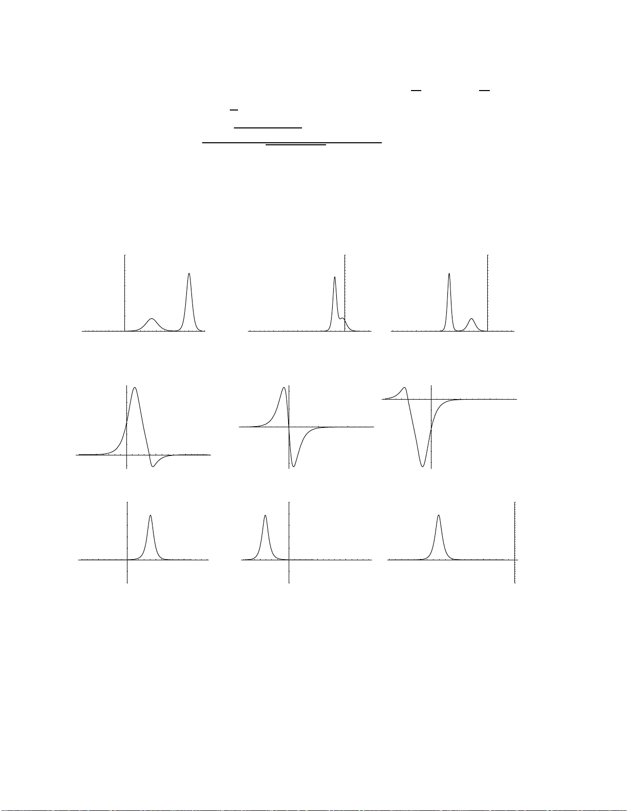
On Camass a-Holm equation with self-consisten t sources and its solutions Y eh ui Huang ∗ , Y uqin Y ao † and Y un b o Zeng ‡ Departmen t of Mathematical Sciences, Tsingh ua Univ ersit y , Beijing, 100 084, P .R. China Abstract Regarded as the integrable generaliza tio n of Camassa-Holm (CH) equation, the CH equa - tion with self-consis tent sources ( CHESCS) is der ived. The Lax representation of the CHESCS is presented. The conserv ation laws for CHESCS a re constr ucted. The p eakon solution, N-soliton, N-cusp on, N-p osito n and N-nega ton solutions o f CHESCS are o btained by using Darb oux trans- formation and the metho d of v ariation of constants. KEYW ORDS: Camassa-Holm equation with self-consisten t sources; Lax represent ation; con- serv a tion la ws; p eak on; s oliton; p ositon; nega ton. 1 In tro duction Camassa-Holm (CH) equation, whic h w as implicitly con tained in the class of multi-Ha miltonian system in trodu ced b y F uc hssteiner and F ok a s 1 and explicitly derived as a shallo w wa ter w a v e equation b y Camassa and Holm 2 , 3 , has the form u t + 2 ω u x − u xxt + 3 uu x = 2 u x u xx + uu xxx , (1.1) where u = u ( x, t ) is the fluid v elo cit y in the x direction an d the constant 2 ω is related to the cr itical shallo w w ate r w a v e sp eed. Let q = u − u xx + w , w e ha v e the follo wing equiv ale nt equation 4 . q t + 2 u x q + uq x = 0 . (1.2) It w as sho wn by Camassa and Holm that this equation s hares m ost of the prop erties of the inte grable system of KdV t yp e 2 , 3 . It p ossesses Lax pair form alism and the b i-hamiltonian structur e. When w > 0, the CH equation h as smo oth solitary wa v e solutions. When w − → 0, these solutions b ecome piecewise smo oth and hav e cusps at th eir p eaks. T h ese kind of solutions are weak solutions of (1.2) with ω = 0 and are called ”p eak ons”. Since the w orks of Camassa and Holm, this equ ation has ∗ Corresponding author: Y ehui Huang, T el: +86-13810446 869, e-mail: huangyh@mails.tsingh ua.edu.cn † yuqinya o@mail.tsingh ua.edu.cn ‡ yzeng@math.tsinghua.edu.cn 1 b ecome a well-kno wn example of in tegrable sys tems and has b een studied from m any k in ds of views 4 − 12 . Soliton equations with self-consistent sources (SESCS) h a v e attracted muc h atten tion in recen t y ears. They are imp ortant in tegrable mod els in man y fields of ph ysics, suc h as h ydro d ynamics, state physics, p lasma ph ysics, etc 13 − 25 . F or example, the KdV equation with self-consistent sources describ es th e in teraction of long and short capillary-gra vity w a v es 13 . Th e nonlinear Sc hr ¨ o dinger equation w ith self-consisten t sour ces represents the n onlinear interact ion of an electrostatic high- frequency wa v e with th e ion acoustic wa v e in a t w o comp onent homogeneous p lasma 18 . The KP equation with self-co nsistent sources d escrib es the in teraction of a long wa v e with a short w av e pac k et pr opagating on the x - y plane at some angle to eac h other 15 . The S ESCS w ere fi rstly studied by Melnik o v 13 − 15 . A systematic wa y to construct the soliton equations with self-consisten t sources and their zero-curv atur e representa tions is p rop osed 21 − 24 . The p roblem of findin g soliton solutions or other s p ecific solutions for SESCS h as b een considered in the past b y many authors 13 − 25 . The present pap er falls in th at line of the wo rk on th e CH equation concernin g with establish- ing the many facts of its completely integrable charact er, aiming at the integrable generalization of CH equation b y derivin g the Camassa-Holm equ ation with self-co nsistent sources (CHESCS) and findin g its solutions. W e first construct the CHESCS by us ing the approac h presented in the reference 21 − 24 . The Lax pair of the CHES CS is obtained, which means that the CHES CS is Lax in tegrable and can b e viewe d as int egrable generalization of CH equation. S ince the C H equation describ es shallo w wate r wa ve and the S ESCS s in general describ e the interacti on of different soli- tary wa v es, it is reasonable to sp eculate on the p oten tial app lication of CHESCS, that is, CHESCS ma y describ e the in teraction of differen t solitary w a v es in shallo w wate r. It was p ointed out 26 , 27 that S ESCS can b e regarded as soliton equ ations w ith non-homogeneous terms, and acc ordingly prop osed to lo ok for explicit solutions b y using the metho d of v ariation of constants. App lying this tec hniqu e to CHESC S w e ha ve b een able to fi nd its p eak on solution. In ord er to find other solutions of CHESCS, we consider the recipro cal transformation 28 , 29 , which relates CH equation to an alternativ e of the asso ciated Camassa-Holm (ACH) equation, and pr op ose the recipro cal trans- formation, wh ic h relates the CHES CS to asso ciated CHESC S (ACHESCS). By using the Darb oux transformation (DT), one can find the n-soliton and n-cusp on solution 8 , 9 as well as p ositon and negaton solution of alternativ e ACH equation. Th en b y means of the metho d of v ariation of con- stan ts, w e can obtain th e N-soliton, N-cusp on, N-p ositon and N-negaton s olution for A CHESCS . Finally , using the inv erse recipro cal transformation, w e obtain the N-soliton, N-cusp on, N-p ositon and N-negaton solution of CHESCS . This pap er is organized as f ollo ws. In sectio n 2, we present h o w to derive the CHESCS and its Lax r epresent ation. In section 3, the conserv ation la ws of the CHES CS are constru cted. In section 4, the p eak on solution is obtained. In section 5, we consider the recipro cal transformation for CH equation and CHES CS, resp ectiv ely . In section 6, by using the DT, w e find the solution for alternativ e A CH equation, then b y using the metho d of v ariation of constants and inv er s e recipro cal transformation, w e obtain the N-soliton, N-cusp on, N-p ositon and N-negaton solution for C HESCS. In section 7, the conclusion is presented. 2 2 The CHESCS and its L ax pair 2.1 The CHESCS The Lax p air for CH equation (1.2) is giv en by 2 ϕ xx = ( λq + 1 4 ) ϕ, (2.1a) ϕ t = ( 1 2 λ − u ) ϕ x + 1 2 u x ϕ. (2.1b) It is not difficult to find that δ λ δ q = − λϕ 2 . (2.2) The CH equation p ossesses bi-hamiltonian stru cture 2 q t = − J δ H 0 δ q = − K δ H 1 δ q , (2.3) where K = − ∂ 3 + ∂ , J = ∂ q + q ∂ , H 0 = 1 2 Z u 2 + u 2 x dx, H 1 = 1 2 Z u 3 + uu 2 x dx. According to the approac h prop osed in the reference 21 − 24 , the CHESCS is defined as follo ws q t = − J ( δ H 0 δ q − 2 N X j =1 δ λ j δ q ) = − ( q ∂ + ∂ q )( u + 2 N X j =1 λ j ϕ 2 j ) = − 2 q u x − uq x + N X j =1 ( − 8 λ j q ϕ j ϕ j x − 2 λ j q x ϕ 2 j ) , (2.4a) ϕ j,xx = ( λ j q + 1 4 ) ϕ j , j = 1 , · · · , N , (2.4b) whic h has a equiv alen t form b y using (2.4b) q t = − 2 q u x − uq x + N X j =1 [( ϕ 2 j ) x − ( ϕ 2 j ) xxx ] , (2.5a) ϕ j,xx = ( λ j q + 1 4 ) ϕ j , j = 1 , · · · , N , (2.5b) 3 2.2 The Lax represen tation of t he CHESCS Based on the Lax p air of the CH equation (2.1), w e may assume the Lax repr esen tation of the CHESCS (2.4) or (2.5) has the form ϕ xx = ( λq + 1 4 ) ϕ, (2.6a) ϕ t = − 1 2 B x ϕ + B ϕ x , (2.6b) B = 1 2 λ − u + N X j =1 α j f ( ϕ j ) λ − λ j + N X j =1 β j f ( ϕ j ) , (2.6c) where f ( ϕ j ) is undetermin ed f unction of ϕ j . Th e compatibilit y condition of (2.6a) and (2.6b) giv es λq t = LB + λ (2 B x q + B q x ) , (2.7) where L = − 1 2 ∂ 3 + 1 2 ∂ . Then (2.6) and (2.7) yields λq t = − 1 2 N X j =1 α j λ − λ j [ f ′′′ ϕ 3 j x + 3( f ′′ ϕ j − f ′ )( λ j q + 1 4 ) ϕ j x + λ j q x ( f ′ ϕ j − 2 f )] +[ − 2 q u x − uq x + N X j =1 β j (2 q ϕ j x f ′ + q x f )] λ − 1 2 N X j =1 β j [ f ′′′ ϕ 2 j x + (3 f ′′ ϕ j + f ′ ) × ( λ j q + 1 4 ) ϕ j x + λ j f ′ q x ϕ j − f ′ ϕ j ] + N X j =1 α j ( q x f + 2 q f ′ ϕ j x ) . (2.8) Here f ′ denotes the p artial deriv ativ e of the fun ction f with resp ect to th e v ariable ϕ j . In order to determine f , α j and β j , w e compare the co efficients of 1 λ − λ j , λ and λ 0 , resp ectiv ely . W e first observ e the coefficients of 1 λ − λ j , th en the coefficien ts of ϕ 3 j x , ϕ j x and other terms giv es rise to, resp ectiv ely f ′′′ = 0 , f ′′ ϕ j − f ′ = 0 , f ′ ϕ j − 2 f = 0 , whic h leads to f = bϕ 2 j . Sub s tituting f = bϕ 2 j in to the co efficien ts of λ in (2.8) giv es q t = − 2 q u x − uq x + 4 q N X j =1 β j bϕ j ϕ j x + q x N X j =1 β j bϕ 2 j . Comparing the ab ov e equation and (2.4a), we can determine b = − 2 , β j = λ j . Substituting f = − 2 ϕ 2 j , and β j = λ j in to the co efficien ts of λ 0 in (2.8), we obtain α j = λ 2 j . 4 Th us w e obtain the L ax pair of th e CHES CS (2.5) ϕ xx = ( 1 4 + λq ) ϕ, (2.9a) ϕ t = u x 2 ϕ + ( 1 2 λ − u ) ϕ x + 2 N X j =1 λλ j ϕ j λ − λ j ( ϕ j x ϕ − ϕ j ϕ x ) . (2.9b) whic h means that the CHES C S (2.5) is Lax integrable. 3 The infinite conserv ation la ws of the CHESCS With the help of th e Lax r epresen tation of the C HES CS, we could find the conserv ation la ws f or the CHES CS b y a w ell-kno wn metho d. First we assume that q , u , ϕ j and its deriv ativ es tend to 0 when | x | → ∞ . Set Γ = ϕ x ϕ , (3.1) then the identi t y ∂ ∂ t ( ∂ ln ϕ ∂ x ) = ∂ ∂ x ( ∂ ln ϕ ∂ t ) together with (2.10) implies that CHESC S h as the follo wing conserv ation la w: ∂ ∂ t (Γ) = ∂ ∂ x ( ϕ t ϕ ) = ∂ ∂ x ( 1 2 u x + 2 N X j =1 λλ j λ − λ j ϕ j ϕ j x + (( 1 2 λ − u ) − 2 N X j =1 λλ j λ − λ j ϕ 2 j )Γ) (3.2) . Using (2.10a ) giv es r ise to Γ x = 1 4 + q λ − Γ 2 . (3.3) Let Γ = ∞ X m =0 µ m λ 1 − m 2 , (3.4) then µ m is the densit y of conserv ation la ws. Define 1 2 u x + 2 N X j =1 λλ j λ − λ j ϕ j ϕ j x + (( 1 2 λ − u ) − 2 N X j =1 λλ j λ − λ j ϕ 2 j )Γ = ∞ X m =0 F m λ 1 − m 2 (3.5) It is found that the d ensit y of the conserv ation la ws µ m and the flux of the conserv ation la ws F m satisfy the follo wing r ecursion relation: µ 0 = √ q , µ 1 = − 1 4 q x q , µ 2 = 1 32 ( 4 √ m + m 2 x m 5 / 2 − ( 4 m x m 3 / 2 ) x ) , µ m = − µ m − 1 ,x − P m − 1 i =1 µ i µ m − 1 − i 2 µ 0 , m ≥ 3 , (3.6) 5 F 0 = ( − u − 2 N X j =1 λ j ϕ 2 j ) √ q , F 1 = ( u + 2 N X j =1 λ j ϕ 2 j ) q x 4 q + 1 2 u x + 2 N X j =1 λ j ϕ j ϕ j x , F 2 m = m X i =0 ( − u ( i ) − 2 N X j =1 λ i +1 j ϕ 2 j ) µ 2 m − 2 i , m ≥ 1 , F 2 m +1 = m X i =0 ( u ( i ) + 2 N X j =1 λ i +1 j ϕ 2 j ) µ 2 m − 2 i +1 + 2 N X j =1 λ m +1 j ϕ j ϕ j x , m ≥ 1 , (3.7) where u (0) = u , u (1) = 1, u ( i ) = 0 , i > 1. After some calculations we can fin d the first few conserv ed quantiti es giv en by µ 0 , µ 2 and µ 4 are as follo ws H − 1 = Z √ q dx, (3.8a) H − 2 = − 1 16 Z ( 4 √ q + q 2 x q 5 / 2 ) dx, (3.8b) H − 3 = − Z ( 1 32 q 3 / 2 + 5 q 2 x 64 q 7 / 2 + q 2 xx 32 q 7 / 2 − 35 q 4 x 512 q 11 / 2 ) dx. (3.8c) The corresp ond in g flux of the conserv ation laws are G − 1 = ( − u − 2 N X j =1 λ j ϕ 2 j ) √ q , (3.9a) G − 2 = (1 + 2 N X j =1 λ 2 j ϕ 2 j ) √ q + ( u + 2 N X j =1 λ j ϕ 2 j )( 1 16 ( 4 √ q + q 2 x q 5 / 2 ) − ( q x 4 q 3 / 2 ) x ) , (3.9b) G − 3 = ( − u − 2 N X j =1 λ j ϕ 2 j )( 1 32 q 3 / 2 + 5 q 2 x 64 q 7 / 2 + q 2 xx 32 q 7 / 2 − 35 q 4 x 512 q 11 / 2 ) + 1 16 (1 + 2 N X j =1 λ 2 j ϕ 2 j )( 4 √ q + q 2 x q 5 / 2 ) + 2 N X j =1 λ 3 j ϕ 2 j √ q . (3.9c) As the space part of the Lax Pair of the CHESCS is the same as that of CH equation, the densities of th e conserv ation laws of the CHESCS are the same as those of the Camassa-Holm equation 12 . As the time part of the Lax pair is d ifferen t, the fluxs of the conserv ation la ws for CH equation and CHESCS are differen t. 4 One p eak on solution of the CHESCS The CH equation (1.2) has p eak on solutions 2 u = ce −| x − ct + α | , (4.1) 6 where α is an arbitrary constan t. Th e corresp onding eigenfunction of (2.1) is ϕ = β e − 1 2 | x − ct + α | , (4.2 ) where β is an arbitrary constan t. Since the C HESCS (2.5) can b e considered as the C H equation (1.2) w ith non-homogeneous terms, we m a y use th e metho d of v ariation of constan ts to fi n d the p eak on solution of CHES CS from the p eak on solution (4.1) and (4.2). T aking α and β in (4.1) and (4.2) to b e time-dep enden t α ( t ) and β ( t ) and requiring that u = ce −| x − ct + α ( t ) | , (4.3a) ϕ = β ( t ) e − 1 2 | x − ct + α ( t ) | (4.3b) satisfy the CHESCS (2.5) for N = 1. W e find that c = 1 λ , α ( t ) can b e an arbitrary fu nction of t and β ( t ) = p α ′ ( t ) c . So we ha v e th e one p eak on solution f or (2.4) with N = 1, λ 1 = λ = 1 c u = ce −| x − ct + α ( t ) | (4.4a) ϕ = p α ′ ( t ) ce − 1 2 | x − ct + α ( t ) | (4.4b) The one p eak on of the C HESCS also has a cusp at its p eak, lo cate d at x = ct − α ( t ). W e n ote that for the one p eak on solution of the CH equation, the solution trav els with sp eed c and has a cusp at its p eak of h eigh t c , f or the CHES CS, the cusp is still at its p eak of height c , but the sp eed c − α ( t ) t of the w a v e is n o longer a constan t. 5 A recipro cal transformation for the CHESCS Let r = √ q , by the r ecipro cal transformation 4 , 28 , 29 dy = r dx − ur ds, ds = dt, and denoting f = r − 1 2 φ , the Lax p air (2.1) of CH equation is transformed to the f ollo wing sys tem φ y y = ( λ + Q + 1 4 ω ) φ, (5.1a) φ s = 1 2 λ ( r φ y − 1 2 r y φ ) , (5.1b) where Q = − 1 4 ( r y r ) 2 + r y y 2 r + 1 4 r 2 − 1 4 ω . (5.2) The compatibilit y condition of (5.1a) and (5.1b) giv es an alternativ e of the asso ciated CH (ACH) equation Q s = r y , (5.3a) − 1 4 ω r y + 1 4 r y y y − 1 2 Q y r − Qr y = 0 . (5.3b) 7 W e now consider the recipro cal transf ormation for the C HESCS (2.5). (2.5a) giv es r t = − ( r u ) x − 2 N X j =1 λ j ( r ϕ 2 j ) x . (5.4) (5.4) sho ws that the 1-form ω = r dx − ( r u + 2 N X j =1 λ j r ϕ 2 j ) dt (5.5) is closed, so we can define a r ecipro cal transf orm ation ( x, t ) → ( y , s ) by the r elation dy = r dx − ( r u + 2 N X j =1 λ j r ϕ 2 j ) ds, ds = dt, (5.6) and w e hav e ∂ ∂ x = r ∂ ∂ y , ∂ ∂ t = ∂ ∂ s − ( r u + 2 N X j =1 λ j r ϕ 2 j ) ∂ ∂ y . (5.7) Denoting ϕ = r − 1 2 ψ , ϕ j = r − 1 2 ψ j and usin g (5.2), the Lax pair (2.9) of CHESCS (2.5) is corre- sp ond ingly rewritten as ψ y y = ( λ + Q + 1 4 ω ) ψ , (5.8a) ψ s = 1 2 λ ( r ψ y − 1 2 r y ψ ) + 2 N X j =1 λ 2 j ψ j λ − λ j ( ψ j y ψ − ψ j ψ y ) . (5.8b) The compatibilit y condition of (5.8a) and (5.8b) leads to an asso ciated CHES CS (ACHESCS) Q s = r y − 8 N X j =1 λ 2 j ψ j ψ j y , (5.9a) − 1 4 ω r y + 1 4 r y y y − 1 2 Q y r − Qr y = 0 , (5.9b) ψ j yy = ( λ j + Q + 1 4 ω ) ψ j , j = 1 , 2 , · · · , N . (5.9c) The Eqs.(5.9) can b e regarded as the Eqs.(5.3) with self-consisten t sources. I n order to obtain th e solutions of the CHESC S (2.5), w e h a v e to get the relation of th e v ariables ( y , s ) and the v ariables ( x, t ). F rom the recipro cal transform ation, we h av e ∂ x ∂ y = 1 r , ∂ x ∂ s = u + 2 N X j =1 λ j ϕ 2 j . (5.10) By making u se of the compatibilit y of th e ab o ve tw o equations, we ha v e x ( y , s ) = Z 1 r dy . (5.11) 8 The solutions of the CHESC S (2.5) with resp ect to the v ariables (y ,s) are giv en by q = r 2 ( y , s ) , ϕ j ( y , s ) = ψ j √ r , (5.12a ) u ( y , s ) = r 2 − r y s + r y r s r − 2 r r y N X j =1 λ j ( ϕ 2 j ) y − 2 r 2 N X j =1 λ j ( ϕ 2 j ) y y − ω , (5.12b) x ( y , s ) = Z 1 r dy . (5.12c ) W e now pro v e (5.12b). F rom q = u − u xx + ω and the recipro cal transform ation (5.7), we h a v e u = q + r r y u y + r 2 u y y − ω . (5.13) By using the recipro cal transformation (5.7 ), (5.4 ) giv es rise to u y = − r s r 2 − 2 N X j =1 λ j ( ϕ 2 j ) y . (5.14) Substituting (5.14) and (5.2) into (5.13) leads to (5.12b). 6 The solutions for the CHESCS Notice that Q = 0, r = √ ω is the solution of (5.2) and (5.3). Let the fu nctions φ 0 ( y , s, λ ), Ψ 1 ( y , s, λ 1 ), · · · , Ψ n ( y , s, λ n ) b e differen t solutions of (5.1) with Q = 0, r = √ ω and the co rre- sp ond ing λ and λ = λ 1 , · · · , λ n , resp ectiv ely . W e construct t w o W ronskian determinants f rom these functions W 1 = W (Ψ 1 , · · · , Ψ ( m 1 ) 1 , Ψ 2 , · · · , Ψ ( m 2 ) 2 , · · · , Ψ n , · · · , Ψ ( m n ) n ) , (6.1a) W 2 = W (Ψ 1 , · · · , Ψ ( m 1 ) 1 , Ψ 2 , · · · , Ψ ( m 2 ) 2 , · · · , Ψ n , · · · , Ψ ( m n ) n , φ 0 ) , (6.1b) where m i ≥ 0 are given num b ers and Ψ ( i ) j = ∂ i Ψ j ( y, s ,λ ) ∂ λ i | λ = λ j . Based on th e generalized Darb oux transf ormation for K dV hierarch y 30 and using (5.3a), the follo win g generalized Darb oux trans formation of (5.1) is v alid 4 , 30 , 31 Q ( y , s ) = − 2 ∂ 2 ∂ y 2 log W 1 , (6.2a) r ( y , s ) = √ ω − 2 ∂ 2 ∂ y ∂ s log W 1 , (6.2b) φ ( y , s, λ ) = W 2 W 1 , (6.2c) namely Q ( y , s ), r ( y , s ) and φ ( y , s, λ ) satisfy (5.1), (5.2) and (5.3). 9 6.1 The m ult isolit on solutions T ak e Ψ i and Φ i b e the solutions of Eq.(5.1) with Q = 0 , r = √ ω and λ i = k 2 i − 1 4 ω < 0, or 4 ω k 2 i − 1 < 0, (0 < k 1 < k 2 < · · · < k n ) as follo ws Ψ i = coshξ i , i is an odd num ber , (6.3a) Ψ i = sin hξ i , i is an ev en number. (6.3b) Φ i = e ξ i (6.4) where henceforth ξ i = k i [ y + 2 ω 3 / 2 s 4 ω k 2 i − 1 + α i ] . (6.5) By u sing Darb oux transf orm ation (6.2) w ith m 1 = · · · = m n = 0, the n -soliton solution Q ( y , s ) and r ( y , s ) of (5.3) and the corresp onding eigenfunction φ i ( y , s, λ i ) of (5.1) with λ i = k 2 i − 1 4 ω is give n b y Q ( y , s ) = − 2[ l og W (Ψ 1 , Ψ 2 , · · · , Ψ n )] y y , (6.6a) r ( y , s ) = √ ω − 2[ l og W (Ψ 1 , Ψ 2 , · · · , Ψ n )] y s , (6.6b) φ i ( y , s, λ i ) = W (Ψ 1 , Ψ 2 , · · · , Ψ n , Φ i ) W (Ψ 1 , Ψ 2 , · · · , Ψ n ) . (6.6c) When n = 1 and 4 k 2 1 ω − 1 < 0, (6.6) giv es rise to one soliton solution for (5.3) and the corresp onding eigenfunction of (5.1) with λ 1 = k 2 1 − 1 4 ω 8 , 9 Q ( y , s ) = − 2 k 2 1 sech 2 ξ 1 , r ( y , s ) = √ ω − 4 k 2 1 ω 3 2 sech 2 ξ 1 4 k 2 1 ω − 1 , (6 .7a) φ 1 = k 1 sechξ 1 . (6.7b) Since Eq .(5.9 ) can b e considered to b e Eq.(5.3) with non-homogeneous terms and φ 1 satisfies (5.1a) with λ = λ 1 , we ma y app ly the metho d of v ariation of constant to fi nd the solutions of the CHESCS (5.9 ) by usin g the solution (6.7) of ACH equation (5.3) and corresp onding eigenfunction. T aking α 1 in (6.5) to b e time-dep end en t fu nctions α 1 ( s ) and r equiring that ¯ Q ( y , s ) = − 2 k 2 1 sech 2 ¯ ξ 1 , ¯ r ( y , s ) = √ ω − 4 k 2 1 ω 3 2 sech 2 ¯ ξ 1 4 k 2 1 ω − 1 , (6 .8a) ¯ ψ 1 = β 1 ( s ) k 1 sech ¯ ξ 1 (6.8b) satisfy the system (5.9) for N = 1, henceforth, we denote ¯ ξ i = k i [ y + 2 ω 3 / 2 s 4 ω k 2 i − 1 + α i ( s )] . (6.9) W e fin d that α 1 ( s ) can b e an arb itrary f unction of s and β 1 ( s ) = 2 ω 1 − 4 k 2 1 ω q 2 α ′ 1 ( s ) . (6.10) 10 So the one-soliton solution of the CHESC S (2.5) with N = 1 and λ 1 = k 2 1 − 1 4 ω < 0 is obtained with resp ect to the v ariables ( y , s ) from (5.12) q ( y , s ) = ω (1 − 4 k 2 1 ω sech 2 ¯ ξ 1 4 k 2 1 ω − 1 ) 2 , (6.11a ) u ( y , s ) = 8 k 2 1 ω 2 sech 2 ¯ ξ 1 (1 − 4 k 2 1 ω )(1 − 4 k 2 1 ω + 4 k 2 1 ω sech 2 ¯ ξ 1 ) , (6.11b) ϕ 1 ( y , s ) = 2 p 2 α ′ 1 ( s ) k 1 ω sech ¯ ξ 1 q √ ω (1 − 4 k 2 1 ω )(1 − 4 k 2 1 ω + 4 k 2 1 ω sech 2 ¯ ξ 1 ) , (6.11c ) x ( y , s ) = y √ ω − 2 ln 1 − 2 k 1 √ ω tanh ¯ ξ 1 1 + 2 k 1 √ ω tanh ¯ ξ 1 . (6.11d) The requirement 4 k 2 1 ω − 1 < 0 guarantee s the nonsingularit y of solution (6.11). In Fig 1, w e plot the single soliton solution of u and ϕ 1 . -60 -40 -20 20 40 60 80 x 0.0002 0.0004 0.0006 0.0008 0.001 u -60 -40 -20 20 40 60 80 x 0.05 0.1 0.15 0.2 j 1 Figure 1. Single soliton solutions for u and the eigenfunction ϕ 1 when w = 0 . 01 , k 1 = 1 , α 1 ( s ) = 4 s, s = 2 . When n = 2, λ 1 = k 2 1 − 1 4 ω < 0, λ 2 = k 2 2 − 1 4 ω < 0, we hav e Ψ 1 = coshξ 1 , Ψ 2 = sin hξ 2 , (6.12a ) Φ 1 = e ξ 1 , Φ 2 = e ξ 2 , (6.12b) W 1 (Ψ 1 , Ψ 2 ) = k 2 coshξ 2 coshξ 1 − k 1 sinhξ 2 sinhξ 1 , (6.12c ) W 2 (Ψ 1 , Ψ 2 , Φ 1 ) = k 2 ( k 2 2 − k 2 1 ) sinhξ 1 , (6.1 2d) W 2 (Ψ 1 , Ψ 2 , Φ 2 ) = k 1 ( k 2 1 − k 2 2 ) coshξ 2 , (6.12e ) (6.12f ) Then (6.6) w ith n = 2 giv es rise to tw o soliton solution for (5.3) and the corresp ondin g eigenfunction of (5.1). I n the same w a y as we d id on the one-soliton solution, we can apply the metho d of v ariation of constan ts to get the tw o soliton solution of the A CHESCS (2.9) whic h together with (5.12) yields 11 to th e t w o soliton solution f or C HESCS (2.5) with N = 2 , λ 1 = k 2 1 − 1 4 ω , λ 2 = k 2 2 − 1 4 ω r ( y , s ) = √ ω − 2[ l og W 1 (Ψ 1 , Ψ 2 )] y s | ξ i = ¯ ξ i , (6 .13a) ψ i = 2 ω p ( − 1) i +1 2 α ′ i ( s ) W 2 (Ψ 1 , Ψ 2 , Φ i ) (1 − 4 k 2 i ω ) r Q j 6 = i ( k 2 j − k 2 i ) W 1 (Ψ 1 , Ψ 2 ) | ξ i = ¯ ξ i , i = 1 , 2 . (6.13b) In Fig 2 w e plot the in teractions of t w o soliton solution for u and ϕ 1 , ϕ 2 , wh ic h is sh o wn that u is elastic collision. -40 -20 20 40 60 80 100 x 0.001 0.002 0.003 0.004 0.005 u -200 -150 -100 -50 50 x 0.001 0.002 0.003 0.004 0.005 u -200 -150 -100 -50 50 x 0.001 0.002 0.003 0.004 0.005 u (a)s=-2 (b)s=1 (c)s=2 -50 50 100 x -0.02 0.02 0.04 0.06 0.08 0.1 0.12 j 1 -50 50 100 x -0.1 -0.05 0.05 0.1 j 1 -50 50 100 x -0.12 -0.1 -0.08 -0.06 -0.04 -0.02 0.02 j 1 (d)s=-1 (e)s=0 (f )s=1 -50 50 100 x -0.2 -0.1 0.1 0.2 0.3 0.4 0.5 j 2 -50 50 100 x -0.2 -0.1 0.1 0.2 0.3 0.4 0.5 j 2 -200 -150 -100 -50 x -0.2 -0.1 0.1 0.2 0.3 0.4 0.5 j 2 (g)s=-1 (h)s=1 (i)s=3 Figure 2. tw o soliton solutions for u and the eigenfunction ϕ 1 , ϕ 2 when w = 0 . 01 , k 1 = 2 , k 2 = 1 , α 1 ( s ) = 2 s, α 2 ( s ) = 4 s. Notice th at the soliton solutions of CHESCS contai ns arbitrary s fun ctions α j ( s ). Th is implies that the in sertion of sources into the CH equation ma y cause the v ariation of the sp eed of soliton. 12 In the same wa y as in the reference 27 , we m a y apply the metho d of v ariation of constan t to find the N-soliton solution of (2.5) with λ i = k 2 i − 1 4 ω > 0 , i = 1 , · · · , N , from (5.12), where r ( y , s ) = √ ω − 2[ l og W 1 (Ψ 1 , Ψ 2 , · · · , Ψ N )] y s | ξ i = ¯ ξ i , (6.14a ) ψ i = 2 ω p ( − 1) i +1 2 α ′ i ( s ) W 2 (Ψ 1 , Ψ 2 , · · · , Ψ N , Φ i ) (1 − 4 k 2 i ω ) r Q j 6 = i ( k 2 j − k 2 i ) W 1 (Ψ 1 , Ψ 2 , · · · , Ψ N ) | ξ i = ¯ ξ i (6.14b) 6.2 The m ult ic usp on solutions T ak e Ψ i and Φ i b e the solutions of Eq.(5.1) when Q = 0 , r = √ ω and λ i = k 2 i − 1 4 ω > 0 (0 < k 1 < k 2 < · · · < k n ), as follo ws Ψ i = sin hξ i , i is an odd number, (6.15a ) Ψ i = coshξ i , i is an ev en number. (6.15b) Φ i = e ξ i , (6.16) where ξ i is giv en by (6.5). The n -cusp on solution Q ( y , s ) and r ( y , s ) of (5.3) an d the corresp ondin g eigenfunction φ i ( y , s, λ i ) of (5.1) with λ i = k 2 i − 1 4 ω is give n by (6.6). When n = 1 and 4 k 2 1 ω − 1 > 0, (6.6) gives rise to one cusp on solution for (5.3) and the corresp ondin g eigenfunction of (5.1) with λ 1 = k 2 1 − 1 4 ω 8 , 9 Q ( y , s ) = 2 k 2 1 csch 2 ξ 1 , r ( y , s ) = √ ω + 4 k 2 1 ω 3 2 csch 2 ξ 1 4 k 2 1 ω − 1 , (6.17a ) φ 1 = − k 1 cschξ 1 . (6.17b) Similarly , we ma y apply the metho d of v ariation of constant to find the solutions of th e A CHESCS (5.9) by using the solution (6.17) of (5.3) and corresp onding eigenfunction. T aking α 1 in (6.5) to b e time-dep end en t fu nctions α 1 ( s ) and r equiring that ¯ Q ( y , s ) = 2 k 2 1 csch 2 ¯ ξ 1 , ¯ r ( y , s ) = √ ω + 4 k 2 1 ω 3 2 csch 2 ¯ ξ 1 4 k 2 1 ω − 1 , (6.18a ) ¯ ψ 1 = β 1 ( s ) k 1 csch ¯ ξ 1 (6.18b) satisfy the system (5.9) for N = 1, w e fin d that α 1 ( s ) can b e an arb itrary f unction of s and β 1 ( s ) = 2 ω 1 − 4 k 2 1 ω q − 2 α ′ 1 ( s ) . (6.19) So the one-cusp on solution of the CHESC S (2.5) with N = 1 and λ 1 = k 2 1 − 1 4 ω > 0 is obtained 13 with resp ect to the v ariables ( y , s ) from (5.12) q ( y , s ) = ω (1 + 4 k 2 1 ω csch 2 ¯ ξ 1 4 k 2 1 ω − 1 ) 2 , (6.20a ) u ( y , s ) = 8 k 2 1 ω 2 csch 2 ¯ ξ 1 (1 − 4 k 2 1 ω )( − 1 + 4 k 2 1 ω + 4 k 2 1 ω csch 2 ¯ ξ 1 ) , (6.20b) ϕ 1 ( y , s ) = 2 p 2 α ′ 1 ( s ) k 1 ω csch ¯ ξ 1 q √ ω (1 − 4 k 2 1 ω )( − 1 + 4 k 2 1 ω + 4 k 2 1 ω csch 2 ¯ ξ 1 ) , (6.20c ) x ( y , s ) = y √ ω + 2 ln 1 − 2 k 1 √ ω coth ¯ ξ 1 1 + 2 k 1 √ ω coth ¯ ξ 1 (6.20d) In Fig 3, w e plot the one-cusp on solution of u , ϕ 1 . -6 -4 -2 2 4 6 x -0.5 -0.4 -0.3 -0.2 -0.1 u -10 -7.5 -5 -2.5 2.5 5 x -1 -0.5 0.5 1 j 1 Figure 3. Single cu sp on solution for u and the eigenfunction ϕ 1 when w = 1 , k 1 = 1 , α 1 ( s ) = − 2 s, s = 2 . Similarly , we can apply the metho d of v ariation of constant to fin d the N-cusp on solution of (2.5) with λ i = k 2 i − 1 4 ω < 0 , i = 1 , · · · , N from (5.12), wh ere r ( y , s ) = √ ω − 2[ l og W 1 (Ψ 1 , Ψ 2 , · · · , Ψ N )] y s | ξ i = ¯ ξ i , (6.21a ) ψ i = 2 ω p ( − 1) i +1 2 α ′ i ( s ) W 2 (Ψ 1 , Ψ 2 , · · · , Ψ N , Φ i ) (1 − 4 k 2 i ω ) r Q j 6 = i ( k 2 j − k 2 i ) W 1 (Ψ 1 , Ψ 2 , · · · , Ψ N ) | ξ i = ¯ ξ i (6.21b) F urther more in the same wa y , we can fnd mixed k 1 -soliton- k 2 -cusp on solution for (2.5) with N = k 1 + k 2 , λ i = k 2 i − 1 4 ω > 0 , i = 1 , · · · , k 1 and λ i = k 2 i − 1 4 ω < 0 , i = K 1 + 1 , · · · , k 1 + k 2 , by using (6.6) and (5.12). 6.3 The m ult ip ositon solutions Let λ = − k 2 − 1 4 ω , λ i = − k 2 i − 1 4 ω , i = 1 , · · · , N , and tak e Ψ i = sin ξ i , i is an odd number, (6.22a ) Ψ i = cosξ i , i is an ev en n umber . (6.22b) 14 Φ i = cosξ i , i is an odd number , (6.23a ) Φ i = sin ξ i , i is an ev en number. (6.23b) where ξ = k ( y − 2 ω 3 / 2 s 4 k 2 ω + 1 ) + N X i =1 N Y j =1 ( k − k j ) 2 α i k − k i , ξ i = ξ | k = k i . F or N = 1, w e hav e Ψ 1 = sin ξ 1 , Ψ (1) 1 = γ 1 cos ξ 1 , (6.24a ) ξ 1 = k 1 ( y − √ ω s 2( k 2 1 + 1 4 ω ) ) . (6.24b) γ 1 = ∂ ξ ∂ k | k = k 1 = α 1 + y + 16 k 2 1 ω 5 / 2 s (1 + 4 k 2 1 ω ) 2 − 2 ω 3 / 2 s 1 + 4 k 2 1 ω , (6.24c ) and W 1 (Ψ 1 , Ψ (1) 1 ) = − k 1 γ 1 + 1 2 sin 2 ξ 1 , (6.25a ) W 2 (Ψ 1 , Ψ (1) 1 , Φ 1 ) = − 2 k 2 1 sin ξ 1 . (6.2 5b) Then the one-p ositon solution of (5.3) and the corresp onding eigenfunction for (5.1) is giv en by (6.2) with N = 1 , m 1 = 1 , Q ( y , s ) = − 2[ l og W 1 ] y y , (6.26a ) r ( y , s ) = √ ω − 2[ l og W 1 ] y s . (6.26b) ψ 1 ( y , s, λ 1 ) = β 1 W 2 W 1 , (6.26c ) where α 1 and β 1 are arbitrary constan ts. -100 -50 50 100 150 x -0.004 -0.003 -0.002 -0.001 0.001 u -150 -100 -50 50 100 150 200 x -0.1 -0.05 0.05 0.1 j 1 Figure 4. one-p ositon solutions for u and t he eigenfunction ϕ 1 when w = 0 . 01 , k 1 = 1 , α 1 ( s ) = − 2 s, s = 2 . 15 By usin g the metho d of v ariation of constan ts, which means we change α 1 and β 1 in to α 1 ( s ) and β 1 ( s ), we obtain th e one-p ositon solution for the CHESCS (2.5) with N = 1 , λ 1 = − k 2 1 − 1 4 ω from (5.12), where ¯ r ( y , s ) = √ ω − 2[ l og W 1 ] y s | γ 1 = ¯ γ 1 , (6.27a ) ¯ ψ 1 ( y , s ) = 2 ω p − α ′ 1 ( s ) k 1 (1 + 4 k 2 1 ω ) W 2 W 1 | γ 1 = ¯ γ 1 , (6.27b) ¯ γ 1 = α 1 ( s ) + y + 16 k 2 1 ω 5 / 2 s (1 + 4 k 2 1 ω ) 2 − 2 ω 3 / 2 s 1 + 4 k 2 1 ω . (6.27c) where α 1 ( s ) is an arbitrary fu n ction of s . In Fig 4, w e plot the one-p ositon solution of u and ϕ 1 . The p ositon solution of CHESCS is long-range analogue of soliton and is slo wly decreasing, oscillati ng solution 31 . In th e same wa y w e can find N-p ositon solution for (2.5). F or a detailed discussion on p ositon solution we refer to the r eferen ce 31 . F or N , we ha ve Ψ (1) i = γ i cos ξ i , i is an odd number , (6.28a) Ψ (1) i = − γ i sin ξ i , i is an ev en num ber . (6.28b) where γ i = ∂ ξ ∂ k | k = k i = Y j 6 = i ( k i − k j ) 2 α i + y + 16 k 2 i ω 5 / 2 s (1 + 4 k 2 i ω ) 2 − 2 ω 3 / 2 s 1 + 4 k 2 i ω . W e fin d that W 1 = W (Ψ 1 , Ψ (1) 1 , · · · , Ψ N , Ψ (1) N ) , (6.29a ) φ i = W (Ψ 1 , Ψ (1) 1 , · · · , Ψ N , Ψ (1) N , Φ i ) , (6.29b) and the N-p ositon solution of (5.3) and the corresp onding eigenfunction for (5.1) is give n by Q ( y , s ) = − 2[ l og W 1 ] y y , (6.30a ) r ( y , s ) = √ ω − 2[ l og W 1 ] y s . (6.30b) ψ j ( y , s, λ i ) = β i W 2 W 1 , i = 1 , · · · , N , (6.30c ) where α i and β i are arbitrary constan ts. By using the metho d of v ariation of constan ts, w e obtain th e N-p ositon solution for the CHES CS (2.5) from (5.12), where ¯ r ( y , s ) = √ ω − 2[ l og W 1 ] y s | γ i = ¯ γ i , (6.31a ) ¯ ψ i ( y , s ) = 2 ω k i (1 + 4 k 2 i ω ) 1 Q j 6 = i ( k j + k i ) q ( − 1) α ′ i ( s ) W 2 W 1 | γ i = ¯ γ i , (6.31b) ¯ γ i = Y j 6 = i ( k i − k j ) 2 α i ( s ) + y + 16 k 2 i ω 5 / 2 s (1 + 4 k 2 i ω ) 2 − 2 ω 3 / 2 s 1 + 4 k 2 i ω . (6.31c ) where α i ( s ) are arbitrary fun ctions of s . 16 6.4 The m ult inegaton solutions Let λ = k 2 − 1 4 ω > 0, λ i = k 2 i − 1 4 ω > 0 , i = 1 , · · · , N , and tak e Ψ i = sin hξ i , i is an odd number, (6.32a ) Ψ i = coshξ i , i is an ev en number. (6.32b) Φ i = e ξ i , (6.33) where ξ = k ( y + 2 ω 3 / 2 s 4 k 2 ω − 1 ) + N X i =1 N Y j =1 ( k − k j ) 2 α i k − k i , ξ i = ξ | k = k i , then w e ha ve Ψ 1 = sin h ξ 1 , Ψ (1) 1 = γ 1 cosh ξ 1 , ( 6.34a) ξ 1 = k 1 ( y + √ ω s 2( k 2 1 − 1 4 ω ) ) . (6.34b) γ 1 = α 1 + y + − 16 k 2 1 ω 5 / 2 s (4 k 2 1 ω − 1) 2 + 2 ω 3 / 2 s 4 k 2 1 ω − 1 , (6.34c ) and W 1 (Ψ 1 , Ψ (1) 1 ) = − k 1 γ 1 + 1 2 sinh 2 ξ 1 , (6.35a) W 2 (Ψ 1 , Ψ (1) 1 , Φ 1 ) = 2 k 2 1 sinh ξ 1 , (6.35b) Then th e one-negaton solution of (5.3) and the corresp onding eigenfunction for (5.1) is given b y Q ( y , s ) = − 2[ l og W 1 ] y y , (6.36a ) r ( y , s ) = √ ω − 2[ l og W 1 ] y s . (6.36b) φ 1 ( y , s, λ 1 ) = β 1 W 2 W 1 , (6.36c ) where α and β are arbitrary constants. By using the metho d of v ariation of constan ts, we obtain the one-negat on solution for the CHESCS (2.5) with N = 1 , λ 1 = k 2 1 − 1 4 ω from (5.12), where ¯ r ( y , s ) = √ ω − 2[ l og W 1 ] y s | γ 1 = ¯ γ 1 , (6.37a) ¯ ψ 1 ( y , s ) = 2 ω p α ′ 1 ( s ) k 1 (4 k 2 1 ω − 1) W 2 W 1 | γ 1 = ¯ γ 1 , (6.37b) ¯ γ 1 = α 1 ( s ) + y + − 16 k 2 1 ω 5 / 2 s (4 k 2 1 ω − 1) 2 + 2 ω 3 / 2 s 4 k 2 1 ω − 1 . (6.37c ) where α ( s ) is an arbitrary fu nction of s . In Fig 5, w e plot the one-negaton solution of u and ϕ 1 . 17 -40 -20 20 40 60 80 100 x -0.01 -0.008 -0.006 -0.004 -0.002 u -50 50 100 150 x -0.05 0.05 0.1 j 1 Figure 5. one-negaton solution for u and the eigenfunction ϕ 1 when w = 0 . 01 , k 1 = 1 , α 1 ( s ) = 2 s, s = 2 . Similarly , we can fi nd N-negaton s olution for CHES CS (2.5) w ith λ i = k 2 i − 1 4 ω , i = 1 , · · · , N . F or N , we h a v e Ψ (1) i = γ i cosh ξ i , i is an odd number , (6.38 a) Ψ (1) i = γ i sinh ξ i , i is an ev en number . (6.38b) where γ i = ∂ ξ ∂ k | k = k i = Y j 6 = i ( k i − k j ) 2 α i + y + − 16 k 2 i ω 5 / 2 s (4 k 2 i ω − 1) 2 + 2 ω 3 / 2 s 4 k 2 i ω − 1 . W e fin d that W 1 = W (Ψ 1 , Ψ (1) 1 , · · · , Ψ N , Ψ (1) N ) , (6.39a ) φ i = W (Ψ 1 , Ψ (1) 1 , · · · , Ψ N , Ψ (1) N , Φ i ) , (6.39b) and the N-negaton solution of (5.3) and the corresp onding eigenfun ction f or (5.1) is give n by Q ( y , s ) = − 2[ l og W 1 ] y y , (6.40a ) r ( y , s ) = √ ω − 2[ l og W 1 ] y s . (6.40b) ψ j ( y , s, λ i ) = β i W 2 W 1 , i = 1 , · · · , N , (6.40c ) where α i and β i are arbitrary constan ts. By using the metho d of v ariation of constant s, w e obtain the N-negaton solution for the CHESCS (2.5) from (5.12), wher e ¯ r ( y , s ) = √ ω − 2[ l og W 1 ] y s | γ i = ¯ γ i , (6.41a) ¯ ψ i ( y , s ) = 2 ω k i (4 k 2 i ω − 1) 1 Q j 6 = i ( k j + k i ) q α ′ i ( s ) W 2 W 1 | γ i = ¯ γ i , (6.41b) ¯ γ i = Y j 6 = i ( k i − k j ) 2 α i ( s ) + y + − 16 k 2 i ω 5 / 2 s (4 k 2 i ω − 1) 2 + 2 ω 3 / 2 s 4 k 2 i ω − 1 . (6.41c ) where α i ( s ) are arbitrary fun ctions of s . 7 Conclusion The CHESCS and its Lax representat ion are derived. Conserv ation laws are constructed. It is reasonable to s p eculate on the p otren tial application of CHESCS , that is, CHES C S ma y describ e 18 the int eraction of different solitary wa v es in s hallo w wa ter. Since SES CS can b e regarded as soliton equations with non-homogeneous terms , w e lo ok for explicit solutions b y usin g the metho d of v ariation of constan ts. By considering a recipro cal transformation, w hic h r elates CH equ ation to an alternativ e of A CH equation, we p rop ose a similar recipro cal tr ansformation, which relates the CHESCS to A CHESCS. By usin g the Darb oux transformation, one can find the n-soliton and n- cusp on solution as well as n-p ositon and n -negaton solution of alternativ e A C H equ ation. Th en b y means of th e metho d of v ariation of constants, we can obtain N-soliton, N-cusp on, N-p ositon and N-negaton solutions of the ACHESCS. Finally , us in g the in v erse recipro cal transform ation, we obtain N-soliton, N-cusp on, N-p ositon and N-negaton solutions of the C HESCS. Ac kno wledgemen ts This wo rk wa s su p p orted by th e National Basic Research Pr ogram of Ch ina (973 p rogram) (2007 CB814800) , Chin a P ostdo ctoral Science F oun dation fun ded pro ject (2008043 0420) and the National Science F oundation of Ch ina (Grant no 10801083 ). Reference 1 B. F uc hssteiner and A.S. F ok as, Physica D 4 , 47 (1981). 2 R. Camassa and D. Holm, Phys. Rev. Lett. 71 , 1661 (1993). 3 R. Camassa, D. Holm an d J.Hyman, Adv. Appl. Mec h. 31 , 1 (1994). 4 A. Park er, Pro c. R. So c. Lond. A 460 , 2929 (2004). 5 R. S . Joh n son, Pro c. R. So c. Lond. A 459 , 1687 (2003). 6 Z. J . Q iao, Comm un. Math. Phys. 239 , 309 (2003). 7 R. Beals, D. H. Sattinger and J. Szmigielski, Adv. Math. 154 , 229 (2000). 8 Y. S. Li an d J. E. Z hang, Pr o c. R. So c. Lond . A 460 , 2617 (2004). 9 Y. S. Li, J . Nonlinear Math. Phys. 12 , 466 (2005). 10 Z. J . Q iao and G. P . Zhang, Eur oPh ys. Lett. 73 , 657 (2006) . 11 H. Holden, J. Hyp. Diff. Equ. 4 , 39 (2007). 12 J. L en ells, J. Phys. A: Math. Gen. 38 , 869 (2005). 13 V. K. Mel’nik ov, Phys. Lett. A 133 , 493 (1988). 14 V. K. Mel’nik ov, Commun. Math. Phys. 120 , 451 (1989). 15 V. K. Mel’nik ov, Commun. Math, Phys. 126 , 201 (1989). 16 D. J. K aup, Phys. Rev. Lett. 59 , 2063 (1987). 17 J. L eon and A. L atifi, J. Ph ys. A: Math. Gen. 23 , 1385 (1990). 18 C. C laude, A. Latifi and J. Leon, J. Math. Phys. 32 , 3321 (1991). 19 M. Nak aza wa, E. Y omada and H. K ub ota, Phys. Rev. Lett. 66 , 2625 (1991) . 20 E. V. Doktoro v and V. S. Shchesno vich, Ph ys. Lett. A 207 , 153 (1995). 21 Y. B. Zeng, Ph ysica D 73 , 171 (1994). 22 Y. B. Zeng, W. X. Ma and Y. J. Shao, J. Math. Phys. 42 , 2113 (2001). 23 Y. B. Zeng, Y. J. Shao, W. M. Xue, J. Phys. A: Math. Gen. 36 , 5035 (2003). 24 T. Xiao and Y. B. Z eng, J. Phys. A: Math. Gen. 37 , 7143 (2004). 25 R. L. Lin, Y. B. Zeng and W. X. Ma, Physica A, 291 , 287 (2001). 26 H. X. W u, Y. B. Zeng and T. Y. F an, Inv erse Problems 24 , 1 (2008). 19 27 H. X. W u , Y. B. Zeng, X. J. Liu and Y. H. Huang, S olving soliton equations with self-consisten t sources by constan t v ariation metho d, in su b mission. 28 J. S c hiff, Physica D 121 , 24 (1998). 29 A. Hone, J. Ph ys. A 32 , L307 (1999). 30 V. B. Matv eev and M. A. S alle, Darb oux transf ormations and solitons, Spr in ger-V erlag, 1991. 31 R. Iv ano v , Phys. Lett. A, 345 , 112 (2005). 20