Deterministic Designs with Deterministic Guarantees: Toeplitz Compressed Sensing Matrices, Sequence Designs and System Identification

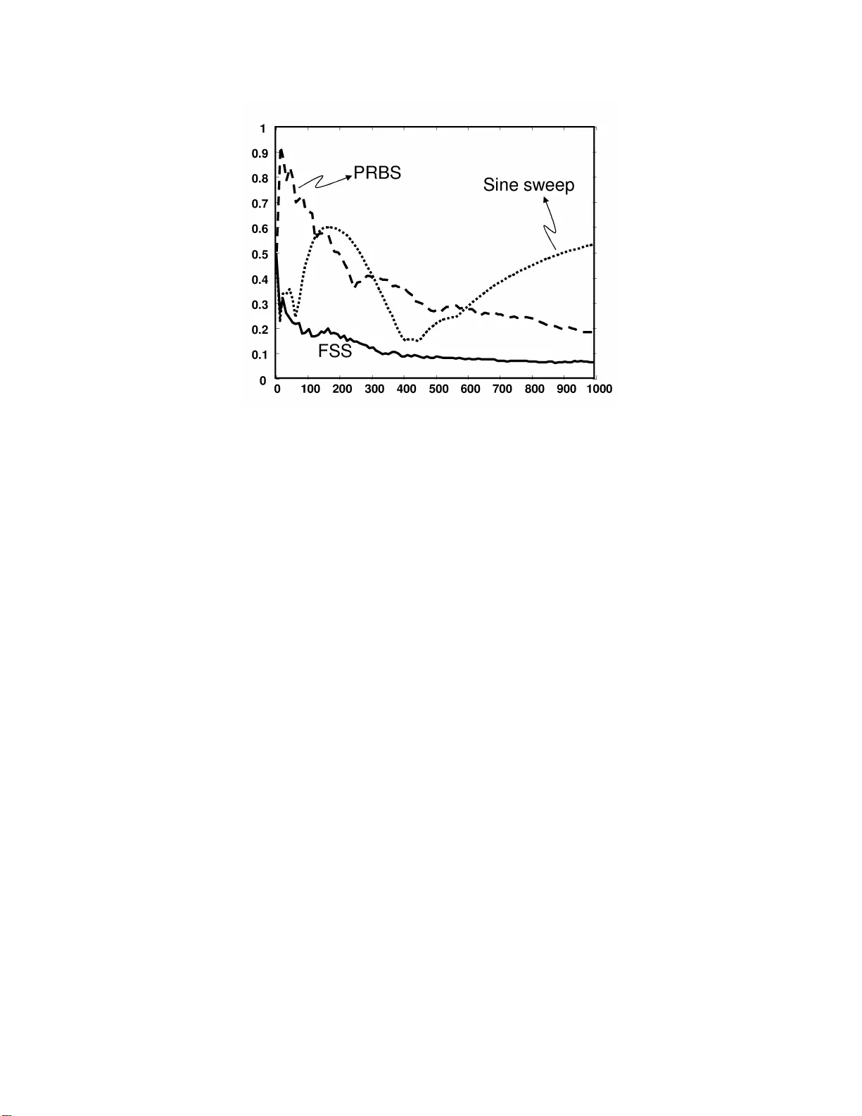
Deterministic Designs with Deterministic Guaran tees: T o eplitz Compressed Sensing Matrices, Sequence Design and System Iden tification ∗ V enk atesh Saligrama Departmen t of Electrical a nd Computer Engineering Boston Univ ersit y , Boston MA 02215 E-mail: srv@bu.edu. Abstract In this pap er we present a new family of discr e te sequences having “random lik e” uniformly decaying auto-cor relation prop er ties. The new class of infinite length sequences are higher order chirps construc ted using ir r ational num be r s. Exploiting results fro m the theory of contin ued fractions and dio phantine a pproximations, w e show that the cla s s of sequences so formed has the pro p e rty that the worst-case auto-cor relation co efficients for every finite length sequence decays at a p olyno mial r a te. These sequences display doppler immunit y a s well. W e also s how that T o eplitz m atrices fo rmed from such sequences satisfy restr icted-isometry- pr op erty ( RIP ), a concept that has play ed a central role recently in Co mpressed Sensing applica tio ns. Compressed sensing has conv ent ionally dealt with sensing matrices with arbitrar y compo nent s. Nevertheless, such arbitrary sensing matrices a re not appr o priate for linear system identifi cation and one must employ T oeplitz str uc tur ed sensing matrice s . Linear sys tem identification plays a central role in a wide v ar iety of applicatio ns such as channel estimation for multipath wir eless systems as well as control system a pplications. T oeplitz matrices ar e also des irable on account o f their filtering structure, whic h a llows for fast implement a tion together with reduced stor age require ments. ∗ This researc h w as supported b y ONR Y oung Investig ator Aw ard N00 014-02-100362 and a Presiden t ial Early Career Awa rd (PECASE), NSF CAR EER aw ard ECS 0449194, and NS F Grant CCF 0430983 and CNS- 0435353 1 1 In tro duction Sequences with sp ecial prop erties are requir ed in a num b er of applicatio n s r anging f rom comm u ni- cation systems, radar systems and sys tem iden tification. Many of these applications require families of sequences with lo w auto-correlatio n, cross-correlation and resiliency to doppler offsets. In com- m un ication systems signature sequences with lo w auto-correlation prop erties ha ve b een emplo yed in wireless co m mm u nications (see [14] ) to o v ercome self in terference due to m ulti-path effects and co-c hannel in terference due to m ulti-access comm un ications r esp ectiv ely . T o eplitz structur ed matrices naturally arise in linear system iden tification, a problem that is at the core of man y applicatio n s ranging from channel estimation in m ultipath w ireless systems to mo del estimation in con trol applications. In wireless systems the channel co efficien ts are sp arse and c hann el estimation is identic al to compr essed sensing with T o eplitz structured matrices. In parallel in sev eral con trol applications, signals with lo w auto-correlation s equences are required when a mo del parametrization is generally unkn o wn and m o dels of increasing complexit y are adap- tiv ely c hosen [16] to c haracterize the system. This usually r equires a p ersistently exciting input of arbitrary order. In add ition, an in put probing signal that is “optimal” to an y m o del order is prefer- able and this leads u s to seek ap erio dic inpu t sequences with go o d non-circular auto correlation prop erties. It can also arise in the con text of system identifica tion in the presence of u nmo d eled dynamics and noise. There is a wide array of literature dealing with system ident ifi cation in the presence of unmo d eled dynamics (see for example [13] and references therein). The solution to this p roblem requir es designing inputs that can sup p ress the corruption du e to b oth n oise and unmo d eled errors [20]. While n oise can b e ov ercome b y applying a p ersisten t input, to su p press the effect of un m o deled dynamics requires ap erio dic inpu t sequences wh ose non-circular (or zero- padded) auto correlation uniformly decreases to zero. It turns out [18, 20] that th e cont r ibution from the un mo deled dyn amics in the p arametric error is directly related to the rate of deca y of the w orst-case non-circular autocorr elation co efficien ts. In many applications su c h as multipath wireless systems [3] as well as other mediums su c h as acoustic/RF the system can b e mo deled as a finite impulse resp onse (FIR) sequence. It turns out that in these cases the su p p ort of FIR [3] is sparse. Consequen tly , this leads to the p roblem of reconstruction of sp arse FIR systems. Sparse r econstru ction has b een extensively dealt with in the con text of Comp ressed S ensing 2 (CS) [5–7, 9]. CS in volv es reco v ering a sparse signal x from linear observ ations of the form y = U x . Supp ose the true signal, x , has fewer than k non-zero comp onen ts the solution to the ℓ 0 problem reco v ers this solution if and only if ev ery sub-matrix of U formed by choosing 2 k arbitrary columns of U has full column rank. Unfortunately , it tu r ns out that the general solution is intracta b le. In [5–7, 9, 1 9] it is sh o wn that for sufficientl y small k , the ℓ 1 problem is equiv alen t to solving the ℓ 0 problem whenev er the sensing matrix U satisfies the s o calle d RIP prop erty . The R I P prop er ty of sparsit y k amoun ts to the requ iremen t that the singu lar v alues of ev ery s ub-matrix formed by selecting k columns of U is close to one. T he question no w arises as to what matrice s satisfy RIP prop erty . Earlier wo r k on C S established RIP prop ert y for random constructions and recen t wo r k has p ro du ced deterministic designs b ased on deterministic sequence constructions [8, 11]. Nev ertheless, this setup is not d ir ectly applicable to the sparse FIR sys tem iden tification p rob- lem. Sp ecifically , in this setting the output is the conv olution of in puts w ith th e channel co efficient s . This amoun ts to taking a pro du ct of T o eplitz matrix of the inputs and a v ector consisting of FIR co efficien ts as comp onents. Th er efore, this calls for RIP p rop erty for T o eplitz matrices. Motiv ated b y these issu es [1] consider random T o eplitz matrices and d eriv e in formation theoretic limits while [3, 4] d ev elop RIP p rop erties for random generated T o eplitz m atrices. In this pap er we design deterministic T o eplitz matrices having guarante ed RIP prop erties. T o accoun t for compressed sensing in the con text of sys tem identi fication we fi rst present a new family of discrete sequences ha vin g “random lik e” uniformly deca ying auto-correla tion p rop erties. The new class of infin ite length sequ en ces are higher order c hirps constru cted u s ing irrational n u m b ers. Exploiting results from the theory of cont inued fr actions and diophan tine app ro ximations, w e show that the class of sequ en ces s o formed has the prop ert y that the w orst-case auto-correlation co efficien ts f or ev ery fin ite length sequence deca ys at a p olynomial rate. W e also sho w that T o eplitz matrices formed from suc h sequen ces satisfy restricted-isometry-prop ert y (RIP). Linear system iden tification pla ys a cen tral role in a w ide v ariet y of applications such as channel estimation for multipath w ireless systems as w ell as con trol system applications. T o eplitz matrices are also desirable on accoun t of their filtering structur e, whic h allo ws for fast implementa tion together w ith reduced storage requiremen ts. Additionally , w e show that th ese sequences are imm un e to doppler offsets. The organization of the pap er is as follo ws. In S ection 2 we motiv ate T oeplitz structur ed 3 matrices in CS and System Identi fication. W e th en form u late the problem of CS in terms of seeking sequences with auto correlation prop erties. This m otiv ates th e design of sequences wh ic h is dealt with in Section 3. The follo wing Section 4 deals with matrix constructions th at fur ther impro ve up on the RIP prop erties. W e finally conclude with a br ief discussion of pr actical and implemen tational issues. 2 Problem Setup Linear sys tem iden tification pr oblems are generally c haracterized by measured output, y , the inpu t, u , Gaussian n oise, w , and a linear time-in v arian t system, G that are related b y the f ollo wing discrete time equati on. y ( t ) = Gu ( t ) + w ( t ) , t = 0 , 1 , . . . , n , (1) where, the system G is ident ifi ed b y its k ernel, { g t } , w hic h is usually assum ed to b e an element of ℓ 1 , w here, ℓ 1 is identified with the sp ace of b oun ded analytic functions on th e unit disc [20]. The ob jectiv e is to estimate G in some metric norm. Obvi ou s ly , with fi n ite data arbitrary elemen ts of ℓ 1 cannot b e estimated. One typica lly assumes in this conte xt that the s ystem can b e d ecomp osed in to a finite dimensional mo del, H and a small residual unmo d eled d ynamics, ∆. If the fin ite parametrization happ en s to b e the class of fi nite impulse resp onse s equences (FIR) of ord er m we obtain in expanded notati on, y s = Gu s + w s = FIR Model z }| { m X k =0 g k u s − k + Residual Error z }| { s X k = m +1 g k u s − k + w s (2) The task is to estimate H ≡ { g 0 , g 1 , . . . , g m } giv en that ∆ ≡ ( g m +1 , g m +2 , . . . . ) has ℓ 1 norm smaller than γ . F urther expanding into matrix notation w e get,         y 1 y 2 . . . y n         =         u 0 0 . . . . . . u 1 u 0 0 . . . . . . . . . . . . . . . u n − 1 u n − 2 . . . u 0                 g 1 g 2 . . . g n         +         w 1 w 2 . . . w n         (3) No w in the absence of noise it is clear that a pulse input of unit-amplitude is su fficien t to reco v er the FIR mo del exactly . On th e other hand p ersisten t noise can only b e a ve r aged out by a p ersistent 4 input. Ho w ever, a p ersisten t input will also ”excite” th e unmo deled error. In particular for the ab o ve equ ation, w henev er, s ≥ m + 1, the data also cont ains con trib utions from the unmo deled dynamics. F or a p erio dic input , u , with u s + l = u s , the data for s = 0 , l , 2 l, . . . can b e w ritten as: y s = s X k =0 g k u s − k + w s = ( g 0 + g 1 + . . . ) u 0 + ( g 1 + g l +1 + . . . ) u 1 + . . . + w s Th us one obtai n s information only on linear combinatio n s of the g k ’s and not the individual co ef- ficien ts. It is therefore imp ossible to determine only the model-co efficien ts no matter ho w long the input signal and ho w large the length of the p erio d. Therefore, no matter ho w large th e p erio d, in the w orst case the un mo deled error will couple with the mo del-set dynamics. Although w e describ e the simple case of FIR mo dels and residu al err or, similar d ecomp ositions can b e obtained for more general p arameterizatio n s [18, 20]. W e define ap erio dic auto correlations function to c h aracterize the design problem for robus t iden tification. Definition 1. A n-window ap erio dic auto correlation f u nction (ACF) of a real/complex v alued sequence, { u t } t ∈ Z + , is defined as: ˜ r n u ( τ ) = 1 n n − τ X s =0 u s u ∗ s + τ , τ ∈ Z where the asterisk denotes the complex conjugate. It tur ns out th at a sufficien t cond ition (see [18] for necessary condition) on inp ut sequences f or estimation of the optimal fi nitely parameterize d mo del is that the worst-case ap erio dic autocorre- lation asymptotica lly app roac h zero. max 0 <τ ≤ n | ˜ r n u ( τ ) | | ˜ r n u (0) | − → 0 The sp ecial case when the un mo deled dynamics, ∆, is negligible is of imp ortance in many applications. Here the impulse resp onse terminates after p co efficien ts and an inp ut of length n is usually applied. Consequently , w e get y s = s X k =0 g k u s − k + w s , s ≤ p and y s = p X k =0 g k u s − k + w s , s > p 5 This corresp onds to a “fat” T o eplitz matrix of the form: U =                   u 0 u 1 . . . . . . . . . u 0 u 1 u n − 1 . . . . . . u n − 1                   . (4) where the n u m b er of columns in the ab ov e matrix is p . There is an other situation that arises in th e FIR context when th e output resp ons e is observ ed in s teady state. Here, the input u t is assu m ed to start f r om time t = − ∞ and th e output is obs erv ed b et ween time t = p un til t = p + n − 1. In this situation w e get , y s = p X k =0 g k u s − k + w s Organizing the ab ov e equatio n as a matrix for s ≥ p leads to the follo wing T o eplitz matrix: U =         u p u p − 1 . . . u 2 u 1 u p +1 u p . . . u 3 u 2 . . . . . . . . . . . . . . . u p + n − 1 u n + k − 2 . . . . . . . u n         , (5) Note that the structure of th e steady state matrix leads to time-dep enden t auto-correlations, w hic h w e define b elo w: Definition 2. An n-window auto correlation fu nction (ACF) of a real/complex v alued sequence, { u t } t ∈ Z + , is defined as: r n u ( t, τ ) = 1 n t + n X s = t u s u ∗ s + τ , τ ∈ Z where the asterisk denotes the complex conjugate. So far the discussion ab o ve h as fo cused on different asp ects of sy s tem identificat ion. W e will no w relate this to compressed s ensing p roblems. These problems arise when the sup p ort of FIR co efficien ts is sparse. As w e describ ed in the previous section a central ingredient t ypically emp loy ed 6 in establishing that conv ex programming algorithms lead to sparse reco v ery is the so called restricted isometry prop ert y (RIP). W e describ e the RIP prop ert y next. W e follo w closely the d ev elopment in [2]. Let D b e the diagonal m atrix consisting of ℓ 2 norms of eac h column of U . Let, I q b e the collect ion of all su bsets of { 1 , 2 , . . . , p } of cardinalit y q . Enumerate th e elemen ts of this sub - collect ion as l = 1 , 2 , . . . ,  n q  and let π ( l ) denote the lth elemen t of I q . U π ( l ) , D π ( l ) denote the sub-matrices of U, D resp ectiv ely obtained by selecting columns with indices in π ( l ). Let, Σ l b e the n ormalized correlation matrix, i.e ., Σ l = D − 1 / 2 π ( l ) U T π ( l ) U π ( l ) D − 1 / 2 π ( l ) W e next defin e the RIP p rop erty . Definition 3. [RIP prop ert y] A n × p sensin g matrix, U , c haracterized b y th e trip le ( n , p, q ) is said to ha v e RIP prop ert y of order q if there is a num b er δ q ∈ [0 , 1) suc h that ev ery correlation matrix Σ l satisfies: (1 − δ q ) ≤ λ min (Σ l ) ≤ λ max (Σ l ) ≤ (1 + δ q ) , ∀ l = 1 , 2 , . . . ,  n q  Note that RIP p rop erty of order q immediately implies RIP pr op ert y of smaller order. This follo ws from th e observ at ion [2] that for ˜ π ( l ) ⊂ π ( l ) w e get λ min ( U T π ( l ) U π ( l ) ) ≤ λ min ( U T ˜ π ( l ) U ˜ π ( l ) ) , λ max ( U T ˜ π ( l ) U ˜ π ( l ) ) ≤ λ max ( U T π ( l ) U π ( l ) ) W e are no w left to establish eigen v alue b ounds for the correlati on matrices of all orders. First note that the co efficients of the correlatio n matrix are the auto correlation co efficien ts. As remarked earlier the auto correlation co efficients are d ifferent for th e differen t matrices. In particular for Equation 5 w e ha ve, Σ l =  r n u ( t, s − t ) r n u ( t, 0)  t,s ; t, s ∈ π ( l ) ∈ I q On the other hand for Equation 4 we get Σ l =  ˜ r n u ( t − s ) ˜ r n u (0)  t,s ; t, s ∈ π ( l ) ∈ I q W e can no w state a s u fficien t condition for RIP p rop erty based on eigen v alue b ound s for cor- relation matrices of [10]. Th ese b ounds are based on a straight forw ard application of Gersgorin theorem. T he reader is also referred to Theorem 2 of [3] for a closely r elated result deriv ed for random T o eplitz matrix constructions. 7 Theorem 1. S upp ose U is T oeplitz matrix of Equation 5.Then U satisfies the RIP prop ert y of order q if R = max π ( l ) ∈ I q X t,s ∈ π ( l ) , s 6 = t | r n u ( t, s − t ) | | r n u ( t, 0) | < 1 No w supp ose U is a T o ep litz matrix as in Equation 4. Then U satisfies the RIP p rop erty of ord er q if R = m ax I q X τ ∈ I q | ˜ r n u ( τ ) | | ˜ r n u (0) | < 1 Pro of. T h e p ro of follo ws b y a str aightforw ard application of Gershgorin’s th eorem app lied to Correlation matrices (see P age 60 in [10]). In particular f rom [10] it follo ws th at the eigen v alues of the correlation matrix Σ l can b e upp er and lo w er b ound ed b y the sum of the off-diagonals. In other w ords, if R l = X t,s ∈ π ( l ) , s 6 = t | r n u ( t, s − t ) | | r n u ( t, 0) | then, λ min (Σ l ) ≥ 1 − R l , λ max (Σ l ) ≤ 1 + R l No w to ensure ev ery correlation matrix satisfies the RIP prop ert y w e tak e the maxim u m o ve r all the elemen ts in I q . The condition for Equation 4 follo ws in an identic al fashion an d is omitt ed . Our fir st attempt at establishing RI P pr op erty will b e b y quant if y in g th e worst-ca se autocorre- lation co efficien t. In particular in Section 3 we will describ e sequences whose w orst-case auto corre- lation co efficients d eca y at a p olynomial rate. In the follo wing Section 4 we will directly deal with matrix constructions. Definition 4. A b ound ed sequence, { u ( t ) } , t = 1 , 2 , . . . , n + p − 1, is said to ha ve a uniformly p olynomial deca y (PD ACF) p rop erty if there is a γ > 0 suc h th at the w ors t-case auto correlation satisfies:     r n u ( t, τ ) r n u ( t, 0)     ≤ C n − γ , ∀ t = 1 , 2 , . . . , p, 0 ≤ t + τ ≤ p Corollary 1. The T o eplitz matrix A of Equation 5 RIP pr op erty of or der q = O ( n γ ) if the se quenc e satisfies PDACF pr op erty with de c ay c o efficient γ . Note that the PD ACF pr op ert y may not h old for arbitrary n um b er of columns n and w e m ake this p recise lat er. 8 Figure 1: Comparison of W orst-case auto-correlati on functions for v arious lengths of a 2 15 − 1 order PRBS, s in e-sw eeps and Higher-order-c hirps or fast sine sw eeps (FSS). In summary a simple means to realize RIP prop ert y is to obtain c h aracterizatio n s with lo w au- to correlation. It can b e argued th at f or all pr actical purp oses one could p ossibly take truncations of pseudo-random binary sequences (PRBS) sequences with arbitrary long p erio d. Ho we ver, it turns out that tru ncations of PRBS sequences do n ot necessarily ha ve small auto correlations. Un f ortu- nately the auto correlation expr essions in Theorem 1 inv olv es correlations of truncated sequences. In Figure 1 the wo r st-case auto-correlatio n s of tru ncated PR BS of p erio d 2 15 − 1 has b een plotted. As seen such truncated sequences can ha ve p o or autocorrelations. Finally , it is p erhaps su rprising that the widely used sine-sweep, u ( t ) = exp ( iαt 2 ) , α ∈ I R , t = 0 , 1 , 2 , . . . , do es not meet the requirement s either. In [20], w e sho w that, lim sup max 0 <τ ≤ n | ˜ r n u ( τ ) | ≥ 1 / 2 The b asic reason is that the auto-correlati on fu nction turn s out to b e equal to sin( nτ α/ 2) / ( n sin ( τ α )) and subsequ en ces τ j , and n j can b e suitably c hosen so th at the limiting v alue of τ j α mod (2 π ) tends to zero W e n ext p r o vide su fficien t conditions in terms of worst-c ase deca y of auto correlation co efficien ts. 9 Definition 5. A b ounded sequence, { u ( t ) } , t = 1 , 2 , . . . , n , is said to hav e an ap erio d ic uni- formly polynomial deca y (PD ACF) prop erty if there is a γ > 0 suc h that the worst-ca se ap erio dic auto correlation satisfies:     ˜ r n u ( τ ) ˜ r n u (0)     ≤ C n − γ , ∀ τ = 1 , 2 , . . . , n Corollary 2. The T o eplitz matrix A of E quation 4 has an RIP pr op erty of or der q = O ( n γ ) if the se quenc e satisfies PDACF pr op erty with de c a y c o efficient γ . Note that the PD ACF pr op ert y may not h old for arbitrary n um b er of columns n and w e m ake this p recise lat er. 3 Sequence Design It turn s out that higher-order-chirps (HOC) sequences are PDA CF sequen ces. These are determin- istic sequ ences of the form u ( t ) = exp( i 2 π αt 3 ) where α is some ir rational num b er. In app lications the real part of the complex sequ en ce w ill actually b e app lied and to simplify our exp osition we consider the complex v alued signal here. Theorem 2. The third order c hirp sequences has the PD ACF pr op ert y for th e ACF function as defined in Definition 4 with γ = 0 . 25 for τ ≤ λn for all quadratic irrational n umb ers. Remark: Recall that algebraic n umb ers are those num b ers th at are ro ots of an y p olynomial defined o v er a field of in tegers. Remark: Note that the higher-order c hirps are complex v alued. Ho w ev er, iden tical prop erties hold for real-part and imaginary part of these signals. The p ro of is br ok en do wn into several steps. In the fi rst step we will upp er b oun d the ACF function b y means of simpler fu nctions. Denote b y k x k the distance of x from the close s t in teger: k x k = m in A ∈ Z | x − A | (6) and [ x ] = argmin A ∈ Z | x − A | The follo wing elemen tary facts f ollo w s: 10 Prop osition 1. Th e follo win g hold: k k x k = k k k x kk | sin(2 π x ) | ∈  k x k 2 , k x k  Pro of. T o prov e the first assertion we note that: [ x + k ] = [ x ] + k , ∀ k ∈ Z + Next we p r o ceed as follo ws: k k x k = | kx − [ k x ] | = | kx − [ k x − k [ x ] + k [ x ]] | = | k x − [ k ( x − [ x ])] − k [ x ] | = | k ( x − [ x ]) − [ k ( x − [ x ])] | T o obtain b ounds for the sin usoid function, we observe that: | sin(2 π x ) | = | s in (2 π k x k ) | ∈ [0 . 5 k x k , k x k ] where the last assertion is a standard result in elementa r y calculus. With these preliminaries we can redu ce the expression for ACF in terms of the f unction k · k as in th e follo wing lemma. Lemma 1. The A CF function, | r n u ( τ ) | , τ ∈ Z + , for the HOC s atisfies the follo wing inequalit y for an y irrational n umber α ∈ I R. | r n u ( t, τ ) | 2 ≤ 1 n p X k =0 3 1 + n k k τ α k , 1 ≤ τ ≤ p = λn and for the aperio d ic A CF | ˜ r n u ( τ ) | 2 ≤ 3 n n X k =0 1 1 + n k k τ α k , 1 ≤ τ ≤ n (7) Pro of. First, the A CF function and its ap erio dic counte r part can b e s im p lified by straightforw ard algebraic manipulations as follo ws: | ˜ r n u ( τ ) | 2 ≤ 1 n 2 n − τ X k =1     sin(2 παk τ ( n − τ )) sin(2 παk τ )     + C n = C n + 1 n 2 L X k =1     sin(2 π Lk x ) sin(2 π k x )     , L = n − τ , x = τ α, 1 ≤ k , τ ≤ n 11 Similarly , | r n u ( t, τ ) | 2 ≤ 1 n 2 n X k =1     sin(2 π αk τ n ) sin(2 π αk τ )     + C n = C n + 1 n 2 n X k =1     sin(2 π nk x ) sin(2 πk x )     , x = τ α, 1 ≤ k , τ ≤ p = λn T o further simp lify these expressions w e consider the function, H L ( · ): H L ( x ) = 3 L 1 + L k x k and obtai n the follo win g p rop erty . Prop osition 2. T he f u nction H L ( x ) is a monotonic function ov er L , i.e., H j ( x ) ≤ H k ( x ) f or j < k . F urthermore, it satisfies:     sin(2 πL x ) sin(2 πx )     ≤ H L ( x ) Pro of. Con s ider the function, H L ( · ): H L ( x ) = 3 L 1 + L k x k (8) Since, | sin(2 π Lx ) / sin (2 π x ) | ≤ L , it follo w s     (1 + L k x k ) sin (2 π Lx ) sin(2 π x )     ≤ L + L k x k | sin(2 π x ) | | sin(2 π Lx ) | ≤ 3 L where for last inequalit y w e ha ve used Prop osition 1 Next, we sho w that H L ( · ) is monotonic in L . Su pp ose, we ha ve giv en t wo in tegers, n, m , with n < m , it follo w s that: m + mn k x k ≤ n + mn k x k ⇐ ⇒ m 1 + m k x k ≤ n 1 + n k x k The result no w follo ws by insp ection. Note that th e up p er b ound s for b oth cases are iden tical for λ = 1, i.e., p = n . F or simplicit y w e consider λ = 1 case and commen t on what hap p ens when λ > 1 la ter. The main difficu lty now in establishing the resu lt is th at lim inf q k q α k = 0 for ev ery real n u m b er, i.e., k j α k comes close to zero infi nitely often. T he pro of therefore rests on the fact that v ery few terms in the s equ ence ( k τ α k , k 2 τ α k , . . . , k nτ α k are close to zero for any ph ase 0 < τ ≤ n . A w ell kno w n result in con tinued fraction expansion theory [12] pro vid es h ow closely can rational n u m b ers app ro ximate irrational num b ers: 12 Theorem 3. If α is a quadratic irrational num b er(i.e. irrational solution of a quadr atic p olynomial) there exists a constan t C α > 0 suc h that, C α j ≤ k j α k , j ∈ Z + F urthermore, for ev ery constan t ǫ > 0, f or almost all irrational num b ers α ∈ (0 , 1) except on set of leb esgue measure zero, the inequalit y , k q α k < 1 q log 1+ ǫ q , q ∈ Z + has only a finite num b er of solutions. Remark: T o put things in to p ersp ectiv e w e p oin t out that C α = 1 √ 5 for the golden ratio, α = (1 + √ 5) / 2. Unfortunately , this inequalit y alone is insufficien t for derivin g the upp er b ounds f or w orst-case A CF, as sho wn b elo w: max 0 <τ ≤ n 1 n n X k =0 1 1 + n k k τ α k ≤ 1 n n X k =1 1 1 + nC α k n 6− → 0 Consequent ly , we n eed to rely on more in tricate prop erties of con tin u ed fractio n theory to dev elop an accurate estimate. The abov e setup suggests that it is con v en ient to deal w ith th e family of n irrational num b ers, τ α with 0 < τ ≤ n . W e denote b y the sym b ol β an y irrational n u m b er in this family . S p ecifically , w e let β ∈ S ( α, n ) = {k τ α ) k ; τ = 1 , 2 , . . . , n } Note that by employing Prop osition 1 w e can f urther simplify the expression in Equation 7 as follo ws: 1 n n X k =1 1 1 + n k k τ α k = 1 n n X k =1 1 1 + n k k ( k β k ) k , for some β ∈ S ( α, n ) Consequent ly , we need to show that: 1 n n X k =0 1 1 + n k k β k ! 1 / 2 ≤ n − γ , ∀ β ∈ S ( α, n ) W e summarize prop er ties from elementa r y con tinued fraction theory for the purp ose of completion next. Th ese pr op erties and the acc ompan yin g n otation ha v e b een adopted from [17]. 13 Con tinued F ractions: The con tinuous fr action expansion of any p ositiv e irrational num b er β is giv en b y: β = [ a 0 ; a 1 , a 2 , . . . , a j , . . . ] = a 0 + 1 a 1 + 1 a 2 + 1 ...a j ... , a j ∈ Z + where for the sake of brevit y the first expr ession is typicall y used to denote the expan s ion. In our con text w e hav e β < 1 / 2 and so a 0 = 0. By truncating the con tinuous f raction expansion w e obtain a sequence of rational num b ers called con v ergents, i.e., A k B k = [ a 0 ; a 1 , a 2 , . . . , a k ] The n umerator and denominator of the con vergen ts satisfy the follo win g r ecur sion: A k +1 = a k +1 A k + A k − 1 , A − 1 = 1; A 0 = a 0 , k ≥ 0 (9) B k +1 = a k +1 B k + B k − 1 , B − 1 = 0; B 0 = 1 , k ≥ 0 (10) Since, a k s are p ositiv e in tegers the n u merator and denominator sequences B k , A k s form a strictly monotonically increasing sequence. It follo ws that: B k = a k B k − 1 + B k − 2 = ( a k a k − 1 + 1) B k − 2 + B k − 3 ≥ 2 B k − 2 ≥ 2 ( k − 1) / 2 (11) where the last equation follo w s from the fact that a k ≥ 1. Optimal Appro ximation: The con vergen ts are optimal rational appro ximants, in that, the kth con ve r gen t is the b est appro ximation to the irrational num b er among all rationals wh ic h hav e a smaller denominator: k B k β k ≤ k j β k , ∀ 0 < j ≤ B k , k ≥ 1 (12) F or con v enience we denote b y , D k = B k β − A k The D k s f ollo w s a simp le a recursion iden tical to Equ ations 9, i.e., D k = a k D k − 1 + D k − 2 , D − 1 = − 1 (13) It follo ws that th e so called ev en con vergen ts, A 2 k /B 2 k , m on otonically approac h β from th e righ t while the o dd con vergen ts, A 2 k + 1 /B 2 k + 1 , approac h β from the left as sho w n in Figure 2. It turn s 14 Figure 2: I llu stration of ho w ev en and odd con verge n ts app roac h an ir rational n umb er α out that the v alue of D k is b ounded from ab o v e and b elo w b y the size of the denominators giv en b y: 1 2 B k +1 ≤ 1 B k + B k +1 ≤ | D k | ≤ 1 B k (14) Ostro w ski Decomp osition: In the so called Ostr o wski’s repr esen tation, eac h integer, m , is expressed as a linea r com b ination of th e B k s. It turn s out th at this repr esen tation is unique in the follo wing sense. An y in teger m ∈ Z + with B p ≤ m ≤ B p +1 can b e u niquely decomp osed as: m = p X j =0 c j +1 B j (15) with 0 ≤ c j +1 ≤ a j +1 for j ≥ 1 and 0 ≤ c 1 < a 1 . Moreo ve r, c j = 0 if c j +1 = a k +1 . This decomp osition is obtained by fir s t dividing m with the largest d enominator, B p , smaller th an m and then decomp osing the remainder with a corresp onding large st denominator and so on. Lo wer Bounds to Rational Appro ximation: The s ignifi cance of Ostrowski representa tion follo ws from u pp er and lo w er b ounds. First note that due to translation in v ariance w e ha ve , k mβ k = k p X j =0 c j +1 B j β k = k p X j =0 c j +1 B j β − p X j =0 c j +1 A j k = k p X j =0 c j +1 D j k The follo wing Lemma from [17] (Lemma 1 Ch ap. 2) will b e useful: Lemma 2. | p X j =0 c j +1 D j | ≥ | ( c γ ( m )+1 − 1) D γ ( m ) | + | D γ ( m )+1 | T o derive b ound s we need to d efine the t yp e of an in teger m . Let, m = P p j =0 c j +1 B j , b e the Ostro wsk i representati on for m . The type γ ( m ) of an int eger m is an in teger defined as: γ ( m ) = min { j | c j +1 6 = 0 } 15 W e also defin e γ ∗ n to b e the maxim u m p ossible type in Z n = { 1 , 2 , . . . , n } , i.e., γ ∗ n = m ax { γ ( m ) | m = 1 , . . . , n } Prop osition 3. Th e maximum t yp e, γ ∗ n , in the set Z n is smaller than 2 log 2 (2 n ). Pro of. If m ∈ Z n is of t yp e γ ( m ), then, from the ostro wski decomp osition it follo ws th at m ≥ B γ ( m ) ≥ 2 γ ( m ) − 1 2 = ⇒ 2 log 2 m + 1 ≥ γ ( m ) where, we ha ve used Equation 11 f or the second in equ alit y . Thus, the largest p ossible t yp e in Z n is λ n = 2 log 2 n . Since, t yp e is a p ositiv e intege r ranging from 0 to 2 log 2 n , the result follo ws b y insp ection. The t yp e of the in teger, q , signifies how small k qβ k can get. W e ha v e the follo win g result from [17] (Theorem 1 Chap. 2) that pr ecisely charact erizes this connection: Theorem 4. Let 0 < β < 1 / 2 and the in teger, m , hav e t yp e γ ( m ) ≥ 1. Then, k mβ k = | p X j =0 c j +1 D j | The ab o ve results lead to the follo wing pr ecise c haracterizatio n of ho w typ e is asso ciated with k mβ k : Lemma 3. L et 0 < β < 1 / 2 b e an irr ationa l numb er and m > 1 a p ositive inte ger. Then, k mβ k ≥                                    min (( c 1 − 1) | D 0 | + ( a 2 − c 2 ) | D 1 | , ( a 1 − c 1 ) | D 0 | + c 2 | D 1 | ) ≥ m in  c 1 − 1 2 B 1 + a 2 − c 2 2 B 2 , a 1 − c 1 2 B 1 + c 2 2 B 2  γ ( m ) = 0 c γ ( m )+1 − 1 2 B γ ( m )+1 + a γ ( m )+2 − c γ ( m )+2 2 B γ ( m )+2 γ ∗ n − 1 ≥ γ ( m ) ≥ 1 c γ ∗ n +1 k B γ ∗ n β k γ ( m ) = γ ∗ n ≥ 1 16 Pro of. Th e case of γ ( m ) = γ ∗ n is a d irect consequence of Theorem 4. T o establish the s econd case w e p ro ceed b y noting that for γ ( m ) ≥ 1 w e h a ve k mβ k = | P p j =0 c j +1 D j | and from the fact that the ev en and o dd D ′ k s ha v e opp osite sign we get: | p X j =0 c j +1 D j | = | c γ ( m )+1 D γ ( m ) + c γ ( m )+2 D γ ( m )+1 + c γ ( m )+3 D γ ( m )+2 + . . . + c γ ( m )+2 j D γ ( m )+2 j − 1 + c γ ( m )+2 j +1 D γ ( m )+2 j + . . . | ≥ | c γ ( m )+1 D γ ( m ) + c γ ( m )+2 D γ ( m )+1 + a γ ( m )+4 D γ ( m )+3 + a γ ( m )+6 D γ ( m )+5 + . . . | ≥ | c γ ( m )+1 D γ ( m ) + a γ ( m )+2 D γ ( m )+1 + ( c γ ( m )+2 − a γ ( m )+2 ) D γ ( m )+1 + a γ ( m )+4 D γ ( m )+3 + a γ ( m )+6 D γ ( m )+5 + . . . | The second inequalit y follo ws from th e fact that w e hav e remo v ed all the terms with the same sign as D γ ( m ) (i.e. terms of the form D γ ( m )+2 j ) while taking the maxim um p ossible v alues for terms of opp osite sign. The third inequalit y is just a restatemen t of the third term. Next w e utilize Equation 13 to mak e the su bstitution th at D k − D k − 2 = a k D k − 1 and ge t, | p X j =0 c j +1 D j | ≥ | c γ ( m )+1 D γ ( m ) + ( c γ ( m )+2 − a γ ( m )+2 ) D γ ( m )+1 + a γ ( m )+2 D γ ( m )+1 + a γ ( m )+4 D γ ( m )+3 + a γ ( m )+6 D γ ( m )+5 + . . . | ≥ | c γ ( m )+1 D γ ( m ) + ( c γ ( m )+2 − a γ ( m )+2 ) D γ ( m )+1 +( D γ ( m )+2 − D γ ( m ) ) + ( D γ ( m )+4 − D γ ( m )+2 ) + . . . | ≥ | ( c γ ( m )+1 − 1) D γ ( m ) + ( c γ ( m )+2 − a γ ( m )+2 ) D γ ( m )+1 | Finally , we kn o w from Equ ation 14 that | D γ ( m ) | ≥ 1 B γ ( m ) + B γ ( m )+1 ≥ 1 2 B γ ( m )+1 Next obs erving that D γ ( m ) and D γ ( m )+1 are of opp osite signs the result follo ws. Finally , to establish th e first case, i.e., γ ( m ) = 0 w e note that a lo wer b ound f or | P p j =0 c j +1 D j | follo ws ident ically as the case for γ ( m ) ≥ 1. W e next derive an u p p er b ound by excludin g all term s of opp osite sign (except for the term con taining D 1 ) as D 0 and include the maximum p ossible terms of the same sign. Through algebraic manipulations as for the low er b ound and noting that th e ev en D ′ k s are of the same sign we get: | γ ∗ n X j =1 c j +1 D j | ≤ | c 1 D 0 + c 2 D 1 + a 3 D 2 + a 5 D 4 + . . . | ≤ | c 1 D 0 + ( c 2 − 1) D 1 | 17 Next, su bstituting Equation 13 for D 1 = a 1 D 0 − 1 w e get: | γ ∗ n X j =1 c j +1 D j | ≤ | 1 + ( c 1 − a 1 ) D 0 + c 2 D 1 | No w it follo ws that the latter term is strictly less than 1 by noting th at D 0 = β > 0 and D 1 is negativ e and: | 1 + ( c 1 − a 1 ) D 0 + c 2 D 1 | ≤ | 1 + (( a 1 − 1) − a 1 ) D 0 | ≤ | 1 − D 0 | ≤ 1 W e also n ote that D 2 = a 2 D 1 + D 0 > 0, and s o, 1 + ( c 1 − a 1 ) D 0 + c 2 D 1 = c 1 D 0 + ( c 2 − 1) D 1 ≥ c 1 D 0 + ( a 2 − 1) D 1 ≥ ( c 1 − 1) D 0 − D 1 + D 2 > 0. Thus w e ha ve a u pp er and lo wer b ound for | P γ ∗ n j =1 c j +1 D j | that are b oth p ositiv e and smaller than 1, i.e., 0 < ( c 1 − 1) D 0 + ( c 2 − a 2 ) D 1 ≤ | γ ∗ n X j =1 c j +1 D j | ≤ 1 + ( c 1 − a 1 ) D 0 + c 2 D 1 < 1 No w noting that D 0 is p ositive and D 1 is negativ e establishes the fi rst inequalit y for γ ( m ) = 0. Also substituting the lo w er b ounds of Equation 14 it follo ws that the second inequalit y for γ ( m ) = 0 is also satisfied. T o complete the ab ov e set of results w e need a b ound for the situation wh en γ ( m ) = γ ∗ n = 0. W e ha v e the follo win g corollary: Corollary 3. L et 0 < β < 1 / 2 b e an irr ational nu mb er and m > 1 a p ositive i nte ger and γ ( m ) = γ ∗ n = 0 . Then, k mβ k ≥ min (( c 1 − 1) | D 0 | , ( a 1 − c 1 ) | D 0 | ) W e are no w ready to prov e th e main theorem by a com bination of the ab o ve well-kno wn prop- erties in con tin ued fraction theory . The main outline of the pro of is as follo ws. Lemma 3 and Corollary 3 p oin ts to the fact that th e t yp e of a num b er con tr ols the v alue of k mα k . This m otiv ates partitioning of the set Z n = { 1 , 2 , . . . , j, . . . , n } based on its t y p e and computing the con tribu tions for eac h t yp e. Th is leads us to defining the follo win g sets: A l,c = { m ∈ Z n | γ ( m ) = l , c γ ( m )+1 = c, in the Ostr o wski expansion for m } A l,c, d = { m ∈ Z n | γ ( m ) = l , c γ ( m )+1 = c, c γ ( m )+2 = d in the Ostro wski expansion for m } W e sho w in the sequel th at th e cardinalit y decreases exp onent ially with the type. 18 Lemma 4. The card in alit y of A l,c in th e set Z n is give n by: # A l,c ≤    2 j n B l +1 k l < γ ∗ n 1 l = γ ∗ n and the cardinalit y of the set, A l,c 1 ,c 2 is b ounded by the cardinalit y of the set, A l +1 ,c 2 . Pro of. Th e p ro of requires the follo wing prop osition. Prop osition 4. Giv en, t wo p ositiv e int egers, q , r and their corresp onding Ostro wsk i repr esen ta- tions, { c j ( q ) } , { c j ( r ) } , it follo ws th at: q < r ⇐ ⇒ ∃ l ∈ Z + suc h that c l ( q ) < c l ( r ); c j ( q ) ≤ c j ( r ) , ∀ j ≥ l Pro of. ( ⇐ = case) Supp ose there is an l satisfying the hyp othesis. It then follo w s that, r − q = p X j =0 c j +1 ( r ) B j − p X j =0 c j +1 ( q ) B j = l − 2 X j =0 ( c j +1 ( r ) − c j +1 ( q )) B j + p X j = l − 1 ( c j +1 ( r ) − c j +1 ( q )) B j > − l − 2 X j =0 c j +1 ( q ) B j + B l − 1 It remains to sho w that the last term is p ositiv e. W e do this by ind u ction. Clearly , the hyp othesis is tru e for l = 1. Supp ose, the induction hyp othesis is true for l = k , then for l = k + 1, w e ha v e: B k +1 = a k +1 B k + B k − 1 ≥    ( a k +1 − 1) B k + P k − 1 j =1 c j +1 B j , c k 6 = 0 a k +1 B k + P k − 2 j =1 c j +1 B j , c k = 0 where, the inequ alities follo w from ind u ction hypothesis and Equation 9. The RHS corresp onds to all th e admissible c j s and the pro of follo ws . (= ⇒ case ) This follo ws b y con tradiction and rev ersing the p revious argumen ts. Pro of. ( Lemma 4 ) Any integ er q ∈ A k ,c has an Ostrowski decomp osition: q = γ ∗ n X j = k c j +1 ( q ) B j ≡ (0 , . . . , 0 , c k +1 ( q ) , c k +2 ( q ) , . . . , c γ ∗ n +1 ( q )) , c k +1 = c 19 where c k + l s are arbitrary intege r s constrained only b y prop erty (C). Consequen tly it f ollo w s fr om Prop osition 4, for an y other in teger, p ∈ A k ,c , p > q th at, ∃ l ≥ k + 2 suc h that c l ( p ) > c l ( q ) , & c j ( p ) ≥ c j ( q ) , ∀ j ≥ l This implies that, p − q = γ ∗ n X j = k +1 ( c j ( p ) − c j ( q )) B j − 1 = γ ∗ n X j = k +2 ( c j ( p ) − c j ( q )) B j − 1 ≥ B l − 1 − l − 1 X j = k +2 c j ( q ) B j − 1 (16) ≥ a l − 1 B l − 2 − l − 1 X j = k +2 c j ( q ) B j − 1 ≥ B l − 2 − l − 2 X j = k +2 c j ( q ) B j − 1 ≥ . . . ≥ B k +2 − c k +2 B k +1 ≥ ( a k +2 − c k +2 ) B k +1 ≥ B k +1 This means that there can only b e one term b elonging to A k ,c for an y sequentia l set of B k +1 in tegers. No w n can b e wr itten as: n =  n B k +1  B k +1 + r, 0 ≤ r < B k +1 Therefore, th e remainder, r , terms can co ntain atmost one term. Th is implies, # A l,c ≤  n B l +1  + 1 No w, since γ ∗ n is largest p ossible t yp e in Z n w e see th at B γ ∗ n +1 m us t b e larger than n . This implies that, # A γ ∗ n ,c ≤ 1 F or all other t yp es, 0 ≤ γ ( m ) ≤ γ ∗ n − 1 w e ha ve B γ ( m ) ≤ n , whic h implies, # A l,c ≤  n B l +1  + 1 ≤ 2  n B l +1  , 0 ≤ γ ( m ) ≤ γ ∗ n − 1 Finally , in order to compute th e b ounds for # A k ,c,d w e observe that the first t w o O stro wski expan- sion co efficients f or an y t w o inte gers p, q ∈ A k ,c,d are identica l. This imp lies, p − q = γ ∗ n X j = k +1 ( c j ( p ) − c j ( q )) B j − 1 = γ ∗ n X j = k +3 ( c j ( p ) − c j ( q )) B j − 1 20 and the rest of pro of follo w s as in Equation 16 . Pro of. ( Theorem 1 ) The pro of of Th eorem 1 follo ws b y com binin g lemmas 4 3. 1 n n X k =0 1 1 + n k k β k = 1 n γ ∗ n X k =0 X m : γ ( m )= k 1 1 + n k mβ k = 1 n X m ∈ S a 1 c =1 A 0 ,c 1 1 + n k mβ k + 1 n γ ∗ n − 1 X k =1 X m ∈ S a k +1 c =1 A k,c 1 1 + n k mβ k + 1 n X m ∈ S a γ ∗ n +1 c =1 A γ ∗ n ,c 1 1 + n k mβ k (17) Next, we simplify eac h of the three terms. First w e compu te the con tribution for the second term: 1 n γ ∗ n − 1 X k =1 X m ∈ S a k +1 c =1 A k,c 1 1 + n k mβ k = 1 n γ ∗ n − 1 X k =1 X m ∈ A k, 1 1 1 + n k mβ k + 1 n γ ∗ n − 1 X k =1 X m ∈ S a k +1 c =2 A k,c 1 1 + n k mβ k ( a ) ≤ 1 n γ ∗ n − 1 X k =1 a k +1 X c =2 Card ( A k ,c ) 1 + n c − 1 B k +1 + 1 n γ ∗ n − 1 X k =1 a k +2 − 1 X c =1 Card ( A k , 1 ,c ) 1 + n a k +2 − c B k +2 ( b ) ≤ 1 n γ ∗ n − 1 X k =1 a k +1 X c =2 2 j n B k +1 k 1 + n c − 1 B k +1 + 1 n γ ∗ n − 1 X k =1 a k +2 − 1 X c =1 2 j n B k +2 k 1 + n a k +2 − c B k +2 ( c ) ≤ 1 n γ ∗ n − 1 X k =1 a k +1 X c =2 2 c − 1 + 1 n γ ∗ n − 1 X k =1 a k +2 − 1 X c =1 2 a k +2 − c ( d ) ≤ 1 n γ ∗ n − 1 X k =1 2 log ( a k +1 ) + 1 n γ ∗ n − 1 X k =1 2 log ( a k +2 ) ≤ 4 γ ∗ n log( n ) n ( e ) ≤ 4(log ( n )) 2 n The inequalit y (a) follo ws from b ounds in Lemm a 3. W e utilize the fact that 1 / (1 + x + y ) ≤ 1 / (1 + x ) for p ositiv e x and y to split the su m in t wo parts with terms b elonging to A k ,c and A k , 1 ,c sets. Inequalit y (b) follo w s f rom Lemma 4. Inequalit y (e) follo ws from up p er b oun d for γ ∗ n deriv ed in Prop osition 3. No w to s im p lify the fir s t term of Equation 17 we note that: 1 1 + n k mβ k = 1 1 + n min  c 1 − 1 2 B 1 + a 2 − c 2 2 B 2 , a 1 − c 1 2 B 1 + c 2 2 B 2  ≤ 1 1 + n a 1 − c 1 2 B 1 + n c 2 2 B 2 + 1 1 + n c 1 − 1 2 B 1 + n a 2 − c 2 2 B 2 (18) Bounds for the t wo terms on the righ t no w follo ws in an iden tical fashion as th e steps for the first term d eriv ed ab ov e. 21 F or the last term in Equation 17 w e ha v e t w o cases to consider: γ ( m ) = γ ∗ n ≥ 1 an d γ ( m ) = γ ∗ n = 0. F or b oth cases from Lemma 4 the term s of type γ ∗ n are of the form B γ ∗ n , 2 B γ ∗ n , . . . , d ∗ B γ ∗ n of whic h B γ ∗ n is the fir st term in Z n . Now if, α , is a quadr atic algebraic num b er and β = τ α ∈ S ( n, α ), w e kno w that k B γ ∗ n β k = k B γ ∗ n τ α k ≥ C α B γ ∗ n τ (19) Since, the last term, cB γ ∗ n of type γ ∗ n has to b e smaller than n , w e ha v e, d ∗ ≤  n B γ ∗ n  Since, β = τ α for some 0 < τ ≤ n , w e ha ve , X m ∈ S c A γ ∗ n ,c 1 1 + n k mτ α k ≤ 1 n d ∗ X j =1 1 1 + nj C α B γ ∗ n τ ≤ 1 n d ∗ X j =1 1 1 + j C α B γ ∗ n = 1 n d ∗ X j =1 B γ ∗ n B γ ∗ n + C α j ≤ 1 n min  d ∗ , B γ ∗ n C α log (1 + d ∗ ))  ≤ 1 n min  n B γ ∗ n  , B γ ∗ n C α log  1 + n B γ ∗ n  ≤ log 0 . 5 ( n ) C 0 . 5 α √ n (20) No w f or the case wh en γ ( m ) = γ ∗ n = 0 we in v oke Corollary 3 and follo w along the lines of the pro of for γ ( m ) = 0 of Equation 18 by fir st sp litting it in to tw o terms, i.e., 1 1 + n k mβ k = 1 1 + n min (( c 1 − 1) | D 0 | + ( a 2 − c 2 ) | D 1 | , ( a 1 − c 1 ) | D 0 | + c 2 | D 1 | ) ≤ 1 1 + n ( a 1 − c 1 ) | D 0 | + 1 1 + n ( c 1 − 1) | D 0 | W e no w follo w along the lines of Equation 20 b y fi rst substituting for D 0 giv en by Equation 19 and follo win g along the lines of Equation 20. T o complete the pro of w e need to ensure that the PD A CF prop ert y con tinues to h old for 0 < k , τ ≤ p = λn , with λ > 1. T o d o th is we again analyze Equation 17. Th e first tw o terms dep ends only on the card in alit y of the set A k ,c . F ollo wing along the lines of Lemma 4 w e see th at, # A l,c ≤    2 λ j n B l +1 k l < γ ∗ n 1 l = γ ∗ n F or the third term w e observe that, X m ∈ S c A γ ∗ λn ,c 1 1 + n k mτ α k ≤ log 0 . 5 ( n ) ( λC α ) 0 . 5 √ n 22 4 Matrices with RIP Prop ert y In this section we quantify the RI P prop ert y for matrices describ ed in Section 2. Consider the T o eplitz constructions in Equation 5. It is clear from the sequence designs in the previous sectio n together with Th eorem 2 that the RIP prop erty (see Definition 3) of ord er ( λn, n, n 1 / 4 /λ 0 . 5 ) is satisfied. Ho w ev er, this b ound is quite lo ose and w e establish sub stan tial impro vemen t o v er th is b ound . W e h a ve the follo wing result: Theorem 5. Consider the T oeplitz construction of Equ ation 5 with the elemen ts generated by the HOC with α equal to the golden ratio. It follo ws that for sufficien tly large n , th e RIP prop erty of order ( λn, n, n 3 / 8 / ( √ λ log( n ))) is satisfied for th is matrix construction. The idea is that to establish RIP prop erty of order k , by Th eorem 1 we on ly n eed to sh ow that for all subsets, I k ⊂ { 1 , 2 , . . . , λn } of size k , X τ ∈ I k | r n u ( τ ) | ≤ X τ ∈ I k 1 n λn X m =1 1 1 + n k mτ α k ! 1 / 2 < 1 (21) Consequent ly an auto correlation deca y of order n − 3 / 8 is only required on “av erage” . No w there are con tribu tions of three terms as seen from Equation 17 and the first t wo terms already deca y at this rate. Ther efore, we are left to analyze the thir d term, namely , terms that b elong to th e largest t yp e, γ ∗ n for eac h τ . These are the only terms that contribute to wards the slow deca y . Therefore, w e are left to establish that th e num b er of terms with slo w deca y are r elativ ely small, whic h w e present n ext. Next we d ecomp ose the RHS in to three terms as in Equ ation 17. W e note th at the fir st t wo 23 terms are of O ( n − 1 ). Th er efore w e can wr ite: 1 n 2 X τ ∈I k λn X m =1 1 1 + n k mτ α k ! 1 / 2 ≤ 1 n 2 X τ ∈I k    λ n + λ n + X m ∈∪ c A γ ∗ n ,c 1 1 + n k mτ α k    1 / 2 ≤ X τ ∈I k √ 2 max     r 2 λ n ,    1 n X m ∈∪ c A γ ∗ n ,c 1 1 + n k mτ α k    1 / 2     ≤ √ 2 max      |I k | r 2 λ n , X τ ∈I k     1 n ⌊ λn B γ ∗ n ⌋ X j =1 1 1 + nj k B γ ∗ n τ α k     1 / 2      First note that by hyp othesis we hav e, |I k | ≤ √ n √ λ log( n ) and h ence th e first expression in the maxim u m is smaller th an one. W e are no w left to compu te the contribution from terms of the largest typ e. Let B γ ∗ n b e the first term of the largest t yp e. Note that B γ ∗ n dep end s on τ b u t we su ppress this dep end ence to simplify notation. Let φ ( τ ) = ⌊ λn B γ ∗ n ⌋ X j =1 1 1 + nj k B γ ∗ n τ α k , τ = 1 , 2 , . . . , n W e ha v e the follo win g lemma th at p ro vid es deca y b ounds for φ ( τ ): Lemma 5. Supp o se τ is such that B γ ∗ n τ ≥ n η 1 and k B γ ∗ n τ α k = n − η 2 for some η 1 , η 2 ∈ [1 , 2] then, φ ( τ ) ≤ n min { 1 − η 1 ,η 2 − 2 } log( n ) (22) for 1 ≤ η 2 ≤ η 1 and zer o if η 2 > η 1 . F urtherm or e, if η 2 < 1 then, φ ( τ ) ≤ λ C α n Pro of. Th e last part is immediate and follo w s from: φ ( τ ) = 1 n ⌊ λn B γ ∗ n ⌋ X j =1 1 1 + nj k B γ ∗ n τ α k ≤ λ log ( n ) C α n T o establish the rest of the statemen ts w e note the fact that α is a qu adratic irrational. This imp oses the fact that if B γ ∗ n τ = n η 1 then k B γ ∗ n τ α k ≥ C α n − η 1 . Next note that ⌊ λn B γ ∗ n ⌋ ≤ n 2 − η 1 and 24 n k B γ ∗ n τ α k ≥ n η 2 − 1 . Cons equ en tly , when η 1 − 1 > 2 − η 2 w e use the fact that 1 1 + j n k B γ ∗ n τ α k ≤ 1 On the other hand wh en η 2 − 1 < 2 − η 1 w e ha ve 1 1 + j n k B γ ∗ n τ α k ≤ 1 j n 1 − η 2 The abov e lemma immediately implies that if τ is suc h that η 2 < 1 and I k ≤ C α √ 2 λ √ n the auto cor- relation for this shift terms, τ , will b e negligi ble. Note that the minimum in the RHS of Equation 22 is ac h iev ed f or η 1 = η 2 = 1 . 5. F or this v alue w e get φ ( τ ) ≤ log( n ) / √ n . T o understand the con tr ib utions for different τ we partition it into differen t deca y rate regions. T o this end let, 0 . 5 = θ 1 < θ 2 < . . . < θ L = 1 b e a partition of the in terv al [0 . 5 , 1] with δ = θ j +1 − θ j and L a large fixed in teger indep endent of n . Let S j = { τ | φ ( τ ) ∈ [ n − θ j , n − θ j − 1 ] } , τ = 1 , 2 , . . . , n The ca r dinalit y of these sets is giv en in the follo wing lemma: Lemma 6. L et α b e the golden r atio, i.e., α = (1 + √ 5) / 2 then for sufficie ntly lar ge n , |S j | ≤ n 1 . 14(2 θ j − 1) Pro of. Let φ ( τ ) ∈ [ n − θ j +1 , n − θ j ] (23) It follo w s from L emm a 5 that, η 1 ≤ 1 + θ j +1 , η 2 ≥ 2 − θ j Noting that n η 1 = B γ ∗ n τ and n − η 2 = k B γ ∗ n τ α k an d the fact that α is a qu adratic irratio nal implies that k B γ ∗ n τ α k ≥ C α n − η 1 . By substituting f or η 1 and η 2 w e get: k B γ ∗ n τ α k ∈ [ n − (1+ θ j +1 ) , n − (2 − θ j ) ] (24) In addition w e ha v e, B γ ∗ n τ = n η 1 ≤ n 1+ θ j +1 25 Motiv ated by Eq u ation 24 w e denote by C j = { m ∈ Z + | k mα k ∈ [ n − (1+ θ j +1 ) , n − (2 − θ j ) ] , m ≤ n 1+ θ j +1 } By constru ction n ote that for τ ∈ S j and asso ciated largest t yp e B γ ∗ n the p ro du ct B γ ∗ n τ ∈ C j . Th us our pro of now relies on estimating the cardinalit y of C j and then compu ting th e n u m b er of divisors τ for eac h elemen t of C j . In other words, |S j | ≤ |C j | max m { # divisors for m ∈ C j } (25) Let F k , k = 0 , 1 , . . . b e the conv ergen ts of the golden r atio. It is w ell known that the conv ergen ts satisfy a linear second ord er r ecursion F k +1 = F k + F k − 1 , F 0 = F 1 = 1 (26) The co ntin ued fraction expansion of the golden ratio is: α = [1; 1 , 1 , 1 , . . . ] A closed form expression for F k is giv en b y F k = α k − 1 /α k √ 5 (27) where α = (1 + √ 5) / 2. F r om Lemma 3 it follo ws that if m ∈ C j then th e t yp e of m in the O stro wsk i represent ation (i.e. the smallest elemen t) m u st satisfy: F γ ( m ) ∈ [[ n (1+ θ j +1 ) , n (2 − θ j ) ]] (28) No w the largest element in C j is clea r ly m = n 1+ θ j . Cons equ en tly , the n u m b er of different con ver- gen ts, s in the Ostrowski repr esen tation of the set C j can b e obtained b y emplo ying Equation 27 and Equation 28: s ≤ (2 θ j + δ − 1) log ( n ) log( α ) + 1 A cru d e upp er b ound for the cardinalit y is clearly 2 s since the set of all expansions can b e asso ciated with s bin ary digit exp an s ions. Ho w ever, from Equations 26, 15 w e see that no t wo consecutiv e con ve r gen ts can b e p resen t in an y expansion. Therefore, the cardinalit y of the set can b e r efined and giv en b y the follo win g expr ession: |C j | ≤ ⌊ s/ 2 ⌋ X k =0  s − 2 k k  ≤ max ω ∈ [0 , 1] 2 ⌊ s/ 2 ⌋ ( ω + H 2 ( ω )) 26 where H 2 ( · ) is the b inary en tropy f unction. T he RHS is obtained thr ough S tirling’s appro ximation. F urther simplification yields: ⌊ s/ 2 ⌋ X j =0  s − 2 j j  ≤ 2 0 . 55 s = 2 0 . 55(2 θ j + δ − 1) log ( n ) / log( α ) ≈ n 0 . 78(2 θ j + δ − 1) Finally , to compute the cardinalit y of S j w e see from Equ ation 25 w e need to determine the num b er of divisors for eac h m ∈ C j . This is a classical result going bac k to Ramanujan [15]: Lemma 7. F or an arbitrary ǫ > 0, there exists a p ositiv e in teger m 0 suc h that the num b er of divisors is smaller than 2 (1+ ǫ ) log( m ) / log log( m ) for all m ≥ m 0 . Consequent ly , the cardinalit y of S j for s u fficien tly large n is giv en by: |S j | ≤ 2 (1+ ǫ ) log( n ) / log l og( n ) n 0 . 78(2 θ j + δ − 1) ≤ n 0 . 78(2 θ j + δ − 1)+ υ (29) where υ is an arbitrary small num b er for sufficien tly large n . No w to complete th e pro of of the m ain theorem we determine the set of partitions f or whic h the con tributions for τ ∈ { 1 , 2 , . . . , n } appr oac hes zero, i.e. min k X j ≥ k X τ ∈S j φ 1 / 2 ( τ ) ≤ min k X j ≥ k |S j | n − θ j − → 0 Up on d irect substitution it follo ws that this is ensur ed whenev er, 0 . 78( 2 θ j − 1) ≤ θ j / 2 (ignoring the s m all δ and υ terms). Up on ev aluatio n w e in fer that this h olds for all θ j ≤ 3 / 4. W e n o w let j min b e the minimum j such that θ j ≤ 3 / 4. Consequently , w e are left with X τ ∈I k φ 1 / 2 ( τ ) ≤ j min X j =1 X τ ∈I k ∩S j φ 1 / 2 ( τ ) + X j ≥ j min X τ ∈S j φ 1 / 2 ( τ ) ≤ |I k | j min max τ ∈S j , j ≤ j min φ 1 / 2 ( τ ) + O ( ǫ ) where ǫ > 0 can b e c h osen to b e an arbitrary small p ositiv e n u m b er for sufficient ly large n . Note that θ j ≤ 3 / 8 implies φ ( τ ) ≤ n − 3 / 8 . Th erefore, if |I k | ≤ n 3 / 8 log( n ) the RHS can b e made arbitrarily small as w ell and the result follo ws. 27 W e observe that the golden ratio, α , pr o vides a mo derate impr o ve men t in RIP prop ert y . W e p oint to E q u ation 29 as on e of the pr inciple r easons. This E quation sho w s that num b er of large t yp e of order m = n κ b et weeen t wo (large) num b ers m 1 = n κ 1 and m 2 = n κ 2 scales p olynomially with n . T his can b e attributed to the logarithmic scaling ( l og ( n )) of the n umb er of con v ergents b et ween m 1 and m 2 . C on s equen tly , a question that arises is wh ether one could con trol this scal- ing by choosing a differen t quadr atic irr ational num b er. One p ossib ility is to c h o ose recurs ions (see Equation 9) that lead to fewer con verge nts. This can b e accomplished b y choosing p erio dic con tinued fraction expansions of the form: α = [ a 0 ; a 1 ] w here a 1 is large. How ev er, few er con ver- gen ts do es not resu lt in decreasing the n u m b er of in tegers of large typ e since no w w e can admit B ∗ γ n τ α, 2 B ∗ γ n τ α, . . . , a 1 B ∗ γ n τ α as alternative s. T herefore, we conjecture that this is nearly the b est result on e could hop e for with quadratic irrational num b ers. 5 Discussion W e first p oint out th at the RIP order deriv ed in the pr evious s ection ap p ears to b e small relativ e to what can b e obtained with unstructur ed constructions [11]. W e b eliev e that this looseness is inherent ly a consequence of the b ound ing tec hn ique utilized here. T o fur th er confirm our b elief w e p erformed a Mon te Carlo sim ulation to d etermine the condition n u mb er (ratio of the maxim um to the minim u m singular v alue) for v arious choice s of sparsity lev els for T oeplitz matrix of Equa- tion 5. In particular w e chose the ( n, p , q ) parameters as f ollo w s: W e let n den ote the n u m b er of measuremen ts; we set the n u m b er of v ariables p = 2 n and the sparsity lev el q = n/ 5. The results are describ ed in Figure 3. W e next br iefly discuss v arious implement ational and practical issu es h ere. First, note that we hav e d escrib ed prop erties for complex-v alued signals. Nev ertheless it is straigh tforward to c hec k that ident ical p rop erties hold for real and imaginary parts of the higher- order-c hirp (HOC) signals. A second claim that can b e immediately v erified is one of doppler resilience. This is b ecause the auto corr elation prop erties of HOCs are not affected by constant frequency shifts. A third asp ect is that our construction of T o ep litz matrices could b e emplo y ed in sequen tial pro cessing. This is b ecause eac h time a new r o w is add ed in Equation 5 or Equation 4 the new matrix formed by concatenatio n of the pr evious matrix w ith the new r ow still preserv es the RIP prop ert y . Finally these sequences and matrices can b e generated with relativ ely little memory . 28 0 50 100 150 200 250 0 0.1 0.2 0.3 0.4 0.5 0.6 0.7 0.8 0.9 1 Number of Measurements Condition Number Figure 3: The condition n u m b er (ratio of maximum to minimum sin gular v alues) is plotted as a function of num b er of measurements. 5000 Mon te Carlo sim ulations w ere p erf ormed w ith the n u m b er of measurements ran ging from 50 to 500 for T o eplitz constr u ction of Eq u ation 5. The n u m b er of v ariables p was scaled as twice the num b er of measurements. The sparsity lev el w as scaled as 20% of the n umb er of measuremen ts. 29 T o see this note that since the auto correlations d eca y at a p olynomial rate, n − γ , for a to eplitz matrix of n rows, we only need to ensur e that our approxima tion do es n ot ha ve larger error than this magnitude. Again cont inued fraction expansion can b e emplo yed for this task. F or instance, consider th e HOC u t = exp ( − j 2 π αt 3 ) = exp( − j 2 π k αt 3 k ) F or th e golden ratio, α = (1 + √ 5) / 2 we can compu te the ab o ve expression to any order of appro ximation con ve n ien tly . Th is is b ecause the con vergen ts of α are giv en b y the Fib onacci series, F k , wh ic h ca n b e computed through simple recurs ion (see Equation 26). F urtherm ore, to co mpute a rational appr o ximation to q α f or an y q ∈ Z w e can pro ceed as follo ws. Let F q b e an y term in the Fib onacci series for which q is a factor (note th at there are infin itely man y suc h terms for every whole n umb er q [21]). Th en min p | α − p F q | ≤ 1 √ 5 F 2 q = ⇒ m in p | q α − q p F q | ≤ q √ 5 F 2 q = ⇒ q α ∈ " q p F q ± q √ 5 F 2 q # Since F q can b e c h osen to b e sufficient ly large we can get arbitrarily go o d appro ximations thr ough emplo ying Fib onacci series. References [1] S. Aeron, M. Zhao, and V. Saligrama. On sensing capacit y of sensor net wo r ks for a class of lin- ear observ ation mo dels. In IEE E Statistic al Sig nal P r o c essing Workshop , Madison, Wisconsin, August 2007. [2] S. Aeron, M. Zhao, and V. Saligrama. Algorithms and b ounds for sens in g capac it y and com- pressed sensing w ith app lications to learning gaussian graphical mo dels. In Information The ory and Applic ations Workshop , Univ ersity of California, San Diego, Jan uary 2008 . [3] W. U. Ba jwa, J. Haupt, G. Raz, and R. No wak. Compressed c hannel sen s ing. In Pr o c. 42 nd Annu. Conf. Inform ation Scienc es and Systems (CISS ’08) , Prin ceton, NJ, Marc h 2008. [4] W. U. Ba jwa , J. Haupt, G. Raz, S. J. W right , and R. No wak. T o eplitz-structured co m pressed sensing matrices. In Pr o c. 14 th IEE E/SP Workshop on Statistic al Signal Pr o c essing (SSP ’07) , pages 29 4–298, Madison, WI, Augus t 2007. 30 [5] E. J . C an d` es, J. Rom b erg, and T . T ao. Rob u st u ncertain ty principles: Exact signal r econstruc- tion from highly incomplete frequency information. IEEE T r ans. Inform. The ory , 52(2):48 9– 509, F ebru ary 2006. [6] E. J . Cand ` es and T . T a o. Deco ding by linear p rogramming. IEE E T r ans. Inform. The ory , 51(12 ):4203 –4215, Dece m b er 2005. [7] E. J. Cand` es and T. T ao. Near-optimal signal reco very fr om random pro jections: Un iversal enco ding strateg ies? IEEE T r ans. Inform. The ory , 52( 12):5406–54 25, Decem b er 2006. [8] R. A. DeV ore. Deterministic constructions of compr essed sensing matrice s. Pr eprint , 20 07. [9] D. L. Donoho. C ompressed sensing. IEEE T r ans. Inf orm. The ory , 52(4):1 289–1306, April 2006. [10] S . Ha y k in . A daptive Filter The ory . Prentice Hall In formation and System Science Series, 1986. [11] S . D. Ho w ard, A. R. Calderbank, and S. J. Searle. A fast reconstruction algorithm for d eter- ministic compressiv e sensing usin g second order r eed-m uller co des. CISS , 200 7. [12] A. Y. Kh inc h in. Continue d F r actions . Universit y of Ch icago Press, Chicago, 19 64. [13] M. Milanese, J. P . Norton, H. Piet-Lahanier, and E . W alter (eds.). Bounding Appr o aches to System Identific ation . 1996. [14] J. G. Proakis and M. S alehi. Communic a tions Systems E ngine ering . Prentice Hall Englew o o d Cliffs, NJ, 1994. [15] S . Raman u jan. Collected pap ers of sriniv asa raman u jan (ed. g. h. hardy , p. v. s. aiy ar, and b. m. w ilson). Pr ovidenc e, RI: Amer. Math. So c. , 2000 . [16] J. Risannen. Mo deling by shortest data description. Automa tic a , 14:465– 471, 1978. [17] A. M. Ro c k ett and P . Szusz. Continue d F r actions . W orld Scien tific, 1992. [18] V. S aligrama. A conv ex analytic app roac h to system identificatio n . IEEE T r ansactions on Autom atic Contr ol , Oct 2005. 31 [19] J. A. T ropp. Greed is go o d: Algorithmic results for sparse app ro ximation. IEEE T r ans. Inform. The ory , 50(1 0):2231–22 42, Octob er 2004. [20] S aligrama V enk atesh and M. A. Dahleh. System iden tification of complex systems with fin ite data. IEEE T r a nsactions on Automatic Contr ol , 200 1. [21] N. V orobiev and M. Martin. Fib onac ci Nu mb ers . Birkhau s er, Basel , Switzerland, 2002. 32