Correlated Anarchy in Overlapping Wireless Networks

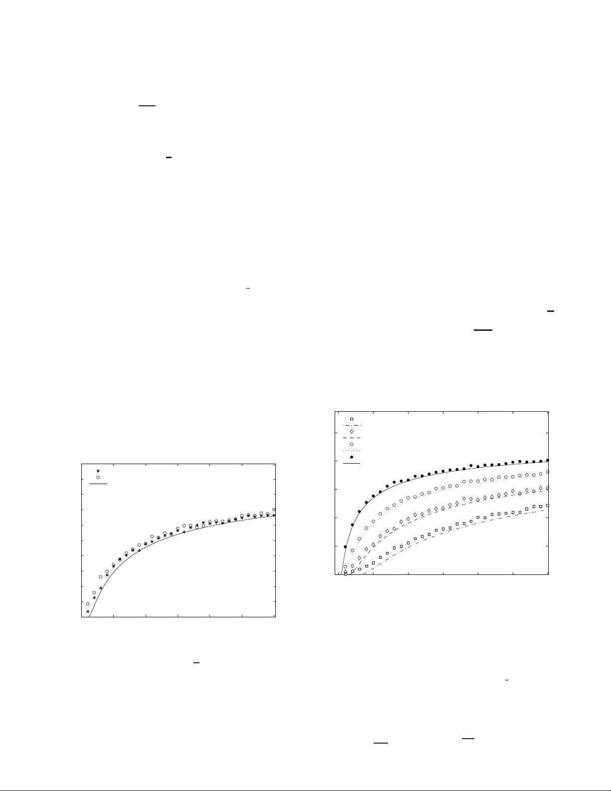
1 Correlate d Anarchy in Ov erlapping W ireless Netw orks Panayotis Mertikopoulos and Aris L. Moustaka s, Senior Member , IEEE Abstract —W e in vestigate the b eha vior of a large n umber of selfish users that are able to switch dynamically between multip le wireless access-points (possibly b elonging to di ff erent standards) by introducing an iterated non-cooperativ e game. Users start out completely uneducated and na ¨ ıve but, by using a fixed set of strategies t o process a bro adcasted train ing signal, they q uickly ev olve and con verge to an e volutionarily stable equilibrium. Then, in order to measure e ffi ciency in this steady state, we adapt t he notion of th e price of anarchy to our setting and we obtain an explicit analytic estimate for i t by using methods from sta tistical physics (namely the theory of replicas). Surprisingly , we find that the price of anarchy does not depend on the specifics of the wireless nodes (e.g . spectral e ffi ciency) b ut onl y on the n umber of strategies per user and a p articular combin ation of th e n umber of nodes, th e number of users and the size of the training signal. Finally , we map this game to the well-studi ed minority ga me , generalizing its a nalysis to an arbitrary number of choices. Index T erms —Wir el ess networks, Nash equil ibrium, correlated equilibriu m, price of anar chy , ev olutionary ga me, replicas I. I nt r o duction A S a result of t he massive dep loyment of IEEE 8 02.11 wireless networks, and in the pre sence of large-scale m o- bile third-g eneration systems, mobile users of ten h a ve several choices of overlapping networks to conne ct to. In fact, d evices that suppo rt multiple standards already exist an d, additionally , significant p rogress has b een made towards creating flexible radio devices cap able of c onnecting to any existing standard [1]. It is thus reason able to e xpect that, in the near futu re, users will be ab le to switch d ynamically between d i ff erent networks. In such a setting, ev en though users have se vera l choices to connect to, they st ill have to compete against each other for the finite reso urces of the combined ne twork. Hence, th is situation can be modelled using non- coopera ti ve game theory , a practice that is rapidly b ecoming one of the main tools in the analy sis of wir eless networks. For example, game- theoretic techniques were u sed to o ptimize transmission pr obabilities in [2 ] and to calculate the optima l po wer allocation [3]–[6 ] or the optimal transmitting carrier in [7]. The auth ors of [8] and [ 9] stud ied the possibility of co nnecting to several acc ess points using a single WLAN card; the selfish behavior of ser vice p roviders was an alyzed in [10]–[12] and, recently , ev en the e ff ects of pricing wer e e xamined in [13]–[1 6] using game the ory . P . Me rtik opoulos and A. Moustakas a re with the Physi cs Department, Nationa l and Kapodi strian Uni versity of Athe ns, 157 84 Athens, Greec e. This research was suppo rted in pa rt by t he European Co mmission under grants E U-MIRG-CT -20 05-030833 (PHYSCOM), EU-FE T -FP6-IST -034413 (NetReF ound) and EU-IST -2006-27960 (URANUS); the first author was also supported by the Em piriki on Founda tion of Athens, Greece. Part of this materia l was presented at the 2007 GameComm W orkshop in Nantes, France. The scen ario that we consider is an un regulated network where a large n umber of N heter ogeneo us users (e.g. mobile devices) connect wirelessly to one of B n odes (perhap s with di ff erent stand ards). All u sers wish to maximize their individ- ual d ownlink throug hput but ea ch ha s a di ff ere nt app roach: e.g. users m ay have di ff erent tolerance for d elay , or may wish to employ di ff erent “betting” schemes to do wnload data at the lowest pr ice. So, in gen eral, users have d i ff erent strategies, fixed at the outset of the game, and unknown to the r est. Now , given the u sers’ com petition fo r the no des’ limited resources, it is not cle ar how th ey can reach a n organ ized state in the ab sence o f a central coordin ating entity . One po ssible way to overcome this hu rdle is if users base their decisions o n a “training ” signal, e.g. a ra ndom signal that is synch ronou sly broadc asted by the n odes and received by all the u sers. Then, as this a ff air is iterated, one might hope that sophisticated users develop an in sight into h ow other users respond to the same stimulus and, e ventually , learn to coord inate their actions. This was pre cisely the sem inal ide a beh ind Aumann ’ s work in [17]: players ba se their d ecisions on th eir observations of the “states of th e world ” and reach a corr elated equilibrium . Similar games have als o been stu died in econop hysics, particularly after the introductio n of the El F ar ol pr oblem in [18] an d th e development o f the minority game in [19] . In both th ese g ames, play ers “buy” or “sell” and are rew arded when they lan d in the mino rity . Aga in, the key idea is that in or der to decide wh at to do, p layers re cord and process the game’ s history with the aid o f som e predeterm ined strategies. Then, b y employing mo re often the strategies th at p erform better, the y quick ly conver ge to an equilibriu m which ( in an unexpected twist) turns out to be obli vious to the source of the players’ observations [20]. In fact, it was shown in [21] that what matters is simp ly the amou nt o f f eedback th at play ers receive and the nu mber of strategies th ey use to process it. As in [ 22], our scen ario stands to gain a lo t from such an approach . Hence, our main goal will be to expoun d this scheme in a way app ropriate for selfish users in an u nregulated wireless network. The fir st step towards this is to gen eralize and adapt the mino rity g ame o f [2 1] to our setting: this is done in section I I wh ere we intr oduce the Simplex Ga me . Next, in section III, we char acterize the game’ s equilibr ia and comp are th em to the socially optimal state. From this compariso n emerges the game’ s price of ana r chy , a notion first described in [23] and which measur es the distance between anarchy (eq uilibria) and e ffi ciency (optima l states). Our first importan t result is obtained in section IV: by iterat- ing the g ame b ased on th e scheme of exponen tial learning, we 2 find th at playe rs conver ge to an evolutionarily stable equilib- rium (theorem 1 1). T hen, having establishe d convergence, we proceed in sectio n V to harvest the game’ s price of anarchy . Quite u nexpectedly , we find that th e price of ana r chy is unaf- fected by disp arities in the nodes’ c haracteristics (theorem 14). Moreover , we also deriv e an an alytic expression for the price of anar chy based on the m ethod o f replicas from statistical physics. Th is allows us to study the e ff ect of the various parameters o n the network’ s perf ormance, an analysis which we suppleme nt with numerical experime nts. As a byp roduct, this generalizes th e results of the tra ditional (bin ary) minor ity game to an arbitrary n umber o f cho ices. Some c alculational details th at would d etract o ne’ s fo cus from the ma in discussion h av e been defer red to the appen dices at the en d. Fin ally , as far as no tational conventions g o, we will den ote the standar d ( n − 1)-dimen sional simplex of R n by ∆ n = { x ∈ R n : x i ≥ 0 and P i x i = 1 } ; also, we will employ the game-theoretic sh orthand : ( x − i ; y ) = ( x 1 . . . y . . . x n ). II. T he S implex G ame T o model the scenario that we described in the intro duction, we conside r N users that may choose one of B nodes, each characterized b y a single user spectral e ffi ciency c r . In this case, if N r users connect to node r , their throug hput will be: T r = c r N r (1) (for simplicity we assume that users ha ve the same tran smis- sion ch aracteristics). Despite the simplicity of this thr oughp ut mo del, it has been shown to be of the correct form for TCP and UDP p rotocols in IE EE 80 2.11b systems, if we limit our selves to a single class of users [9]. Furthe rmore, in the case of third-g eneration best-e ff ort systems, the realistic total cell-service throughpu t is approx imately con stant beyond a certain number of connected users [24] . Thu s, (1) is a reasonab le app roximation fo r the user th roughp ut o f single- class mobiles. In fact, equ ation (1) is flexible eno ugh to accoun t f or parameters that a ff ect a user’ s bias tow ards a no de; e.g. we can incorp orate pricing by mod ifying c r to c r (1 − p r ) where p r reflects the price p er b it. So , we may ren ormalize (1) to: ˆ u r = y r N N r (2) where the coe ffi cients y r are normalized to unity ( P B r = 1 y r = 1) and rep resent the “e ff ective stren gth” of no de r in terms o f its attributes and character istics. Clearly , n odes can m odify this “strength” score, in or der to maximize their gain ; howev er , this is assumed to take p lace at slo wer time-scales and, hence, these strengths can be assumed to remain constant. 1 W e ma y no w note that the core constituents of a co ngestion game are all pre sent: N players (users) are asked to ch oose one of B facilities (nodes), their payo ff giv en by th e through put (2). From this standpoint, the “fairest” user distribution is the Nash allocation of y r N users to no de r : when distributed this way , u sers r eceiv e a payo ff of ˆ u 0 = 1 and no on e cou ld hope to earn m ore from a unilateral deviation (comp arably to the 1 Obviou sly , nodes of z ero strength (e.g. negligibl e spectral e ffi c ienc y) will not a ppeal to any reason able user a nd can be dropped from the ana lysis. “water -filling” of e.g . [25 ]). As a result, th e user s’ discom fort can b e g auged by contrasting their payo ff to the Na sh value: ˆ u r − ˆ u 0 = y r N y r N + N r − y r N − 1 = y r N − N r y r N + O (1 / N ) (3) So, if we focus on the leading term of (3) and introduce: u r = 1 − N r y r N (4) we may easily that th e Nash equilibr ia of th e game r emain in variant un der this linearization. In other words, the payo ff s (2) and (4) will be equi valent in terms of social fairness. 2 Thanks to this linearization , we may express a user’ s payo ff in a particular ly revealing form . Howe ver , to accomplish this, we first need to in troduce a collectio n of B vecto rs in R B − 1 with which to m odel the n odes: Definition 1 : Let y = ( y 1 . . . y B ) ∈ Int( ∆ B ) be a strength dis- tribution for B nodes. 3 A y -simple x (or y - appr o priate simplex ) is a co llection B = { q r } B r = 1 ⊆ R B − 1 such that, fo r r , l = 1 . . . B : q r · q l = − 1 + δ rl √ y r y l (5) Admittedly , this definition is rather opaque 4 but, fortunately , the ge ometric pictu re is much clear er: Lemma 2: Let B = { q r } B r = 1 be a y -appr opriate simplex for some y ∈ I nt( ∆ B ). Th en: P r y r q r = 0; also: P r y r q 2 r = B − 1. Pr oof: T o establish the first par t, no te that:  P B r = 1 y r q r  2 = P B r , l = 1 y r y l q r · q l = P B r , l = 1 y r y l  − 1 + δ rl  √ y r y l  = 0. As for th e second par t, it is ju st a straightforward app lication of (5). In other w ords, a y -simplex is just like a standar d simplex with vertices “weig hted” by th e streng ths y r . 5 So, if N r players choose q r , we may co nsider the aggr egate bet q = P B l = 1 N l q l and obtain b y (5): q r · q = P B l = 1 N l q r · q l = − N  1 − N r y r N  . W e then g et the very useful e xpression f or th e pay o ff (4): u r = 1 − N r y r N = − 1 N q r · q = − 1 N q r · P N i = 1 q r i (6) where r i indicates the choice of p layer i . In this way , lemma 2 shows th at Nash equilibria will be c haracterized by: q = P N i = 1 q r i = P B r = 1 y r N q r = 0 (7) i.e. the ga me will b e at equilib rium when the p layers’ choices balance out the weigh ts y r at the vertices of the simple x . Unfortu nately , it remain s u nclear how this Nash allocatio n can be ach iev ed in an u nregulated ne twork. For th is reason, we will introduc e a coord ination mechanism akin to the on e propo sed by Auman n in h is sem inal paper [17]. In a nu tshell, Aumann’ s scheme is that players o bserve the r andom events γ that transpir e in some samp le space Γ (the “ states of the world”) and then plac e their bets based on the se observations. In other words, players’ de cisions are ord ained by their ( cor- related) strate gies f i , i.e. fun ctions on Γ that conv ert events (“states”) γ ∈ Γ to actions ( betting sugg estions) f i ( γ ). 2 This is also v erified by our numerical e xperiments (see figure 1). 3 T o c lear up any con fusion: Int( ∆ B ) = { y ∈ R B : y r > 0 a nd P r y r = 1 } . 4 In fact, it is not ev en clear that the definition is not va cuous. This is shown in ap pendix A: y -simplices are pre tty easy to construc t for an y y ∈ Int( ∆ B ). 5 One could also ask here why we insist that y -simplices be embedded in R B − 1 instead of R B . T he reason for this is quite subtle and hinges on the fact that we need B to span the space it is embedded in, so that we may apply the Hubbard-Stratono vich transformation (see appe ndix B). 3 Inspired by [17] (and also [21 ]), w e propo se th at a broad- cast beacon transm it a training signa l m , d rawn from som e (discrete) sample space M . For exam ple, the nodes could be synchro nously b roadcasting the same integer m ∈ { 1 . . . M } , drawn from a un iform ra ndom sequen ce that is arb itrated e.g. by a governmen t agency such as the FCC in the US. T o process th is signal, u ser i h as at his disposal S B -valued random variables c i s : M → B ( s = 1 . . . S ): 6 these are the i th user’ s strate gies , used to convert th e signal m to an action c i s ( m ) ≡ c m i s ∈ B . So, if u ser i employs strategy s i , the collection of maps  c i s i : M → B  N i = 1 will be a c orrelated strategy in the sense of [1 7] (con trast with { f i } N i = 1 above). Howe ver, u nlike [17], we canno t assume that users d ev elop their strategies after car eful con templation on the “states of the world ”. Af ter all, it is quite u nlikely that a user will have much time to think in the fast-paced r ealm o f wireless networks. Consequen tly , when the gam e begins, we envision that each user rando mly “prep rogram s” S strategies, dr awn random ly from all the possible B M maps M → B . Of c ourse, since we a ssume users to be heter ogeneou s , they will pr ogram their strategies in wildly di ff erent w ays and independen tly of one ano ther . Still, rational users will exhibit a predispo sition tow ards stronger nodes; to account for this, we will posit that: P( c m i s = q r ) = y r (8) i.e. the probability that user i p r ograms n ode q r as response to the signal m is just the no de’ s stren gth y r . In e ff ect, strategies are picked in an ticipation o f competition with o ther u sers: specifically , if each u ser we re expecting to play alon e, h e would have picked strategies that lead to the strongest no de. W e may no w summ arize the above in a for mal definition: Definition 3 : Let y ∈ I nt( ∆ B ) be a strength distribution fo r B no des. Then, a y - appr o priate simplex game G consists of: 1) the set of players : N = { 1 . . . N } ; 2) the set of nodes : B = { q r } B r = 1 , where B is a y -simplex; 3) the set of signa ls : M = { 1 . . . M } , en dowed with the unifor m measu re  0 ( m ) = 1 M ; the ratio λ = M N will be called th e training parameter o f the game; 4) the set of strate gy choices : S = { 1 . . . S } ; also, f or each player i ∈ N , a probab ility measure p i ( s ) ≡ p i s on S ( P S s = 1 p i s = 1): these are the players’ mixed str a te g ies ; 5) a str ategy matrix c : N × S × M → B where c ( i , s , m ) ≡ c m i s ∈ B is the node that the s th strategy o f user i indicates as respon se to th e signal m ∈ M ; the entries of c are drawn rando mly based on: P( c m i s = q r ) = y r . Moreover , we endow Ω = M × S N with the produc t measure  0 × Q N i = 1 p i and define the f ollowing: 6) an insta nce of G is an e vent ω = ( m , s 1 , . . . s N ) of Ω ; 7) the bet o f play er i is the B - valued rando m variable: b i ( ω ) = c ( i , s i , m ); also, the aggr egate bet is: b = P N i = 1 b i ; 8) the pa yo ff for player i is the r .v .: u i = − 1 N b i · b . Thus, similarly to the minority game of [19] and [21], the sequence o f e vents that we in tuitiv ely envision is: 7 6 W e are assuming that S is the same for all users for the s ake of simplicity . 7 It is importa nt to note here that, for 2 ident ical nodes ( B = {− 1 , 1 } ), the simple x game reduces exa ctly to t he origin al minority game of [21]. • in the “initialization” phase (step s 1- 5), p layers program their strategies by drawing the strategy ma trix c ; • in step 6, the signal m is broad casted and, based on p i , players pick a strategy s ∈ S to process it with: p i s is the probability that user i employs his s th strategy; • in steps 7- 8, p layers con nect to the nodes tha t th eir strate- gies indicate ( b i ( m , s 1 . . . s N ) = c m i s i ) and recei ve th e linear payo ff ( 4): b y eq . (6), each of th e N r users tha t end up connectin g to n ode q r receives: − 1 N q r · P l N l q l = 1 − N r y r N ; • the game is iterated by repeating steps 6-8. As usual, the p ayo ff that cor respond s to th e (mixed) strategy profile p = ( p 1 . . . p N ) will be the multilinear extension : u i ( m , p ) = P { s } p 1 s 1 . . . p N s N u i ( m , s 1 . . . s N ). T o av oid carryin g cumberso me sums like this, we will follow the notation of [21] and use h·i to indicate expectations over a particular player’ s mixed strategy: h υ i i = P s p i s υ i s ; also, we will use an overline to denote av eraging over t he trainin g signals, as in: a = 1 M P m a m . III. S elfishness and E fficiency Clearly , th e on ly way that selfish u sers who seek to max- imize their individual throu ghput can come to an u nmedi- ated understan ding is by re aching a n equilibr ial state that discourag es unilateral deviation. But, since there is a palpab le di ff erence between the users’ strate gic d ecisions ( s ∈ S ) and the tactica l actions they take based on them ( c m i s ∈ B ), one would naturally expect the situation to be somewhat in volved. A. Notion s of Equilibrium Indeed , it should not c ome as a surp rise that th is dichotomy between strategies and action s is reflected on the gam e’ s equilibria. On the one han d, we h av e alre ady enco untered the game’ s tactical equilibrium : it corr esponds to the Nash alloca- tion of y r N u sers to n ode r . On the other ha nd, given that users only con trol the ir strategic choices, we should also examine Aumann’ s strategic notion of a co rr elated equilibrium . T o that end, recall that a correlated strategy is a collection f ≡ { f i } N i = 1 of maps f i : M → B (on e for each play er) that conv ert the signal m to a betting s uggestion f i ( m ) ∈ B . W e will then say that a ( pure) correlated strategy f is at equilibrium for player i when, for all p erturbatio ns ( f − i ; g i ) = ( f 1 . . . g i . . . f N ) of f , player i gains more (on average) by sticking to f i , i.e. u i ( f ) ≥ u i ( f − i ; g i ). When this is true for all players i ∈ N , f will b e called a corr elated equilibrium . As we saw be fore, if user i picks his s th i strategy , the collec- tion  c i s i : M → B  N i = 1 is a correlated strategy , b ut the con verse need not ho ld: in general, not every c orrelated strategy can be recovered from the limited num ber of prep rogram med strategic choices. 8 Thus, users will no longer be able to co nsider a ll perturb ations o f a gi ven strategy , and we are led to: Definition 4 : In the setting o f d efinition 3, a strategy pro file p = ( p 1 . . . p N ) is a constrained correlated equilibriu m when , for all strategy choices s ∈ S an d for all player s i ∈ N : 1 M P m u i ( m , p ) ≥ 1 M P m u i ( m , p − i ; s ) . (9) 8 There is a total of B M N correla ted s trate gies b ut users can recov er at most S N of them. In fact, this is why preprogramming is so useful: it w ould be highly unreasonabl e to expect a gi ven user to process in a timely f ashion the expo nential ly gro wing number of B M (as compa red to S ) strate gies. 4 The set o f all such equ ilibria o f G w ill be den oted by ∆ 0 ( G ). In our setting, a (con strained) co rrelated equilibrium is what r epresents anar chy: with no one to m anage the users’ selfish d esires, the only thing that deters th em fr om u nilateral deviation is their e xpectation of (average) loss. Conceptua lly , this is p retty similar to the notion of a Nash equilibrium, th e main di ff erence bein g that in a correlated equilib rium we are av eraging th e payo ff over the training signals. Th is analo gy will b e very useful to us and we will make it pr ecise by introdu cing th e correlated form of the simplex game: Definition 5 : The corr elated form of a simplex game G is a game G ∗ with the same set of pla yers N = { 1 . . . N } , each one choosing an action from S = { 1 . . . S } for a payo ff o f: u ∗ i ( s 1 . . . s N ) = 1 M P m u i ( m , s 1 . . . s N ) (10) In short, the payo ff that players r eceiv e in the co rrelated game is th eir throug hput averaged over a rotatio n of the training signals. Then, an imp ortant consequence of definition 4 is th at the constrained co rr elated eq uilibria of a s implex game G ar e pr e cisely th e Nash equilibria o f its corr ela ted form G ∗ . B. Harvesting the Equilibria So, our n ext goal will be to und erstand the Nash equilibria of G ∗ . T o be gin with, a brief calculation shows that the payo ff u ∗ i for a mixed pro file p = ( p 1 . . . p N ) is: u ∗ i ( p 1 . . . p N ) = − 1 N  h c i i · X j , i D c j E + D c 2 i E  (11) (the averaging notation s ( · ) and h·i being as in th e end of section II). Th us, g iv en the similar ities o f our gam e with congestion gam es, it might b e hoped that its Nash eq uilibria can be harvested by mean s of a potentia l fun ction , i.e. a function that m easures the payo ff di ff erence between u sers’ individual strategies [26]. More concr etely , a po tential U satisfies: u ∗ i ( p − i ; s 1 ) − u ∗ i ( p − i ; s 2 ) = U ( p − i ; s 1 ) − U ( p − i ; s 2 ) fo r any mixed profile p = ( p 1 . . . p S ) and any two strategic choices s 1 , 2 of p layer i . Ob viously th en, if a potential fu nction exists, its local maxima will be Nash equilib ria of the game . But, unfortun ately , since G ∗ does not h av e an e xact conges- tion structure, it is not clear how to con struct such a potential. Nev ertheless, a good candida te is th e game’ s aggregate payo ff u ∗ = P i u ∗ i . In fact, if player i cho oses strategy s , u ∗ becomes: u ∗ ( p − i ; s ) = − 1 N           P l , k , i l , k h c l i · h c k i + P k , i D c 2 k E + 2 c i s · P k , i h c k i + c 2 i s           . So, after some similar algebra for u ∗ i s ( p ) ≡ u ∗ i ( p − i ; s ), we o btain the follo wing compar ison between two strategies s 1 , s 2 ∈ S : u ∗ ( p − i ; s 2 ) − u ∗ ( p − i ; s 1 ) = 2 h u ∗ i s 2 ( p ) − u ∗ i s 1 ( p ) i + 1 N  c 2 i s 2 − c 2 i s 1  (12) Now , giv en th e preprogram ming (8) of c , we note that ( c m i s ) 2 takes on the value q 2 r = − 1 + 1 y r with pro bability y r . Hence, the central limit theorem (recall that M = λ N = O ( N )) implies that 1 M P M m = 1  c m i s  2 will h av e mea n P r y r ( 1 y r − 1 ) = B − 1 and variance 1 M P r  1 y r − B  , the latter being n egligible unless y is too clo se to the faces of ∆ B . More concr etely: Definition 6 : A distribution y ∈ Int( ∆ B ) is pr ope r when 1 B − 1 P B r = 1  1 y r − B  = o (1); other wise, y is called de generate . Hencefor ward, ou r work ing assump tion will be that there are no degenera te n odes: o therwise, we could simply remove them from th e analysis (i.e. red uce B and mo dify y accor d- ingly). This reflects the fact that degeneracy in the strength distribution simply indicates that certain no des have extremely low stren gth sco res and all reason able users shun the m. 9 W ith this in mind, the last term of (12) will be on average 0 and with a variance o f lesser order than the first term. Thus: u ∗ ( p − i ; s 2 ) − u ∗ ( p − i ; s 1 ) ∼ 2 h u ∗ i ( p − i ; s 2 ) − u ∗ i ( p − i ; s 1 ) i (13) i.e. the aggregate p ayo ff u ∗ is indeed a potential function for the ga me G ∗ (at least asymptotically). W e ha ve thu s p roven: Lemma 7: Let G be a simplex game for N p layers. Then, as N → ∞ , the maxima of the averaged aggregate u ∗ = P N i = 1 u ∗ i will co rrespon d (alm ost surely ) to correlated equilib ria of G . C. Anarc hy and E ffi ciency Still, one expects quite the gu lf be tween anarchic and e ffi cient states: af ter all, selfish players are hardly the on es to rely up on f or social e ffi cien cy . I n the context of networks, this con trast is frequen tly measured by the price of ana r chy , a no tion first introd uced in [23] as th e (co ordinatio n) ratio between the maximum attainable aggregate payo ff and the one attained at the game’ s equ ilibria. Then, depe nding on whethe r we loo k at worst or best-case equilibr ia, we g et the pessimistic or o ptimistic p rice o f anar chy respectively . In our game, the aggr egate p ayo ff is equal to: u = P N i = 1 u i = − 1 N P N i = 1 b i · P N j = 1 b j = − 1 N b 2 and attains a maximum of u max = 0 when b = 0. So, if w e recall by (7) that a Nash equ ilibrium occurs if and only if b = 0, we see that Nash a nar chy does not imp air e ffi ciency . Clearly , n either the users, no r the agencies that d eploy the wireless n etwork could ho pe f or a better so lution! Howe ver, this also shows that the traditional definition of the price of anarc hy is no lon ger suitab le fo r o ur purpo ses. One reason is that u max = 0 a nd, hence, we cannot hope to g et any info rmation fro m ratios inv o lving u max . 10 What’ s mor e, the users’ selfishness in o ur setting is m ore aptly c aptured by the Auman n equilibria of de finition 4, so we sho uld be taking the signal-averaged u ∗ instead of u . As a result, we are led to: Definition 8 : Let G be a simplex game fo r N players an d B nodes. Then, if p = ( p 1 . . . p N ) is a mixed strategy profile of G , we define its frustration level to be: R ( p ) = − 1 B − 1 u ∗ ( p ) = 1 N ( B − 1) 1 M P m b 2 ( p ) (14) that is, the (average) distance from the Nash solutio n b = 0. Also, the game’ s corr elated price o f anar chy R ( G ) will be: R ( G ) = inf n R ( p ) : p ∈ ∆ 0 ( G ) o (15) i.e. th e minim um value o f the fru stration level over the set ∆ 0 ( G ) of the game’ s con strained correlated equilibria. Some remark s are now in or der: first and forem ost, we see th at the frustratio n level of a stra tegy pro file measure s 9 After all , de generat e nodes cannot se rve more than o ( √ N ) users. 10 This actually highlights a general problem wit h the coord ination rat io: i t does not behav e well w .r .t. adding a co nstant to the payo ff fun ctions. 5 (in)e ffi cien cy by contrasting the average aggr egate pay o ff to the optimal case u max = 0 (the nor malization 1 B − 1 has been introd uced fo r future convenience). So, with correlated equilibria repre senting th e anarchic states of the game, we remain justified in the eyes o f [23] by calling R ( G ) the price of anarchy . In e ff ect, the only thing that sets us apart is that, instead o f a ratio, we are taking the di ff erence. Finally , one might wonder why we do not con sider th e pessimistic version by replacing the inf o f the above definitio n with a sup. The main reason f or this is th at in the n ext section, we will present a scheme with wh ich users w ill b e able to conv erge to th eir most e ffi cient equilibrium. Thu s, there is no reason to co nsider worst-case equilibria as in [23] : we only need to m easure th e price of sophisticated anarchy . IV . E volution and E quilibria Naturally , as the simplex gam e is iterated , one may assume that ra tional users will want to maximize their payo ff by employing more of ten the strategies th at perfo rm better . The most obvious way to accom plish th is is to keep track of a strategy’ s perf ormance and rew ar d it accordingly: Definition 9 : Let G be a simplex game as in definition 3, and let ω = ( m , s 1 . . . s N ) be an instance of G . Then, the r ewar d to the s th strategy of player i is the random variable: W i s ( ω ) = 1 M u i ( m , s − i ; s ) = − 1 M N c m i s · h b ( ω ) +  c m i s − c i s m i i (16) In o ther word s, the re ward W i s that player i awards to his s th strategy is ( a fractio n of) the payo ff th at the strategy would have gar nered for the player in the gi ven instance. 11 A seeming pro blem with the ab ove defin ition is that, in order to learn a nd evolve, u sers w ill have to rate all their strategies, i.e. they must be able to calculate the payo ff even of stra tegies they d id no t emp loy . So, given that the payo ff is a function of the aggregate bet b , it would seem that users w ould have to b e info rmed of e very o ther user’ s bet, a pr ospect that downright sha tters the unregulated p remises of o ur setting. Howe ver, a mo re carefu l conside ration o f (6) reveals that it su ffi ces for u sers to kn ow the distribution of users among th e nodes, somethin g which is small enough to be broadca sted by the nodes along with the signal m . 12 So, let u s conside r a sequ ence ω ( t ) of instances o f G to model the game’ s t th iteration ( t = 0 , 1 , 2 . . . ). At time t + 1, players rank th eir strate gies acco rding to their scores : U i s ( t + 1) = U i s ( t ) + W i s ( ω ( t )) (17) where we set U i s (0) = 0 to reflect that there is no a priori predisposition towards any gi ven strategy . Then, strategies are selected according to their scores, following the ev olu tionary scheme o f exponentia l lea rning (see e.g. [ 18], [2 7]) p i s ( t ) = e Γ i U i s ( t ) P s ′ e Γ i U i s ′ ( t ) (18) where Γ i represents the learnin g rate o f play er i . 11 The rescali ng facto r 1 M has been i ntroduced because significa nt rew ards should come only afte r checkin g a stra tegy aga inst at least O ( M ) signals. 12 Actuall y , the signal itself could be the user distribut ion of the previou s stage. This was discussed in [20] where the distinc tion between real an d fak e memory is seen to have a neg ligible impact on the game ’ s performance. As a fir st step to un derstand the dynamical system of (18), we no te that play ers’ ev olution actu ally takes place over the time scale τ = t / M : it takes an average of O ( M ) iterations to notice a distinct change in the scor es o f (16 ). In th is case, the score o f a strategy w ill have be en modified by : δ U i s = P τ + M t = τ W i s ( ω ( t )) = − 1 M N P τ + M t = τ  c m ( t ) i s · P j , i c m ( t ) j s j ( t ) +  c m ( t ) i s  2  . But, by applying the centra l limit theorem, we may write P j , i c m ( t ) j s j ( t ) ∼ P j , i D c m ( t ) i E and, un der so me mild ergodic- ity assumption s, we can a lso approx imate the time average 1 M P τ + M t = τ ( · ) by the ensemble a verag e 1 M P m ( · ). Thus, the change in a strategy’ s score after M iterations will be: δ U i s ∼ − 1 N  c i s · X j , i D c j E + c 2 i s  = u ∗ i ( p − i ; s ) (19) A fine poin t in the above is the implicit assump tion that p i s changes very slowly . This c av eat collap ses if the learning rates Γ i are too high (i.e. wh en we approach “hard ” best-response schemes) 13 but, if we stay away f rom this limit, we may pass to con tinuous time and di ff er entiate (1 8) to obtain: d p i s d τ = Γ i p i s  u ∗ i ( p ) − u ∗ i ( p − i ; s )  (20) since, b y (1 9), d U i s d τ will b e given by u ∗ i ( p − i ; s ). 0 50 100 150 200 250 0 0.5 1 1.5 Iterations Frustration Level Convergence to the Steady State Simplex Game (linearised) Random Case Simplex Game (capacity) Action Game Fig. 1. Simulatio n of a simplex game for N = 50 players that seek to connect to B = 5 nodes of random stregnth s with the help of M = 2 broadca sts and S = 2 strategie s. T he game is iter ated based on (18) with a learning rate of Γ i = 20, and we plot the users’ (insta ntaneo us) frustration R t = − u B − 1 (cf. (14)) versus the number of iteration s t : as predic ted by theorem 11 , players quickly con verge to a steady state of m inimal frustration . T o justi fy the linearisati on of (4), we a lso simulated a game wit h the nonlinea r payo ff (1), obtain ing virtually indisti nguishable results. As a baseli ne, we consider unsophistica ted users who simply pi ck a no de randomly , thus experienc ing much high er frustrat ion (on av erage R = 1). Finally , we also simulate rep licat or dynamics (with the s ame learni ng rate) on the congesti on game determin ed by (1 ); in that case, alt hough users e ventual ly reach the Nash solution, the y do so at a muc h slo wer rate. These d ynamics are extremely powerful: they are the stan- dard multi-pop ulation r eplica tor dyna mics fo r the corre lated form G ∗ of the gam e. T o be sure, in W eibull’ s extreme ly compreh ensiv e acco unt [29], it is shown th at they exhib it a striking equ iv alen ce: the asympto tically stable states 14 of ( 20) 13 See [28 ] for a detaile d discussion on this. 14 These are attract ing steady states t hat are also L yapunov stabl e. 6 are pre cisely th e (strict) Na sh eq uilibria of the u nderlyin g game (in our case G ∗ ). But, sinc e a strategy pro file is a Nash equilibriu m for th e corr elated game G ∗ if and on ly if it is a correlated e quilibrium fo r the original ga me G , this pr oves: Lemma 10 : Let G b e a simplex game, iter ated under (18). Then, almost surely as N → ∞ , a p rofile p = ( p 1 . . . p N ) will be asy mptotically stable w .r .t. the dy namics of ( 18) if a nd o nly if it is a constrained correlated equilibr ium of G . So, what remains to be seen is whether the learn ing sch eme of (18) r eally does lead the g ame to such a fo rtuitous state. T o tha t end, one w ould expect that, a s users e volve, the y learn how to m inimize their av erage frustration le vel and e ventually settle do wn to a stable local minim um. Roug hly s peaking , this is the co ntent of a Lyapunov fu nction , i.e. a fun ction L ≡ L ( p ) with d L d τ ≤ 0. If such a functio n exists, L y apunov’ s theo rem will e nsure conv ergence to the stead y state and, tha nkfully , there is an obviou s can didate: the aggregate p ayo ff u ∗ which is also the potential of the corre lated game G ∗ . Indeed , if we combine (13) and (20), we ca n see that: d u ∗ d τ = P i P s ∂ u ∗ ∂ p i s d p i s d τ = 1 2 P i Γ i P s u ∗ ( p − i ; s ) p i s  u ∗ ( p − i ; s ) − u ∗ ( p )  ≥ 0, the last step owing to Jensen’ s inequality (r ecall that u ∗ ( p ) = P s p i s u ∗ ( p − i ; s )) . In other word s, th e frustration R = − 1 B − 1 u ∗ is a L yap unov function for the d ynamics of (20) an d the play ers will co n verge to its glob al minimum; in e ff ect, this proves: Theor em 11 : If a simplex game G with a large number N of players is iterated un der the expone ntial learning scheme (18), the players’ mixed s trategies will conv erge almost surely to an asymptotically stab le state p ∗ with the following prope rties: (i) p ∗ is a (strict) constrained corr elated equilib rium o f G ; (ii) p ∗ is the most e ffi cient eq uilibrium o f G , in the sense that it maximizes the aggregate pay o ff u ∗ over all p ∈ Q N i = 1 ∆ S ; (iii) p ∗ is p ure. Pr oof: Thanks to the p receding discussion and L ya- punov’ s secon d theo rem, we only need to prove par t ( iii). But, since u ∗ is harm onic in p , it will attain its max imum value on on e of the vertices o f D = Q N 1 ∆ S . Then, seeing as p ∗ maximizes u ∗ by p art (ii), it must be pure. V . T he P rice of A narchy So far, we have seen that the dyn amics of expo nential learning lead the users to an ev olu tionarily stab le equilib rium which m aximizes (on average) their ag gregate payo ff (given their prep rogram ming). Hence , as far as measur ing anarchy is concern ed, we on ly ne ed to calculate the level of fr ustration at this steady state: rather surprising ly , it will tu rn o ut that the price o f anarch y is in depend ent o f the distribution y of the n odes’ strengths. In fact, the an alytic expression th at we obtain at the end of th is section shows that it is a fu nction only o f the num ber B o f nod es in the network , the tr aining parameter λ = M N and the number S o f strate gies per user . T o begin with, equ ation (11) fo r the fru stration level R at a mixed strategy pr ofile p can be re written a s: R ( p ) = 1 N ( B − 1) " X i D c 2 i E + X i , j i , j D c i E · D c j E # (21) So, recalling definitio n 6 and the discussion for the ag gregate payo ff (12), the first term of (2 1) will be: 1 N ( B − 1) P i D c 2 i E ∼ 1. Then, to dea l with the second term in (21), no te that for a giv en m , the aggregate bet b ( m , p ) = P i D c m i E giv es: b ( m , p ) 2 = P i P s p 2 i s  c m i s  2 + P i P s , s ′ p i s p i s ′ c m i s · c m i s ′ + P i , j i , j D c m i E · D c m j E . Thus, to lead ing o rder in N , this expression ha s an a verage of: 15 1 M X m b ( m , p ) 2 ∼ X i , j i , j D c i E · D c j E + ( B − 1) X i X s p 2 i s (22) As a result, eq uations (21 ) and (22) may be combined to: R ( p ) ∼ 1 + 1 M N ( B − 1) X M m = 1 b ( m , p ) 2 − G ( p ) (23) where G ( p ) = 1 N P i P s p 2 i s . By definition 8, the gam e’ s (optimistic) price o f anarch y R ( G ) will simply be the minimu m of R ( p ) over the game’ s equilibria. Bu t, sinc e th e minimum of R is an e quilibrium by theorem 11, we can simply take th e minimum over all mixed profiles: R ( G ) = min { R ( p ) : p ∈ Q N i = 1 ∆ S } . In this way , we g et a minimization p roblem of the kin d common ly encou ntered in statistical physics wh ere one seeks to harvest the g round states of (similar in form ) energy functio nals [30]. Motiv ated by this, we intro duce the partition fun ction : Z ( β, c ) = Z D e − β N R ( p ) d p (24) where D = Q N 1 ∆ S and d p = Q i , s d p i s is Lebesg ue measure on D . 16 In th is way , we may integrate asymptotically to wr ite: 17 R ( G ) = − 1 N lim β →∞ 1 β log Z ( β, c ) . (25) T o proceed, we will make the mild ( but importan t) assumption that, f or large N , it matters little which sp ecific strategy m atrix the user s actu ally picked. More form ally: Assumption 12 (Self-averaging): For any s trategy matrix c : log Z ( β, c ) ∼  log Z ( β )  all c (26) almost sur ely as N → ∞ (the averaging h·i takes p lace over all B N S M matrices c , drawn acc ording to (8)). This is a fu ndamental a ssumption in statistical ph ysics and describes the rar ity of c onfiguratio ns which yield notab le di ff erences in macr oscopically o bservable parameter s. Unde r this light, we are left to calculate  log Z  , a p roblem which we will attack with the h elp o f r eplica a nalysis . 18 The starting point of the method is the identity  log Z  = lim a → 0 + 1 a log h Z a i w hich reduces the prob lem to powers of Z : 19 R ( G ) = − 1 N lim β →∞ lim a → 0 + 1 a β h Z a ( β ) i (27) These ar e m uch mo re man ageable since, for n ∈ N : Z n = Z D e − β N R ( p ) d p ! n = Z D · · · Z D e − β N P µ R ( p µ ) Q µ d p µ (28) 15 See a lso [21] (pp. 529) for more on this point. 16 Z depends on the strateg y matrix c through the frustration le vel R ( p ). 17 Essentiall y , this re fers to the fact tha t max D f = lim x →∞ 1 x log R D e x f ( t ) d t for any measurable function f on a co mpact domain D (see e.g. [31]) . 18 See [30 ] for a general di scussion or [21], [32] for the minori ty game. 19 T o pr ov e thi s identit y , write Z a = e a lo g Z and e xpand. 7 i.e. Z n = Q n µ = 1 Z µ , where Z µ = R D exp  − N β R ( p µ )  d p µ is the partition functio n for the µ th r ep lica p µ = { p i s µ } o f the system. Th en, th anks to equation (2 3), we obtain:  Z n ( β )  = A n Z D n  e − β M ( B − 1) P µ P m ( c m µ ) 2  e N β P µ G µµ ( p ) Q µ d p µ (29) where A = e − N β ; c m µ = b ( m , p µ ) = P i P s p i s µ c m i s is the aggr egate bet for the mixed profile p µ = { p i s µ } in the µ th replica (giv en the signal m ); and G µν ( p ) = 1 N P i P s p i s µ p i s ν . Of cou rse, wh at we really ne ed is to e xpress h Z n i f or real values o f n in the vicinity of n = 0 + ; f or th is, we resort to : Assumption 13 (Replica Continuity): Th e e xpression g i ven in (29) for  Z n  can be co ntinued analytically to all real values of n in th e vicinity of n = 0 + . At first glance, this migh t appe ar as a blind leap of faith, especially sinc e u niquene ss criter ia (e .g. lo g-conve xity) are absent. Ho wever , such criteria can in so me cases be established (see e .g. [3 3]) an d, mo reover , th e h uge am ount of literature surroun ding th is assum ption and the agreemen t of our own analysis with our numerical results (see fig ures 2 – 5) makes u s feel justified in employing it. W ith the help of th e above, an d after the lengthy calculations of ap pendix B , we are in a position to prove: Theor em 14 (Irr elevance o f No de Strengths): Let y , y ′ ∈ Int( ∆ B ) be stre ngth distributions f or B nod es and let G , G ′ be simplex game s for y an d y ′ respectively . Then , as N → ∞ : R ( G ) ∼ R ( G ′ ) (30) In o ther words, we are (rather unexpected ly!) r educed to the sym metric case of B equiv a lent nodes: ceteris paribus, the price of an ar chy depends o nly o n the nu mber o f n odes pr esent and not on their individ ual str en gths . 0 0.5 1 1.5 2 2.5 3 0 0.1 0.2 0.3 0.4 0.5 0.6 0.7 0.8 0.9 1 λ Price of Anarchy Independence on Node Strength Symmetric Simplex Arbitrary Simplex Theory Fig. 2. The price of anarchy (i.e. the steady-st ate frustration lev el) as a function of the training paramete r λ = M N for B = 4 equi v alent nodes contrast ed to that of 4 nodes employing s tandar ds with di ff erent spectra l e ffi cienc ies c r : E VDO-Re v .A (1.06 Mbps), HSDP A (3.91 Mbps), 802.11b (11Mbps) and W iMAX (14.1 Mbps) [34]; we simulated N = 50 users with S = 2 strat egi es and a veraged o ver 25 realizatio ns of the game. As p redicte d by the orem 14, di ff erent standar ds do not a ff ect the pric e of anarchy . Now , in order to a ctually determ ine the e ff ect of choices on the u sers’ fr ustration level, we fir st d efine th e bina ry reduction of a simplex g ame G fo r B nodes. This is just a simp lex game G e ff for 2 id entical nodes and a tr aining set enlarged by B − 1, i.e. M e ff = M ( B − 1); everything else r emains the same. T hen, under this rescaling, the same train of calculations th at is u sed to pr ove theo rem 14 also yield s: Theor em 15 (Reduction of Choices): The price of a narchy for a simplex game G is asympto tically equal to that of its binary r eduction G e ff ; in other word s, as N → ∞ : R ( G ) ∼ R ( G e ff ) (31) Thanks to this eq uiv alen ce, we see that the p rice of anarchy depend s on M and B only thro ugh M ( B − 1); so, for example , if some nodes go o ffl ine, we will know exactly ho w muc h to increase M so as to maintain th e same perform ance level. Howe ver, theorem 15 really tells us much mor e: it provides a “dictio nary” betwe en the simp lex game an d the extensi vely studied minority game. Indeed, mutatis mutandis, one sees that the price o f anarch y R ( G ) correspon ds to the market volatility σ in the m inority gam e [21] . So, if we follow the ( r ep lica- symmetric ) calculations of [21], we finally ob tain the p rice o f anarchy in terms of the g ame’ s p arameters B , S an d λ = M N : R ( G ) ∼ Θ ( λ − λ c )  1 − p λ c  λ  2 (32) where Θ is the Hea viside step function and λ c = λ ( S , B ) is the critical value th at mark s the emergence of anarc hy within th e premises o f rep lica symm etry (see appendix B). 20 0 0.5 1 1.5 2 2.5 3 0 0.2 0.4 0.6 0.8 1 λ Price of Anarchy B=2 B=2 (theory) B=3 B=3 (theory) B=5 B=5 (theory) B=10 B=10 (theory) Fig. 3. The e ff ect of cho ices: we plot the price of anarchy as a funct ion of the training parameter λ = M / N for N = 50 users, S = 2 s trate gies and B = 2 , 3 , 5 , 10 nodes (ave raging ove r 25 realizati ons). W e see that e ffi cienc y deterio rates as B increases: more choi ces act ually confuse the users. This expression is one of our key results since it ac curately captures th e imp act o f th e various system para meters on the network ’ s perf ormance (see e.g . figures 2 – 5). So, even though it follo ws e ff ortlessly by vir tue of theo rem 1 5, for the sake of completeness (and also to discuss the role of r eplica symmetry ), we carry out the d eriv atio n of (3 2) in appen dix B. 20 Actuall y λ c = ζ 2 ( S ) B − 1 with ζ ( S ) = S  2 S − 1 √ 2 /π R ∞ −∞ ze − z 2 erfc S − 1 ( z ) d z ). 8 0 0.5 1 1.5 2 2.5 3 0 0.1 0.2 0.3 0.4 0.5 0.6 0.7 0.8 0.9 1 λ Price of Anarchy S=2 S=2 (theory) S=3 S=3 (theory) S=4 S=4 (theory) Fig. 4. The e ff e ct of sophisticat ion: we plot the price of anarchy as a funct ion of the traini ng paramete r λ = M / N for N = 50 users, S = 2 , 3 , 4 s trate gies and B = 5 nodes (again averag ing over 25 realizati ons of the game). A s expecte d, sophistic ated users (lar ger S ) are more e ffi cie nt. 0 0.5 1 1.5 2 2.5 3 0 0.2 0.4 0.6 0.8 1 λ Price of Anarchy N=10 N=25 N=50 N=100 theory Fig. 5. The price of anarchy as a function of the trainin g paramete r λ = M / N for di ff erent numbers of users N = 10 , 25 , 50 , 100, with B = 5 nodes and S = 2 strate gies; unl ike other plots, we are harvesti ng the price of anarchy from a single realizati on of the game. W e see that th e number of players does not seriously i mpact the p rice of anarchy (e xcept through λ ). VI. C onclusions Our main goal was to analyze a n unr egulated n etwork of (a large n umber of) heterog eneous users that can con nect to a multitude of wireless n odes with di ff erent specification s (e.g. di ff erent standards). In su ch a n etwork, u sers who selfis hly try to maximize their indi vidual do wnlink throug hput (2) will ha ve to compete again st each other for the n odes’ finite resour ces. So, in the pur suit o f o rder (and in the absen ce o f a central overseer), we a dvocate the use of a training beaco n (such as a random integer sy nchron ously b roadcasted by the n odes) to act as a coordin ation stimulus: b y processing this stimulus with the aid of some preprogram med strategies and choosing a node accordin gly , users should b e able to re ach an equilibrium. Indeed , if users keep records of their strategies’ performance and rank them based on the evolutionary sch eme of expo- nential learning (18), they learn to co ordinate their actions and quickly reach an evolutionarily stab le state. 21 This state is also socially stable in the sense that unilater al de v iation is (on av erage) discouraged: it is a corr elated equilibrium . Then, to measure the e ffi ciency of users in this setting, we examine ho w far they are f rom the optimal distribution th at maximizes their aggregate throu ghput. I n so d oing, we see tha t exponential learning lea ds th e users to their most e ffi cient equilibrium . Howe ver, since the u sers’ rationality is boun ded (i.e. they can only handle a sma ll num ber of strategies), this equilibrium will still be at some distance f rom the optimal state. This distance is the price o f ( corr ela ted) anarc hy an d we calculate it with the metho d of re plicas. In terestingly , we find (theo rem 14) that the price of an ar chy doe s not depend on the nodes’ characteristics, b ut only on their n umber . In f act, we provide a reduction of our scenario to th e minority gam e [19] (theor em 15) and, as a result, we obtain the analytic expression (3 2) for the price of a narchy . This also gen eralizes the results o btained for the m inority g ame to an ar bitrary nu mber of choices. Thanks to the ab ove, we d erive quantitative predictio ns about the degree of anarchy in our scenario. For example (fig. 3), we see th at blindly adding mo re nodes to a ne twork is not a panacea: anarchy actually incr eases with the number of nodes because the users are not able to process the added complexity and do not make e ffi cient use of the extra r esources. On the other h and, if users becom e more sophisticated and emp loy more strategies (fig. 4) , anarchy co mes at a lesser p rice (albeit at a slower conv ergence to a stab le state). Finally , we see th at the n umber o f user s r eally do esn’t have to b e qu ite so large (fig. 5): these con clusions hold ev en fo r the much sma ller number s of u sers ty pically encoun tered in local service areas. A ppendix A P r o per ties of y -S implices W e begin here b y showing that definition 1 is no t vacuou s: Lemma 16 : There exists a y -simplex B = { q r } B r = 1 ⊆ R B − 1 for any y ∈ Int( ∆ B ). Pr oof: Begin b y selecting a vector q 1 ∈ R B such that q 2 1 = 1 y 1 − 1 an d ch oose q r + 1 ∈ R B inductively so that it satisfies (5) wh en mu ltiplied by q 1 . . . q r . Su ch a selection is always possible f or r ≤ B − 1 thank s to the dimension of R B ; f or a vector space of lesser dimensio n, this is no longer the case. 22 In th is way , we obta in B vectors q r ∈ R B that satisfy (5); our co nstruction will b e com plete once we show that B is contained in some ( B − 1)-sub space o f R B . Howev er , as in the proof of lemma 2, we can see that P B r = 1 y r q r = 0; this m eans that B is linearly depe ndent and completes our proof. The n ext lemma is a key prop erty of y -simplices th at plays a crucial role in th e calculations of appendix B: 21 In fi gure 1 we see that con vergenc e occurs within tens of iteration s. Thus, if ea ch itera tion is of th e orde r of milli seconds (a reasona ble transmission timescal e for wideband wireless netw orks), this corresponds to equilibra tion times of tens of milliseconds. 22 Note that 1 y r y l ≥ 1 y r + 1 y l for all r , l so that q 2 r · q 2 l ≥ ( q r · q l ) 2 holds for (5). 9 Lemma 17 : Let B = { q r } B r = 1 ⊆ R B − 1 be a y -simp lex f or some y ∈ Int( ∆ B ). Then, for all x ∈ R B − 1 : P B r = 1 y r ( q r · x ) 2 = x 2 . Pr oof: Since y ∈ Int( ∆ B ), B will span R B − 1 and x may be written as a linear co mbination x = P B r = 1 x r q r . So , if we let S = P B r = 1 x r and recall that P B r = 1 y r = 1, we will h av e: x 2 = P B l , r = 1 x l x r q r · q l = − S 2 + P B r = 1 x 2 r / y r . Similarly : ( q r · x ) 2 = S 2 − 2 S x r y r + x 2 r y 2 r , and an addition over r yields th e lem ma. A ppendix B M easuring the P rice of A n archy Picking up whe re we left o ff in sectio n V, we begin b y calculating the expr ession for h Z n i in (2 9). T o do this, we will use the iden tity: e − q 2 2 = 1 ( 2 π ) k / 2 R R k e i q · z − z 2 2 d z = E z e i q · z where E z denotes e xpectation ov er a Gaussian r andom vector z with k in- depend ent components z 1 . . . z k ∼ N (0 , 1); this is the Hubba r d- Stratonovich transfo rmation. So, if n z m µ = ( z m µ, 1 . . . z m µ, B − 1 ) o m = 1 ... M µ = 1 ... n are such vectors of R B − 1 , we get:  e − β M ( B − 1) P µ P m ( c m µ ) 2  = E { z m µ }  e i P i P s P m x m i s · c m i s  (33) where: x m i s = q 2 β M ( B − 1) P µ p i s µ z m µ ∈ R B − 1 . Then, by the in- depend ence of th e c i ’ s (eq. (8)), we will b e able to ob tain the average h·i o f (33) over th e matrices c by compu ting the characteristic functio n D e i x · q E for on ly on e of them. Th is is done in the following: Lemma 18 : Let y ∈ Int( ∆ B ) and let B = { q r } B r = 1 be a y - simplex in R B − 1 . If x ∈ R B − 1 and q is a rando m vector with distribution P( q = q r ) = y r , then: D e i x · q E = e − x 2 2 + O  | x | 3  . Pr oof: Expanding the exponential  exp(i x · q )  yields: D e i x · q E = D 1 + i x · q − 1 2 ( x · q ) 2 + O  | x | 3 E = 1 + i x · P r y r q r − 1 2 P r y r ( q r · x ) 2 + O  | x | 3  = 1 − 1 2 x 2 + O  | x | 3  = e − 1 2 x 2 + O  | x | 3  (34) where the th ird eq uality c omes fr om lemmas 2 and 17. In ou r case, | x m i s | = O ( M − 1 2 ); so , if we ap ply the previous lemma to each of th e rand om vectors c m i s , the average of eq . (33) will becom e (to lead ing order in N ):  e i P i P s P m x m i s · c m i s  ∼ e − 1 2 P i , s , m ( x m i s ) 2 = e − β λ ( B − 1) P m P µ,ν G µν ( p ) z m µ · z m ν (35) where λ = M N is the game’ s training par ameter . Now , if we intro duce the n × n matrix J = I + 2 β λ ( B − 1) G ( p ), and r ecall that R R n e − 1 2 P µ,ν J µν w µ w ν f d w = | det( J ) | − 1 2 , 23 we may integrate over the auxiliary variables z m µ to ob tain: E z m µ  e − β M ( B − 1) P µ P m ( c m µ ) 2  ∼ Z R n M ( B − 1) e − 1 2 P M m = 1 P B − 1 k = 1 P µ,ν J µν ( p ) z m µ, k z m ν , k e d z = Z R n e − 1 2 P µ,ν J µν ( p ) w µ w ν f d w ! M ( B − 1) = e − M ( B − 1) 2 log det ( J ( p ) ) (36) So, after these c alculations, equation (29) finally becomes: h Z n ( β ) i A n ∼ Z D n e N β h tr( G ( p )) − λ ( B − 1) 2 β log det  I + 2 β λ ( B − 1) G ( p ) i Q µ d p µ (37) 23 Here, ti ldes as in f d w den ote Lebesgue m easure normalized by √ 2 π . Clearly , this last expression is indepe ndent of the stren gth distribution y , a fact which proves theorem 14. In add ition, we observe that (37) remains in variant when we pass from th e game G to its bin ary redu ction G e ff with the rescaled trainin g parameter λ e ff = λ ( B − 1), thus proving theor em 15 as well. Now , t o p roceed fro m (37), we will introduce n 2 δ -func tions in their integral representatio n so as to isolate the pro files p i s : δ ( Q − G ( p ) ) =  N β 2 π  n 2 R e iN β P µ,ν k µν ( Q µν − G µν ( p ) ) Q µ,ν d k µν . In this way , the integral o f (3 7) beco mes: Z e − N β h λ ( B − 1) 2 β log det  I + 2 β λ ( B − 1) Q  − tr( Q ) − i P µ,ν k µν ( Q µν − G µν ( p ) ) i d σ (38) where d σ = Q µ d p µ × Q µ,ν d k µν × Q µ,ν d Q µ,ν is th e product measure on D n × R n 2 × R n 2 . Howe ver, p only appear s in the last term of th e ( 38) and can be integrated separately to yield : Z D n e − i N β P µ,ν k µν G µν ( p ) Q µ d p µ = N Q i = 1       Z ∆ n S e − i β P µ,ν k µν P s p i s µ p i s ν Q s ,µ d p i s µ       = e xp       N log Z ∆ n S e − i β P µ,ν k µν P s p s µ p s ν Q s ,µ d p s µ       (39) (recall th at G µν ( p ) = 1 N P i P s p i s µ p i s ν and D n = ( ∆ S ) N × n ). So, by d escending to the limit N → ∞ , we find: 1 N log h Z n ( β ) i ∼ − β  n + λ ( B − 1) 2 β log d et  I + 2 β λ ( B − 1) Q  − tr( Q ) − − i P µ,ν k µν Q µν − 1 β log Z ∆ n e − i β P µ,ν k µν P s p s µ p s ν Q s ,µ d p s µ  ≕ − β Λ (40) where Q and k extremize th e fun ction Λ with in the b rackets. This is where we will inv oke r eplica symmetry (see [30] , [32]). Assumption 19 (Replica Symmetry): T he sa ddle-po ints of Λ a re of the f orm: Q µν = q + ( Q − q ) δ µν ; k µν = i λβ B − 1 2  r + ( R − r ) δ µν  (41) In o ther words, we seek sad dle-poin t matrices that are sym- metric in the replica space (the scalin g factor s are ther e for future co n venience). 24 Under this ansatz, we obtain : Λ = n + λ ( B − 1) 2 β log det  2 β λ q B − 1 +  1 + 2 β λ Q − q B − 1  δ µν  − n Q + n λβ B − 1 2 ( QR − q r ) + n 2 λβ B − 1 2 qr − 1 β log Z ∆ n e λβ 2 B − 1 2  ( R − r ) P µ p 2 µ + r ( P µ p µ ) 2  Q s ,µ d p s µ (42) where p µ is the generic pro file ( p 1 µ . . . p S µ ) in th e µ th replica. The second term of the ab ove expression c an be easily calculated by noting that det  q + p δ µν  = p n  1 + n q p  : it will be equal to q 1 + χ + λ 2 β ( B − 1)lo g (1 + χ ) + o ( n ), where χ = 2 β λ Q − q B − 1 . As for the last term of (42), we will again use the Hubbard - Stratonovich tran sformation with a cano nical Gaussian vari- able z of R S to write: e r λβ 2 B − 1 2 ( P µ p µ ) 2 = E z e − β √ r λ ( B − 1) z · P µ p µ . Then, fo r no tational convenience, we also let: V ( z , p ) = √ r λ ( B − 1) z · p − λβ B − 1 2 ( R − r ) p 2 (43) 24 This assumption can actually be dropped; e.g. see [32] where the first step of symmetry br eaking (1RSB) is performed. Stil l, replic a symmetry doe s no t incur a significant erro r on our calcula tions while great ly simplifying them. 10 and, in th is way , the integral of (42) beco mes (d p = Q S 1 d p s ): log E z Z ∆ n S e − β P µ V ( z , p µ ) Q s ,µ d p s µ = n E z log Z ∆ S e − β V ( z , p ) d p + o ( n ) From (27) an d th e premises o f replica contin uity (assum p- tion 1 3), what we really need to calcu late is Λ 0 = lim n → 0 1 n Λ : Λ 0 = 1 + q 1 + χ + λ 2 β ( B − 1) lo g(1 + χ ) − Q + λβ B − 1 2 ( QR − q r ) − 1 β E z " log Z ∆ S e − β V ( z , p ) d p # (44) where Q , q , R , r have been chosen so as to satisfy the r eplica- symmetric sad dle-point e quations: ∂ Λ 0 ∂ Q = 0, ∂ Λ 0 ∂ q = 0, etc. T o that e nd, it can b e shown th at bo th Q − q and R − r are of or der O (1 /β ), i.e. χ rema ins finite as β → ∞ . So, in this limit, we will o nce again perf orm asymptotic inte gration for the in tegrals o f ∂ Λ 0 ∂ R = 0 an d ∂ Λ 0 ∂ r = 0. Thus, we are led to consider th e vertex p ∗ ( z ) o f ∆ S which min imizes the harmon ic function V ( z , · ) and we obtain : Q ∼ φ R = r + 1 β 2 λ ( B − 1) χ 1 + χ (45) q ∼ φ + 1 β ζ √ λ ( B − 1) r r = 4 λ 2 ( B − 1) 2 1 (1 + χ ) 2 where φ = E z [ p 2 ∗ ( z )] and ζ = E z [ p ∗ ( z ) · z ]. Now , if we let β → ∞ an d substitute (45) in (44), we get Λ 0 = 1 − φ + φ  1 + ζ . p φλ ( B − 1)  2 where, af ter a little geome- try: ζ ( S ) = E z [min { z 1 . . . z S } ] = S 2 S − 1 q 2 π R ∞ −∞ ze − z 2 erfc S − 1 ( z ) d z and φ = 1. Hence, f or finite χ (i.e. fo r λ ≥ λ c = ζ 2 ( S ) B − 1 ), we finally acquire expression (32) for the game’ s price of anar chy : R ( G ) ∼ Λ 0 ∼ Θ ( λ − λ c )  1 − q λ c  λ  2 . R eferences [1] P . Demestichas, G. V i vier , K. El-Khazen, and M. T heologou , “Evolu- tion in wirel ess systems management co ncepts: from composite radio en vironments to reconfigur abilit y , ” IEEE Communicati ons Magazi ne , vol. 42, no. 5, pp. 90– 98, May 2004. [2] A. B. Ma cK enzie and S. B . Wi cke r , “Selfish users in ALOH A: A game theoret ic approach, ” IEEE Comm. M agazine , vol. 126, p. 126 , Nov . 200 1. [3] N. Bonneau, E. Altman, M. Debbah, and G. Caire , “ An evol utionar y game perspecti ve to ALOHA with power control , ” P r oceed ings of the 19th International T elet ra ffi c Congr ess, Beijing , China , Aug. 2005. [4] D. P . Palomar , J.M.Cio ffi , and M. Lagunas, “Unifo rm po w er all ocation in MIMO chann els: a game-theoreti c approach, ” IEEE T rans. Info rm. Theory , v ol. 49, no. 7, p. 1707, Jul. 2003 . [5] F . Meshkati, H. V . Poor, S. C. Schwartz, and N. B. Mandayam, “ An energy-e ffi c ient ap proach to power control and re cei ver design in wireless da ta netw orks, ” vo l. 53, no. 11, p. 1885, No v . 2005. [6] N. Bonneau, M. Debbah, E. Altman, and A. Hjorungne s, “W ardrop equili brium for CDMA syst ems, ” in R awnet , 2007. [7] F . Meshkati, M. Chiang, V . Poor, and S. C. Schwar tz, “ A game- theoret ic approach to energy-e ffi c ient power control in multicarrie r CDMA systems, ” IEEE Jo urnal on s elec ted ar eas in communicati ons , vol. 24, pp. 1115–1129, 2006. [8] R. Chandra , P . Bahl, and P . Ba hl, “Mult iNet: Connect ing to multiple IEEE 802.11 netw orks using a single wirel ess card, ” Proc. IEEE Infoco m 2004 , Mar . 200 4. [9] S. Shakkotta i, E. Altman, and A. Kumar , “Multihoming of users to access points in WLANs: A population game perspecti ve, ” IEE E J . Selec t. Areas Commun. , vol . 25, no. 6, p. 1207, Aug. 2007. [10] M. M. Halldorsson, J. Y . Halpern, L. (Erran) L i and V . S. Mirrokni, “On Spectrum Shar ing Games, ” P r oceed ings of PODC’ 04 . [11] A. Z emliano v an d G. de V ec iana, “Cooperat ion and Decision Making in W ireless Mult i-Provi der Setting, ” Pr oceedi ngs of INFOCOM’ 05 . [12] M. Felegyh azi, M. Cagalj, D. Dufour a nd J.-P . Hubaux, “Border Games in Ce llular Netw orks, ” Procee dings of INFOCOM’ 07 . [13] S. Shakkott ai and R. Srikant, “Economics of network pricing with multiple ISPs, ” IEEE / ACM T rans. Netw . , v ol. 14, no. 6, p. 1233, 20 06. [14] R. E. Azouzi, E. Altman, and L. W ynter , “T elecommunicat ions netw ork equili brium with price and quality- of-service character istics”, Proc . ITC, Berlin, German y , Sep. 2003. [15] L. He and J. W alra nd, “Pricing and re venue sharing strate gies for internet service provider s, ” IEEE J. Select. Ar eas Commun. , v ol. 24, no. 5, p. 942, May 2006. [16] J. Huang, R. Berry , and M. L. Honig, “ Auction -based spectrum sharing, ” ACM MONET , v ol. 11, no. 3, Jun. 2006. [17] R. J. Aumann, “Subjecti vity an d Correlation in Randomized Strategie s”, J ournal of Mathematic al Economics , vol. 1, no. 1, Mar .1974, pp. 67–96. [18] W . B. Arthur , “Inducti ve reasonin g and bounded rationalit y (the El Farol problem), ” Am. Econ. A ssoc. P apers Pr oc. , vol. 84, pp. 406–411 , 1994. [19] D. Challet and Y .-C. Zhang, “On the minority game: Analytic al and numerica l studies, ” Physica A , vol. 246, pp. 407–418, 1997. [20] A. Ca vagna, “Irre le vance of m emory in the minority ga me, ” P hys. R ev . E. , v ol. 59, pp. 3783–3786, 1999. [21] M. Marsili, D. Cha llet, and R. Zecchina , “Exact solution of a modifie d El Farol ’ s bar problem: E ffi ci ency and the role of market impact, ” P hysica A , vol. 280, pp. 522–553, 2000. [22] A. Galstyan and K. Lerman, “ Adapti ve Boole an ne tworks and minor- ity games with time-dep endent capacitie s, ” Phys. R ev . E , vol. 66, p. 0151103R, 2002. [23] E. Koutsoup ias and C. Papadi mitriou, “W orst-case equilibria. ” in Pro- ceedi ngs of the 16th Annual Symposium on Theoreti cal Aspects of Computer Sc ience , pp. 404–413, 1999. [24] A. G. K ogiant is, N. Joshi, and O. Sunay , “On tra nsmit di versity and scheduli ng in wireless pac ket data, ” Pr oc. IEEE ICC , vol. 8, pp. 2433– 2437, Jun. 2001. [25] L. Lai and H. El Gamal, “Fad ing Multiple Access Channels: A Game Theoretic Perspe cti ve, ” Proc. IEEE ISIT , pp.1334–1338, July 2006 . [26] D. Monderer and L.S. Shapley , “Potenti al Games”, Games and Eco- nomic Behav ior , vo l. 14, pp. 124–143, 1996. [27] A. Rustichini, “Optimal properties of stimulus-response learning mod- els, ” Game s and E conomic B ehavior , vol. 29, p. 244(30), 19 99. [28] M. Marsi li and D. Ch allet , “Continuum ti me limit and stat ionary sta tes of the minority game, ” Phys. Rev . E , vol . 64, 056138, Oct 20 01. [29] J. W eibu ll, Evolu tionary Game The ory . The MIT Press, 1995. [30] H. Nishimori, Statisti cal Physics of Spin Glasses and Information Pr ocessing . Oxford Unive rsity Press, 200 1. [31] A. Dembo an d O. Zeit ouni, Lar ge Deviatio ns T echn iques and Appli ca- tions . Springer -V erlag, 1998. [32] A. de Martino and M. Marsili, “Replica symmetry breaking in the minority game, ” J. Phys. A: Mathemat ical and General , vol. 34, no. 12, pp. 25 25–2537, 2001. [33] A. Coolen, The mathemat ical theory of minority games . Oxford Uni versi ty Press, 2004. [34] “Mobile W iMAX No2: Comp. Anal ysis, ” WIMAX F orum , May 2006.