Throughput and Delay Analysis of Wireless Random Access Networks

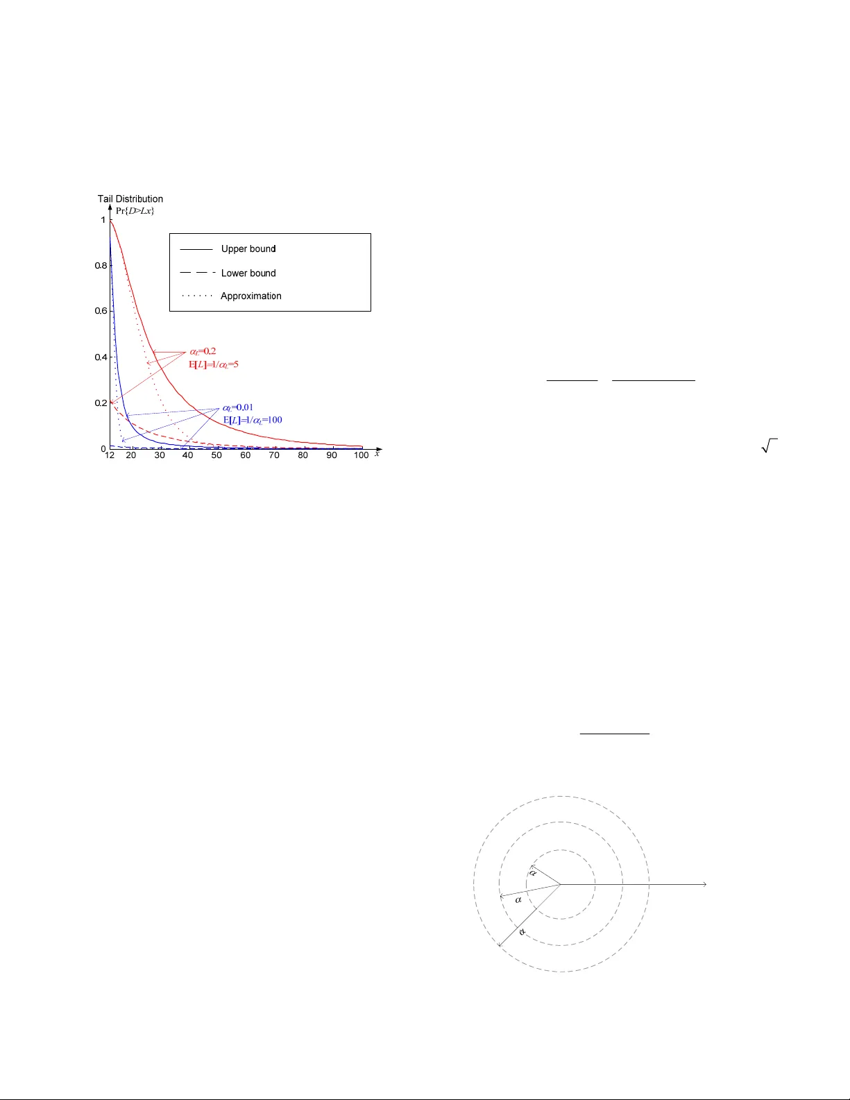
DAI AND LEE: THROUGHPUT AND DELAY ANALYSIS OF WIRELESS RANDOM ACCESS NETWORKS 1 Throughput and Delay Analysis of W ireless Random Access Networks Lin Dai, Member , IEEE and Tony T. Lee, Fellow , IEEE Abstract —This paper studies the netw ork throughput and transport delay of a multihop wireless random access network based on a Markov renewal model of packet transportation. We show that the distribution of the source-to-destination (SD) distance plays a critical role in characterizing network performance. We establish necessary and sufficient condition on the SD distance for scalable ne twork throughput, and address the optimal rate allocation issue with fairness and the QoS requirements taken into con sideration. In respect to the end-to-end performance, the transp ort delay is explored in this paper along with netw ork throughput. We characterize the transport delay by r elating it to nodal queueing behavior and the SD-distance d istribution; the former is a local property while the latter is a global property. In addition, w e apply the large deviation theory to derive the tail distribution of transport delay. To put our theory into practical n etw ork operation, several traffic scaling laws are provided to de monstrate how network scalability can be achieved by localiz ing the traffic pattern, and a leaky bucket scheme at the ne twork a ccess is proposed for traffic shaping and flow control. Index Terms —Network throughput, traffic scaling, transport delay, rate optimization. I. I NTRODUCTION his paper focuses on the packet transportati on issue that did not draw much attention u ntil the emergence of wireless ad-hoc networks [1]. In contrast with cellul ar systems, nodes not only generate their own packets, but also relay others’ packets in a wireless ad-hoc net work. The transport capacity per node can be roughly expressed as θ = λ E[ L ], where λ is the input rat e (packet per unit time) of each node, and L is the source-to-destination (SD) dist ance, or the number of hops. Given the fact that transport capaci ty is limit ed by local node throughput, the heavy burden of t ransport load without any restraints on the SD distance L ma y eventually drag the network throughput down to zero. The preceding issue was first a ddressed by Gupta and Kumar in [2], who embarked on ext ensive studies of the throughput of wireless networks. In the random network model proposed in [2], the key assumption is that each node random ly picks a destination node with equal probability among all nodes in the network. As a result, the num ber of possible destination nodes would grow linearly wi th re spect to the SD distance L, and the source node is more likel y to pick a far-away destination node than a close one. Under this assum ption, the achievable network throughput scales as Manuscript received May 9, 2008. Lin Dai is with the Department of Elect ronic Engineering, City University of Hong Kong, Kowloon, Hong Kong (e -mail: lindai@cityu.edu.hk). Tony T. Lee is with the Departm ent of Information Engineering, Chinese University of Hong Kong, N.T., Hong Kong. (e-mail: ttlee@ie.cuhk.edu.hk). (1 / l o g ) nn Θ , where n is the total number of nodes in the network. A less pessim istic scaling la w, (1 / ) n Θ , was observed in [3-4] using a simil ar network model . These results conclude that the network throughput will approach zero with an increasing n . This conclusion was further elaborated and verified in a series of follow-up papers [5-8]. More sophisticated m odels were also developed to incorporate node mobility or fading [9-13] -- they were obviously inspired by this rather pessim istic result and aim ed at improving the network throughput. As mentioned earlier, the i nput rate λ and the SD distance L are intrinsic elements affecting network throughput. The key to scalable throughput lies in (i) the local access-protocol operation at each node; and (ii) the global condition on the distri bution of SD distance L . Compared to a wired network, t he large amounts of intertwined interacti ons among distributed nodes make i t difficult to model a dynamic wireless network to capture all traffic characteristics. Since network performance depends mainly on the interferen ce and SD-distance distribution, a statistical modeling approach is more appropriat e. In our statistical model, n nodes are uniform ly distributed over an area and each node can successfully deliv er a packet only if there are no other concurrent transmi ssions within the interference range of the receiver. Furthermore, we assume that all source nodes comply with the same SD-distance distribution in selecting their destination nodes. The packets are forwarded to the next hop by following the m inimum Euclidean di stance route. The network throughput is defined to be the equilibrium throughput of each node with conservation of the overall traffic flow taken into account. In light of the concerns and assumptions discussed above, a Markov renewal process is proposed to m odel the packet transportation behavior, whi ch enables us to further explore the key network characteristics. R ecently, the association between scalable throughput and traffic l ocalization was exploited in [14], in which traffic is initially di stributed around di fferent local regions and aggregated hierarchical ly for longer-distance packet transportation. We establish the necessary and sufficien t condition of scalable network throughput that echoes t his locality principle of traffic p attern. Specifically, we show that scalable network throughput can be achie ved by localizing the traffic pattern to limit the transport load as the number of nodes T DAI AND LEE: THROUGHPUT AND DELAY ANALYSIS OF WIRELESS RANDOM ACCESS NETWORKS 2 n increases. Furthermore, we dem onstrate that scalable network throughput is not the only concern in a large wireless network; the second mom ent of the SD distance should also be bounded to guarantee that the backlogged workload can be cleared with bounded delay. The optim al rate allocation issue is addressed with fairness and the QoS requirem ents taken into consideration. Another frontier we explore is delay performance. M ost prior studies focus on transport capacity as a performance m easure. In actual networks, “transport delay” is an i mportant practical consideration – high transport capacity obtained at the expense of excessive transport delay may not be acceptable for many applications. The study of delay distribution i s, therefore, critical. The distri bution of transport delay can be derived from our statisti cal network model in a straightforward m anner. The combination of per-hop delay distri bution and the scalable SD-distance distribut ion provides us a coherent landscape of the overall wireless network perform ance. In particular, we show that the necessary and sufficient condition of a bounded mean transport delay coin cides with that of a scalable network throughput. Furthermore, we use l arge deviation theory to study the tail distribut ion of transport delay. The criteria of global network stability can be pinpoi nted by the lower and upper bounds jointly with a pract ical approximation developed here. Our analysis clearly indicates that the di stribution of SD distance L is crucial for both del ay and throughput performances of wireless networks. It was observed by Li et al. in [3] that some t raffic patterns yield scalable network throughput while others may not . Based on the necessary and sufficient condition on the distributi on of L , we suggest three kinds of traffic scaling laws and give examples to illust rate how to choose appropriate system param eters. Furthermore, the im plementation of t raffic shaping at access by using the l eaky-bucket scheme is briefly discussed. The remainder of thi s paper is organized as follows. Section II is devoted to the modeling of packet t ransportation, which lays the foundation of the whole paper. Secti ons III and IV focus on detailed anal ysis on network throughput and transport delay, respectively. Traffic scaling laws are discussed in Section V, and a traffic shaping schem e is also offered. Section VI concludes this paper. II. M ARKOV R ENEWAL M ODEL OF P ACKET T RANSPORTATION Consider a homogeneous and ergodic wi reless network with n nodes uniformly di stributed in an area A . Suppose that the node density σ = n / A keeps constant and all nodes comply with the same distribution in selecting their destinations in an isotropic m anner. Packets are forwarded to the destinations over multiple hops by following the minim um Euclidean distance route. Let L be the SD dist ance (in unit of number of hops) of a newly generated packet, which i s a random variable that takes values in the sample space S L ={1, 2, …, φ }. Let λ ( l ) be the average input rate of the newly generated packets with l SD hops at each node, and 1 () l l ϕ λ λ = = ∑ is the total input rate of each node. The probability mass function of L i s then given by () / () 0 L L L lS l fl lS λλ ∈ ⎧ = ⎨ ∉ ⎩ . ( 1 ) SD distance L and per-hop delay T are two pivotal factors characterizing the packet trans portation behavior of each single packet. It is clear that T is determined by the local access protocol. With the random-acce ss protocol, a widely used approach in packet switching system s is adopted in [15] to model a buffered random-access network as a m ulti-queue single-server system. Consider th e input buffer of each node as a Geo/G/1 queue with arrival rat e θ packets per time slot, the mom ent-generating function M T ( z ) of per-hop delay T , including queueing delay and acce ss delay, is presented in Appendix I. SD distance L depends on global conditions such as routing and selection strat egies of destinations. A Markov renewal process will be con structed to model packet transportation. Assume time is slotted with integer units t ∈ {0,1,2,…}. The transition of a tagged packet take s place only when the packet is successfully forwarded. Let X k denote the residual num ber of hops that the packet must travel after its k -th transition, and let J k denote the epoch at which the k -th transition occurs. The stochastic process ( X , J )={( X k , J k ), k =0,1,…} is then a time-hom ogeneous discrete Markov renewal process wi th state space S L , transition probability matrix of the embedded Markov chain P ={ p ij }, and holding tim e distributions { G ij ( t )}, where p ij =Pr{ X k +1 = j | X k = i } and G ij ( t )=Pr{ J k +1 - J k ≤ t | X k +1 = j , X k = i }. The transition pro bability matrix P is determined by the routing strategy and the probability mass function of SD distance L . We assume that the packet is always forwarded to the next hop by following t he shortest route, and the network is saturated such that as soon as the tagged packet reaches its destination, a new p acket will be injected into the network. It is easy to see that in this case, th e state of the packet is always decremented by one until it r eaches State 1. Then the transportation p rocess of the tagged p acket will renew at the next transition, an d it will jump to State l with p robability f L ( l ) for some l ∈ S L . The transition pro bability matrix P of the embedded Markov chain i s, therefore, given by ( 1 )( 2 ) ( 1 )( ) 1 1 1 LL L L ff f f ϕ ϕ − ⎡ ⎤ ⎢ ⎥ ⎢ ⎥ ⎢ ⎥ = ⎢ ⎥ ⎢ ⎥ ⎢ ⎥ ⎣ ⎦ P " % (2) and the limiting probabilities of the embedded Markov chain can then be obtained as 1 () E[ ] l il L f i L ϕ π = = ∑ , l =1,…, φ . (3) Before a transition takes place, the sojourn time in any given state l is the per-hop delay T l with the proba bility mass function f T ( t ). Therefore, the holding t ime distributions are given by () 1 o r 1 () 0 T ij Ft i j i Gt otherwise −= = ⎧ = ⎨ ⎩ (4) and the mean holding time in state l is DAI AND LEE: THROUGHPUT AND DELAY ANALYSIS OF WIRELESS RANDOM ACCESS NETWORKS 3 1 E[ ] , ll i l i i p ϕ ττ = == ∑ T l =1,…, φ , (5) where is the mean hold ing time in the current state l condition on the next state i . 0 () li li tdG t τ ∞ = ∫ The limiting probabilities of the Markov renewal process ( X , J ), l π  , l =1,…, φ , can t hen be obtained from (3) and (5) as [16]: 1 1 () E[ ] ll ll il ii i L f i L ϕ ϕ πτ ππ πτ = = == = ∑ ∑  , (6) which indicates that the long-r un fraction of time in any state l , l π  , is only dete rmined by the distribut ion of SD distance, f L ( l ), due to the identical m ean holding time given by (5). The Markov renewal process ( X , J ) enables us to explore the various properties of packet transportation. Define ( t ) as the residual number of hops of a packet at time t . We have ˆ L ˆ L ( t )= X k , J k ≤ t ≤ J k +1 . ( 7 ) It is easy to see that the stochastic process ˆ L ={ ( t ), t =0,1,…} is a semi-regenerative process where the Markov renewal process ( X , J ) is embedded. Fig. 1 presents a sam ple path of ˆ L ˆ L ={ ( t ), t =0,1,…}. ˆ L ... t ˆ () L t A 1 A 2 ... A 0 =0 D 1 D 2 T J 1 J 2 J 3 Fig. 1. A sample path of { ( t ), t =0,1,…}. ˆ L The limiting proba bilities of ˆ L are given by [16] ˆ lim Pr{ ( ) } , l t Lt l π →∞ ==  l =1,…, φ . (8) From (6) and (8), we imm edi ately obtain the steady-state mom ent-generating function of ˆ L as follows: ˆ 11 1 (1 ( ) ) 1 () ( ) E[ ] ( 1 - ) E[ ] l lk L lL ll k zM z Mz z f l z L ϕ π ∞ == = − =⋅ = = ∑∑ ∑  L z L . (9) Since the network is ergodic, the m ean residual number of hops per packet should be the same as that of the tagged packet: 2 ˆ 1 () E[ ] E[ ] ˆ E[ ] 2E [ ] z dM z L L dz L = + == L L . ( 1 0 ) This is the well-known sam ple bias property of residual life in renewal theory [17]: The pack ets with larger SD distance L stay in the network longer and, theref ore, have a larger probability of being observed. The sequence of regeneration epochs { A 0 , A 1 , A 2 ,…} of ˆ L forms a renewal process, as shown in Fig. 1, where A i is the i th renewal of the tagged packet. The inter-arrival times, D i = A i - A i -1 , are i.i.d. random variables with the comm on probability mass function 1 Pr{ } Pr{ }, L j j Dx T x = == = ∑ x =1,2,… (11) The inter-arrival time D is called the transport delay of the packet. The mom ent-generating function of D can be obtained imme diately from (11) as follows: () () () 1 1 1 EE | () ( ) L TT D DL l l TL L T l ( ) M zz z L l f Mz f l M M z ∞ + ⋅⋅⋅+ = ∞ = ⎡⎤ ⎡⎤ == = ⋅ ⎣⎦ ⎣⎦ =⋅ = ∑ ∑ l (12) where M T ( z ) is the mom ent-generating function of per-hop delay T . The first and second mom ents of transport delay D are, therefore, given by E[ ] E [ ] E[ ] DL T = ⋅ ( 1 3 ) and () 2 22 E[ ] E[ ] E [ ] E[ ] va r[ ] DL T L =+ T . (14) The residual t ransport delay ( t ) of a packet at time t is the amount of ti me from t to the end of the packet’s journey. Let N ( t ) be the num ber of renewals of the tagged packet by t ime t . The residual transport delay of a packet at time t , defined by ( t )  A ˆ D ˆ D N ( t )+1 - t , has the following limiting p robabilities: ˆ lim P r( ( ) ) ( 1 ( 1 )) / E[ ] D t Dt i F i D →∞ == − − , i =1,2,… (15) The corresponding mom ent-generating function can be, therefore, obtained as ˆ 11 11 () ( 1 ( 1 ) ) ( ) E[ ] E[ ] (1 ( ) ) (1- )E[ ] k ii DD ik D 1 i M zz F i f k DD zM z zD ∞∞ == =− − = − = z = ∑ ∑∑ D (16) and the mean residual t ransport delay per packet is given by 2 E[ ] E[ ] ˆ E[ ] 2E [ ] D D D + = D . ( 1 7 ) Combining (13) and (14), (17) can be expressed as 2 E[ ] E[ ] E[ ] ( va r [ ] / E[ ] 1 ) ˆ E[ ] 2E [ ] LT L T T D L ⋅ +⋅ + = . (18) The performance of packet tran sportation is determined by SD distance L and per-hop delay T jointly. We will demonstrate in the subsequent sections that even though the distributions of L and T may vary under di fferent system assum ptions, the Markov renewal process of packet transportati on ( X , J ) described in this section remains valid. III. N ETWORK T HROUGHPUT Based on the packet transportation m odel described in Section II, this sectio n is devoted to a detailed an alysis of network throughput. In this paper, network throughput i s defined to be the equilibrium input rate λ of each node. Let N be the total number of packets in the network. For gi ven input rate λ of newly generated packets at each node and mean transport delay E[ D ], the expected number of packets in the network should be equal to E[ ] Nn D λ = ( 1 9 ) according to Little’s Law, where n is the num ber of nodes. On the other hand, the total arrival rate of each input buffer, which equals the node throughput θ in equilibrium, includes both the newly generated packets and the relay packets. Thus, the expected number of packets in each input buffer is given by DAI AND LEE: THROUGHPUT AND DELAY ANALYSIS OF WIRELESS RANDOM ACCESS NETWORKS 4 θ E[ T ], where E[ T ] is the m ean per-hop delay. Again, from Little’s Law we have E[ ] Nn T θ = . ( 2 0 ) Given that each node has its own interference range in a wireless random-access network, a collision occurs only when concurrent transmissions are inside the sam e interference range. Therefore, node throughput θ should be bounded by e -1 /( π R 2 σ ), where π R 2 σ is the num ber of nodes within the interference range of radius R . Com bining (13), (19), and (20), we establish the following fundamental relati onship between input rate λ and local node throughput θ : 12 E[ ] / ( ) Le R λ θπ − =≤ σ . ( 2 1 ) The left side of (21) is also called the transport capacity of each node in [2], which includes the packets initiated by the node and the relay packets generated by othe r nodes. The right side of (21) is the maxim um output rate per node under the random- access protocol. The inequality (21) rev eals that the input rate should not exceed the maxim um output rate at each node. It is a consequence of the conservation of network flows. Note that local node throughput θ is determined by the random-access protocol, and it is a constant independent of SD distance L . The mean SD distance per packet E[ L ] is bounded by the maxim um number of SD hops φ , which has the order of ~( ) n ϕ Θ in an n -node network. According to (21), we know that network throughput λ ≥ θ / φ . This indicates that the network throughput should at least have an order of ~( 1 / ) n λ Θ . Note that it has been proven in [4] that the network throughput λ also scales as ~( 1 / ) n λ Θ even with the optimal scheduling. The fact that the network throughput has the same order performance in the worst (random access) and the best (optimal scheduling) scenarios indicates that the lo cal access protocols do not change the order results on network throughput λ . The conservation law of network flows stated by (21) also manifests the intrinsic tradeoff between throughput λ and mean SD distance E[ L ]. A scalable network throughput, λ ~ (1) Θ , can only be achieved when the di stribution of SD distance L satisfies the constraint of bounded mean num ber of hops, lim n →∞ E[ L ]< ∞ . This point will be elaborated in the following subsection. A. Scalable Network Throughput A scalable network throughput requires that λ does not approach zero when the number of nodes n , or equivalently, the maxim um number of SD hops φ , goes to infinity. Consider the special case , which implies E[ L ] ≥ M +1 and, therefore, λ ≤ θ /( M +1). As a result, the network throughput will approach zero with M increasing. This kind of tradeoff suggests that scalable network throughput cannot be achieved if fewer and fewer packets are delivered inside each node’s proximity as the number of nodes n increases. 1 () 0 M L l lf l = = ∑ This locality principle of traffi c pattern is established in the following theorem, in which we dem onstrate the necessary and sufficient condition of a s calable network throughput. Theorem 1 . if and only if there exists some M ≥ 1 such that lim 0 ϕ λ →∞ > 1 lim ( ) 0 M l ll ϕ λ →∞ = > ∑ . Proof : (1) If : 11 lim li m ( ) li m ( ) M ll ll ϕ ϕϕ ϕ λ λλ →∞ →∞ →∞ == =≥ ∑∑ 1 1 lim ( ) 0 M M l ll ϕ λ →∞ = ≥> ∑ . (2) Only if : We try to prove that if for any M ≥ 1, 1 lim ( ) 0 M l ll ϕ λ →∞ = = ∑ , then li . m 0 ϕ λ →∞ = For any ε >0, let / a θ ε = ⎡ ⎤ ⎢ ⎥ . Then 11 () () a ll a ll ϕ λ λλ == + =+ ∑∑ . 1) From 11 0l i m ( )l i m ( )0 aa ll ll l ϕϕ λλ == →∞ →∞ ≤ ≤= ∑ ∑ , we know that 1 lim ( ) 0 a l l ϕ λ = →∞ = ∑ . 2) 1 11 () () / ( 1 ) l la la ll l a ϕϕ λ λθ =+ =+ ε = ⋅≤+ < ∑ ∑ . Therefore, for any ε >0, there exists / a θ ε = ⎡ ⎤ ⎢ ⎥ such that 1 () la l ϕ λ ε =+ < ∑ whenever φ > a . This m eans 1 lim ( ) 0 la l ϕ ϕ λ →∞ =+ = ∑ . By combining 1) and 2), we have . □ lim 0 ϕ λ →∞ = The criterion provided in the above theorem is equivalent to lim ϕ →∞ E[ L ]< ∞ , and both of them can be used as convenient ways to check whether a scalable throughput is achievable for a given rate allocation pattern λ ( l ). For example, it is assumed in [2-8] that each node randomly picks a destination node with equal probability among all nodes in the network. This assumption leads to the fo llowing rate distribution: 0 () (1 ) / 2 l l λ λ ϕϕ = + ( 2 2 ) where λ 0 is a constant. Clearly for any M ≥ 1, we have 0 1 (1 ) ( 21 ) / 6 lim ( ) lim 0 (1 ) / 2 M l MM M ll ϕϕ λ λ ϕϕ →∞ →∞ = ++ = = + ∑ . (23) Therefore, according to Theorem 1, we conclude that no scalable network throughput can be achieved in this case. The traffic pattern under this equal-probability-selection assumption is illustrated in Fig. 2 (a). Here the probability of the destination being a node at the pe riphery is always the highest because there are more nodes there. As we can see, this leads to a “vacuum zone” (i.e., the probab ility of selecting a destination node inside this zone is less than an arbitrary small number ε >0) surrounding each source node. The radius of this vacuum zone will increase with the number of nodes n. In other words, in this case, the network traffic will be m arginalized as the network scale increases and that will eventually drag the network throughput down to zero. In a scalable network, the traffic should be localized so that the comm unication area of each node does not increase with the total number of nodes, n . As Fig. 2 (b) shows, Theorem 1 requires that the network traffic inside some local area does not diminish as the network grows. This usually can be guaranteed by the so-called “local prefer ence” in practical networks. For example, it is more likely for a person in the New York City to make a telephone call to another person in the New York City than to another person in, say, Hong Kong. This does not change with network scale and is one of the principles behind DAI AND LEE: THROUGHPUT AND DELAY ANALYSIS OF WIRELESS RANDOM ACCESS NETWORKS 5 organizing a practical network in a hierarchical manner. For that reason, we believe that a more realistic traffic m odel should take “local preference” into account. 1 lim ( ) 0 M n l ll λ →∞ = > ∑ (a) (b) Fig. 2. (a) Traffic pattern with equal-pr obability-selection. (b) Traffic pattern in a scalable network. The following examples further dem onstrate the necessity of traffic locality delineated in Theorem 1. Example 1: λ ( l ) = λ 0 / ϕ According to (1), the distributi on of SD distance is given by f L ( l )=1/ ϕ and we have li . ( 2 4 ) m E[ ] lim ( 1 ) / 2 L ϕϕ ϕ →∞ →∞ =+ = ∞ Therefore, the network throughput is non-scalable . Example 2: λ ( l ) = λ 0 ω ( l ), in which both the probability m ass function ω ( l ) and the m aximum num ber of SD hops ϕ 0 are independent of the number of nodes n . It is easy to show that the SD-d istance distribution in this case f L ( l )= ω ( l ) im plies lim ϕ →∞ E[ L ] ≤ lim ϕ →∞ ϕ 0 < ∞ . Therefore, the network throughput is scalable . Example 3: λ ( l ) = λ 0 (1- g ) l -1 g / l , in which g is a constant independent of the number of nodes n . For any M ≥ 1, we have ( ) 1 lim ( ) lim 1 ( 1 ) 0 M M l ll g ϕϕ λθ →∞ →∞ = =− − ∑ > ) . (25) According to Theorem 1, the network throughput is scalable . B. Optimal Rate Allocation Efficient and fair resource allocation among SD pairs is another important issue in netw ork m anagement in addition to network scalability. In this subsection, the optimal rate allocation will be investigated with fairness taken into consideration. According to (21), network throughput λ is maxim ized when mean SD distance E[ L ]=1, which im plies th at the packets are only delivered to the nearest neighbors. In this case, the maxim um network throughput λ * is equal to the local node throughput θ . The rate distribution λ ( l ) can also be optim ized with respect to the fairness of rates among different SD pairs. In particular, proportional fairness and max-m in fairness are considered [20]: i) Proportional fairness : ( 1 () max lo g ( ) l l l ϕ λ λ = ∑ subject to 1 () l ll ϕ λ θ = = ∑ . (26) From (26), the optim al rate allocation can be obtained as * () / ( ) p ll λ θϕ = , l =1,…, φ , ( 2 7 ) which leads to a network throughput of * 1 1/ l n / p l l ϕ θ λ θϕ ϕ ϕ = =≈ ∑ . (28) ii) Max-min fairness : 1,..., () max min ( ) l l l ϕ λ λ = subject to 1 () l ll ϕ λ θ = = ∑ . (29) It can be derived that * 2 (1 ) () m l θ ϕϕ λ + = , l =1,…, φ , ( 3 0 ) which leads to a network throughput of * 2/ ( 1 ) m λθ ϕ = + . ( 3 1 ) Comparing (28) and (31), we can see that a higher network throughput can be achieved by proportional fairness. The physical interpretation is that in the max-m in fairness case, the long-distance SD pairs require mo re transm ission resources for each unit of traffic, but yield the same input rate as the short-distance SD pairs do. They may exhaust the network resources (i.e., the airtimes require d to transport the packets) and, therefore, drag down network throughput. On the other hand, the rate distribution λ ( l )~1/ l optimized with respect to proportional fairness implies a window flow control scheme in which the average numbers of backlogged packets of all SD pairs are th e same regardless of their SD distances. Consequently, all the SD pairs, whether long-distance or short-distance, share networ k resources equally, which in turn leads to a higher input rate for the short-distance SD pairs so that network throughput can be improved. C. Constraint on Workload Bias The preceding discussions focus on the first m oment of SD distance L . In this subsection, we will illustrate that the second mome nt o f L is also critical to network performance. We have shown in Section II that the mean residual num ber of hops per packet represents the mean backlogged (unfinished) workload introdu ced by an input packet. Let u denote the workload bias, which is defined as the ratio of the mean backlogged workload and the m ean workload. According to (10) we have ˆ E[ ] L () () 2 22 ˆ E[ ] E[ ] E[ ] 1 1 va r[ ] 1 E[ ] 2 2 2 E[ ] 2E [ ] E [ ] LL L L u L L LL + == = + + . (32) We can see from (32) that the workload bias u is jointly determined by the first and second moments of SD distance L . Even though network scalability can be achieved by the bounded first mome nt E[ L ] alone, an executable workload further requires bounde d workload bias u , or equivalently, a bounded second mom ent E[ L 2 ]< ∞ . In the exam ple shown in Fig. 3, SD distance L has a scalable first moment lim ϕ →∞ E[ L ]=2< ∞ , but a non-scalable second mome nt l im ϕ →∞ E[ L 2 ]= ϕ = ∞ . In this case, a sm all fraction of packets have incredibly long SD distances and would experience unbounded delay as the number of nodes n →∞ . As long as the fraction of these packets is small enough (so that E[ L ]< ∞ ), the network can still opera te in equilibrium with a non-zero throughput. Nevertheless, these packets will stay inside the network for extremel y long tim es and result in an DAI AND LEE: THROUGHPUT AND DELAY ANALYSIS OF WIRELESS RANDOM ACCESS NETWORKS 6 unbounded backlogged workload. It is , therefore, necessary to impose constraints on both the fi rst and second mom ents of SD distance L so that the backlogged workload can be cleared within the delay bound. Fig. 3. When E[ L ]< ∞ and E[ L 2 ]= ∞ , the network can have a non-zero output but unbounded backlogged workload. Note that the workload bias u is always larger than 1/2, and it is equal to 1 when SD distance L has a geometric distribution. A large u indicates a large fluctuation of L over the mean. According to (13) and (14), the workload bias u also partially reflects the ratio of variance and square of mean of transport delay. Therefore, it can be set as a QoS requirement in shaping the distribution of SD distance L . In particular, by com bining (21) and (32), we have 2 11 1 2 () () () 2 ll l ll l l u ϕϕ ϕ λ λθ λ θ == = ⋅+ ⋅ = ∑∑ ∑ . (33) The QoS requirement on workload bias u can be illustrated by the two optimal rate allocations derived in Section III.B. Substituting (27) into ( 33), the workload bias u p of the rate allocation subject to the propor tional fairness is given by: ( ) ln / 2 ln / / 2 ln / 4 p u ϕ ϕϕ ϕ =+ ≈ , ( 3 4 ) which increases with the maxim um number of SD hops φ . Suppose the workload bias u p is required to be less than 1 to avoid the potentially large fluctuation of SD distance L when φ increases, then (34) indicates that the m aximum num ber of SD hops φ should satisfy φ ≤ 50. Similarly, the workload bias u m of the rate allocation subject to the m ax-min fairness can be obt ained by substituting (30) into (33): (2 4) /( 3 3 ) 2 / 3 m u ϕϕ =+ + ≈ , ( 3 5 ) which is a constant less than one . This exam ple reveals the fact that a smoother end-to-end servi ce can actually be provided by the rate allocation scheme that y ields inferior throughput. To include the workload bias u as a QoS requirement, the optimization of rate allocation can be form ulated as follows: Maximize f ( λ ) Subject to 1 () l ll ϕ λ θ = = ∑ , and 2 11 1 () () () 2 ll l ll l l u ϕϕ ϕ 2 λ λθ λ θ == = ⋅+ ⋅ = ∑∑ ∑ , where f ( λ ) is a suitable objective function. IV. T RANSPORT D ELAY The transport delay was briefly discussed in Section II in the context of the Markov renewal pr ocess. In this section, the intrinsic relationship between delay and throughput will be further explored. To demonstr ate the connection between SD distance L and delay performance, we use large deviation theory to study the tail distribution of transport delay. A. Relationship between Delay and Throughput If we consider the entire network as a server, Little’s Law states that the mean transport delay should be inversely proportional to the input rate give n the mean number of packets, E[ T ] θ , at each node. Explicitly, from (13) and (21), we have E[ ] E [ ] / DT θ λ = . ( 3 6 ) The mean per-hop delay E[ T ] and local node throughput θ are determined by the local random -access protocol that does not depend on the distribu tion of SD distance L . Therefore, we can see from (36) that the necessary and sufficient condition of a bounded mean transport delay E[ D ] is the same as that of a scalable network throughput λ which is given in Theorem 1. Yet another aspect of Little’s Law shown in the following theorem is that the per-hop delay T will becom e a constant if the network throughput is non-scalable. Theorem 2. If lim 0 n λ →∞ = , then as n →∞ . .. 1 E[ ] wp T = T Proof: Let Y = D / L = 1 / L i i TL = ∑ . The mome nt generating function of Y is given by () () () 1/ 1/ 1 E( ) ( ) Yl l YT L L l Mz z M z f l M Mz ∞ = ⎡⎤ == ⋅ = ⎣⎦ ∑ l T . (37) Therefore, 1 () E[ ] E[ ] Y z dM z Y dz = == T , (38) () 2 2 1 1 E[ ] E[ ] va r[ ] ( ) L l YT T f l ϕ = =+ ⋅ ∑ l . (39) Combining (38) and (39), we know that 1 1 var [ ] var [ ] ( ) L l YT f l ϕ = = ∑ l . (40) It is obvious from (40) that if 1 1 lim ( ) 0 L l l fl ϕ ϕ →∞ = = ∑ , then var[ Y ]=0 as φ →∞ . Therefore, the proof can be accomplished in two steps: 1) var[ Y ]=0 implies , and 2) li .. 1 E[ ] wp T = T m 0 n λ →∞ = implies 1 1 lim ( ) 0 L l l fl ϕ ϕ →∞ = = ∑ . 1) According to Chebyshev’s inequality, var[ Y ]=0 means , or equivalently, .. 1 E[ ] wp Y = Y .. 1 1 1 E[ ] L wp i i T L = = ∑ T . (41) Note that L is a random variable, a nd (41) should be held for any given l , i.e., .. 1 1 1 E[ ] wp l i l i T = = ∑ T , l =1, 2,…. Furthermore, note that T i ’s are i.i.d. random variables. Let ε >0 be an arbitrary small positive number. We then have () 1 Pr( E [ ] ) Pr (E [ ] ) 0 l l ii i TT T l T εε = ⎛⎞ >+ ≤ > + = ⎜⎟ ⎝⎠ ∑ (42) for any given l , which implies Pr{ T i >E[ T ]+ ε }=0. Similarly, Pr{ T i Lx } is yet another important measure of the global perform ance of the network. We will explore the tail distribution using large deviation theory. The upper and lower bounds of Pr{ D > Lx } are provided in Theorem 3 below. Theorem 3. () ( ) () () ( ) Pr Ix Ix L Me DL x Me − − ≤> ≤ L + − , where () ( ) { } sup ln T I xx M e ω ω ω + =− and () l n P r { } I xT − =− > x ) 1 Pr | lI L TT L x L l e − + ⋅⋅⋅ + > = ≤ . Proof: According to Chernoff’s formula [21], we have {} ( x + (44) where I + ( x ) is the rate function given by the Legendre transform of the generating function M T ( z ): () ( ) { } sup ln T I xx M e ω ω ω + =− . ( 4 5 ) Therefore, () () () ( ) 1 Pr ( ) lI x I x LL l DL x e f l Me ++ ∞ −− = >≤ = ∑ . (46) On the other hand, { } 1 Pr | Pr{ , 1 , ..., | } Li T T L x Ll T x i L Ll +⋅ ⋅ ⋅ + > = ≥ > = = . (47) Therefore, () ( ) ( 1 Pr Pr { } ( ) Pr { } l LL l DL x T x f l M T x ∞ = >≥ > = > ∑ ) . (48) Substituting () Pr{ } I x Tx e − − >= into (48), together with (46) we have () () () () P r () I x LL Me D L x M e − − ≤> ≤ I x + − . □ Theorem 3 reinforces that the tail distribution of transport delay is determined by the distribution of SD distance f L ( l ), a global property, in conjunction w ith the rate function, a local property. In Appendix I, we s how that the m oment-generating function M T ( z ) of the per-hop delay T in a buffered Aloha network is given by () 0 [1 (1 ) ] (1 ) [ (1 ) (1 ) ] T pp z qz Mz pq p q z θ θ −− = −−− − − , (49) where p and q are the probability of success and retransmission probability, respectively, and p 0 =1- θ [1- p (1- q )]/( pq ). The expressions of the corresponding rate functions I + ( x ) and I - ( x ), defined in theorem 3, ar e derived in Appendix II: () ( 1 ) l n ( 1 ) l n () l n ( 1 () ) I xx c x x x φφ + =− − + − + − 11 ( ) 1 ln ln 1 qx qq c c φ ⎛ − ⎞ ⎛ −− ⋅ + ⎜ ⎟⎜ − ⎞ ⎟ ⎠ ⎝⎠ ⎝ ( 5 0 ) and ( () ( 1 ) l n 1 / ) I xx c − =− , ( 5 1 ) where c and φ ( x ) are given in (65) and (70), respectively. Furthermore, from Jensen ’s inequality, we have () exp ( ( ) E[ ]) ( ) I x L Ix L M e + + −≤ − . (52) Comparing (52) with the inequality (46) given in the proof of Theorem 3, we can readily see that both Pr{ D > Lx } and exp( ( ) E[ ]) I xL + − are tight lower bounds of () () I x L Me + − . We, therefore, infer that the following approximation can be established: ( ) Pr exp ( ( )E[ ]) DL x I x L + >≈ − . ( 5 3 ) This is reminiscent of Cram er’s theorem stated as follows: ( ) 1 Pr exp ( ( ) ) l TT l x I x + ++ > ≈ − " l ( 5 4 ) for a large enough l [21]. The difference is that the m ean SD distance E[ L ] is used in (53). The approximation of the tail dist ribution given by (53) is a convenient estimation in practice because it only requires the mean value of SD distance L . However, the precision level depends on the distribution of L . Let Pr{ T 1 +…+ T L > Lx | L = l } =exp{-[ l + Δ ( l )] I + ( x )}. Cramer’s theorem assures that lim l →∞ Δ ( l )=0, from which it can be derived that ln Pr( ) ( ) E [ ]( 1 ) DL x I x L δ + >= − + ( 5 5 ) where () () 1 12 EE [ ] 1( 1 ) ( ) () () () E [ ] E[ ] k k L k lk Ix l f l Ix L k δ − ∞∞ + + == ⎡ ⎤ ⎡ ⎤ Φ− Φ − ⎣ ⎦ ⎢ ⎥ =Δ + ⎢ ⎥ Φ ⎣ ⎦ ∑∑ and Φ =exp{-( L + Δ ( L )) I + ( x )}. It is proven in Appendix III that under a certain condition, | δ |~ O (1/(E[ L ]) α ), for some 0< α ≤ 1. This indicates that exp(- I + ( x )E[ L ]) is a good estim ation for Pr{ D > Lx } as long as E[ L ] is sufficiently large. To illustrate the above results, we consider a buffered Aloha network where SD distance L follows the geom etric distribution with parameter α L . Suppose the number of nodes within the interference range is π R 2 σ = 10, the retransm ission probability q =1/( π R 2 σ )=0.1 and the node throughput θ =0.03. It has been shown in [15] that the probability of success p L is the stable solution of the equation p =exp(- θπ R 2 σ/ p ) if q is chosen from the stable region. Under these assu mptions, it can be derived from (49) that the mean delay E[ T ]=11.3. Both the upper bound and the lower bound of the tail distribu tion determined by (50) and (51) are plotted in Fig. 4 along with the approximation given by (53). Fig. 4 shows that the tail di stribution will decrease as the mean SD distance E[ L ] increases. The tail distribution with a larger E[ L ]=100 is significantly lower than that with a smaller DAI AND LEE: THROUGHPUT AND DELAY ANALYSIS OF WIRELESS RANDOM ACCESS NETWORKS 8 E[ L ]=5 under the same per-hop delay requirem ent x . On the other hand, it is shown in (21) th at an increase in the mean SD distance E[ L ] will reduce network throughput. Therefore, the scaling parameter α L =1/E[ L ] should be carefully selected to strike a good balance between the network throughput and the tail distribution of transport dela y. This point will be expanded in the next section. exp( ( )E[ ]) I xL + − () ( ) Ix L Me − − () ( ) I x L Me + − Fig. 4. Bounds and approxim ation of the tail distribution Pr{ D > Lx } under different values of α L . V. T RAFFIC S HAPING The previous analysis indicates that the distribution of SD distance L is crucial to network performance factors such as network throughput and transport delay. In this section, we will suggest several traffic scaling la ws that may shed som e light on the practical network implem entations in the future. A leaky-bucket scheme at the network access is also offered to show how to execute the traffic shaping. A. Traffic Scaling Laws The traffic scaling law concerns the regulations of routing and access at each node to achieve scalable network throughput and bounded transport delay. We are interested in the scaling laws that govern the network tr affic patterns that fulfill the conditions on the distribution of SD distance L discussed in Sections III and IV. Recall that both the first and second mom ents of SD distance L should be bounded in a large network. To com ply with these conditions, we offer three sets of traffic scaling laws to ensure that the network scalability can be accomplished by properly choosing the scaling parameters. 1) Power Law Scaling: 0 () L f lc l α = 2) Exponential Scaling : 0 () l L f lc l e α β − = 3) Normal Scaling : 2 0 () l L f lc l e α β − = Note that SD distance L is a discrete random variable representing the number of hops from the source to the destination in the previous s ections. Here, for the sake of discussion, we will treat L as a continuous random variable, i.e., the probability density func tion (pdf) of SD distance L , f L ( l ), is a continuous function in the interval [0, ∞ ]. Let us first consider the class of power law distribution. Let ε >0 be the minim um SD distance. The normalization of f L ( l ) requires that () 1 L f ld l ε ∞ = ∫ , which implies c 0 =-(1+ α )/ ε 1+ α and α <-1. A positive scaling parameter α >0 indicates that the probability of selecting a far-awa y destination is always higher than that of selecting a closer one, while α =0 refers to a uniform distribution. We know from Section III.A that neither of them can lead to a scalable network throughput. It is easy to show that if α <-2, then a scalable throughput can be achieved because E[ L ]< ∞ . Moreover, a bounded second mome nt E[ L 2 ] requires that α <-3. Another critical performance m eas ure is the workload bias u that reflects the ratio of variance and square of mean of transport delay. According to (32), we have 2 2 E[ ] ( 2 ) 2( E [ ]) 2( 1 )( 3 ) L u L α αα + == ++ 2 . ( 5 6 ) For a given workload bias u , the range of α will be further restricted. For example, if the workload bias u is required to be less than 1, the scaling parameter α should satisfy 22 α <− − . It can be readily seen from (56) that a sm aller α will lead to a lower workload bias u . Note that the slight difference between (56) and (32) is due to th e continuous random variable assumption on SD distance L that we adopted in this section. In fact, from the cum ulative distribution function (cdf) F L ( M )=1-( M / ε ) 1+ α , we can see that the scaling parameter α indicates the degree of provincia lism (local com munity interest) of the traffic pattern. For example, assume that ε =0.5 and α =-10. Then approximately 99.8% p ackets are sent to the nearest neighbor nodes, indica ting a highly localized traffic pattern. Suppose predominant traffic, for exam ple 99%, initiated or terminated at a node is compos ed of packet transportations within a traffic region of radius r t that encompasses this node. It then follows from the power law distribution that the scaling parameter α will increase with the radius r t as follows: log( 1 99%) 1 log( / ) t r α ε − = − . ( 5 7 ) x x x x x x x x x x x x x x x x x x x x x x x xx x x x x x x x x x x x x x x x x x x x x x x x x x x x x x x xx 1 x x x x x x x x x x x x x x x x x x x x x x x x x x x x x x x 2 3 r t = - 7 . 6 4 = - 4 . 3 2 =-3.57 99% traffic is delivered inside the traffic region (with radius r t ). Fig. 5. Scaling factor α versus the radius r t of the traffic region. DAI AND LEE: THROUGHPUT AND DELAY ANALYSIS OF WIRELESS RANDOM ACCESS NETWORKS 9 As shown in Fig. 5, a sm aller α indicates a more local traffic pattern, which leads to a higher network throughput λ because λ ~1+1/(1+ α ) is inversely proportional to α . To localize the traffic pattern and accomm odate long-distance traffic, a hierarchical routing strategy can be adopted to keep the parameter α small. If mobility is incorporated into the routing strategy, the packets will not be delivered until the nodes move into the traffic regions of their destina tion nodes. This routing strategy further introduces a traverse dela y, which is defined as the time elapsed from when the packet was initiated until the node entered the traffic region. The traverse delay here should be differentiated from the transport delay that we have discussed in Section IV. It can be seen fro m Fig. 5 that a larger radius r t determined by a larger scaling param eter α implies that the nodes can release the packets ear lier to reduce the traverse delay. However, part of the network throughput is sacrificed. Therefore, the parameter α can serve as a leverage to strike a balance between network throughput and traverse delay. Our observations on the power la w distribution concur with the two-phase routing strategy proposed in [9], where the source nodes distribute the packet s to close-by relay nodes in the first phase, and the relay node s deliver the packets in the second phase when they are m oving into a region that is only one hop away from the destinations. It is clear that the traffic pattern of this two-hop routing strategy is highly localized. Therefore, a scalable network throughput can be guaranteed. It is, however, achieved at the cost of the large traverse delay of relay nodes that we mentioned above. The above examples show that network perform ance is critically dependent on the scali ng parameter. This point is reinforced by another exam ple on how to properly choose the parameters of norm al scaling law. Assume SD distance L follows Rayleigh distribution, which belongs to Class 3, norm al scaling, with 2 0 1/ L c σ = , α =1 and 2 1/ (2 ) L β σ = . According to (21), the network throughput is given by λ = θ /E[ L ]= 2/ / L θ πσ , which indicates that the network performs better with a sm aller scaling parameter σ L . However, this improvem ent on network throughput brought by a smaller σ L will incur a larger tr ansport delay. The mome nt-generating function of L is given by ( ) ( ) 22 1 exp( / 2) / 2 erf( / 2 ) 1 t LL L L Me t t t σσ π σ =+ + , (58) which will decrease as σ L increases for a given t <0. According to Theorem 3, the tail dist ribution of transport delay D is bounded by () () I x L Me − − and () () I x L Me + − , which indicates that a too small σ L will lead to a large tail distribution of transport delay. This point can also be confirmed by (53). Suppose that Pr{ D > Lx } ≤ ς is required. Let * L σ be the root of equation () () Ix L Me ς + − = . It is obvious that * L σ is the best scaling parameter we can have, as any L σ > * L σ will lower the network throughput, while any L σ < * L σ may not satisfy the requirem ent on the tail distribution of transport delay. B. Leaky-Bucket Scheme We have described how to choose the appropriate parameters of the proposed traffi c scaling laws. This subsection is devoted to the execution of traffic shaping at the access points of the network to comply with those laws. Fig. 6 (a) shows the leaky-buc ket traffic shaping scheme implem ented at each node. The ne wly generated input packets need to get tokens before they ar e transmitted. (21) indicates that both input rate λ and SD distance L contribute to the input traffic. Therefore, it requires L tokens to enter the network for a packet with L hops. Note that once the packet entered the network, tokens are no longer needed for its remaining journey in the network. Hence, the relay p ackets can go directly to the conforming buffer without getting any tokens. The tokens are generated at a rate of r , which is determined by the local node throughput and bounded by e -1 /( π R 2 σ ). The bucket size b is the maximum number of tokens in the bucket. Suppose m input packets were conformed in time interval [ t , t + τ ], and there were a tokens in the bucket at time t , a ≤ b . We then have 12 ... m LL L a r τ + ++ ≤ + ⇒ 12 ... m LL L ma r m τ τ ++ + ⋅≤ + . (59) For large enough τ , (59) implies λ E[ L ] ≤ r + ε 0, where ε 0 = a / τ ≤ b / τ is the over-provision error. The bucket size, b , is a design parameter related to the efficiency of the leaky bucket. The bucket size b cannot be too large as the over-provision error is bounded by b . On the other hand, if b is too small, excessive delay m ay be incurred. A compromi se between error and delay is to set the bucket size between the mean and the m aximum threshold of L , i.e., E[ L ] ≤ b ≤ L m , where Pr{ L > L m } ≤ ε , ε is a small value. The max imum t hre sh old L m is determined by the distribution f L ( l ). Take the Rayleigh distribution as an exam ple. It can be obtained that 2l n / E [ m ] L L επ ≥− ⋅ . With ε = e -6 <0.25%, E[ L ] ≤ b ≤ 2.76E[ L ]. Certainly, the bucket size b does not have to be fixed. It can be adjusted dynam ically subject to the traffic condition. Fig. 6 (a). Leaky- bucket scheme In the scheme described above , all new packets obtain the tokens from a common token bucket. If one of them has a large SD distance L , it will exhaust the token bucket and incur excessive delay for the others. To avoid such an instance, we further introduce parallel token bucke ts as shown in Fig. 6 (b). The new packets are assigned to different queues according to SD distance L , i.e., the packets with the sam e number of hops wait at the same queue. A token bucket is designated to each queue, and the packets can obtai n tokens only from their own token buckets. DAI AND LEE: THROUGHPUT AND DELAY ANALYSIS OF WIRELESS RANDOM ACCESS NETWORKS 10 Fig. 6 (b). Leaky-bucket sche me with parallel token buckets The tokens are still generated at a rate of r . However, we can adopt different rules to allocate the tokens. For example, if the tokens are equally allocated to each token bucket, the input rate of the packets with a larger SD distance L will be lower, because they consume more tokens at each tim e. This implies a rate allocation of λ ( l )~1/ l . On the other hand, if the tokens are allocated proportionally to SD distance L , the input rate of all the packets will be the same, i.e., λ ( l )= λ 0 . Clearly in the latter case, the packets with a larger L occupy more network resources. As shown in Section III.B, these two rate allocation schemes actually correspond to the proportional fairness and max-min fairness, respectively. The max- m in fairness case will lead to a lower network throughput. VI. C ONCLUSIONS In this paper, we have derived network throughput and transport delay based on a statis tical wireless network model. We demonstrate that network traffic is determ ined by both the input rate and the di stribution of SD distance. The necessary and sufficient condition for scal able network throughput shows that network scalability depends critically on how local the traffic is. We provide several tra ffic scaling laws and argue that a hierarchical structure would be effective to realize network scalability. The issue of wireless networking is not just the overall throughput in general, but also which SD pairs get what throughput and the related fairness consideration. We deal with questions such as “What if all SD pairs get the same throughput regardless of their distance? A nd what if SD pairs of longer distance are allocated less resources? What is the impact on scaling law and what are the underlying physical interpretations?” We address th ese issues by formulating a resource-allocation problem and the optimal rate allocation is investigated with fairness a nd QoS requirements taken into consideration. By Little’s Law, the mean delay is inversely proportional to the input rate given a fixed m ean number of packets in the system. Our analysis on transport delay is consistent with Little’s Law, and we establish the relationship between mean transport delay and network throughput. We also develop lower and upper bounds for the ta il distribution of transport delay by virtue of la rge deviation theory. We conclude this paper with an illustration of how our theories may be applied in practice. We focus on the issue of traffic shaping, and show how the different parameters in leaky-bucket traffic shaping can be configured to realize the desirable characteristics as i ndicated by our theories. Our theories can be applied in m any other ways. For example, a “window flow control” similar to that in TCP/IP networks can also be applied to ensure th at long-distance SD pairs do not affect network scalability at th e expense of other SD pairs. Indeed, compatibility and integration with IP networks should perhaps be a guiding goal for theories established in the realm of wireless networking. We belie ve and hope that our theories may provide a step toward that direction. A PPENDIX I M OMENT -G ENERATING F UNCTION OF P ER - HOP D ELAY T The per-hop delay T represents the total waiting time of the packet, in queue and in servi ce, at each node’s buffer. For a Geo/G/1 queue with arrival rate θ , the mome nt-generating function of T can be derived as ( 1 E [ ])( 1 ) ( ) () (1 ) [ 1 ( ) ] X T X X zM z Mz zM z θ θ − − = −+ − ( 6 0 ) where X is the service time. In a buffered Aloha system, a fresh head-of-line (HOL) packet will be transmitted with pr obability 1, and if involved in a collision, it will be retr ansmitted with probability q , until a successful transmission occurs. In this case, the service time X is determined by both the proba bility of successful transm ission p and retransmission probability q, and the m oment-generating function of X can be derived as () ( ) () 11 11 X p zq Mz z p qz −− ⎡ ⎣ = −− ⎤ ⎦ . ( 6 1 ) By substituting (61) into (60), we can obtain the moment- generating function of T in a buffered Aloha system as () 0 [1 (1 ) ] (1 ) [ (1 ) (1 ) ] T pp z qz Mz pq p q z θ θ −− = −−− − − ( 6 2 ) where p 0 =1- θ [1- p (1- q )]/( pq ). A detailed analysis on stability and throughput of buffered Aloha systems can be found in [15]. A PPENDIX II The rate functions I + (x) and I - (x) for given () 0 [1 (1 ) ] (1 ) [ (1 ) (1 ) ] T pp z qz Mz pq p q z θ θ − − = −−− − − . Let Ω ( ω )= x ω -ln M T ( e ω ). Then (1 ) [ (1 ) (1 ) ] 1 1 (1 ) (1 ) [ (1 ) (1 ) ] dq e p q p q x dq e p q p ωω e q e ω ω θ ωθ Ω− − − − =− + − −− − − − − − θ .(63) Let ye ω = , a =1- q , [( 1 ) ( 1 ) ] bp q p q θ = −− − . (63) can be written as 11 11 1 1( 1 ) 1 1 db y xx da y b y a y ωθ 1 c y Ω =− + − − =− + − − −− − − (64) where 1 /( 1 ) ( 1 ) 1 p cb p q θ θ − =− = − + − . ( 6 5 ) Note that 0< q , θ <1. Therefore, c > a . DAI AND LEE: THROUGHPUT AND DELAY ANALYSIS OF WIRELESS RANDOM ACCESS NETWORKS 11 For x >E[ T ] ≥ 1, Equation d Ω / d ω =0 has two roots: 1 () () 1 2 ca ca ca A x y ac − ++ + − − = ; 2 () () 1 2 ca ca ca A x y ac − ++ − − − = , where 2 1 2 11 ca A xc a x + ⎛⎞ =+ ⋅ ⎜⎟ −− − ⎝⎠ 1 1 + . ( 6 6 ) It follows that 22 11 1 11 lu ca AA xx c a + ⎛⎞ ⎛ ⎞ =+ < < + = ⎜⎟ ⎜ ⎟ −− − ⎝⎠ ⎝ ⎠ A . (67) Therefore, 1 1 () () ( ) 1 1 2 l ca ca A x y ac a ++ − + − >> , and 2 11 () () ( ) () () ( ) 1 11 0 22 ul ca ca A ca ca A xx y ac ac c + + −− + + −− −− =< < = . From d 2 Ω / d 2 ω <0, we know that 2 22 0( ) ( 1 ) 0 (1 ) (1 ) ay cy ca y a c y ay cy −< ⇒ − − −− < . (68) Since only root y 2 satisfies (68), we have * 2 ln ln ( ( ) / ) y xc ωφ == , (69) where () () 1 () 2 ca ca ca A x x a φ − ++ − − − = . ( 7 0 ) When a =0, φ ( x )=( x -1)/ x . Clearly, 0< φ ( x )<1. Substituting (69) into Ω ( ω ), we can obtain the rate function I + ( x ) expressed in (50). On the other hand, M T ( z ) can be written as 12 (1 ) () 1 T cz Mz z cz ββ − =+ − , ( 7 1 ) where 0 1 (1 ) (1 ) pp q c β θ − = − and 0 2 ( (1 ) (1 ) pp c q cc β 1 ) θ +− = −− . (72) We have Pr{ T =1}= β 1 + β 2 (1- c ) and Pr{ T = k }= β 2 (1- c ) c k -1 , k >1. By ignoring β 1 , approximately we have Pr{ T > x } ≈ β 2 c x . According to Theorem 3, the rate function I - ( x ) is then given by 2 () l n l n Ix x c β − =− − . ( 7 3 ) . Taking β 1 into consideration, the following tighter lower bound can be obtained: 0 Pr{ | } Pr { 1 , , , } l ij mj l D Lx L l T i T lx m m m =∈ ⎛⎞ >= = = ∈ > − = ⎜⎟ ⎝⎠ ∑∑ M M () M 0 12 2 0 Pr( 1 ) Pr { , } (( 1 ) ) l m j mj l ml m l x m m l TT l x m m l cc m ββ β =∈ −− = ⎛⎞ ≥=> − ⎜⎟ ⎝⎠ ⎛⎞ ≥+ − ⎜⎟ ⎝⎠ ∑∑ ∑ M M m = (1 ) (1 ) (1 ) l n ( 1 / ) 12 () ll x l x l x c cce ββ −− − ⋅ − =+ = = . (74) Therefore, we have I - ( x )=( x -1)ln(1/ c ). A PPENDIX III P RECISION L EVEL OF A PPROXIMATION ( ) Pr exp ( ( )E[ ]) DL x I x L + >≈ − Suppose Z is a random variable. According to Taylor’s Series, 1 2 (1 ) ( ) ln ln ( ) / kk k k Z a Za Z a a ka − ∞ = −− =+ − + ⋅ ∑ . (75) Let a =E[ Z ]. From (75) we have () 1 2 E( E [ ] ) (1 ) E[ ln ] l n ( E [ ]) E[ ] k k k k ZZ ZZ k Z − ∞ = ⎡⎤ − − ⎣⎦ =+ ⋅ ∑ . (76) Substitute Z by Pr{ D > Lx | L = l }=exp{-( l + Δ ( l )) I + ( x )} in (76): 1 1 ln P r{ } ( ) E[ ] 1 ( ) ( ) E[ ] L l DL x I x L lf l L ∞ + = ⎛ >= − ⋅ + Δ ⋅ ⎜ ⎝ ∑ () () 1 2 EE [ ] 1( 1 ) () E [ ] E[ ] k k k k Ix L k − ∞ + = ⎞ ⎡⎤ Φ− Φ − ⎣⎦ ⎟ +⋅ ⎟ Φ ⎟ ⎠ ∑ (77) where Φ = exp{-( L + Δ ( L )) I + ( x )}. Let 1 1 E[ ] 1 () () L L l lf l δ ∞ = =Δ ∑ . We know from Cram er’s theorem that lim l →∞ Δ ( l )=0 and Δ ( l )~ o ( l ) [21]. Suppose Δ ( l )= l b for some b <1. δ 1 can then be written as E[ L b ]/E[ L ]. We consider two cases: 1) If 0< b <1, then E[ L b ] ≤ (E[ L ]) b . Therefore, 0< δ 1 ≤ 1/(E[ L ]) 1- b . 2) If b <0, then E[ L b ] ≤ 1. Therefore, 0< δ 1 ≤ 1/E[ L ]. Combining the two cases 1) and 2) above, we conclude that 0< δ 1 ≤ 1/(E[ L ]) α , for some 0< α ≤ 1. Let () () 1 2 2 EE [ ] 1( 1 ) () E [ ] E[ ] k k k k Ix L k δ − ∞ + = ⎡⎤ Φ− Φ − ⎣⎦ =⋅ Φ ∑ . Then 2 2 1 () E [ ] k k a I xL k δ ∞ + = ≤ ∑ ( 7 8 ) where a k =|E[( Φ -E[ Φ ]) k ]/(E[ Φ ]) k |. If there exists a constant ζ such that 2 / k k ak ∞ = ∑ is bounded by ζ , 1 then from (78) we know that | δ 2 |~ O (1/E[ L ]). Finally, we have | δ | ≤ δ 1 +| δ 2 |~ O (1/E[ L ] α ), for some 0< α ≤ 1. □ R EFERENCES [1] A. Alwan, R. Bagrodia, N. Bambos, M. Gerla, L. Kleinrock, J. Short, and J. Villasenor, “Adaptive mobile m ultimedia networks,” IEEE Personal Commun. Mag. , vol. 3, no. 2, pp. 34-51, Apr. 1996. [2] P. Gupta and P. R. Kum ar, “The capacity of wireless networks,” IEEE Trans. Inf. Theory , vol. 46, no. 2, pp. 388-404, Mar. 2000. [3] J . L i , C . B l a k e , D . S . J . D e C o u t o , H . I . L e e , a n d R . M o r r i s , “ C a p a c i t y o f a d hoc wireless networks,” in Proc. ACM MobiCom 2001. [4] M. Franceschetti, O. Dousse, D. N. C. Tse, and P. Thiran, "Closing the gap in the capacity of wireless networks via percolation theory," IEEE Trans. Inf. Theory , vol. 53, no. 3, pp. 1009-1018, Mar. 2007. [5] O. Dousse and P. Thiran, “Connectivity vs. capacity in dense ad hoc networks,” in Proc. Infocom 2004. 1 For example, when f L ( l )=exp(- l )/[exp( - x 1 )-exp(- x 2 )] in interval [ x 1 , x 2 ] ( x 1 is large enough so that Δ ( l ) can be neglected), it can be obtained that 22 1 1/ 2 (1 ) k kk a kk k ∞∞ == <= + ∑∑ . DAI AND LEE: THROUGHPUT AND DELAY ANALYSIS OF WIRELESS RANDOM ACCESS NETWORKS 12 [6] A. Jovicic, P. Viswanath, and S. R. Kulkar ni, “Upper bounds to transport capacity of wireless networks,” IEEE Trans. Inf. Theory , vol. 50, no. 11, pp. 2555-2565, Nov. 2004. [7] L.-L Xie and P. R. Kumar, “A network inform ation theory for wireless comm unication: scaling laws and optimal operation,” IEEE Trans. Inf. Theory , vol. 50, no. 5, pp. 748-767, May 2004. [8] O. Leveque and E. Telatar , "Info rmation-theoretic upper bounds on the capacity of large extended ad hoc wireless networks," IEEE Trans. Inf. Theory , vol. 51, no. 3, pp. 858-865, Mar. 2005. [9] M. Grossglauser and D. Tse, “Mobility increases the capacity of ad hoc wireless networks,” IEEE/ACM Trans. Networking , vol. 10, no. 4, pp. 477-486, Aug. 2002. [10] S. Toumpis and A. J. Goldsm ith, “L arge wireless networks under fading, mobility and delay constraints,” in Proc. Infocom 2004. [11] A. E. Gama l, J. Mamm en, B. Prabhakar, and D. Shah, "T hroughput delay trade-off in wireless networks," in Proc. Infocom 2004. [12] G. Sharma, R. Mazumdar, N. Shroff, “Delay and capacity trade-offs in mobile ad hoc networks: a global perspective,” in Proc. Infocom 2006. [13] F. Baccelli, B. Blaszczyszyn and P. L uhlethaler, “An Aloha protocol for multihop m obule wireless networks,” IEEE Trans. Inf. Theory , vol. 52, no. 2, pp. 421-436, Feb. 2006. [14] A. Ozgur, O. Leveque, and D. N. C. Tse, “Hierarchical cooperation achieves optimal capacity scaling in ad hoc networks,” IEEE Trans. Inf. Theory , vol. 53, no. 10, pp. 3549-3572, Oct. 2007. [15] T. T. Lee and L. Dai, “Stability and throughput of bu ffered Aloha with backoff,” submitted to IEEE/ACM Trans. Networking , http://arxiv.org/abs/0804.3486 . [16] Edward P. C. Kao, An Introduction to Stochastic Processes . Duxbury Press, 1996. [17] Leonard Kleinrock, Queueing Systems . John Wiley & Sons, 1975. [18] G. Bianchi, “Performance analys is of the IEEE 802.11 distributed coordination function,” IEEE J. Select. Areas Commun. , vol. 18, no. 3, pp. 535-547, Mar. 2000. [19] B-J Kwak, N-O Song, L. E. Miller, “Performance analysis of exponential backoff,” IEEE/ACM Trans. Networking , pp. 343-355, April 2005. [20] F. P. Kelly, A. K. Maulloo and D. K. H. Tan, “ Rate control in comm unication networks: shadow prices, proportional fairness and stability,” Journal of the Operational Research Society , vol. 49, pp. 237-252, 1998. [21] A. Shwartz and A. Weiss, Large Deviations for Performance Analysis – Queues, Communications and Computing . Chapma n&Hall, 1995.