Average-Case Analysis of Online Topological Ordering

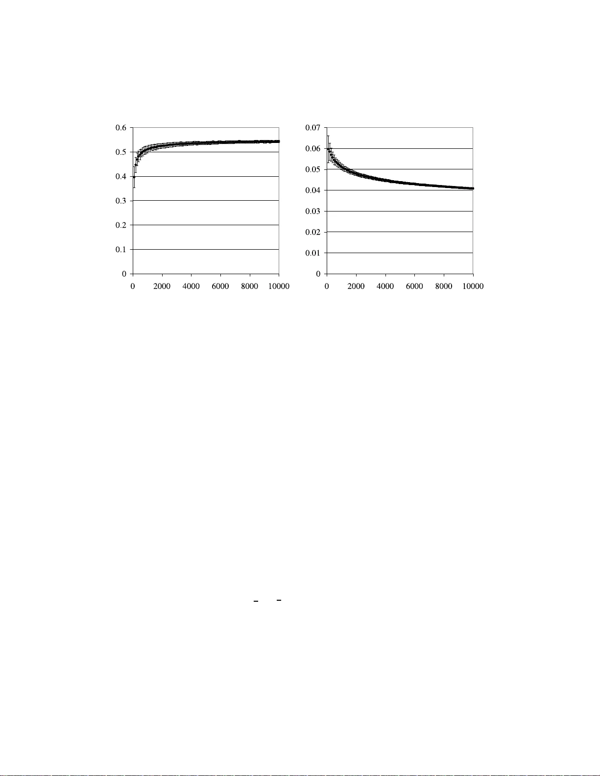
Av erage-Case Analysis of Online T op ological Ordering ∗ Deepak Ajwani † T obias F riedric h † Abstract Man y applications lik e p oin ter analysis and increme n tal compi- lation require main ta ining a topolo gical ordering of the no des of a directed acyclic gra ph (D A G ) under dynamic up dat es. All kno wn algorithms for this pro blem are either only analyzed for w o r st- case insertion sequences or only ev aluated exp erimen tally on random D A G s. W e presen t the first av erage-case analysis of online top ological ordering algorithms. W e prov e an exp ected run time of O ( n 2 p olylog ( n )) under insertion of the edges of a complete D A G in a random order for the algorit hms of Alp ern et al. (SODA, 1 990), Ka triel and Bo dlaender (T ALG, 2 006), and P earce and Kelly (JEA, 200 6). This is muc h less tha n the b est kno wn w orst-case b ound O ( n 2 . 75 ) for this problem. 1 In tr o ducti on There has been a grow ing in terest in dynamic graph algorithms o v er t he last tw o decades due to their a pplicatio ns in a v ariety of con texts includ- ing op erating systems, information systems, net w ork managemen t, assem bly planning, VLSI design and graphical applications. Ty pical dynamic graph algorithms maintain a certain prop ert y (e. g., connectivity information) of a graph that c hanges (a new edge inserted o r a n existing edge deleted) dy- namically ov er time. An alg orithm or a problem is called ful ly dynami c if ∗ A confere nce version appear ed in the 1 8th Int ernationa l Sy mposium on Algor ithms and Computation (ISAA C 200 7). † Max-Planck-Institut f¨ ur Infor matik, Saarbr ¨ uc ken, Germany 1 1 INTR OD UCTION 2 b oth edge insertions and deletions are allow ed, and it is called p artial ly dy- namic if o nly one (either only insertion or only deletion) is allow ed. If only insertions are a llo wed, the partially dynamic algorithm is called incremen- tal; if only deletions are a llo wed, it is called decremen tal. While a n um b er of fully dynamic algo rithms hav e b een obtained for v arious prop erties on undirected gr aphs (see [10] and references therein), the design a nd analy- sis of fully dynamic algorithms for directed gra phs has turned out to b e m uc h ha r der (e. g., [13, 24–26]). Muc h of the researc h on directed graphs is therefore concen tra t ed on the design o f partially dynamic algorithms in- stead (e. g., [3, 7, 14]). In this pap er, w e fo cus on the ana lysis of algorithms for maintaining a top ological ordering o f directed graphs in an incremen tal setting. A top ological order T of a directed graph G = ( V , E ) (with n := | V | and m := | E | ) is a linear ordering of its no des suc h that for all directed paths from x ∈ V to y ∈ V ( x 6 = y ), it holds that T ( x ) < T ( y ). A directed graph has a top o lo gical o rdering if and only if it is a cyclic. There are we ll-kno wn algorithms for computing the top ological o rdering of a directed acyclic graph (D A G) in O ( m + n ) time in an offline setting (see e. g . [8]). In a fully dynamic setting, eac h time an edge is added or deleted from the D A G , w e are required to up date the bijectiv e mapping T . In the o nline/incremen tal v arian t of this problem, the edges o f the DA G are not kno wn in adv ance but a r e inserted one at a time (no deletions allow ed). As the top ological order r emains v alid when remo ving edges, most algorithms fo r online top o logical ordering can also handle the fully dynamic setting. How ev er, there are no g o o d b ounds kno wn fo r the fully dynamic case. Most algorit hms are only analyzed in the online setting. Giv en an arbitr a ry sequence of edges, the online cycle detection problem is to disco v er t he first edge which intro duces a cycle. Till no w, the b est kno wn algorithm for this problem inv olv es main ta ining an online top olo g ical order and returning the edge after which no v alid top olo gical order exists. Hence, results for online top ological ordering also translate into results for the online cycle detection problem. Online top o logical ordering is required for incremen tal ev aluation o f computational circuits [2] and in incremen tal compilation [16, 18] where a dep endency graph b etw een mo dules is main- tained to r educe the amount of recompilation p erformed when an up date o ccurs. An application f or online cycle detection is p oin t er analysis [21]. F o r inserting m edges, the na ¨ ıv e wa y of computing an online top ologi- cal order eac h time from scratc h with the offline alg orithm t ak es O ( m 2 + 1 INTR OD UCTION 3 mn ) time. Marc hetti- Spaccamela, Nanni, and Rohnert [17] gav e an algo- rithm that can insert m edges in O ( mn ) time. Alp ern, Ho ov er, Rosen, Sw eeney , and Za dec k (AHRSZ) prop osed an algorithm [2] whic h runs in O ( |i ˆ K h| log ( |i ˆ K h| )) time p er edge insertion with |i ˆ K h| b eing a lo cal mea- sure of the insertion complexit y . Ho we v er, there is no analysis o f AHRSZ for a sequence of edge insertions. Katriel and Bo dlaender (KB) [14] an- alyzed a v arian t of the AHRSZ algorithm and obtained an upp er b ound of O (min { m 3 2 log n, m 3 2 + n 2 log n } ) for inserting an arbitrary sequence of m edges. The algorithm b y P ear ce and Kelly (PK) [19] empirically o ut p erfo rms the other algor it hms for random edge insertions leading to sparse random D A Gs, alt ho ugh its worst-case runtime is inferior to KB. Ajwani, F riedric h, and Mey er (AFM) [1] prop o sed a new algorithm with run t ime O ( n 2 . 75 ), whic h asymptotically outp erforms KB on dense DA Gs. As noted ab o v e, the empirical p erformance on random edge insertion sequence s ( R EIS) for the ab ov e algor it hms are quite differen t from their w o r st- cases. While PK p erforms empirically b etter for REIS, KB and AFM are the b est known algo r ithms fo r w orst-case sequence s. This leads us to the theoretical study of online t o p ological ordering algorithms on REIS. A nice prop ert y o f suc h an av erage-case analysis is that (in contrast to w orst-case b ounds) the av erage of exp erimen t a l results on REIS conv erge tow ards the real a v erage after sufficien tly man y iteratio ns. This can giv e a go o d indication of the tigh tness of the pro v en theoretical b ounds. Our con tributions are as follows : • W e sho w an expected runtime of O ( n 2 log 2 n ) for inserting all edges of a complete D A G in a random order with PK (cf. Section 4). • F or AHRSZ and KB, w e sho w an expected run time of O ( n 2 log 3 n ) for complete random edge insertion sequences (cf. Section 5). This is significan tly b etter tha n the kno wn w o rst-case b o und o f O ( n 3 ) f or KB to insert Ω( n 2 ) edges. • Additionally , w e sho w that f or suc h edge insertion sequences, the ex- p ected n um b er of edges which force an y algorithm to c hange the to p o- logical order (“ in v alidating edges”) is O ( n 3 2 √ log n ) (cf. Section 6 ), whic h is the first suc h result. The remainder of this pap er is organized as follows. The next section describes briefly the three algorithms AHRSZ, K B, and PK. In Section 3 we 2 ALGORITHMS 4 sp ecify the random g r a ph mo dels used in our analysis. Sections 4-6 pro v e our upp er b ounds for the run time of the three algorithms and the num b er of in v alidating edges. Section 7 presen ts an empirical study , whic h pro vides a deep er insigh t on the a v erage case b eha vior of AHRSZ and PK. 2 Algorith ms This section first in tro duces some notat io ns and then describ es the three algorithms AHRSZ, KB, a nd PK. W e keep the curren t top olo gical o rder as a bijectiv e function T : V → [1 ..n ]. In this and the subseque n t sections, w e will use the follo wing notations: d ( u, v ) denotes | T ( u ) − T ( v ) | , u < v is a short form of T ( u ) < T ( v ) , u → v denotes an edge from u to v , and u v expresse s t ha t v is reac hable from u . Note that u u , but not u → u . The de gr e e of a no de is the sum of its in- and out-degree. Consider the i -th edge insertion u → v . W e say tha t an edge insertion is invalidating if u > v b efore the insertion of this edge. W e define R ( i ) B := { x ∈ V | v ≤ x ∧ x u } , R ( i ) F := { y ∈ V | y ≤ u ∧ v y } and δ ( i ) = R ( i ) F ∪ R ( i ) B . Let | δ ( i ) | denote the n um b er of no des in δ ( i ) and let k δ ( i ) k denote the n umber of edges inciden t to no des of δ ( i ) . Note that δ ( i ) as defined ab ov e is differen t from the ada ptiv e parameter δ of the b ounded incremen tal computation mo del. If an edge is non-in v alidating , then | R ( i ) B | = | R ( i ) F | = | δ ( i ) | = 0. Note that for an in v alidating edge, R ( i ) F ∩ R ( i ) B = ∅ as ot herwise the algo rithms will just rep ort a cycle and terminate. W e now describ e the insertion of the i -th edge u → v fo r all the thr ee algorithms. Assume for the remainder o f this section that u → v is an in v alidating edge, as otherwise none of the algorithms do an ything for that edge. W e define an alg o rithm to b e lo c al if it only c hanges the ordering of no des x with v ≤ x ≤ u to compute the new top ological order T ′ of G ∪ { ( u, v ) } . All three algorithms are lo cal and they w ork in t w o phases – a “disco very phase” and a “relab elling phase”. In the disco v ery phase of PK , the set δ ( i ) is identified using a forward depth-first searc h from v (giving a set R ( i ) F ) and a bac kward depth- first searc h from u (giving a set R ( i ) B ). The relab elling phase is also v ery simple. It sorts b oth sets R ( i ) F and R ( i ) B separately in increasing top ological or der and t hen allo cates new priorities according to the relativ e p osition in the sequence R ( i ) B follo w ed b y R ( i ) F . It do es not alter the priority of an y no de not in δ ( i ) , thereb y 2 ALGORITHMS 5 greatly simplifying the relab eling phase. The run time of PK for a single edge insertion is Θ( k δ ( i ) k + | δ ( i ) | lo g | δ ( i ) | ). Alp ern et al. [2] used the b ounded incremen tal computation mo del [24] and in tro duced the measure | i ˆ K h| . F or an in v alidated top olog ical order T , the set K ⊆ V is a c o ver if for all x, y ∈ V : ( x y ∧ y < x ⇒ x ∈ K ∨ y ∈ K ). This states that for any connected x and y whic h are incorrectly ordered, a cov er K m ust include x or y or b oth. | K | and k K k denote the n um b er of no des and edges touc hing no des in K , resp ectiv ely . W e define |i K h| := | K | + k K k and a cov er ˆ K to b e minim al if |i ˆ K h| ≤ | i K h| for any other co v er K . Th us, |i ˆ K h| captures the minimal amoun t of work required to calculate the new top ological order T ′ of G ∪ { ( u, v ) } assuming that the algorithm is lo cal and that the adjacen t edges m ust b e tra v ersed. AHRSZ s disc ove ry phase marks the no des of a co v er K by marking some of the unmarke d no des x, y ∈ δ ( i ) with x y a nd y < x . This is done recursiv ely b y moving tw o fron tiers starting from v a nd u to w a r ds eac h other. Here, the crucial decision is whic h frontier to mo v e next. AHRSZ tries to minimize k K k b y balancing the n um b er of edges seen on b oth sides of the fron tier. The recursion stops when forward and ba ckw ard f ron tier meet. No t e that w e do not necessarily visit all no des in R ( i ) F ( R ( i ) B ) while extending the forw ard frontie r ( ba ckw ard f ron t ier). It can b e prov en [2] that the ma r ked no des indeed form a co v er K and that |i K h| ≤ 3 |i ˆ K h| . The r elab e l i n g phase emplo ys the dynamic prio rit y space data structure due to Dietz and Sleator [9]. This p ermits new priorities to b e created b e- t w een existing ones in O (1) amortized time. This is done in tw o passes ov er the no des in K . During the first pass, it visits the no des of K in rev erse top ological order and computes a strict upp er b ound on the new priorities to b e assigned to eac h no de. In the second phase, it visits the no des in K in top ological order and computes a strict low er b ound o n t he new priorit ies. Both together allow to assign new priorities to each no de in K . Thereafter they minimize t he n um b er of different lab els used to sp eed up the op era- tions on the prior ity space data structure in practice. It can b e prov en that the discov ery phase with |i ˆ K h| priority queue o p erations dominates the time complexit y , giving an o v erall b ound of O ( |i ˆ K h| log |i ˆ K h| ). KB is a slight mo dification of AHRSZ . In the disco very phase AHRSZ coun t s the total num b er of edges inciden t on a no de. KB coun ts instead only the in-degree of the backw ard frontie r no des and only the out-degree of the fo rw ard frontie r no des. In additio n, KB a lso simplified the relab eling phase. The no des visited during the extension of the for ward (back w ard) 3 RANDOM GRAPH MODEL 6 fron tier are deleted from the dynamic priorit y space data-structure and are reinserted, in the same relative o rder among themselv es, after (b efor e) all no des in R ( i ) B ( R ( i ) F ) not visited during the bac kw ar d (f o rw ard) frontier exten- sion. The alg o rithm th us computes a co v er K ⊆ δ ( i ) and its complexit y p er edge insertion is O ( |i K h| log |i K h| ). The worst case running time of KB fo r a sequen ce o f m edge insertions is O (min { m 3 2 log n, m 3 2 + n 2 log n } ). 3 Random Graph Mo del Erd˝ os and R ´ en yi [11, 12] introduced and p o pula r ized random graphs. They defined tw o closely related mo dels: G ( n, p ) and G ( n, M ). The G ( n, p ) mo del (0 < p < 1) consists of a gra ph with n no des in whic h each edge is c hosen indep enden tly with probability p . On t he o ther hand, the G ( n, M ) mo del assigns equal probability to a ll gra phs with n no des a nd exactly M edges. Eac h suc h graph o ccurs with a probability of 1  N M  , where N :=  n 2  . F o r o ur study of online top olog ical ordering alg orithms, w e use the ran- dom DA G mo del of Barak and Erd˝ os [4 ]. They obtain a ra ndom DA G by directing the edges of an undirected random graph fro m low er to higher indexed vertice s. Dep ending o n the underlying random graph mo del, this defines the DA G ( n, p ) and DA G ( n, M ) mo del. W e will mainly w o r k on the DA G ( n, M ) mo del since it is b etter suited to describ e incremen tal addition of edges. The set of all DA Gs with n no des is denoted b y DA G n . F or a random v a riable f with probabilit y space DA G n , E M [ f ] and E p [ f ] denotes the ex- p ected v alue in the DA G ( n, M ) and DA G ( n, p ) mo del, resp ectiv ely . F or the remainder of this pap er, w e set E [ f ] := E M [ f ] and q := 1 − p . The follo wing theorem shows that in most in v estigations the mo dels DA G ( n, p ) and DA G ( n, M ) a re practically inte rc hangeable, provide d M is close to pN . Theorem 1. Given a function f : DA G n → [0 , a ] with a > 0 an d f ( G ) ≤ f ( H ) for al l G ⊆ H and functions p and M of n with 0 < p < 1 and M ∈ N . 1. If lim n →∞ pq N = lim n →∞ pN − M √ pq N = ∞ , then E M [ f ] ≤ E p [ f ] + o (1 ) . 2. If lim n →∞ pq N = lim n →∞ M − pN √ pq N = ∞ , then E p [ f ] ≤ E M [ f ] + o (1 ) . 4 ANAL YSIS OF PK 7 The analogous theorem for the undirected gra ph mo dels G ( n, p ) and G ( n, M ) is we ll known . A closer lo o k at the pr o of for it giv en b y Bollo b´ as [6] rev eals that the proba bilistic argumen t used to sho w the close connection b et w een G ( n, p ) and G ( n, M ) can b e applied in the same manner for the t w o random D A G mo dels DA G ( n, p ) and DA G ( n, M ). W e define a random edge se quence to b e a uniform random permutation of the edges of a complete DA G , i. e., all p erm utations of  n 2  edges are equally lik ely . If the edges app ear to the o nline algorithm in the order in whic h they app ear in the random edge sequence, we call it a random edge insertion sequence (REIS). Note that a D A G obtained after inserting M edges of a REIS will ha v e the same probability distribution as DA G ( n, M ). T o simplify the pro ofs, w e first show our results in DA G ( n, p ) mo del a nd then transfer them in the DA G ( n, M ) mo del b y Theorem 1. 4 Analysis of PK When inserting the i -th edge u → v , PK only regar ds no des in δ ( i ) := { x ∈ V | v ≤ x ≤ u ∧ ( v x ∨ x u ) } with “ ≤ ” defined according to the curren t to p o logical order. As discussed in Section 2, PK p erforms O ( k δ ( i ) k + | δ ( i ) | log | δ ( i ) | ) o p erations fo r inserting the i -th edge. The in tuition behind the pro ofs in this section is that in the early phase of edge-insertions (the first O ( n log n ) edges), the graph is sparse and so only a f ew edges are t ra verse d during the D FS trav ersals. As the graph gro ws, few er and few er no des are visited in D F S trav ersals ( | δ ( i ) | is small) and so the total nu m b er of edges tra v ersed in DFS tra v ersals (b ounded ab ov e b y k δ ( i ) k ) is still small. Theorems 4 and 10 of this section show for a random edge insertion sequence (REIS) of N edges that P N i =1 | δ ( i ) | = O ( n 2 ) and E h P N i =1 k δ ( i ) k i = O ( n 2 log 2 n ). This prov es the f o llo wing theorem. Theorem 2. F or a r a n dom e dge inse rtion se q uenc e (REI S ) le adi n g to a c omplete DA G, the exp e cte d runtime of PK is O ( n 2 log 2 n ) . A comparable pair (of no des) ar e t w o distinct no des x a nd y suc h that either x y or y x . W e define a p otential function Φ i similar to Katriel and Bo dlaender [14]. Let Φ i b e the n umber of compar a ble pairs af t er the insertion of i edges. Clearly , ∆Φ i := Φ i − Φ i − 1 ≥ 0 for all 1 ≤ i ≤ M , Φ 0 = 0, and Φ M ≤ n ( n − 1) / 2. (1) 4 ANAL YSIS OF PK 8 Theorem 3. F or al l e dge se quenc es, ( i ) | δ ( i ) | ≤ ∆Φ i + 1 and ( i i ) | δ ( i ) | ≤ 2∆Φ i . Pr o of. Consider the i -th edge ( u, v ). If u < v , the theorem is tr ivial since | δ ( i ) | = 0. Otherwise , eac h v ertex o f R ( i ) F and R ( i ) B (as defined in Sec- tion 2) g ets newly or dered with resp ect to u and v , resp ectiv ely . The set S x ∈ R ( i ) B ( x, v ) ∩ S x ∈ R ( i ) F ( u, x ) = { ( u , v ) } . This means that o v erall at least | R ( i ) F | + | R ( i ) B | − 1 no de pairs get newly ordered: ∆Φ i ≥ | R ( i ) F | + | R ( i ) B | − 1 = | δ ( i ) | − 1 . Also, since in this case ∆Φ i ≥ 1, | δ ( i ) | ≤ 2∆Φ i . Theorem 4. F or al l e dge se quenc es, N X i =1 | δ ( i ) | ≤ n ( n − 1) = O ( n 2 ) . Pr o of. By Theorem 3 (i), w e get N X i =1 | δ ( i ) | ≤ N X i =1 (∆Φ i + 1) = Φ N + N ≤ n ( n − 1) / 2 + n ( n − 1) / 2 = n ( n − 1) . The remainder of this section pro vides t he necessary to ols step by step to finally prov e the desired b o und on P N i =1 k δ ( i ) k in Theorem 10 . One can also in terpret Φ i as a random v aria ble in DA G ( n, M ) with M = i . The corresp onding function Ψ fo r DA G ( n, p ) is defined as the tota l num b er of comparable no de pairs in DAG ( n, p ). Pittel and T ungol [22] sho w ed the follo wing theorem. Theorem 5. F or p := c log ( n ) /n and c > 1 , E p [Ψ] = (1 + o (1 )) n 2 2  1 − 1 c  2 . Using Theorem 1 , this result can b e transformed to Φ as defined ab o v e for DA G ( n, M ) and giv es the follow ing b ounds for E M [Φ k ]. Theorem 6. F or n log n < k ≤ N − 2 n lo g n , E M [Φ k ] = (1 + o (1)) n 2 2  1 − ( n − 1) log n 2( k + n log n )  2 . F or N − 2 n log n < k ≤ N − 2 log n , E M [Φ k ] = (1 + o (1)) n 2 2 1 − ( n − 1) log n 2( k + p log n ( N − k ) ) ! 2 . 4 ANAL YSIS OF PK 9 Pr o of. The function Ψ : DAG n → [0 , N ] and Ψ ( G ) ≤ Ψ( H ) wherev er G ⊆ H . The later inequalit y is true as the no des a lready ordered in G will still remain ordered in H . F or n log n < k ≤ N − 2 n log n , consider p := k + n log n N . Then lim n →∞ pq N ≥ lim n →∞ log n n log n n N ≥ lim n →∞ ( n − 1) log 2 n 2 n = ∞ and lim n →∞ pN − k √ pq N ≥ lim n →∞ pN − k √ N ≥ lim n →∞ n log n √ N ≥ lim n →∞ n log n n ≥ lim n →∞ log n = ∞ . Since all the conditions of Theorem 1 are satisfied for t hese v alues of k and p , E M [Ψ] = O ( E p [Ψ]). In particular, E M [Φ k ] = E p =( k + n log n ) / N [Ψ] + o (1 ) = (1 + o (1)) n 2 2  1 − ( n − 1) log n 2( k + n log n )  2 . F o r N − 2 n log n < k ≤ N − 2 log n , w e choose p := k + √ log n ( N − k ) N . Clearly , p ≥ N − 2 n log n + p log n ( N − ( N − 2 log n )) N ≥ N − 2 n lo g n + √ 2 log n N . Using this, w e get lim n →∞ pq N ≥ lim n →∞ ( N − 2 n log n + √ 2 log n ) N ( N − k − p log n ( N − k )) N N . Observ e that f ( k ) := N − k − p log n ( N − k ) has it s minim um at k 0 = N − log ( n ) / 4 since f ′ ( k 0 ) = 0 and f ′′ ( k 0 ) = 2 / log n > 0 . Hence, w e conclude that f ( k ) is monot o nically decreasing in our interv al ( N − 2 n log n, N − 2 log n ) and att a ins its minim um at N − 2 log n . Therefore, N − k − p log n ( N − k ) ≥ 2 log n − √ 2 log n → ∞ , whic h in turn prov es lim n →∞ pq N = ∞ and lim n →∞ pN − k √ pq N ≥ lim n →∞ p log n ( N − k ) q N − k − p log n ( N − k ) ≥ lim n →∞ p log n = ∞ 4 ANAL YSIS OF PK 10 T ogether with Theorem 5, this yields E M [Φ k ] = E p =( k + √ log n ( N − k )) / N [Ψ] + o (1) = (1 + o (1)) n 2 2 1 − ( n − 1) log n 2( k + p log n ( N − k )) ! 2 . The degree sequence o f a random g raph is a w ell-studied problem. The follo wing theorem is sho wn in [6]. Theorem 7. I f pn/ log n → ∞ , then almost every gr aph G in the G ( n, p ) mo del satisfie s ∆( G ) = (1 + o (1 )) pn , wher e ∆( G ) is the maxim um de gr e e of a no de i n G . As noted in Section 3 , the undirected graph obtained by ig noring the directions of DA G ( n, p ) is a G ( n, p ) graph. Therefore, the ab ov e result is also true f o r the maxim um degree (in-degree + out-degree) of a no de in DAG ( n, p ). Using Theorem 1 , the ab ov e result can b e tra nsformed to DA G ( n, M ), as w ell. Theorem 8. With pr ob ability 1 − O ( 1 n ) , ther e is no no de with de gr e e higher than 21 M n for sufficien tly lar ge n and M > n log n i n DA G ( n, M ) . Pr o of. W e examine t he f o llo wing tw o functions: • f 1 ( g ) : Num b er of no des with degree at least g ( n ) • f 2 ( g ) := f 2 1 ( g ) F o r f 1 , f 2 in G ( n, p ), g ( n ) := pn + 2 √ pq n log n , and some constan t c , Bollob´ as [5] sho w ed E p [ f 1 ( g )] = O  1 n  , σ 2 p ( f 1 ( g )) = E p [ f 2 ( g )] − E 2 p [ f 1 ( g )] ≤ c · E p [ f 1 ( g )] . (2) Consider a n y random DA G ( n, M ). It mus t hav e b een obtained by taking a r a ndom g raph G ( n, M ) and ordering the edges. The degree of a no de in DA G ( n, M ) is the same a s the degree o f the corresp onding no de in G ( n, M ). W e break down the analysis dep ending on M . A t fir st, consider the simpler case of M >  ⌊ N n log n ⌋ − 2  n log n . The degree of an y no de in an 4 ANAL YSIS OF PK 11 undirected graph cannot b e higher than n − 1. How ev er, as M > N − 3 n log n , 21 · M n ≥ 21 2 ( n − 1) − 63 log n . F or sufficien tly large n this is gr eater than n − 1 and therefore, no no de can ha v e degree higher than it. Next, w e consider M ∈ ( k n lo g n, ( k + 1) n log n ] for 1 ≤ k < l , where l := ⌊ N n log n ⌋ − 2, and w e pro v e the theorem for eac h in terv al. W e choose p k := ( k + 2) n log n N , q k := 1 − p k , and g k ( n ) := p k n + 2 √ p k q k n log n and lo ok for the conditions in Theorem 1. Note tha t 0 < p k < 1, f 1 : G n → [0 , n ], f 2 : G n → [0 , n 2 ], and f i ( G ) ≤ f i ( H ) wherev er G ⊆ H for i = 1 , 2. The later inequalit y holds as the degree of a n y no de in H is greater tha n or equal to the corresp onding degree in G . F or 1 ≤ k < l , p k ≥ 3 n log n N ≥ 6 log n n − 1 and q k ≥ 1 −  N n log n  − 1  n log n N ≥ 1 −  N − n log n n log n  n log n N ≥ 2 log n n − 1 . So for eac h in terv al, lim n →∞ p k q k N ≥ lim n →∞ 6 log n n − 1 2 log n n − 1 N ≥ lim n →∞ 6 log 2 n = ∞ and b y M k ≤ ( k + 1) n log n and k + 2 ≤ ⌊ N n log n ⌋ , lim n →∞ pN − M √ pq N ≥ lim n →∞ pN − M √ pN ≥ lim n →∞ n log n p ( k + 2) n log n = lim n →∞ √ n log n √ k + 2 ≥ lim n →∞ n log n √ N ≥ lim n →∞ log n = ∞ In eac h interv al, all the conditions of Theorem 1 are satisfied and therefore, E M [ f i ( g k )] = E p k [ f i ( g k )] + o (1) for i = 1 , 2 a nd 1 ≤ k < l . Using Equa- tion (2), w e get E M [ f 1 ( g k )] = O ( E p k [ f 1 ( g k )]) = O  1 n  and σ 2 M ( f 1 ( g k )) = E M [ f 2 ( g k )] − E 2 M [ f 1 ( g k )] = O  E p k [ f 2 ( g k )] − E 2 p k [ f 1 ( g k )]  = O ( σ 2 p k ( f 1 ( g k ))) = O ( E p k [ f 1 ( g k )]) = O  1 n  . Therefore, b y substituting X := f 1 ( g k ), µ := E M [ f 1 ( g k )] = O  1 n  , σ 2 := σ 2 M ( f 1 ( g k )) = O  1 n  , and ν := 1 − µ in Cheb yshev’s inequality (Pr {| X − µ | ≥ 4 ANAL YSIS OF PK 12 ν } ≤ σ 2 ν 2 ), w e get Pr {| f 1 ( g k ) − µ | ≥ 1 − µ } ≤ O  1 n (1 − µ ) 2  = O  1 n  . Ho w ev er, Pr {| f 1 ( g k ) − µ | ≥ 1 − µ } = Pr { ( f 1 ( g k ) ≥ 1) or ( f 1 ( g k ) ≤ 2 µ − 1) } and since, µ = O  1 n  and f 1 ( g k ) is non-negative random v ariable, Pr { f 1 ( g k ) ≤ 2 µ − 1 } = 0 f o r sufficien tly larg e n . Therefore, Pr { f 1 ( g k ) ≥ 1 } = Pr {| f 1 ( g k ) − µ | ≥ 1 − µ } = O  1 n  . In other w ords, with proba bilit y (1 − O ( 1 n )), there is no no de with a degree higher than g k in any in terv a l. Ho w ev er, b y p k ≥ log n n w e g et g k ( n ) = p k n + 2 p p k q k n log n ≤ 3 p k n ≤ 6( k + 2) n log n n − 1 F o r sufficien tly larg e n , n n − 1 ≤ 7 6 , and this implies g k ( n ) ≤ 7 ( k + 2) lo g n ≤ 7( k + 2) k M n ≤ 21 M n . Therefore, with probability 1 − O ( 1 n ), there is no no de with a degree higher than 21 M n in G ( n, M ) and b y the argumen t ab ov e, in DA G ( n, M ). As the maximum degree of a no de in DAG ( n, i ) is O ( i/n ), w e finally just need t o sho w a b o und on P i ( i · | δ ( i ) | ) to prov e Theorem 10. This is do ne in the follo wing theorem. Theorem 9. F or DA G ( n, M ) and r := N − 2 log n , E " r X i =1 ( i · | δ ( i ) | ) # = O ( n 3 log 2 n ) . Pr o of. Let us decomp ose the analysis in three ste ps. First, we sho w a b ound on the first n lo g n edges. By definition of δ ( i ) , | δ ( i ) | ≤ n . Therefore, n log n X i =1 i · E  | δ ( i ) |  ≤ n log n X i =1 i · n = O  n 3 log 2 n  . (3) 4 ANAL YSIS OF PK 13 The second step is to b ound P t i = n log n i · | δ ( i ) | with t := N − 2 n log n . F or this, Theorem 3 (ii) sho ws for all k suc h that n log n < k < t that E " t X i = k | δ ( i ) | # ≤ 2 E " t X i = k ∆Φ i # = 2 E [Φ t − Φ k − 1 ] = 2 E [Φ t ] − 2 E [Φ k − 1 ] . (4) The function hidden in the o (1) in Theorem 5 is decreasing in p [22]. Hence, also the o (1) in The orem 6 is decreasing in k . Plugging this in Equation (4) yields (with s := n log n ) E " t X i = k | δ ( i ) | # ≤ (1 + o (1 )) n 2  1 − ( n − 1) log n 2( t + s )  2 −  1 − ( n − 1) log n 2( k − 1 + s )  2 ! = (1 + o (1)) n 2 ( n − 1) log n  2 2( k − 1 + s ) − 2 2( t + s ) + ( n − 1) log n 4  1 ( t + s ) 2 − 1 ( k − 1 + s ) 2  ≤ (1 + o (1 )) n 2 ( n − 1) log n  1 k − 1 + s − 1 t + s  ≤ (1 + o (1 )) n 2 ( n − 1) log n 1 k − 1 . (5) By linearit y of exp ectation and Equation (5), E " t X i = s +1 i | δ ( i ) | # = t X i = s +1  i E  | δ ( i ) |   ≤ log ( ⌈ t s ⌉ ) X j =1  2 j s 2 j s X i =2 ( j − 1) s +1 E  | δ ( i ) |   ≤ log ( ⌈ t s ⌉ ) X j =1  2 j s t X i =2 ( j − 1) s +1 E  | δ ( i ) |   ≤ log ( ⌈ t s ⌉ ) X j =1  2 j s (1 + o (1)) n 2 ( n − 1) log n 1 2 ( j − 1) s  = log ( ⌈ t s ⌉ ) X j =1  2(1 + o (1)) n 2 ( n − 1) log n  = 2(1 + o (1 ) ) n 2 ( n − 1) log 2 n = O ( n 3 log 2 n ) . 4 ANAL YSIS OF PK 14 F o r the last step consider a k suc h that t < k < r . Theorem 3 (ii) giv es E " r X i = k | δ ( i ) | # ≤ 2 E " r X i = k ∆Φ i # = 2 E [Φ r − Φ k − 1 ] = 2 E [Φ r ] − 2 E [Φ k − 1 ] . Using Theorem 6 and similar arguments as b efore, this yields (with s ( k ) := p log n ( N − k )) E " r X i = k | δ ( i ) | # ≤ (1 + o (1 )) n 2  1 − ( n − 1) log n 2( r + s ( r ))  2 −  1 − ( n − 1) log n 2( k − 1 + s ( k − 1))  2 ! = (1 + o (1)) n 2 ( n − 1) log n 2 2( k − 1 + s ( k − 1)) − 2 2( r + s ( r )) + ( n − 1) log n 4  1 ( r + s ( r )) 2 − 1 ( k − 1 + s ( k − 1 ) ) 2  ! . Since k + s ( k ) is monotonically increasing for t < k < r , 1 ( k + s ( k )) 2 is a monoton- ically decreasing function in this in terv al. Therefore, 1 ( r + s ( r )) 2 − 1 ( k − 1+ s ( k − 1)) 2 < 0, whic h pro v es the follow ing equation. E " r X i = k | δ ( i ) | # ≤ (1 + o (1 )) n 2 ( n − 1) log n  1 k − 1 + s ( k − 1) − 1 r + s ( r )  ≤ (1 + o (1 )) n 2 ( n − 1) log n 1 k − 1 . (6) By linearit y of exp ectation and Equation (6), E " r X i = N − 2 n l og n + 1 i | δ ( i ) | # = r X i = N − 2 n l og n + 1  i E  | δ ( i ) |   ≤ ( N − 2 lo g n ) r X i = N − 2 n log n +1 E  | δ ( i ) |  4 ANAL YSIS OF PK 15 ≤ ( N − 2 lo g n ) (1 + o (1)) n 2 ( n − 1) log n 1 N − 2 n lo g n − 1 = O ( n 3 log n ) . Theorem 10. F or DA G ( n, M ) , E " N X i =1 k δ ( i ) k # = O ( n 2 log 2 n ) . Pr o of. By definition of k δ ( i ) k , w e kno w k δ ( i ) k ≤ i a nd hence n log n X i =1 k δ ( i ) k = O ( n 2 log 2 n ) . Again, let r := N − 2 lo g n . Theorem 8 tells us that with probability greater than  1 − c ′ n  for some constan t c ′ , there is no no de with degree ≥ c i n (for c = 21). Since the degree of an arbitrary no de in a DA G is b ounded by n , w e g et with Theorems 4 and 9, E " r X i = n log n +1 k δ ( i ) k # = O E " r X i = n log n +1 c i | δ ( i ) | n # + E " r X i = n log n +1 n c ′ | δ ( i ) | n # ! = O  1 n E " r X i =1 ( i | δ ( i ) | ) # + n 2  = O  1 n  n 3 log 2 n  + n 2  = O ( n 2 log 2 n ) . By again using the fact that the degree of an arbitrary no de in a D AG is at most n , w e o btain E " N X i = r +1 k δ ( i ) k # = O  n · E " N X i = r +1 | δ ( i ) | #  = O  n · N X i = r +1 n  = O ( n 2 log n ) . Th us, E " N X i =1 k δ ( i ) k # = E " n log n X i =1 k δ ( i ) k # + E " r X i = n log n +1 k δ ( i ) k # + E " N X i = r +1 k δ ( i ) k # = O ( n 2 log 2 n ) + O ( n 2 log 2 n ) + O ( n 2 log n ) = O ( n 2 log 2 n ) . 5 ANAL YSIS OF AHRSZ AND KB 16 5 Analysis of AHRSZ and KB Katriel and Bo dlaender [14] in tro duced KB as a v ar ia n t of AHRSZ for whic h a w orst-case run time o f O (min { m 3 2 log n, m 3 2 + n 2 log n } ) can b e sho wn. In this section, w e pro v e an exp ected r un time of O ( n 2 log 3 n ) under random edge insertion sequences , b oth for AHRSZ and KB. Recall fr o m Section 2 that f or ev ery edge insertion there is a minimal co v er ˆ K ( i ) . The following theorem sho ws that δ ( i ) is also a v alid cov er in t his situation. Theorem 11. δ ( i ) is a valid c over. Pr o of. Consider the insertion of the i -t h edge ( u, v ) and consider a no de-pair x, y suc h that x y , but x > y . Since b efore the insertion of this edge, the t o p ological ordering was consisten t, x u → v y , x < u a nd v < y . T ogether with x > y , it implies x > v . No w x u and x ≥ v imply x ∈ δ ( i ) . Th us, for ev ery no de-pair ( x, y ) suc h that x y and x > y , x ∈ δ ( i ) and hence, δ ( i ) is a v alid co v er. Therefore, b y definition of |i ˆ K ( i ) h| , |i ˆ K ( i ) h| ≤ |i δ ( i ) h| = | δ ( i ) | + k δ ( i ) k . E " m X i =1 |i ˆ K ( i ) h| # ≤ m X i =1 | δ ( i ) | + E " m X i =1 k δ ( i ) k # = O ( n 2 log 2 n ) The la tter equality follow s from Theorems 4 a nd 10. The expected complexit y of AHRSZ on REIS is th us O  E h P m i =1 |i ˆ K ( i ) h| log n i  = O ( n 2 log 3 n ). KB a lso computes a cov er K ⊆ δ ( i ) and it s complexit y p er edge insertion is O ( |i K h| log |i K h| ). Therefore, |i K h| ≤ | δ ( i ) | + k δ ( i ) k and with a similar argumen t as ab ov e, the exp ected complexit y of K B on REIS is O ( n 2 log 3 n ). 6 Boundin g the n um b er of in v alidating e dges An interes ting question in all this analysis is ho w many edges will actually in v alidate the top ological ordering and force any algorithm to do something ab out them. He re, w e show a non- trivial upp er b ound on t he exp ected v a lue of the num b er of inv alidating edges on REIS. Consider the following random v aria ble: inv al ( i ) = 1 if the i -th edge inserted is an inv alidating edge; inv al ( i ) = 0 otherwise. 7 EMPIRICAL OBSER V A TIONS 17 Theorem 12. E " m X i =1 inv al ( i ) # = O (min { m, n 3 2 log 1 2 n } ) . Pr o of. If the i -th edge is inv alidating, | δ ( i ) | ≥ 2; otherwise inv al ( i ) = | δ ( i ) | = 0. In either case, inv al ( i ) ≤ | δ ( i ) | / 2. Thus , fo r s := n 3 2 log 1 2 n and t := min { m, N − 2 n log n } , E " t X i = s +1 inv al ( i ) # ≤ E " t X i = s +1 | δ ( i ) | 2 # ≤ (1 + o (1 )) n 2 ( n − 1) log n 2 s ≤ (1 + o (1)) 2 n 3 2 log 1 2 n. The second inequalit y fo llo ws by substituting k := s + 1 in Equation (5). Also, since the n um b er of inv alidating edges can b e at most equal to the total n um b er of edges, P s i =1 inv al ( i ) ≤ s . E " m X i =1 inv al ( i ) # = E " s X i =1 inv al ( i ) # + E " t X i = s +1 inv al ( i ) # + E " m X i = t inv al ( i ) # ≤ O ( s ) + O ( n 3 2 log 1 2 n ) + O ( n log n ) = O ( n 3 2 log 1 2 n ) . The second b ound E [ P m i =1 inv al ( i )] ≤ m is obvious b y definition of inv al ( i ). 7 Empirical obse rv ations In a ddition to the ac hiev ed a v erag e-case b o unds, we also examined AHRSZ and PK exp erimen tally using the implemen tation of David J. P ear ce [19] a v aila ble fro m www.mcs.vu w.ac.nz/ ˜ djp/dts.h tml. F or v arying num b er of v ertices n = 100 , 20 0 , . . . , 10 000, w e generated random edge insertion se- quences (R EIS) leading to complete DA Gs and av eraged the p erfo r mance parameter C ( n ) o v er 250 runs. The c hosen C ( n ) upp er b ounds the resp ec- tiv e r untimes. The p erformance parameter tak en for AHRSZ is C ( n ) := P i |i K h| log ( |i K h| ). W e kno w E [ C ( n )] = O ( n 2 log 3 n ) f rom Sec tion 5 and kno w that the o v erall runtim e is Ω( n 2 ) since the alg orithm has to insp ect a ll the edges b eing inserted. In our exp erimen tal setting, w e dis- co v ered t hat C ( n ) / ( n 2 log 2 n ) is apparen tly a decreasing f unction and that 7 EMPIRICAL OBSER V A TIONS 18 (a) C ( n )  ( n 2 log n ) (b) C ( n )  ( n 2 log 2 n ) Figure 1. Experimental results of AHRSZ for the insertion of the edges of a complete DA G in a random order. Th e hor izon tal axes describ e t he n um b er of v ertices n . The v ertical axes show the measured empiric al insertion costs C ( n ) := P i |i K h| log |i K h| relative t o (a) n 2 log n a nd (b) n 2 log 2 n , resp ectiv ely . The error bars sp ecify the sample standar d deviation. C ( n ) / ( n 2 log n ) is an increasing function. This empirical evidence suggests that C ( n ) is p ossibly b etw een Ω( n 2 log n ) and O ( n 2 log 2 n ). Figure 1 sho ws our experimental results for AHRSZ. W e consider C ( n ) := P i ( k δ ( i ) k + | δ ( i ) | lo g | δ ( i ) | ) as a p erformance param- eter for PK and o bserv e that C ( n ) /n 2 is decreasing while C ( n ) / ( n 2 log − 1 n ) is increasing. This indicates that C ( n ) = o ( n 2 ), whic h implies an actual run time of Θ( n 2 ) for PK on REIS since all Ω( n 2 ) edges ha v e t o b e insp ected. P earce and Kelly [19] show ed empirically that PK outp erforms AHRSZ o n sparse DA Gs. Our exp erimen ts extend this to dense DA Gs. Complemen ting Section 6, w e also examined empirically the n um b er of in- v a lidating edges fo r AHRSZ. The same experimental set-up as ab o v e suggests a quasilinear growth of P m i =1 inv al ( i ) b et w een Ω( n log n ) and O ( n lo g 2 n ). Note that the observ ed empirical b ound for AHRSZ is significantly low er than the general b ound O ( n 3 2 log 1 2 n ) of Theorem 12 whic h holds for all al- gorithms. 8 DISCUSSION 19 8 Discuss ion On random edge insertion sequenc es (REIS) leading to a complete DA G, w e ha v e sho wn an exp ected run time of O ( n 2 log 2 n ) fo r PK and O ( n 2 log 3 n ) for AHRSZ and KB while the trivial lo w er b ound is Ω( n 2 ). Extending the av erage case analysis for t he case where w e only insert m edges with m ≪ n 2 still remains op en. On the other hand, the only non-trivial lo w er b ound for this problem is by Ramalingam and Reps [23], who ha v e sho wn that an adve rsary can force any algorithm whic h main ta ins ex- plicit la b els to r equire Ω( n log n ) time complexity f o r inserting n − 1 edges. There is still a large gap b et wee n the low er b o und of Ω(max { n log n, m } ), the b est a v erag e-case b ound of O ( n 2 log 2 n ) and the w orst-case b ound of O (min { m 1 . 5 + n 2 log n, m 1 . 5 log n, n 2 . 75 } ). Bridging this gap remains an op en problem. Ac knowledgemen ts The authors are grateful to T elik epalli Ka vitha, Irit Katriel, and Ulric h Mey er for v a rious helpful discuss ions. References [1] D . Ajw ani, T. F riedric h, and U. Mey er. An O ( n 2 . 75 ) algorithm for online top ological o rdering. In Pr o c e e dings of the Sc andin avian Worksh op on A lgorithm The ory (SW A T ’06) , V ol. 405 9 of L e c tur e Notes in Computer Scienc e , pp. 53–64 , 200 6 . [2] B. Alp ern, R. Ho o v er, B. K. Rosen, P . F. Sw eeney , and F. K . Zadec k. Incremen tal ev aluat io n of computational circuits. In Pr o c e e dings of the A CM-SIAM Symp osium on Discr ete Algorithms (SODA ’90) , pp. 32–42, 1990. [3] G . Ausiello, G. F. Italiano, A. Marche tti-Spaccamela, a nd U. Nanni. Incremen tal a lgorithms for minimal length paths. J. Algorithms , 12 : 615–638, 1991. REFERENCES 20 [4] A. B. Bara k and P . Erd˝ os. On the maximal num b er of strongly inde- p enden t v ertices in a random a cyclic directed graph. SIAM Journal on A lgebr aic and D iscr ete Metho ds , 5:508–514, 1984. [5] B. Bollob´ a s. D egree sequences of random graphs. Di scr e te Math. , 33: 1–19, 1981. [6] B. Bollob´ as. R andom Gr ap h s . Cam bridge Univ. Press, 2001. [7] S. Cicerone, D . F rigio ni, U. Nanni, and F. Pugliese. A uniform approach to semi-dynamic problems on digra phs. The or. Comput. Sci. , 203:69 – 90, 1998. [8] T. Cormen, C. Leiserson, and R. Riv est. Intr o duction to Algorithms . The MIT Press, Cam bridge, MA, 1989. [9] P . F. Dietz a nd D. D. Sleator. Tw o algorithms for maintaining order in a list. In Pr o c e e dings of the ACM Symp osium on The ory of Computing (STOC ’87) , pp. 365–372, 1987. [10] D. Eppstein, Z. Galil, and G. F. Italiano. Dynamic g r a ph alg orithms. In M. J. Atallah, editor, A lgorithms an d The ory of Com putation Handb o ok , c ha pt er 8. CR C Press, 1999. [11] P . Erd˝ os and A. R´ en yi. O n rando m gr a phs. Publ Math D ebr e c en , 6: 290–297, 1959. [12] P . Erd˝ os and A. R´ eny i. On the ev olution o f rando m graphs. Magyar T ud. Akad. Mat. K utato Int. Kozl. , 5:17 – 61, 1 9 60. [13] D. F rigioni, A. Marchetti-Spaccamela, and U. Nanni. F ully dynamic shortest paths and negativ e cycles detection on digraphs with a rbitrary arc w eights. In Pr o c e e d ings of the Eur o p e an Symp osium on Algorithms (ESA ’98) , V ol. 1461 of L e ctur e Notes in Computer Scie nc e , pp. 320–331, 1998. [14] I. Katriel and H. L. Bo dlaender. Online top olog ical ordering. A CM T r ans. Algorithms , 2:364– 3 79, 2006. Preliminary version app eared as [15]. REFERENCES 21 [15] I. Katriel and H. L. Bodla ender. Online top o logical ordering. In Pr o c e e d- ings of the A CM-SIAM Symp osium on D iscr ete A lgorithms (SODA ’05) , pp. 443–450 , 2005. [16] A. Marc hetti-Spaccamela, U. Nanni, and H. Rohnert. On-line g r a ph algorithms for incremen tal compilation. In Pr o c e e di n gs of the Workshop on Gr aph-Th e or etic Con c epts in Computer Scienc e (WG ’ 9 3) , V ol. 7 90 of L e ctur e Notes in Computer Scienc e , pp. 70–86, 1993. [17] A. Marchetti-Spaccamela, U. Nanni, and H. Rohnert. Main taining a top ological order under edge insertions. Information Pr o c e s s ing L etters , 59:53–58, 1996. [18] S. M. Omohundro, C.-C. Lim, and J. Bilmes. The sather la nguage com- piler/debugger implemen tation. T ec hnical Rep ort 92-017 , In ternationa l Computer Science Institute, Berk eley , 1992. [19] D. J. P earce and P . H. J. Kelly . A dynamic top ological sort algorithm for directed a cyclic g raphs. J. Ex p . Algorithmics , 11:1.7 , 2006. Preliminary v ersion app eared as [20]. [20] D. J. Pearce and P . H. J. Kelly . A dynamic algorithm fo r top ologically sorting directed a cyclic graphs. In Pr o c e e dings of the Workshop on Ex- p erimental and Efficient Algorithms (WEA ’04) , V ol. 3 059 of L e ctur e Notes in Computer Scienc e , pp. 383–398, 2004. [21] D. J. P earce, P . H. J. Kelly , and C. Hankin. Online cycle detection and difference pro pagation: Applications to p oin ter a na lysis. S oftwar e Quality Journal , 12:311–33 7 , 200 4 . [22] B. Pittel and R. T ungol. A phase tra nsition phenomenon in a random directed acyclic graph. R andom Struct. A lgorithms , 18:164–1 8 4, 2001. [23] G. Ramalingam and T. W. Reps. On comp etitive on-line algorithms for the dynamic priorit y-o rdering problem. In formation Pr o c essing L etters , 51:155–16 1, 19 9 4. [24] G. Ra malingam and T. W. Reps. On the computational complexit y of dynamic graph problems. The or. Comput. Sci. , 158:233– 2 77, 1996. REFERENCES 22 [25] L. Ro ditt y and U. Zwick . A f ully dynamic reac habilit y algorithm for directed gra phs with an almost linear up date time. In Pr o c e e dings of the ACM Symp osium o n The ory of C o mputing (STOC ’ 0 4) , pp. 18 4– 191, 2004. [26] L. R o ditt y a nd U. Zwic k. O n dynamic shortest paths problems. In Pr o c e e d ings of the Eur op e an S ymp osium on Algorithms (ESA ’04) , V ol. 3221 of L e c tur e Notes in Computer Scienc e , pp. 580–591. Springer, 2004.