Some thoughts on the asymptotics of the deconvolution kernel density estimator

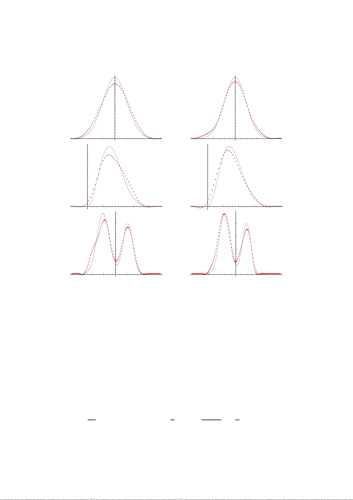
Some though ts on the asymptotics of t he decon v olution k ernel densit y estima tor Bert v an Es Kortew eg-de V ries Instituut voor Wiskunde Univ ersiteit v an Amsterdam Plan tage Muid ergrac h t 24 1018 TV Amsterdam The Netherlands v anes@ s cience.uv a.nl Shota Gugush vili ∗ Eurandom T ec hnisc he Univ ersiteit Eind ho ve n P .O. Bo x 513 5600 MB Eindho ven The Netherlands gugush vili@eur an d om.tue.nl No v em b er 12, 2018 Abstract Via a sim ulation study we compare the finite sample perfo r mance of the deconv olution k ernel density estimator in the sup ersmo oth deco n- volution pr o blem to its asymptotic behaviour predicted b y tw o asymp- totic normality theorems. Our results indicate that for lo wer noise levels and mo der a te sample sizes the matc h betw een the asympto tic theory and the finite sa mple p erfo r mance of the estimator is not satis- factory . On the other hand we show that the tw o appro aches pr o duce reasona bly clo se r esults for higher noise levels. T hes e observ ations in turn provide additional motiv ation for the study of dec o nv olution prob- lems under the assumption that the erro r term v ariance σ 2 → 0 as the sample size n → ∞ . Keywords: finite sample behavior, asymptotic normality , deco nv olu- tion kernel density estimator , F ast F ourier T ransfo rm. ∗ The research of this author w as financially supp orted b y the Nederlandse Organisatie voor W eten schapp elijk Onderzo ek (NWO). P art of the work wa s done while th is author w as at the Kortew eg-de V ries Instituut voor Wiskun de in Amsterdam. 1 AMS sub ject classifica tion: 62G07 2 1 In tro du ction Let X 1 , . . . , X n b e i.i.d. observ ations, where X i = Y i + Z i and the Y ’s and Z ’s are ind ep endent. Assume that the Y ’s are unobs er v able and that they ha v e the density f and also that the Z ’s ha ve a kno wn d ensit y k . The decon v olution prob lem consists in estimation of the densit y f based on the sample X 1 , . . . , X n . A p opular estimator of f is th e decon vo lution k ernel d ensit y estimator, whic h is constructed via F ourier in ve rs ion and k ernel smo othing. Let w b e a k ern el fu nction and h > 0 a b an d width. The k ern el decon vol ution density estimator f nh is defined as f nh ( x ) = 1 2 π Z ∞ −∞ e − itx φ w ( ht ) φ emp ( t ) φ k ( t ) dt = 1 nh n X j =1 w h  x − X j h  , (1) where φ emp denotes the empirical c haracteristic function of the sample, i.e. φ emp ( t ) = 1 n n X j =1 e itX j , φ w and φ k are F ourier transforms of the functions w and k , resp ectiv ely , and w h ( x ) = 1 2 π Z ∞ −∞ e − itx φ w ( t ) φ k ( t/h ) dt. The estimator (1) wa s pr op osed in Carroll and Hall (1988) and Stefanski and Carroll (1990) and there is a v ast amount of literature dedicated to it (for additional bibliographic information see e.g. v an Es and Uh (200 4 ) and v an Es and Uh (2005)). Dep ending on the rate of deca y of the c haracteristic fu nction φ k at plus and minus in finit y , decon v olution problems are usually divided in to tw o groups, ordinary sm o oth decon vo lution p roblems and sup ersm o oth decon v o- lution problems. In the first case it is assumed that φ k deca ys algebraically and in the second case the deca y is essentia lly exp onen tial. This r ate of deca y , and consequently the smo othness of the d ensit y k , has a decisiv e in- fluence on the p erformance of (1). T he general picture that one sees is th at smo other k is, th e harder th e estimatio n of f b ecomes, see e.g. F an (1991a). Asymptotic n ormalit y of (1 ) in the ordinary smo oth case was established in F an (1991 b ), see also F an and Liu (1997). The limit b eha viour in this case is essen tially the same as that of a k ernel estimator of a higher order deriv ativ e of a densit y . Th is is ob vious in certain relativ ely s im p le cases where the estimator is actually equal to the su m of deriv ativ es of a k ernel densit y estimator, cf. v an Es and Kok (1998). Our main interest, ho w ev er, lies in asymptotic normalit y of (1) in the sup ersmo oth case. In this case u n der certain conditions on the k ernel w and the u nknown densit y f , the f ollo wing theorem was p ro ve d in F an (1992). 3 Theorem 1.1. L et f nh b e define d by (1) . Then √ n s n ( f nh ( x ) − E [ f nh ( x )]) D → N (0 , 1) (2) as n → ∞ . Her e either s 2 n = (1 /n ) P n j =1 Z 2 nj , or s 2 n is the sample varianc e of Z n 1 , . . . , Z nn with Z nj = (1 /h ) w h (( x − X j ) /h ) . The asymptotic v ariance of f nh itself do es not follo w f rom this r esu lt. O n the other han d v an Es and Uh (2004), see also v an Es and Uh (2005), de- riv ed a cen tral limit theorem for (1) w here the normalisation is deterministic and the asymptotic v ariance is given. F or th e p urp oses of the present wo rk it is sufficien t to use the r esu lt of v an Es and Uh (2005). Ho w eve r, b efore recalling the corresp onding theo- rem, w e firs t formulate conditions on the kernel w and the d ensit y k . Condition 1.1. L et φ w b e r e al-v alue d, symmetric and have supp ort [ − 1 , 1] . L et φ w (0) = 1 , and assume φ w (1 − t ) = At α + o ( t α ) as t ↓ 0 for some c onstants A and α ≥ 0 . The simplest example of suc h a kernel is the sin c kernel w ( x ) = sin x π x . (3) Its c haracteristic fu n ction equals φ w ( t ) = 1 [ − 1 , 1] ( t ) . In this case A = 1 and α = 0 . Another k ernel satisfying Cond ition 1.1 is w ( x ) = 48 cos x π x 4  1 − 15 x 2  − 144 sin x π x 5  2 − 5 x 2  . (4) Its corresp onding F our ier transform is giv en by φ w ( t ) = (1 − t 2 ) 3 1 [ − 1 , 1] ( t ) . Here A = 8 an d α = 3 . Th e k ernel (4) was used for sim ulations in F an (1992) and its go o d p erf ormance in decon vo lution con text w as established in Delaig le and Hall (2006). Y et another example is w ( x ) = 3 8 π  sin( x/ 4) x/ 4  4 . (5) The corresp ondin g F our ier transform equals φ w ( t ) = 2(1 − | t | ) 3 1 [1 / 2 , 1] ( | t | ) + (6 | t | 3 − 6 t 2 + 1)1 [ − 1 / 2 , 1 / 2] ( t ) . Here A = 2 and α = 3 . This kernel w as considered in W and (1998) and Delaigl e and Hall (2006). No w we formulate the condition on the d ensit y k . 4 Condition 1.2. Assume that φ k ( t ) ∼ C | t | λ 0 exp  −| t | λ /µ  as | t | → ∞ , for some λ > 1 , µ > 0 , λ 0 and some c onstant C. F urthermor e, let φ k ( t ) 6 = 0 for al l t ∈ R . The follo wing theorem h olds tru e, see v an Es and Uh (2005). Theorem 1.2. Assume Conditions 1.1 and 1.2 and let E [ X 2 ] < ∞ . Then, as n → ∞ and h → 0 , √ n h λ (1+ α )+ λ 0 − 1 e 1 / ( µh λ ) ( f nh ( x ) − E [ f nh ( x )]) D → N  0 , A 2 2 π 2  µ λ  2+2 α (Γ( α + 1)) 2  . Her e Γ denotes the gamma function. The goal of the p resen t note is to compare the theoretical b eha viour of the estimator (1) p redicted by Th eorem 1.2 to its b eha viour in practice, whic h will b e done via a limited simulatio n study . T he obtained results can b e used to compare Theorem 1.1 to Theorem 1.2, e.g. whether it is preferable to u se the sample standard deviation s n in the construction of p oint w ise confidence interv als (computation of s n is more in volv ed) or to use the norm alisation of Theorem 1.2 (this in vo lves ev aluatio n of a simpler expression). The rest of the pap er is organised as follo ws: in Section 2 we present some s im ulation results, wh ile in S ection 3 we discuss th e obtained results and dra w conclusions. 2 Sim ulation results All the simulatio ns in this sectio n w ere done in Mathematica. W e considered three target densities. Th ese densities are: 1. dens ity # 1: Y ∼ N (0 , 1); 2. dens ity # 2: Y ∼ χ 2 (3); 3. dens ity # 3: Y ∼ 0 . 6 N ( − 2 , 1 ) + 0 . 4 N (2 , 0 . 8 2 ) . The densit y # 2 w as chosen b ecause it is s k ewe d, while the density # 3 w as selected b ecause it has t wo u n equal mo des. W e also assumed that th e noise term Z w as N (0 , 0 . 4 2 ) distribu ted. Notice that the n oise-to-sig nal ratio NSR = V ar[ Z ] / V ar [ Y ]100% for the d ensit y # 1 equals 16% , for the densit y # 2 it is equal to 2 . 66% , and f or the densit y # 3 it is giv en by 3% . W e hav e c hosen the sample size n = 50 and generated 500 samples from the density g = f ∗ k . Notice that su c h n w as also used in simulat ions in e.g. Delaig le and Gijb els (2004). Ev en though at the first sigh t n = 50 migh t lo ok to o small for normal decon vo lution, for th e lo w noise leve l that w e ha ve the deconv olution k ern el densit y estimator will still p erf orm well, cf. W and (19 98 ). As a k ernel we to ok the ke rn el (4). F or eac h mo d el 5 that we considered, the theoretically optimal b an d width, i.e. the b an d width minimising MISE[ f nh ] = E  Z ∞ −∞ ( f nh ( x ) − f ( x )) 2 dx  , (6) the mean-squared err or of the estimator f nh , was selected by ev aluating (6) for a grid of v alues of h k = 0 . 01 k , k = 1 , . . . , 100 , and selecting the h that minimised MISE[ f nh ] on that grid. Notice that it is easier to ev aluate (6) b y rewriting it in terms of the c haracteristic f u nctions, whic h can b e done via P arsev al’s identit y , cf. Stefanski and Carroll (1990). F or r eal data of course the ab o ve metho d d o es not w ork, b ecause (6) dep end s on the unknown f . W e refer to Delaigle and Gijb els (2004) for data-dep endent band width selection metho ds in ke rn el decon v olution. F ollo wing the r ecommendation of Delaigl e and Gijb els (2007), in order to av oid p ossible numerical issu es, the F ast F our ier T ran s form w as used to ev aluate the estimate (1) . Sev eral outcome s for tw o sample sizes, n = 50 and n = 100 , are giv en in Figure 1. W e see that the fit in general is quite reasonable. This is in line with resu lts in W and (1998), w here it w as sho wn b y finite samp le calculatio ns that the decon vol ution k ernel densit y estimator p erforms well ev en in the sup ersmo oth noise distribu tion case, if the noise lev el is not to o high. In Figure 2 w e provi d e histograms of estimates f nh ( x ) that we obtained from our sim ulations for x = 0 and x = 0 . 92 (the densities # 1 and # 2) and for x = 0 and x = 2 . 04 (the density # 3). F or the density # 1 p oin ts x = 0 and x = 0 . 92 were selected b ecause the first corresp onds to its mo d e, while the second comes from the region where the v alue of the d ensit y is mo derately h igh. Notice that x = 0 is a b ou n dary p oin t for the su pp ort of densit y # 2 and that the deriv ativ e of dens ity # 2 is infin ite there. F or the densit y # 3 the p oint x = 0 corresp onds to the region b et ween its tw o m o des, while x = 2 . 04 is close to where it h as one of its mo des. The histograms lo ok satisfactory and ind icate that the asymptotic n ormalit y is not an issu e. Our main in terest, ho wev er, is in comparison of the sample standard deviation of (1) at a fixed p oint x to th e theoretical s tandard deviation computed using Th eorem 1.2. This is of practical imp ortance e.g. for con- struction of confidence inte rv als. The theoretical standard d eviation can b e ev aluated as TSD = A Γ( α + 1) h λ + α + λ 0 − 1 e 1 / ( µh λ ) √ 2 nπ 2  µ λ  1+ α , up on noticing that in our case, i.e. wh en using ke rn el (4) and the error distribution N (0 , 0 . 4 2 ) , we ha ve A = 8 , α = 3 , λ 0 = 0 , λ = 2 , µ = 2 / 0 . 4 2 . After comparing this theoretical v alue to the samp le standard deviation of the estimator f nh at p oin ts x = 0 and x = 0 . 92 (the densities # 1 and # 2) 6 - 3 - 2 - 1 1 2 3 0.1 0.2 0.3 0.4 - 4 - 2 2 4 0.1 0.2 0.3 0.4 - 1 1 2 3 4 0.1 0.2 0.3 0.4 0.5 0.6 - 1 1 2 3 4 0.1 0.2 0.3 0.4 0.5 0.6 - 6 - 4 - 2 2 4 6 0.05 0.10 0.15 0.20 - 5 5 0.05 0.10 0.15 0.20 Figure 1: The estimate f nh (dotted line) and the true d ensit y f (thin line) for the dens ities # 1, # 2 and # 3. Th e left column giv es results for n = 50 , while the righ t column pr o vides results for n = 100 . and at p oint s x = 0 and x = 2 . 04 (the density # 3), see T able 1, w e notice a considerable discrep an cy (by a factor 10 for the densit y # 1 and ev en larger d iscrepancy for densities # 2 and # 3). A t th e same time the samp le means ev aluated at these t wo p oint s are close to the true v alues of the target densit y and b roadly corresp ond to the exp ected theoretical v alue f ∗ w h ( x ) . Note here that the bias of f nh ( x ) is equal to the bias of an ord inary kernel densit y estimator based on a sample fr om f , s ee e.g. F an (1991 a ). T o gain insigh t in to this striking discrepancy , recall h o w the asymptotic normalit y of f nh ( x ) w as deriv ed in v an Es and Uh (2 005 ). Adapting the pro of from th e latter pap er to our example, the firs t step is to rewr ite f nh ( x ) as 1 π h Z 1 0 φ w ( s ) exp[ s λ / ( µh λ )] ds 1 n n X j =1 cos  x − X j h  + 1 n n X j ˜ R n,j , (7) 7 0.25 0.3 0.35 0.4 0.45 10 20 30 40 50 0.15 0.2 0.25 0.3 0.35 10 20 30 40 50 0 0.05 0.1 0.15 0.2 10 20 30 40 50 60 0.2 0.3 0.4 0.5 0.6 10 20 30 40 50 60 0.025 0.05 0.075 0.1 0.125 0.15 10 20 30 40 0.05 0.1 0.15 0.2 0.25 0.3 10 20 30 40 50 Figure 2: T he h istograms of estimates f nh ( x ) for x = 0 and x = 0 . 92 f or the densit y # 1 (top t w o graphs), for x = 0 an d x = 0 . 92 for the densit y # 2 (mid dle t w o graphs), and for x = 0 and x = 2 . 04 for the densit y # 3 (b ottom t wo graph s). where the remainder terms ˜ R n,j are defin ed in v an Es and Uh (2 005 ). Then b y estimating the v ariance of the s econd summand in (7 ) , one can sho w that it can b e n eglecte d when consid er in g the asymp totic normalit y of (7) as n → ∞ and h → 0 . T ur ning to the first term in (7), one u ses the asymptotic equiv alence, cf. Lemma 5 in v an Es and Uh (2005), Z 1 0 φ w ( s ) exp[ s λ / ( µh λ )] ds ∼ A Γ( α + 1)  µ λ h λ  1+ α e 1 / ( µh λ ) , (8) whic h explains the shap e of th e normalising constant in Theorem 1.2. Ho w- ev er, this is precisely the p oin t whic h causes a large discrepancy b et we en the theoretical standard deviation and the sample stand ard deviation. Th e appro ximation is goo d asymptotically as h → 0 , bu t it is qu ite inaccurate 8 f h ˆ µ 1 ˆ µ 2 ˆ σ 1 ˆ σ 2 σ ˜ σ # 1 0.24 0.343 0.252 0.0423 0.039 0.429 0.072 # 2 0.18 0.066 0.389 0 .035 0.067 0.169 0.114 # 3 0.25 0.074 0.159 0.025 0. 037 0.512 0.068 T able 1: Sample means ˆ µ 1 and ˆ µ 2 and sample stand ard deviations ˆ σ 1 and ˆ σ 2 ev aluated at x = 0 and x = 0 . 92 (densities # 1 and # 2) and x = 0 and x = 2 . 04 (the d ensit y # 3) together with the theoretical standard deviation σ and the corrected theoretical standard d eviation ˜ σ . The bandwidth is giv en by h. for larger v alues of h. Indeed, consider the r atio of the left-hand side of (8) with the right-hand side. W e h av e plotted this ratio as a function of h for h r anging b et wee n 0 and 1 , see Figure 3. On e sees th at the r atio is close to 1 for extremely small v alues of h and is quite far from 1 for larger v alues of h. I t is equally easy to see that the p o or approximati on in (8) holds true for k ernels (3) and (5) as w ell, see e.g. Figure 3, wh ic h plots th e r atio of b oth sides of (8) for th e kernel (3 ). T his p o or approximat ion, of course, is n ot 0.2 0.4 0.6 0.8 1.0 0.5 1.0 1.5 0.2 0.4 0.6 0.8 1.0 0.4 0.6 0.8 1.0 1.2 Figure 3: Accuracy of (8) as a function of h for the kernels (4) (left figur e) and (3) (righ t figure). c haracteristic of only the p articular µ and λ that we us ed in our simulations, but also holds true for other v alues of µ and λ. Ob viously , one can correct f or the p o or appro ximation of the sample standard deviation by the theoretical standard deviation by using the left- hand side of (8) instead of its approxima tion. Th e theoretical standard deviation corrected in such a wa y is giv en in the last column of T able 1 . As it can b e seen from the table, this p ro cedur e led to an impro veme nt of the agreemen t b etw een th e th eoretical standard d eviation and its sample coun- terpart for all three target d ensities. Nev ertheless, the matc h is not en tirely satisfactory , since the corrected th eoretical stand ard deviation and the sam- ple standard deviation differ by factor 2 or eve n more. A p erfect matc h is imp ossible to obtain, b ecause we neglect the r emainder term in (7) and h is 9 still f airly large. W e further notice that the concurrence b et ween the results is b etter for x = 0 than for x = 0 . 92 for densities # 1 and # 2, and for x = 2 . 04 than for x = 0 for the d ensit y # 3. W e also p erformed simulat ions for the sample sizes n = 100 and n = 200 to chec k the effect of ha ving larger samples. F or brevity w e will rep ort only the r esults for densit y # 2, see Figure 4 and T able 2, since this dens it y is nontrivial to decon vol ve, though not as difficult as the dens it y # 3. Notice that th e results did not impro ve greatly for n = 100 , while for the case n = 200 the corrected theoretical standard deviation b ecame a w orse estimate of the sample standard devi- ation than the theoretical s tand ard d eviation. Explanati on of this cu rious phenomenon is giv en in Section 3. 0 0.025 0.05 0.075 0.1 0.125 0.15 10 20 30 40 0.25 0.3 0.35 0.4 0.45 0.5 0.55 10 20 30 40 0 0.02 0.04 0.06 0.08 0.1 0.12 10 20 30 40 0.3 0.35 0.4 0.45 0.5 0.55 10 20 30 40 Figure 4: T he h istograms of estimates f nh ( x ) for x = 0 and x = 0 . 92 f or the densit y # 2 for n = 100 (top t wo graphs) and for n = 200 (b ottom t wo graphs). n h ˆ µ 1 ˆ µ 2 ˆ σ 1 ˆ σ 2 σ ˜ σ # 100 0.17 0.063 0.393 0.025 0.051 0.108 0.090 # 200 0.15 0.052 0.402 0.023 0.049 0.070 0.084 T able 2: Sample means ˆ µ 1 and ˆ µ 2 and sample stand ard deviations ˆ σ 1 and ˆ σ 2 ev aluated at x = 0 and x = 0 . 92 for th e densit y # 2, together with the th eoretical standard d eviation σ and the corrected theoretical s tand ard deviation ˜ σ . 10 F urther m ore, note that V ar   1 √ n n X j =1 cos  x − X j h    → 1 2 as n → ∞ and h → 0 , see v an Es an d Uh (2005). This explains the ap- p earance of the factor 1 / 2 in the asymptotic v ariance in Th eorem 1.2. One migh t also qu estion the go o dn ess of this approximat ion and prop ose to use instead some estimator of V ar[cos(( x − X ) h − 1 )] , e.g. its empirical count er- part b ased on th e samp le X 1 , . . . , X n . Ho w ev er, in the simulat ions that we p erformed for all three target densities (with n and h as ab o v e), the result- ing estimates to ok v alues close to the tru e v alue 1 / 2 . E.g. for th e dens ity # 3 the samp le mean turned out to b e 0 . 502298 , while the sample standard deviation w as equal to 0 . 0535049 , thus sh o wing that th ere was insignificant v ariability around 1 / 2 in this particular example. On the other hand, for other distributions and for differen t sample s izes, it could b e the case th at the d irect use of 1 / 2 will lead to inaccurate results. Next w e rep ort some sim ulation results relev ant to Th eorem 1.1. This theorem tells us that for a fixed n w e ha ve that √ n s n ( f nh ( x ) − E [ f nh ( x )]) (9) is approximat ely normally distribu ted with zero mean an d v ariance equal to one. Up on using the fact th at E [ f nh ( x )] = f ∗ w h ( x ) , w e us ed the data th at w e obtained from our previous simulatio n examples to plot the histograms of (9) and to ev aluate the sample means and stand ard deviations, see Figure 5 and T able 3. One notices that the concurrence of the theoretical and sample v alues is quite go o d for th e densit y # 1. F or the density # 2 it is rather unsatisfactory for x = 0 , whic h is explainable by the fact th at in general there are very few obs er v ations originating from the neighbou r ho o d of this p oint. Finally , we notice that the matc h is reasonably go o d for the d ensit y # 3, giv en the fact that it is d ifficult to estimate, at the p oin t x = 2 . 04 , but is still u n satisfactory at the p oin t x = 0 . The latter is explainable by th e fact that there are less observ ations originating from the neigh b ourho o d of this p oint. An increase in the samp le size ( n = 100 and n = 200) leads to an impro vemen t of the matc h b etw een the theoretical and the sample mean and standard deviation at the p oin t x = 0 f or the densit y # 2, see Figure 6 and T able 4, ho wev er the results are still largely inaccurate for this p oin t. In essence similar conclusions w ere obtained for th e d ensit y # 3. These are not rep orted here. Note that in all three mo d els that we studied the noise lev el is not high. W e also stud ied the case when the noise level is v ery high. F or brevit y we present the results on ly f or the d ensit y # 1 and for sample size n = 50 . W e considered three cases of the error distribution: in th e fi r st 11 - 2 - 1 0 1 2 10 20 30 40 50 - 4 - 2 0 2 10 20 30 40 50 - 200 - 150 - 100 - 50 0 50 100 150 200 250 - 6 - 4 - 2 0 2 20 40 60 80 100 - 40 - 30 - 20 - 10 0 50 100 150 200 - 10 - 7.5 - 5 - 2.5 0 2.5 20 40 60 80 Figure 5: The h istograms of (9 ) for x = 0 and x = 0 . 92 for the density # 1 (top tw o graphs), for x = 0 and x = 0 . 92 for the densit y # 2 (middle t w o graphs), and for x = 0 and x = 2 . 04 for the d en sit y # 3 (b ottom tw o graphs). case Z ∼ N (0 , 1) , in the second case Z ∼ N (0 , 2 2 ) and in the third case Z ∼ N (0 , 4 2 ) . Notice that th e NSR is equ al to 100% , 400% and 1600% , resp ectiv ely . The simulat ion results are summarised in Figures 7 and 8 and T ables 5 and 6. W e see that the s ample standard deviation an d the corrected theoretical standard deviation are in b etter agreement among eac h other compared to the lo w noise lev el case. Also the histograms of the v alues of (9) lo ok b etter. On the other hand th e r esulting curv es f nh w ere not to o satisfactory when compared to the true densit y f in the tw o cases Z ∼ N (0 , 1) , and Z ∼ N (0 , 2 2 ) (esp ecially in th e second case) and w ere totally un acceptable in the case Z ∼ N (0 , 4 2 ) . Th is of course do es not imply that the estimator (1) is bad, rather the deconv olution pr oblem is v ery diffi cu lt in these cases. 12 f h ˆ µ 1 ˆ µ 2 ˆ σ 1 ˆ σ 2 # 1 0.24 -0.046 -0.093 0.953 1.127 # 2 0.18 -3.984 -0.084 17.2 1.28 # 3 0.25 -0.768 -0.141 4.03 1.63 T able 3: Sample means ˆ µ 1 and ˆ µ 2 and sample stand ard deviations ˆ σ 1 and ˆ σ 2 ev aluated at x = 0 and x = 0 . 92 (densities # 1 and # 2) and x = 0 and x = 2 . 04 (the densit y # 3). - 150 - 100 - 50 0 50 100 150 200 250 - 6 - 4 - 2 0 2 20 40 60 80 - 50 - 40 - 30 - 20 - 10 0 50 100 150 - 6 - 4 - 2 0 2 4 10 20 30 40 50 60 70 Figure 6: The histograms of (9) for x = 0 and x = 0 . 92 for the densit y # 2 for n = 100 (top tw o graphs)and n = 200 (b ottom t wo graphs). Finally , w e men tion that results qualitativ ely similar to the ones p re- sen ted in this section w ere ob tained for th e k ern el (3) as well. These are not rep orted here b ecause of sp ace restrictions. 3 Discussion In the simulation examples considered in Section 2 for Theorem 1.2, w e notice that the corr ected theoretical asymptotic standard d eviation is alw a ys considerably larger than the sample standard deviation given the fact that the n oise leve l is not high. W e conjecture, that this m igh t b e true for the densities other than # 1, # 2 and # 3 as w ell in case when the n oise lev el is lo w. T his p ossibly is one more explanation of the fact of a reasonably go o d p erforman ce of d econ v olution k ernel densit y estimators in th e s up er s mo oth 13 n h ˆ µ 1 ˆ µ 2 ˆ σ 1 ˆ σ 2 100 0.17 -1.33 -0.015 9.89 1.31 200 0.15 -1.02 -0.015 6.36 1.58 T able 4: Sample means ˆ µ 1 and ˆ µ 2 and sample stand ard deviations ˆ σ 1 and ˆ σ 2 ev aluated at x = 0 and x = 0 . 92 for the den s it y # 2 for tw o samp le sizes: n = 100 and n = 200 . NSR h ˆ µ 1 ˆ µ 2 ˆ σ 1 ˆ σ 2 σ ˜ σ 100% 0 .36 0.294 0.236 0.046 0.045 0.057 0.075 400% 0 .59 0.214 0.189 0.053 0.053 0.046 0.076 1600% 0.89 0.150 0.156 0.279 0.289 0.251 0.342 T able 5: Sample means ˆ µ 1 and ˆ µ 2 and sample stand ard deviations ˆ σ 1 and ˆ σ 2 together w ith theoretical standard deviation σ and corrected theoretical standard deviation ˜ σ ev aluated at x = 0 and x = 0 . 92 for the densit y # 1 for three noise lev els: NSR = 100 % , NSR = 400% and NSR = 1600%. error case for relativ ely small sample sizes wh ic h w as n oted in W and (1998). On th e other hand the matc h b et wee n the sample standard deviation and the corrected theoretical stand ard deviation is muc h b etter for higher lev els of noise. These observ ations suggest studying the asymptotic distribution of the deconv olution k ern el d en sit y estimator und er the assumption σ → 0 as n → ∞ , cf. Delaig le (2007), where σ denotes the s tandard deviation of the n oise term. Our simulat ion examples suggest that the asymptotic stand ard deviation ev aluated via Theorem 1.2 in general w ill n ot lead to an accurate approx- imation of th e samp le standard deviation, unless the bandwidth is small enough, which implies that the corresp ond ing sample size must b e rather large. T he latter is hardly eve r the case in practice. On the other hand, w e ha v e seen that in certain cases this p o or appro ximation can b e impro ved b y using the left-hand side of (8) in stead of the righ t-hand side. A p erf ect NSR h ˆ µ 1 ˆ µ 2 ˆ σ 1 ˆ σ 2 100% 0 .36 -0.038 -0.098 1.091 1.228 400% 0 .59 -0.079 -0.134 1.155 1.193 1600% 0.89 -0.015 0.035 1.02 7 1.086 T able 6: Sample means ˆ µ 1 and ˆ µ 2 and sample stand ard deviations ˆ σ 1 and ˆ σ 2 of (9) ev aluated at x = 0 and x = 0 . 92 for the densit y # 1 f or tw o noise lev els: NSR = 400% and NS R = 1600 %. 14 0.2 0.25 0.3 0.35 0.4 10 20 30 40 0.1 0.15 0.2 0.25 0.3 0.35 10 20 30 40 50 0.1 0.15 0.2 0.25 0.3 0.35 10 20 30 40 0.1 0.15 0.2 0.25 0.3 0.35 10 20 30 40 - 0.5 - 0.25 0 0.25 0.5 0.75 1 10 20 30 40 - 0.5 - 0.25 0 0.25 0.5 0.75 1 10 20 30 Figure 7: The histograms of f nh ( x ) f or x = 0 and x = 0 . 92 f or the d ensit y # 1 for n = 50 and three noise lev els: NSR = 100% (top tw o graphs), NSR = 400% (middle t wo graphs) and NSR = 1600% (b ottom t wo graphs). matc h is imp ossible to obtain giv en that we still neglect the remainder term in (7). Ho we ver, eve n after the correctio n step, the corrected theoretical standard deviation still d iffers fr om the sample standard deviation consid- erably for small sample sizes and lo we r lev els of noise. Moreo v er, in some cases the corrected theoretical stand ard d eviation is eve n farther from the sample stand ard deviation than the original uncorrected version. The latter fact can b e explained as follo ws: 1. It seems that b oth the theoretical and corrected theoretical stand ard deviation o ve restimate the sample standard deviation. 2. Th e v alue of the b an d width h, for which the matc h b et wee n the cor- rected theoretical standard deviation and the sample stand ard devi- ation b ecome worse, b elongs to the range w here the corrected theo- 15 - 4 - 3 - 2 - 1 0 1 2 10 20 30 40 50 - 6 - 4 - 2 0 2 20 40 60 80 - 3 - 2 - 1 0 1 2 3 10 20 30 40 50 - 3 - 2 - 1 0 1 2 3 10 20 30 40 50 - 2 - 1 0 1 2 3 10 20 30 40 50 60 - 3 - 2 - 1 0 1 2 3 10 20 30 40 50 Figure 8: The histograms of (9) for x = 0 and x = 0 . 92 for the densit y # 1 for n = 50 and three noise lev els: NSR = 400% (top tw o graphs), NSR = 400% (middle t wo graphs) and NSR = 1600% (b ottom t wo graphs). retical standard deviation is larger than the theoretica l standard de- viation. In v iew of item 1 ab o ve , it is not surprisin g th at in this case the theoretical v alue turn s out to b e closer to the sample standard deviation than the corrected theoretical v alue. The consequence of th e ab o ve observ ations is that a naiv e attempt to directly use T heorem 1.2, e.g. in the construction of p oin t wise confidence in terv als, will lead to largely inaccurate resu lts. An indication of how large the con tribution of the remainder term in (7) can b e can b e obtained only after a thorough sim ulation stud y for v arious distributions and sample sizes, a goal whic h is n ot pursued in the present note. F rom th e three sim ula- tion examples that we considered, it app ears th at the con tribution of the remainder term in (7) is quite noticeable for small samp le sizes. F or no w w e w ould advise to u s e Th eorem 1.2 for s m all sample sizes and lo wer noise 16 lev els with caution. It seems that the similar cautious approac h is needed in case of Theorem 1.1 as w ell, at least for some v alues of x. Unlik e for the ordinary smo oth case, s ee Bissantz et al. (2007), ther e is n o stud y dealing with the construction of u niform confid ence interv als in the sup ersmo oth case. In th e latter pap er a b etter p erformance of the b o otstrap confid ence interv als was d emonstrated in the ordinary smo oth case compared to the asymp totic confidence bands obtained from th e expression for the asymptotic v ariance in the central limit theorem. The main difficult y in the sup ersmo oth case is th at the asymptotic distribu tion of the s u premum distance b et wee n the estimator f nh and the true density f is unkn o wn. Our sim ulation results seem to in d icate that the b o otstrap approac h is more promising for the construction of p oint wise confi dence interv als than e.g. the d irect use of Th eorems 1.1 or 1.2. Moreo v er, the simulatio ns su ggest that at least Theorem 1.2 is not appropriate when the noise lev el is low. References N. Bissant z, L. D ¨ um bgen, H. Holzmann and A. Mun k, Non-p arametric con- fidence bands in d econv olution d ensit y estimation, 2007, J . Ro y . Statist. So c. Ser. B 69, 483– 506. R. J. Carr oll and P . Hall, Optimal rates of conv ergence for d econv olving a densit y , 1988, J. Amer. Stat. Asso c. 83, 1184–11 86. A. Delaigle, An alternativ e view of the decon vo lution problem, 2007, to app ear in Statist. Sinica. A. Delaigle and P . Hall, On optimal kernel c h oice for deconv olution, 200 6, Statist. Probab. Lett. 76, 1594– 1602. A. Delaigle and I. Gijb els, Pr actical bandwidth selection in decon v olution k ernel densit y estimation, 2004, C omput. Statist. Data Anal. 45, 249– 267. A. Delaigle and I. Gijb els, F requent problems in calculating in tegrals and optimizing ob jectiv e functions: a case study in density decon vo lution, 2007, Stat. C omput. 17, 349–355 . A. J. v an Es and A. R. Kok, Simple k ernel estimators f or certain nonpara- metric decon v olution problems, 1998, Statist. Probab. Lett. 39, 151–160 . A. J. v an Es and H.-W. Uh, Asymptotic normalit y of nonp arametric k ernel- t yp e decon vo lution densit y estimators: cr ossin g the Cauc hy b oun d ary , 2004, J. Nonp arametr. Stat. 16, 261–27 7. A. J. v an Es and H.-W. Uh, Asymptotic normalit y of k ernel t yp e deconv o- lution estimators, 2005, Scand. J. Statist. 32, 467–48 3. 17 J. F an, On the optimal rates of con v ergence for nonp arametric d econv olution problems, 1991a, Ann. Statist. 19, 1257– 1272. J. F an, Asymptotic normalit y for decon vo lution k ernel density estimators, 1991b, Sankhy¯ a S er . A 53, 97–110. J. F an , Decon vol ution for sup ersmo oth distrib utions, 199 2, Canad . J. Statist. 20, 155–1 69. J. F an and Y. Liu , A note on asymptotic norm alit y for d econ v olution k ern el densit y estimators, 1997, S ankh y¯ a S er. A 59, 138–141. L. Stefanski and R. J. Carroll, Decon voluting k ernel d ensit y estimators, 1990, Statistics 2, 169–1 84. M. P . W and, Finite sample p erformance of decon v olving densit y estimators, 1998, Statist. Probab. Lett. 37, 131–13 9. 18