Graph Neural Networks (GNNs) are powerful tools for learning from graph-structured data, but their application to large graphs is hindered by computational costs. The need to process every neighbor for each node creates memory and computational bottlenecks. To address this, we introduce BLISS, a Bandit Layer Importance Sampling Strategy. It uses multi-armed bandits to dynamically select the most informative nodes at each layer, balancing exploration and exploitation to ensure comprehensive graph coverage. Unlike existing static sampling methods, BLISS adapts to evolving node importance, leading to more informed node selection and improved performance. It demonstrates versatility by integrating with both Graph Convolutional Networks (GCNs) and Graph Attention Networks (GATs), adapting its selection policy to their specific aggregation mechanisms. Experiments show that BLISS maintains or exceeds the accuracy of full-batch training.
Graph Neural Networks (GNNs) are powerful tools for learning from graph-structured data, enabling applications such as personalized recommendations Ying et al. [2018], Wang et al. [2019], drug discovery Lim et al. [2019], Merchant et al. [2023], image understanding Han et al. [2022Han et al. [ , 2023]], and enhancing Large Language Models (LLMs) Yoon et al. [2023], Tang et al. [2023], Chen et al. [2023]. Architectures like GCNs and GATs have addressed early limitations in capturing long-range dependencies.
However, training GNNs on large graphs remains challenging due to prohibitive memory and computational demands, primarily because considering all neighbor nodes for each node leads to excessive memory and computational costs. While mini-batching, common in deep neural networks, can mitigate memory issues, uninformative mini-batches can lead to: 1) Sparse representations: Nodes may be isolated, neglecting crucial connections and resulting in poor representations. 2) Neighborhood explosion: A node’s receptive field grows exponentially with layers, making recursive neighbor aggregation computationally prohibitive even for single-node mini-batches.
Efficient neighbor sampling is essential to address these challenge. Techniques include random selection, feature-or importance-based sampling, and adaptive strategies learned during training. They fall into three categories: (1) Node-wise sampling, which selects neighbors per node to reduce cost but risks redundancy (e.g., GraphSAGE Hamilton et al. [2017], VR- GCN Chen et al. [2017], BS- GNN Liu et al. [2020]); (2) Layer-wise sampling, which samples neighbors jointly at each layer for efficiency and broader coverage but may introduce bias (e.g., FastGCN Chen et al. [2018], LADIES Zou et al. [2019], LABOR Balin and Çatalyürek [2023]); and (3) Sub-graph sampling, which uses induced subgraphs for message passing, improving efficiency but potentially losing global context if reused across layers (e.g., Cluster-GCN Chiang et al. [2019], GraphSAINT Zeng et al. [2019]). Layer-wise sampling. Left: Node-wise sampling selects nodes per target node, often causing redundancy (e.g., v 4 sampled for both u 1 and u 2 ), higher sampling rates (e.g., v 4 , v 5 ), and missing edges (e.g., u 2 -v 4 ). Right: Layer-wise sampling considers all nodes in the previous layer, preserving structure and connectivity while sampling fewer nodes.
Our key contributions are: (1) Modeling neighbor selection as a layer-wise bandit problem: Each edge represents an “arm” and the reward is based on the neighbor’s contribution to reducing the variance of the representation estimator. (2) Applicability to Different GNN Architectures: BLISS is designed to be compatible with various GNN architectures, including GCNs and GATs.
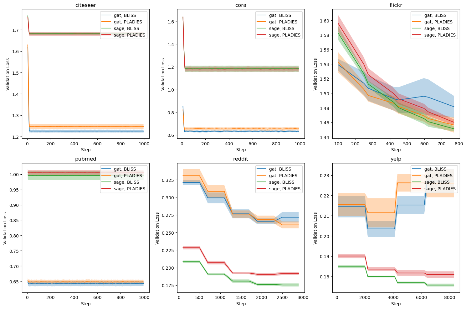
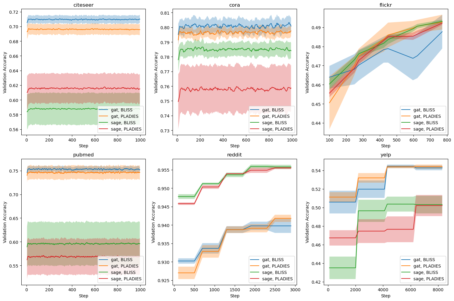
The remainder is organized as follows: section 2 describes BLISS; section 3 reports results; section 4 concludes. A detailed background and related work appear in sections B and C.
2 Proposed Method 2.1 Bandit-Based Layer Importance Sampling Strategy (BLISS) BLISS selects informative neighbors per node and layer via a policy-based approach, guided by a dynamically updated sampling distribution driven by rewards reflecting each neighbor’s contribution to node representation. Using bandit algorithms, BLISS balances exploration and exploitation, adapts to evolving embeddings, and maintains scalability on large graphs. Traditional node sampling often fails to manage this trade-off or adapt to changing node importance, reducing accuracy and scalability. While Liu et al. [2020] framed node-wise sampling as a bandit problem, BLISS extends it to layer-wise sampling, leveraging inter-layer information flow and reducing redundancy (see fig. 1).
Initially, edge weights w ij = 1 for all j ∈ N i , with sampling probabilities q ij set proportionally. BLISS proceeds top-down from the final layer L, computing layer-wise sampling probabilities p j for nodes in layer l. These are passed to algorithm 4, which selects k nodes. The GNN then performs a forward pass, where each node i aggregates from sampled neighbors j s to approximate its representation μi :
Here, j s ∼ q i denotes the s-th sampled neighbor of node i, drawn from the per-node sampling distribution q i . This process updates node representations h j . The informativeness of neighbors is quantified as a reward r ij , and the estimated rewards rij are calculated as:
where S t i is the set of sampled neighbors at step t, α ij is the aggregation coefficient, and h j is the node embedding. The edge weights w ij and sampling probabilities q ij are updated using the EXP3 algorithm (see algorithm 5). The edge weights are updated as follows:
where δ is a scaling factor and η is the bandit learning rate.
BLISS operates through an iterative process of four steps: (1) dynamically selecting nodes at each layer via a bandit algorithm (e.g., EXP3) that assigns sampling probabilities, (2) estimating node representations by aggregating from samp
This content is AI-processed based on open access ArXiv data.