Gutenberg-Richter-like relations in physical systems

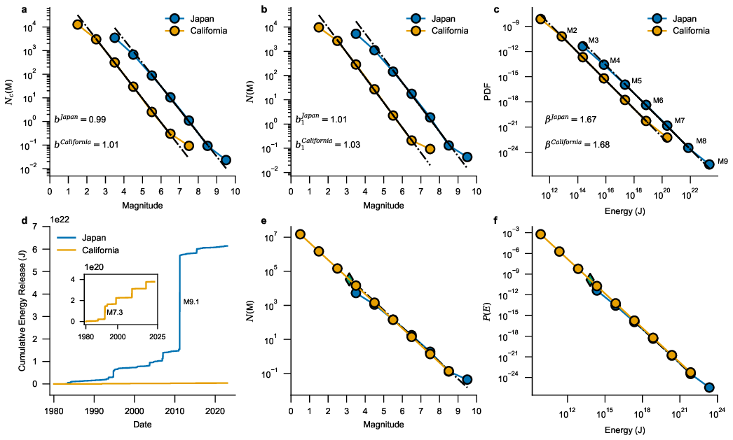
Gutenberg-Richter-like relations in physical systems K. Duplat,1 G. Varas,2 and O. Ramos1, ∗ 1Institut Lumi`ere Mati`ere, UMR5306 Universit´e Lyon 1-CNRS, Universit´e de Lyon 69622 Villeurbanne, France. 2Instituto de F´ısica, Pontificia Universidad Cat´olica de Valparaiso (PUCV), Avenida Universidad 330, Valparaiso, Chile. (Dated: December 22, 2025) We analyze regional earthquake energy statistics from the Southern California and Japan seismic catalogs and find scale-invariant energy distributions characterized by an exponent τ ≃1.67. 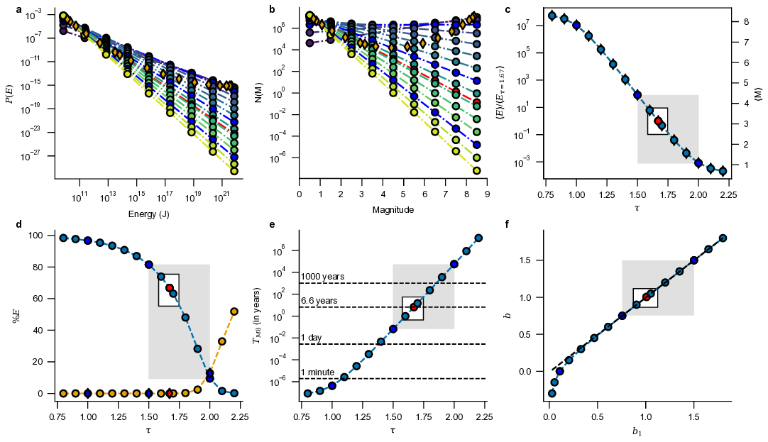To quantify how closely scale-invariant dynamics with different exponent values resemble real earthquakes, we generate synthetic energy distributions over a wide range of τ under conditions of constant activity. Earthquake-like behavior, in a broad sense, is obtained for 1.5 ⩽τ < 2.0. When energy variations are further restricted to be within a factor of ten relative to real earthquakes, the admissible range narrows to 1.58 ⩽τ ⩽1.76. We identify the physical mecha- nisms governing the dynamics in the different regimes: fault dynamics characterized by a balance between slow energy accumulation and release through scale-free events in the earthquake-like regime; externally supplied energy relative to a slowly driven fault for τ < 1.5; and dominance of small events in the energy budget for τ > 2. I. INTRODUCTION In many dissipative phenomena, including earthquakes [1], granular faults [2–7], sandpiles [8–10] and subcritical rup- ture [11–16], energy is slowly accumulated and then released through sudden events of all sizes, typically following power- law distributions. The scale-invariant nature of these events motivated theoreticians to draw on the formalism of phase transitions [17, 18]. Yet this raises a fundamental question: in natural systems, how is the fine-tuning of the order param- eter required to reach criticality achieved? [17] The idea of a critical point acting as an attractor of the dynamics, intro- duced by the Self-Organized Criticality (SOC) in 1987 [18], offered a compelling and elegant answer. Although SOC’s ambitious claims [19] and the absence of a unified theoretical framework attracted criticism [20, 21], the conceptual power of the idea galvanized leading figures in statistical physics [22, 23] and propelled its application to fields as diverse as seismology [24], neuroscience [25], and even financial markets [26]. Earthquakes were the most familiar, well-studied, and ar- guably the most relevant of these phenomena, and thus they quickly became the reference point for interpreting scale- invariant behavior. Regardless of the value of the power-law exponent τ in the event-size distribution P(s) ∼s−τ, the underlying interpretation remained the same: events occur across all scales, with numerous small ones and rare, catas- trophic ones that dominate the total energy release. In the 1990s, most laboratory experiments and earthquake catalogs lacked the precision needed to confront or guide the- oretical developments. Reported b-values in the Gutenberg- Richter (GR) law spanned a wide range [27], and no clear consensus existed on how to define an avalanche in a way that allowed meaningful comparison between theoretical or simu- lated τ exponents and those extracted from real data. From a theoretical standpoint, much of the effort focused on determining the value of τ and classifying avalanches into ∗osvanny.ramos@univ-lyon1.fr universality classes [28–32]. However, the extent to which the underlying dynamics differ across these classes was rarely examined, and they were often implicitly assumed to reflect the same earthquake-like behavior described above. With the ultimate goal of understanding the precise physi- cal scenario associated with a given exponent value, we begin by examining how avalanche sizes must be defined in order to compare them consistently. We then turn to the statistics of actual earthquakes, and finally analyze the different scenarios that arise when the exponent τ of the earthquake-size distri- bution is varied. II. AVALANCHE DEFINITION A central goal of this article is to clarify the physical scenar- ios associated with particular exponent values. As expected, however, different definitions of avalanche size lead to dis- tinct event distributions [33]. Consider a power law of the form P(s) = 1 N s−τ1, where N is a normalization constant. The variable s can be expressed as s = sDA l , where sl is the linear extent of the avalanche and DA its fractal dimension. Using this relation we obtain: P(s)ds = P(sl)dsl (1) 1 N s−τ1 DA l dA sDA−1 l dsl = P(sl)dsl (2) P(sl) = DA N s−τ2 l , where τ2 = (τ1 −1)DA + 1. (3) Thus, the same underlying process can be described by two power laws, P(s) and P(sl), characterized by different expo- nents, τ1 and τ2. Which definition should be considered the “correct” one? In the context of critical phenomena, event size is conventionally defined in terms of the event’s volume in an n-dimensional space [32, 34, 35]

This content is AI-processed based on open access ArXiv data.