3-manifolds are commonly represented as triangulations, consisting of abstract tetrahedra whose triangular faces are identified in pairs. The combinatorial sparsity of a triangulation, as measured by the treewidth of its dual graph, plays a fundamental role in the design of parameterized algorithms. In this work, we investigate algorithmic procedures that transform or modify a given triangulation while controlling specific sparsity parameters. First, we describe a linear-time algorithm that converts a given triangulation into a Heegaard diagram of the underlying 3-manifold, showing that the construction preserves treewidth. We apply this construction to exhibit a fixed-parameter tractable framework for computing Kuperberg's quantum invariants of 3-manifolds. Second, we present a quasi-linear-time algorithm that retriangulates a given triangulation into one with maximum edge valence of at most nine, while only moderately increasing the treewidth of the dual graph. Combining these two algorithms yields a quasi-linear-time algorithm that produces, from a given triangulation, a Heegaard diagram in which every attaching curve intersects at most nine others.
Structural properties of triangulations-which are commonly used to encode 3-manifolds both in theory and in practice-can dramatically affect the feasibility of computations. Over the past decade, several fixed-parameter tractable (FPT) algorithms have been developed that efficiently solve provably hard problems on 3-manifolds, provided they are represented by triangulations that are sufficiently "thin" [8,9,10,11,12]. 1 On input triangulations with bounded treewidth 2 these algorithms run in time polynomial in the number of tetrahedra. 3 Motivated by these algorithms, several recent papers have investigated the quantitative relationship between the treewidth (and other width parameters) of triangulations and the corresponding quantities in various related representations of 3-manifolds. It has been shown that 3-manifolds with small Heegaard genus [19,24], as well as hyperbolic 3-manifolds with small volume [23,35], admit triangulations with small treewidth. At the same time, for certain 3-manifolds, a large Heegaard genus or a "complicated" JSJ decomposition can entirely preclude the existence of triangulations with small treewidth [25,26]. 4 In this work, we also focus on algorithmic transformations of 3-manifold triangulations with a view toward parameterized algorithms and sparsity. We provide two main contributions.
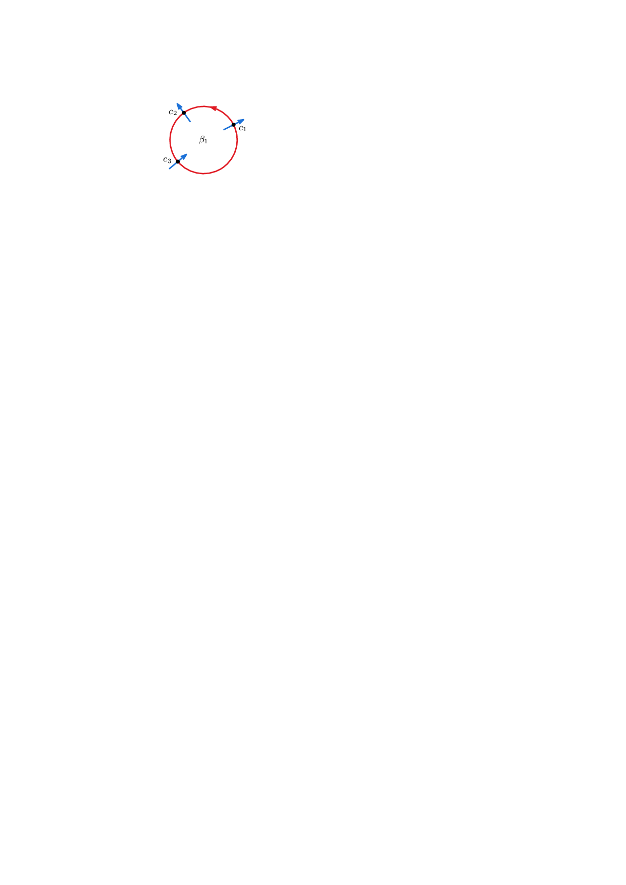
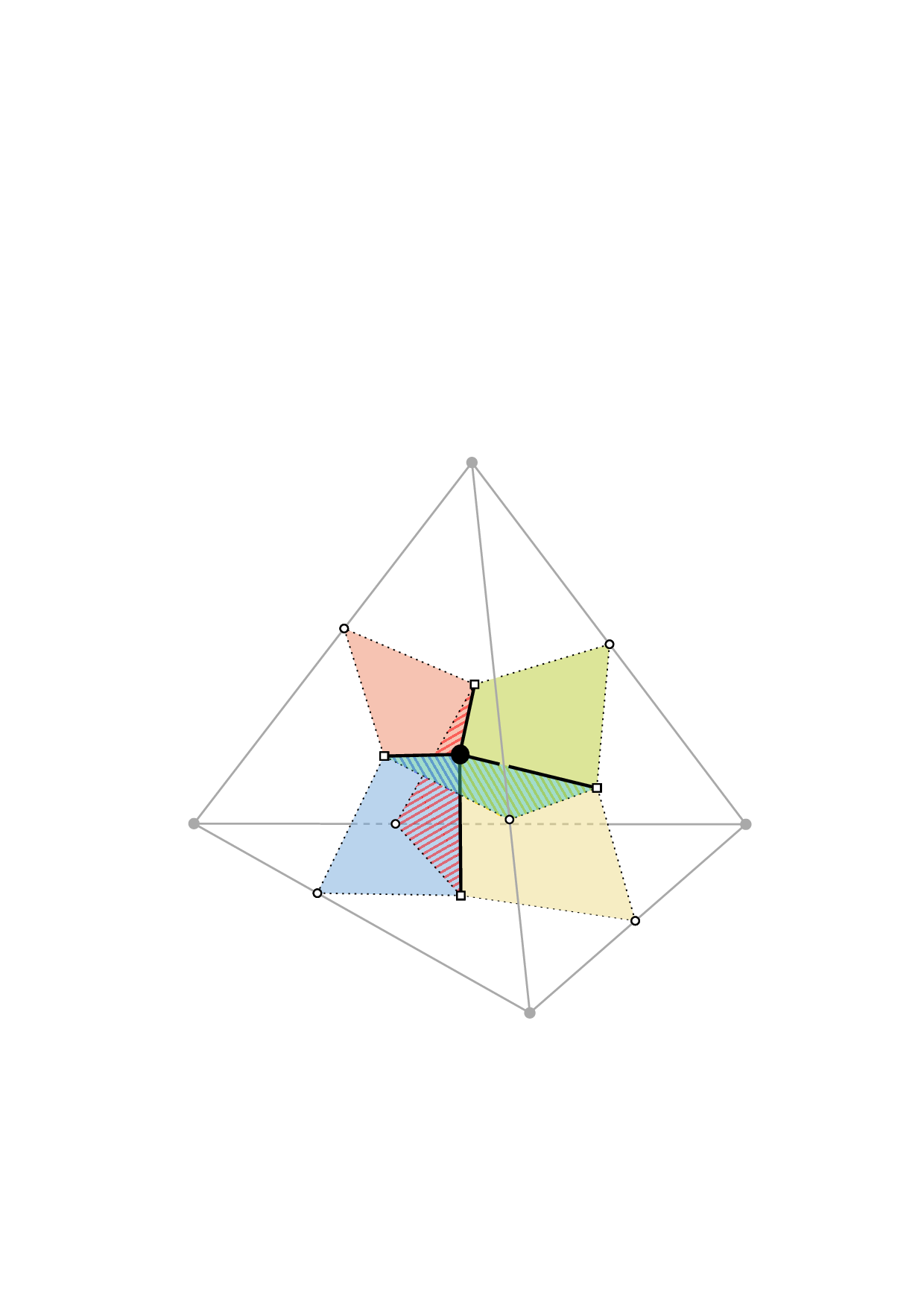
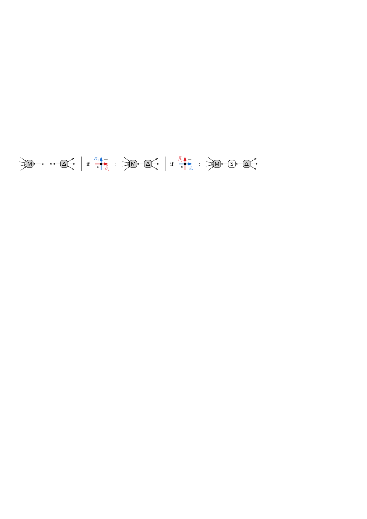
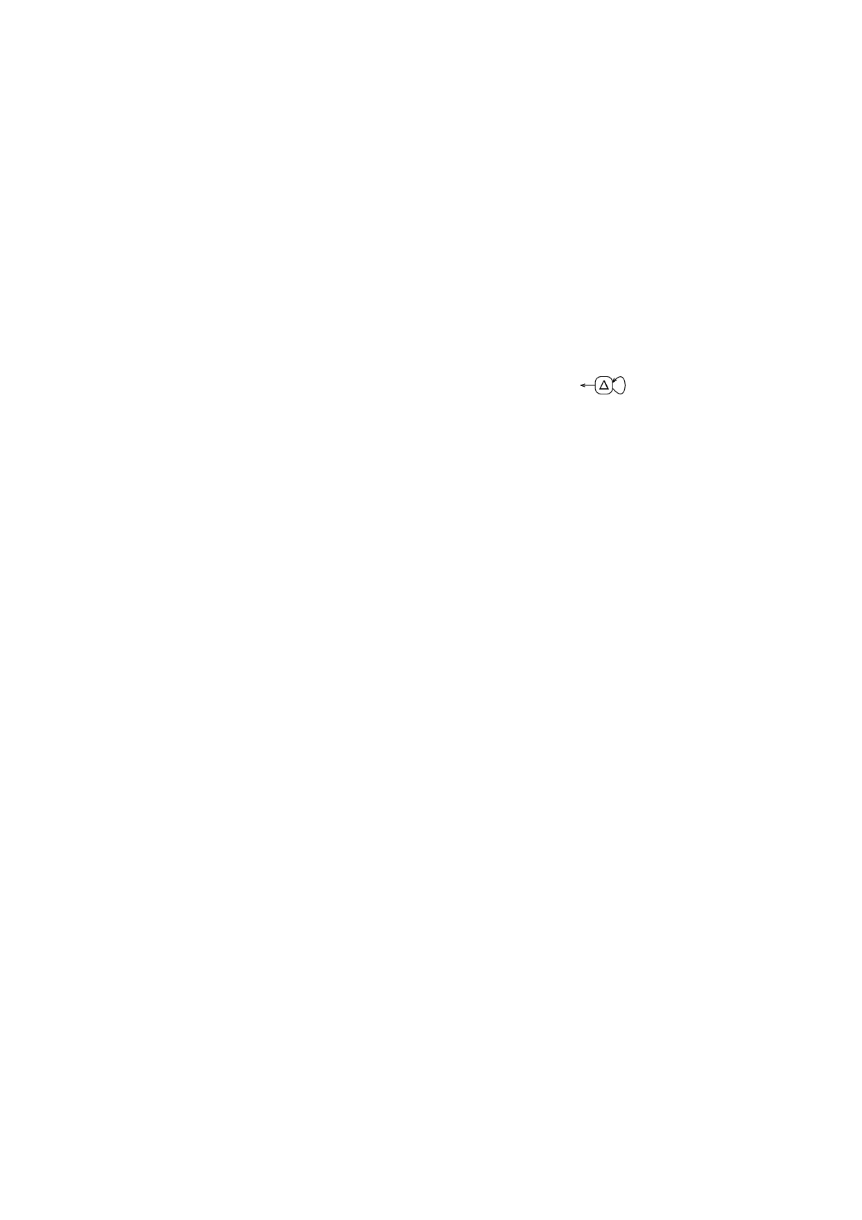
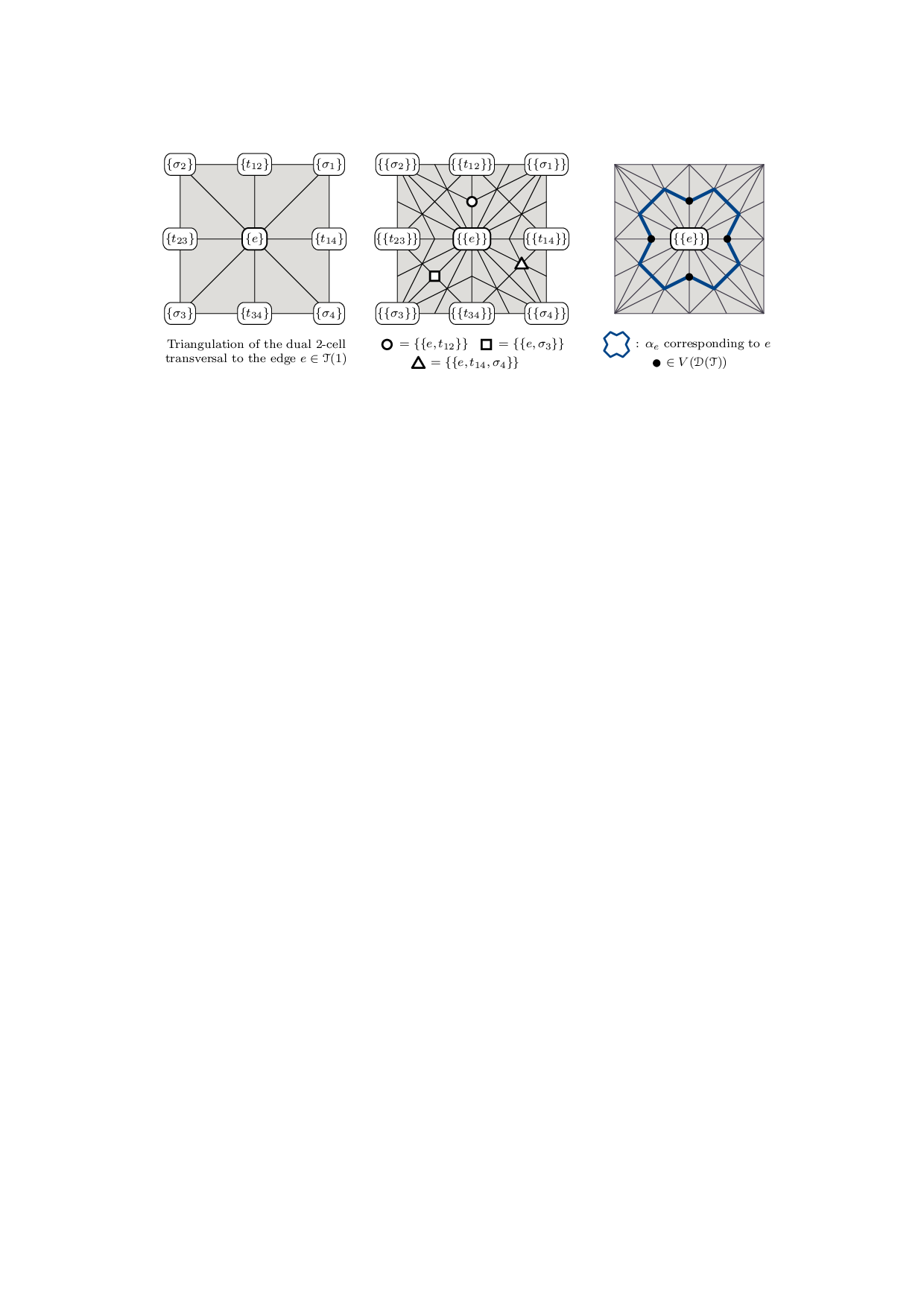
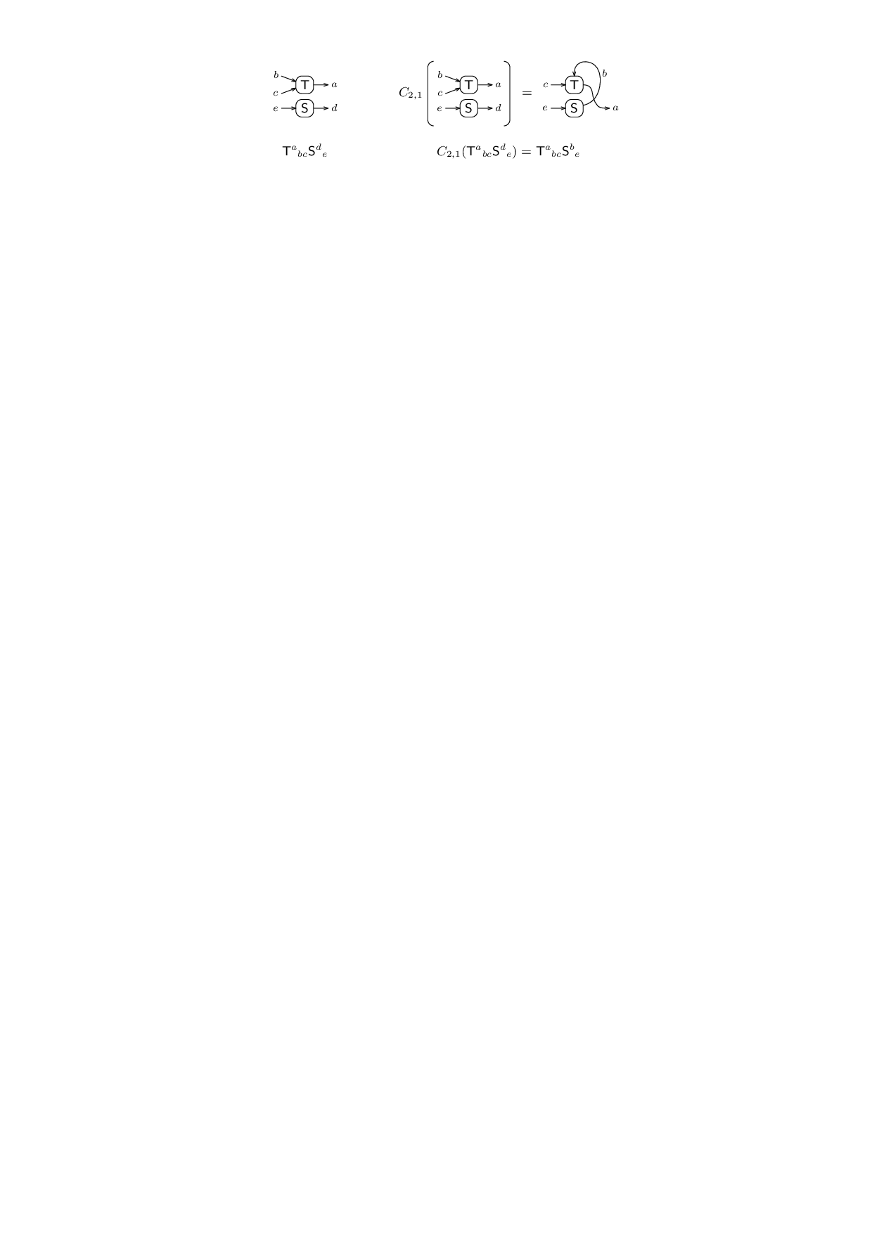
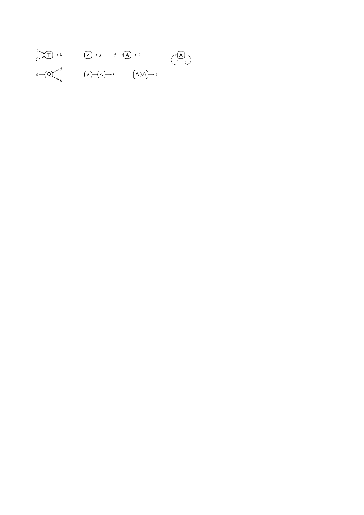
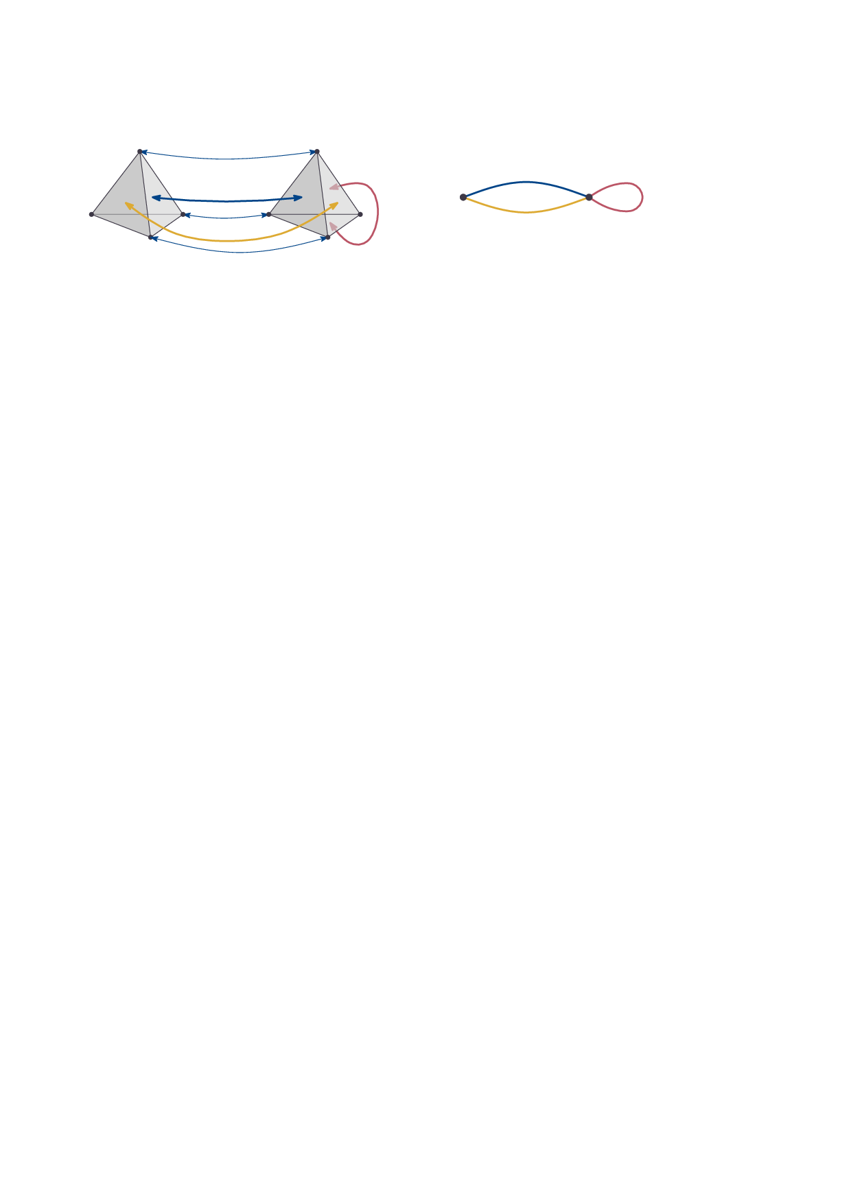
First, we revisit and analyze a classical construction that turns a triangulation T of a closed 3-manifold M into a Heegaard splitting and show that it yields a Heegaard diagram of M, whose size and treewidth are linearly bounded by those of T. More concretely, we prove ▶ Theorem 1. Let T be a triangulation of a closed, orientable 3-manifold M with n tetrahedra and dual graph Γ(T). Let D := D(T) be the Heegaard diagram of M induced by T. Then, for the number of vertices and for the treewidth 5 Guided by this result, in Section 5 we investigate the complexity of computing Kuperberg’s quantum invariants of oriented 3-manifolds [28], which are obtained from a Heegaard diagram by evaluating an associated tensor network. First, we show that this construction is widthpreserving (Lemma 18). This insight, combined with Theorem 1 and results on the complexity of evaluating tensor networks [37,40] (cf. Theorem 19), provides a framework for computing Kuperberg’s invariants from triangulations that is FPT in the treewidth (Theorem 15). ▶ Remark. The converse of Theorem 1, i.e., building a triangulation from a given Heegaard splitting in a width-preserving way, has been studied in [24] and, very recently, in [19], where an explicit algorithm for constructing a triangulation from a Heegaard diagram is provided.
Our second contribution investigates the interplay between the maximum edge valence and the treewidth of a 3-manifold triangulation T. Analogous to the notion of vertex degree in graphs, the valence of an edge in T is defined as the number of tetrahedra in T that contain it. While treewidth can be viewed as a measure of global sparsity, the maximum edge valence captures local sparsity. The maximum edge valence of a triangulation can also provide valuable insights into geometric properties of the underlying 3-manifold [16,Sec. 3.6]. Having a triangulation T with small maximum edge valence can be computationally advantageous even when T already has small treewidth; see Appendix A for a discussion.
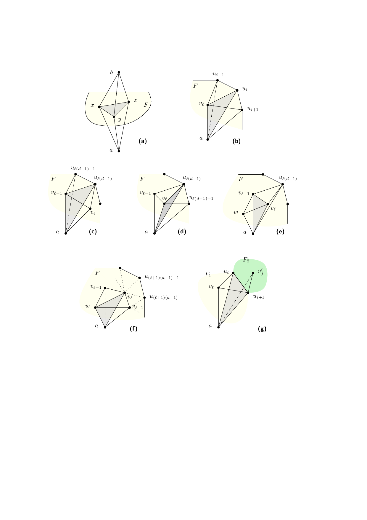
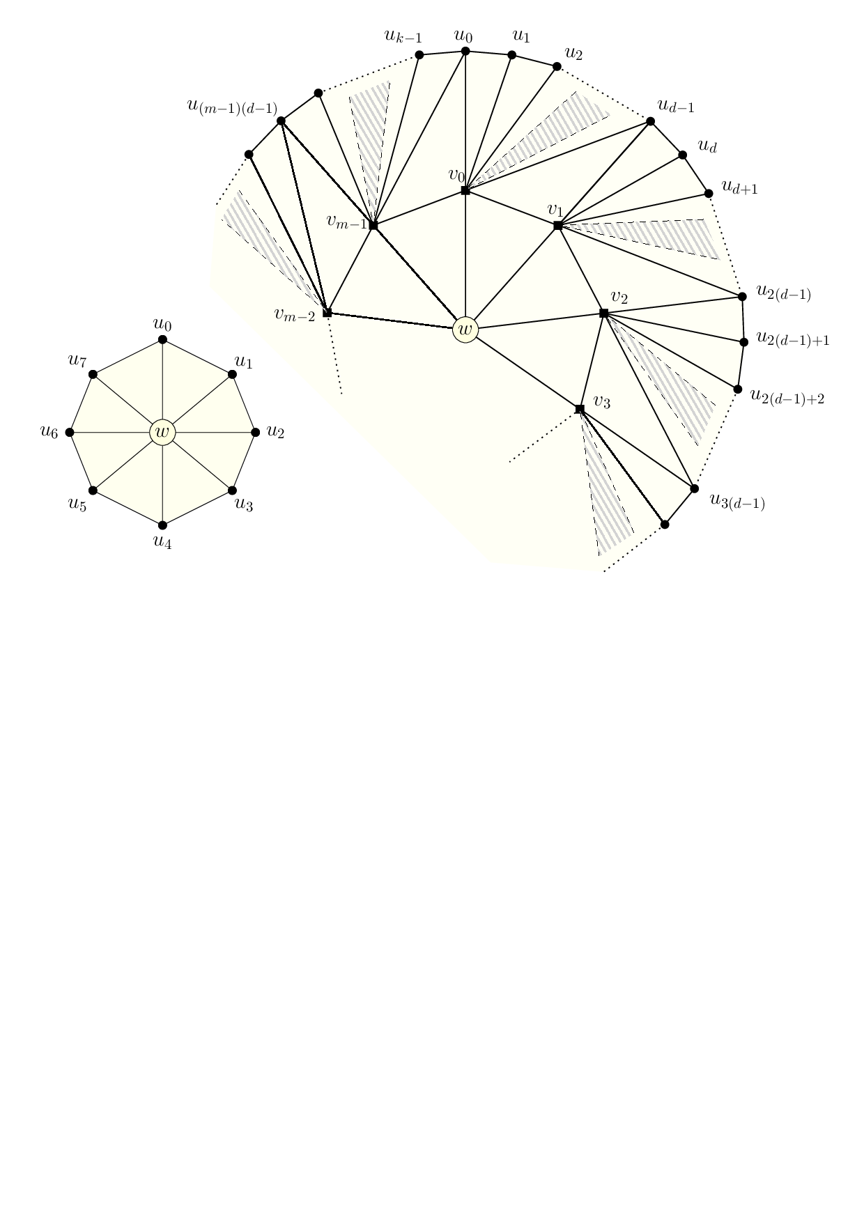
Every closed orientable 3-manifold has a triangulation with maximum edge valence at most six [4]. Frick has shown by an explicit construction that any triangulation T can be modified into a triangulation T † of the same manifold with edge valences at most nine [16,Theorem 3.36]. However, this construction may significantly increase the treewidth of the resulting triangulation, because if T contains edges with large valence, the retriangulation procedure introduces large grid-like structures in T † . In Section 4, we show how to circumvent this and obtain a different retriangulation T * that also achieves ∆(T * ) ≤ 9, while controlling the increase in treewidth by a polylogarithmic factor of the maximum edge valence of T.
▶ Theorem 2. There is an algorithm which, given a triangulation T of a closed 3-manifold M with n tetrahedra, v vertices, tw(Γ(T)) = tw, and maximum edge valence ∆(T) = ∆, constructs a triangulation T * of M with O((n + v) • poly(log 2 (∆))) vertices and tetrahedra, tw(Γ(T * )) ≤ tw • poly(log 2 (∆)), and ∆(T * ) ≤ 9. The algorithm runs in O(n log log n) time.
Finally, the execution of the algorithms in Theorem 2 and Theorem 1 (in this order) yields the following corollary, which we believe to be of independent interest.
By a graph we generally mean a multigraph G = (V, E) with a finite set V = V (G) of vertices and of a multiset E = E(G) of two-element submultisets of V called edges. A loop is an edge of the form {v, v}, and a multiedge is an edge with multiplicity larger than one. A graph without loops or multiedges is simple.
Introduced in [42] (cf. [15]), the treewidth of a gr
This content is AI-processed based on open access ArXiv data.