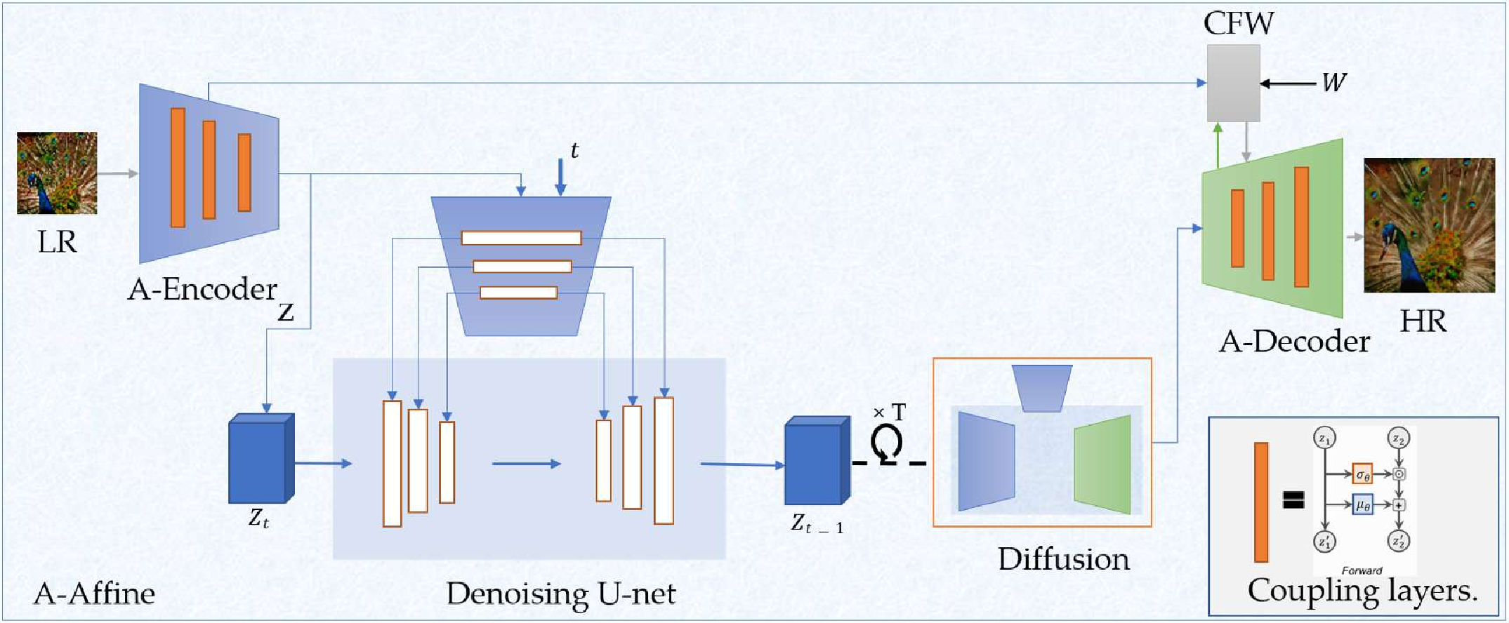
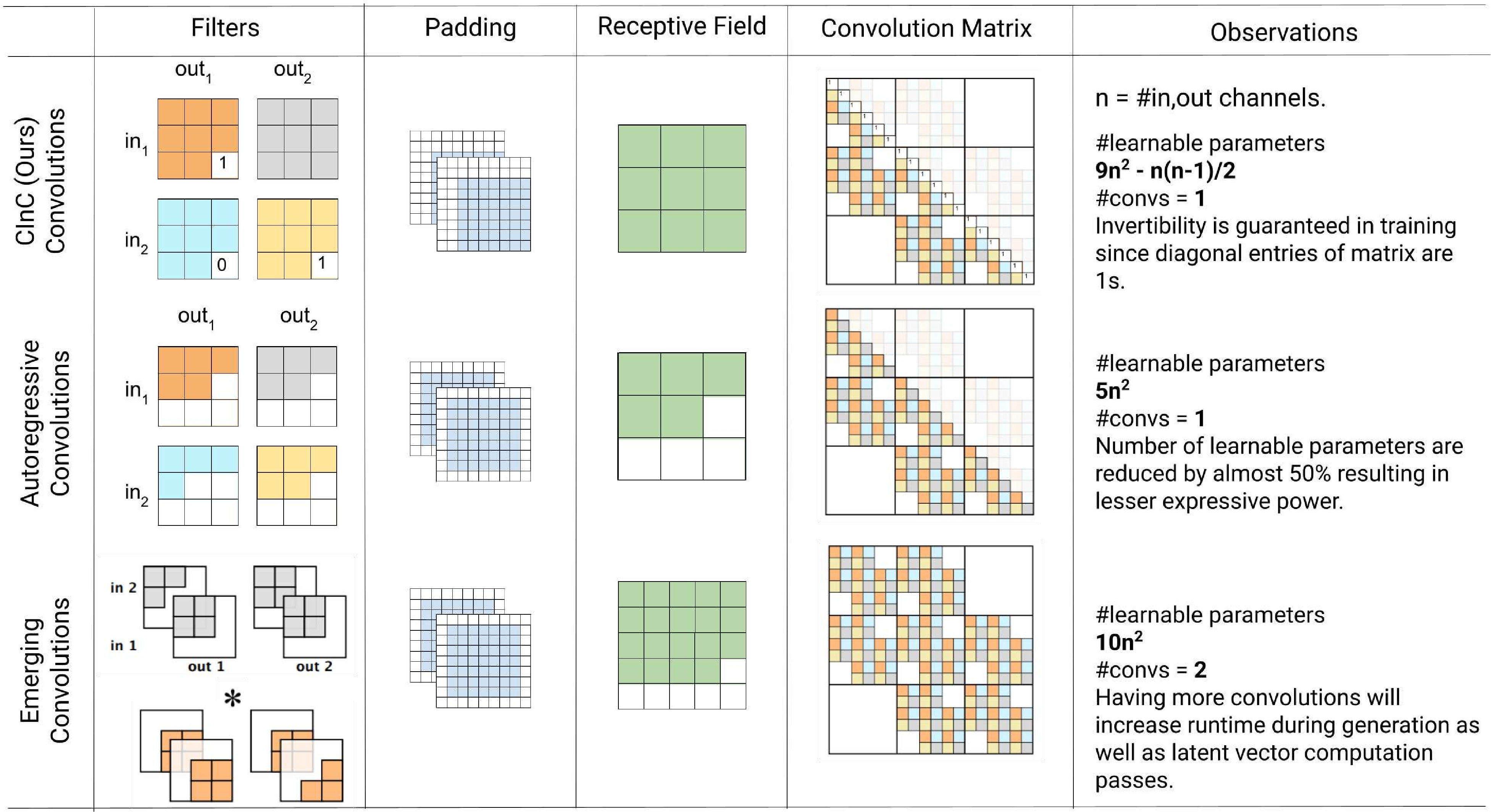
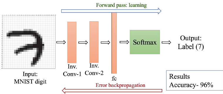
This thesis presents novel contributions in two primary areas: advancing the efficiency of generative models, particularly normalizing flows, and applying generative models to solve real-world computer vision challenges. The first part introduce significant improvements to normalizing flow architectures through six key innovations: 1) Development of invertible 3x3 Convolution layers with mathematically proven necessary and sufficient conditions for invertibility, (2) introduction of a more efficient Quad-coupling layer, 3) Design of a fast and efficient parallel inversion algorithm for kxk convolutional layers, 4) Fast & efficient backpropagation algorithm for inverse of convolution, 5) Using inverse of convolution, in Inverse-Flow, for the forward pass and training it using proposed backpropagation algorithm, and 6) Affine-StableSR, a compact and efficient super-resolution model that leverages pre-trained weights and Normalizing Flow layers to reduce parameter count while maintaining performance.
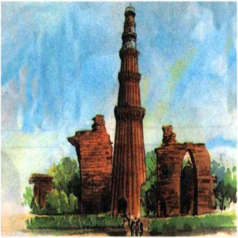
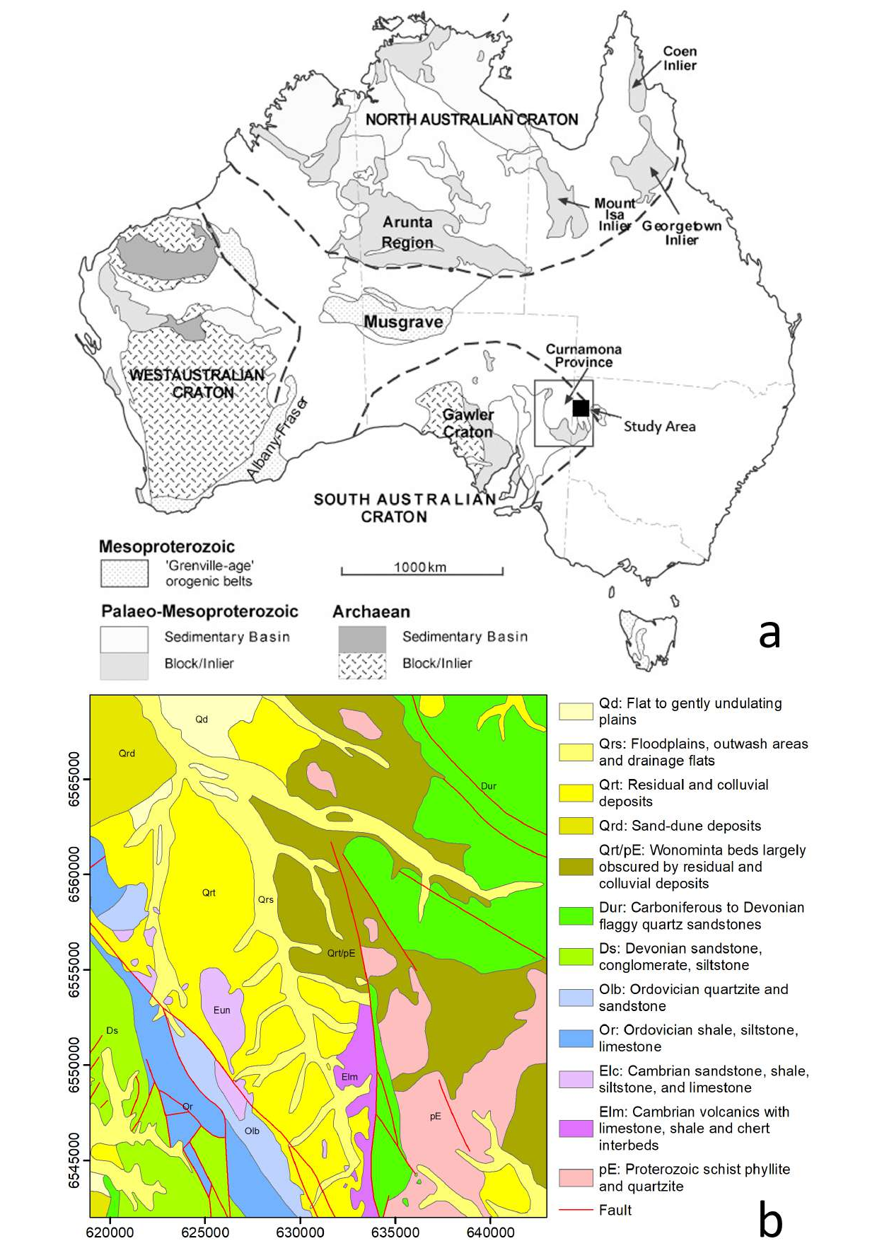
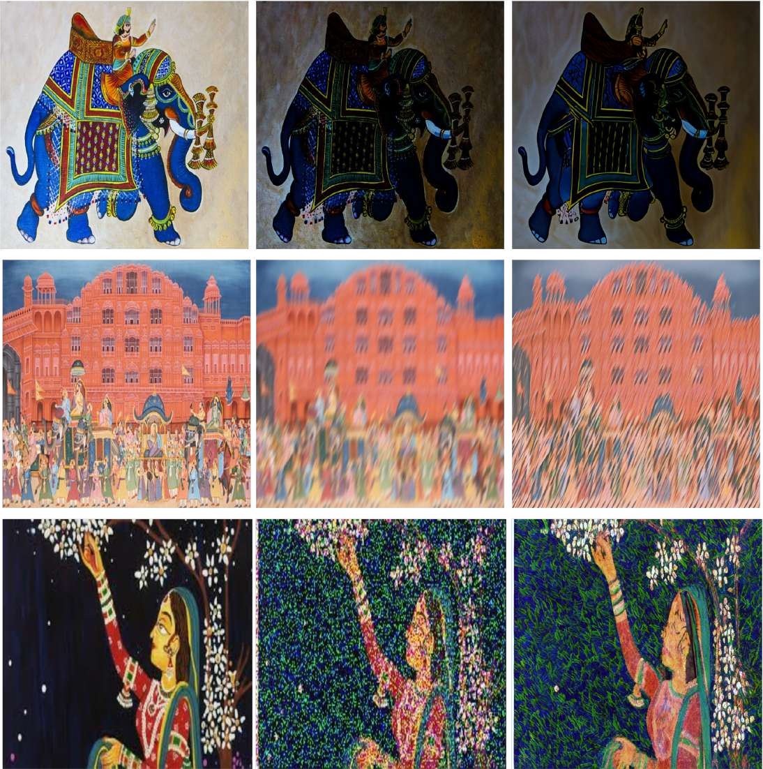
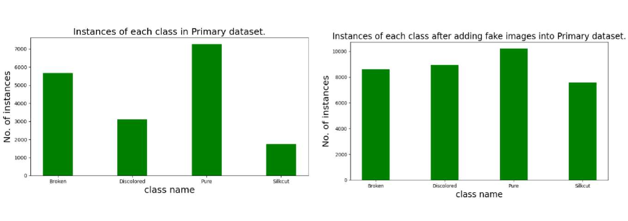
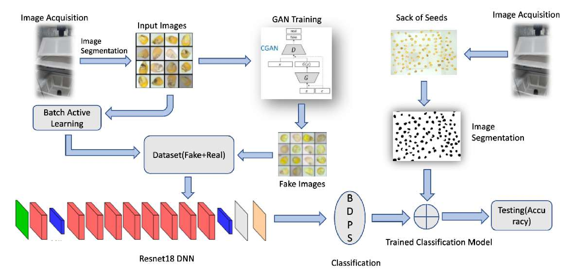
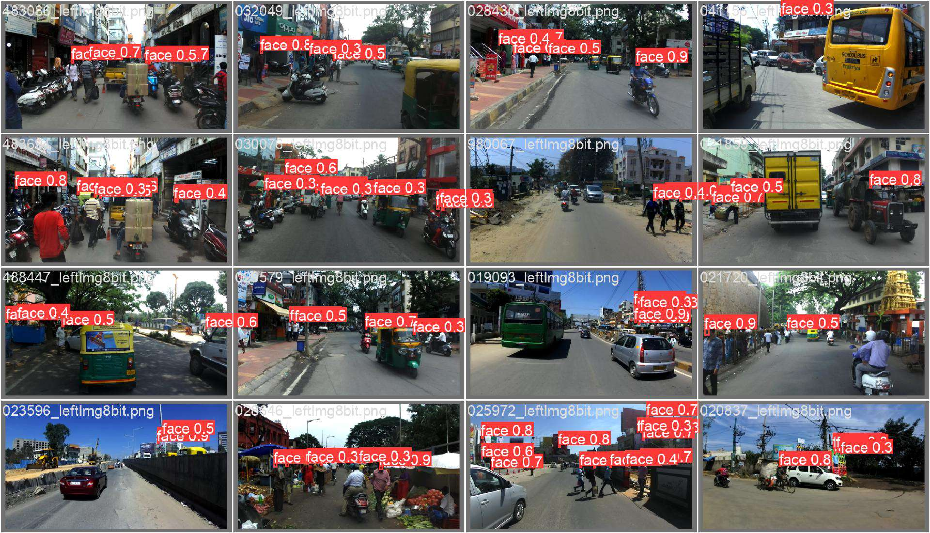
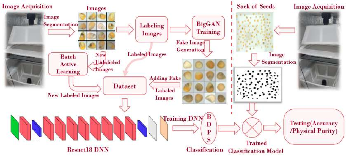
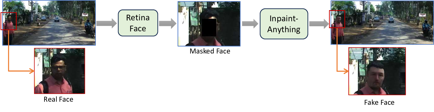
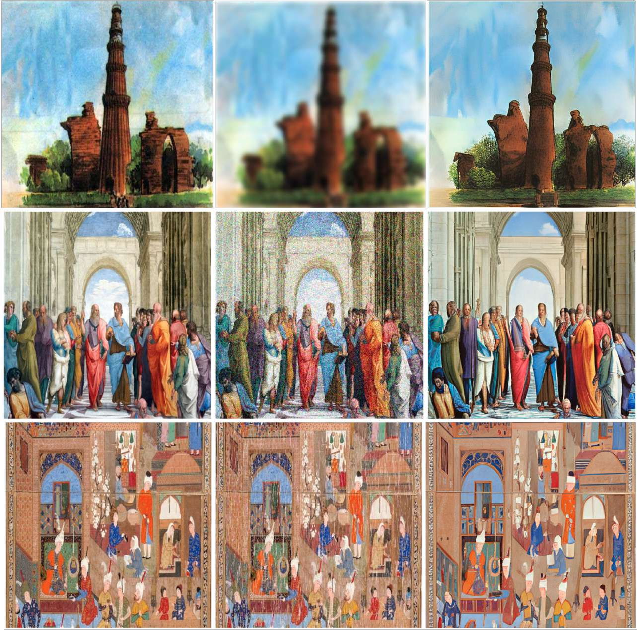
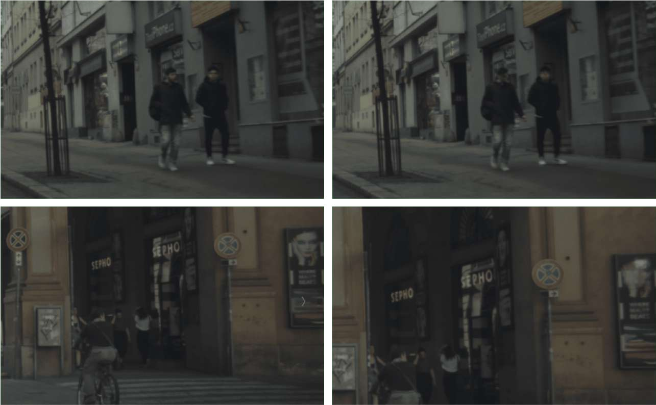
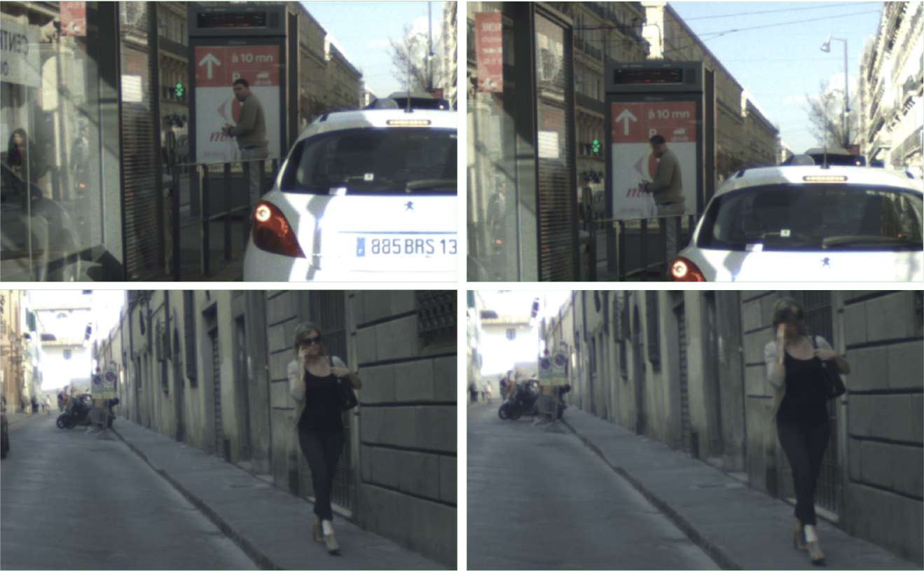
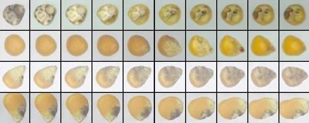
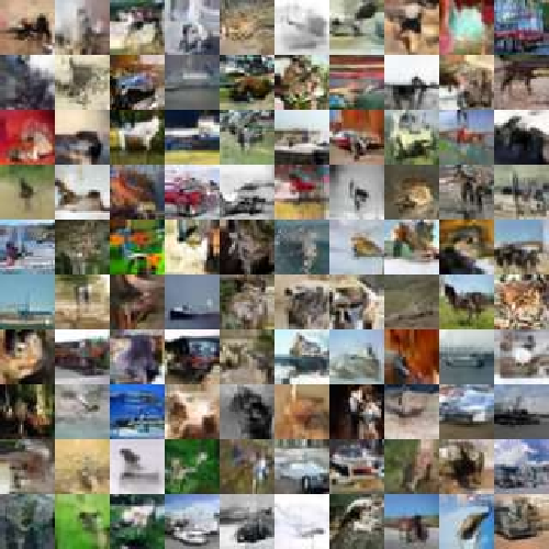
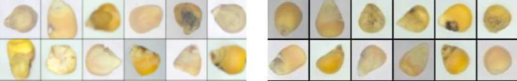
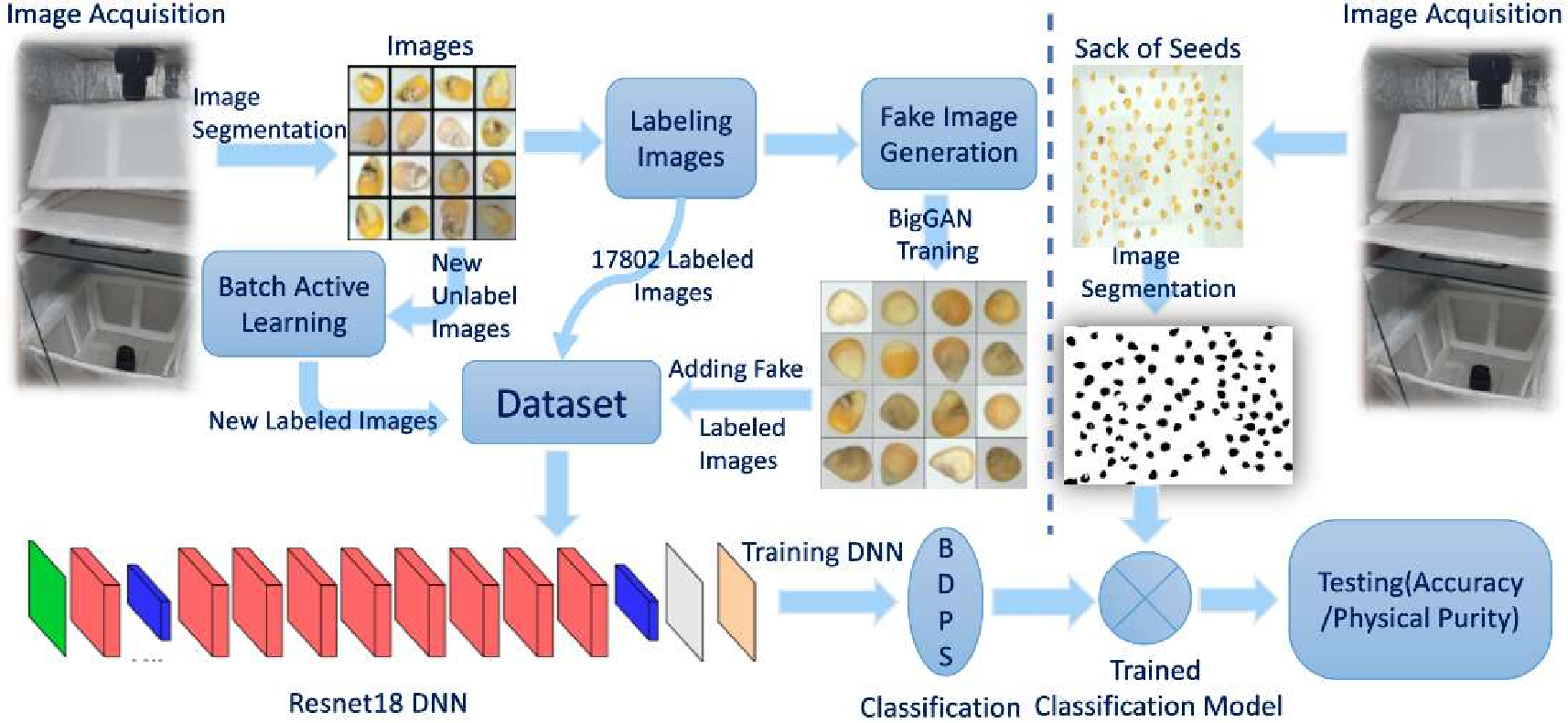
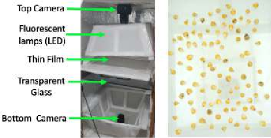
The second part: 1) An automated quality assessment system for agricultural produce using Conditional GANs to address class imbalance, data scarcity and annotation challenges, achieving good accuracy in seed purity testing; 2) An unsupervised geological mapping framework utilizing stacked autoencoders for dimensionality reduction, showing improved feature extraction compared to conventional methods; 3) We proposed a privacy preserving method for autonomous driving datasets using on face detection and image inpainting; 4) Utilizing Stable Diffusion based image inpainting for replacing the detected face and license plate to advancing privacy-preserving techniques and ethical considerations in the field.; and 5) An adapted diffusion model for art restoration that effectively handles multiple types of degradation through unified fine-tuning.
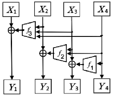
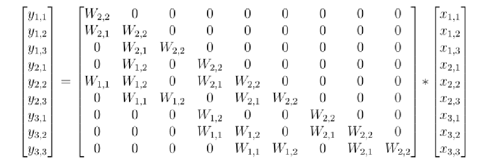
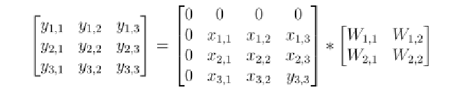
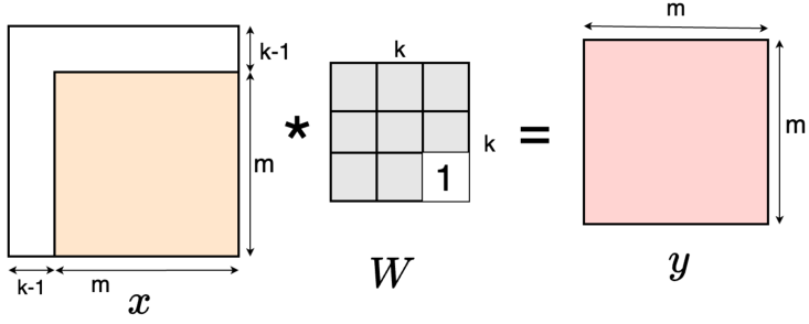
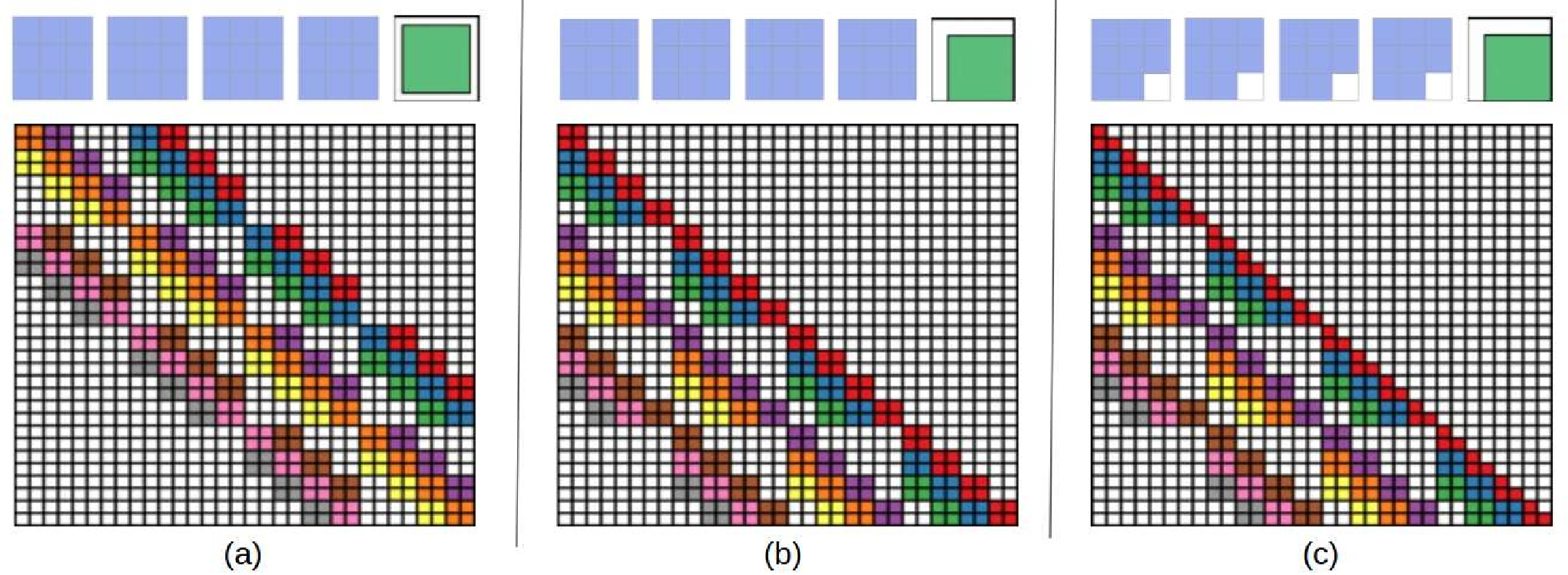
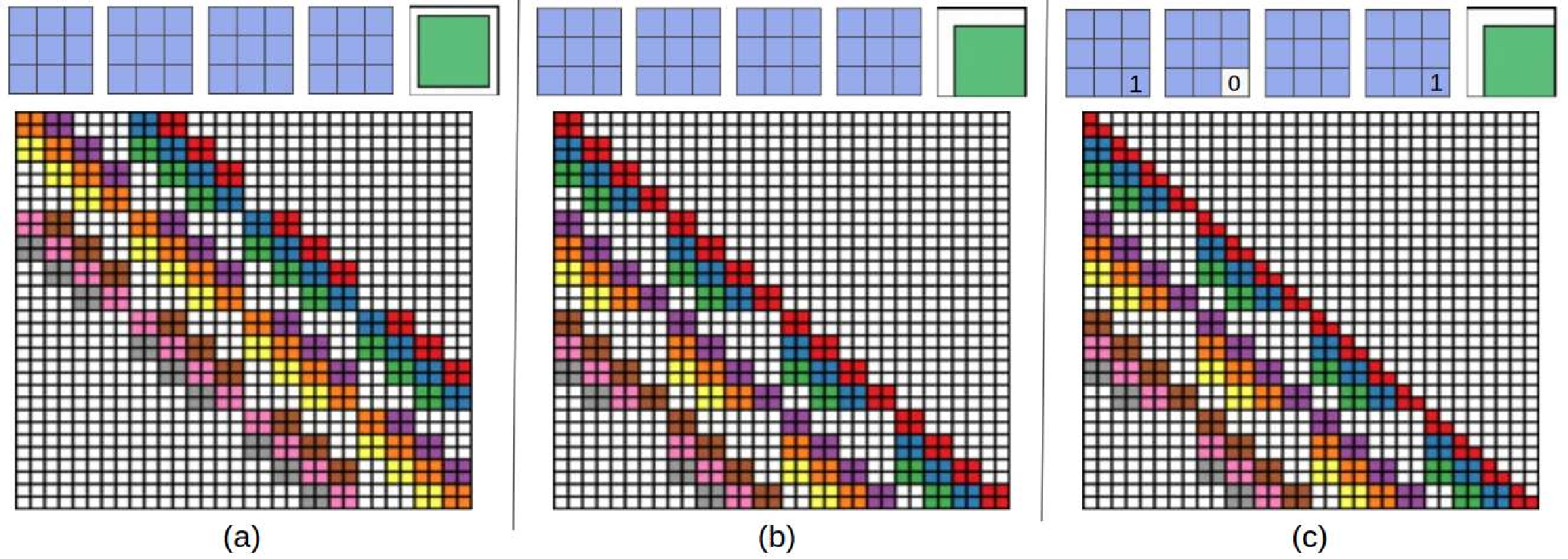
.Top: The first four are the kernel matrix, and the fifth is the input matrix with the standard padding that gives the bottom convolution matrix. Bottom: the convolution matrix corresponding to a convolution with a kernel of size three applied to an input of size 4 × 4, padded on both sides, and with two channels. Zero coefficients are drawn in white; other coefficients are drawn using the same color if applied to the same spatial location, albeit on different channels. (b) Top: an alternative padding scheme that results in a block triangular matrix M , Bottom: The matrix corresponding to a convolution with a kernel of size three applied to an input of size 4 × 4 padded only on one side and with two channels. (c) Top: an masked alternative padding scheme that results in a triangular matrix M , Bottom: the matrix corresponding to a convolution with a kernel of size three applied to an input of size 4 × 4 padded only on one side and with two channels. One of the weights of the kernel is masked. Note that the equivalent matrix M is triangular. . . . . . . . . . . . . . . . . . . . . . . . . . . . . . . . . . [11] comparison of the speed and utilization of parameters with Autoregressive convolutions and Emerging convolutions. . . . . . x 2. 4 The Quad-coupling layer, each input block X i has the same spatial dimension as the input X but only one-quarter of the channels. Each function f 1 , f 2 , and f 3 is a 3-layer convolutional network.
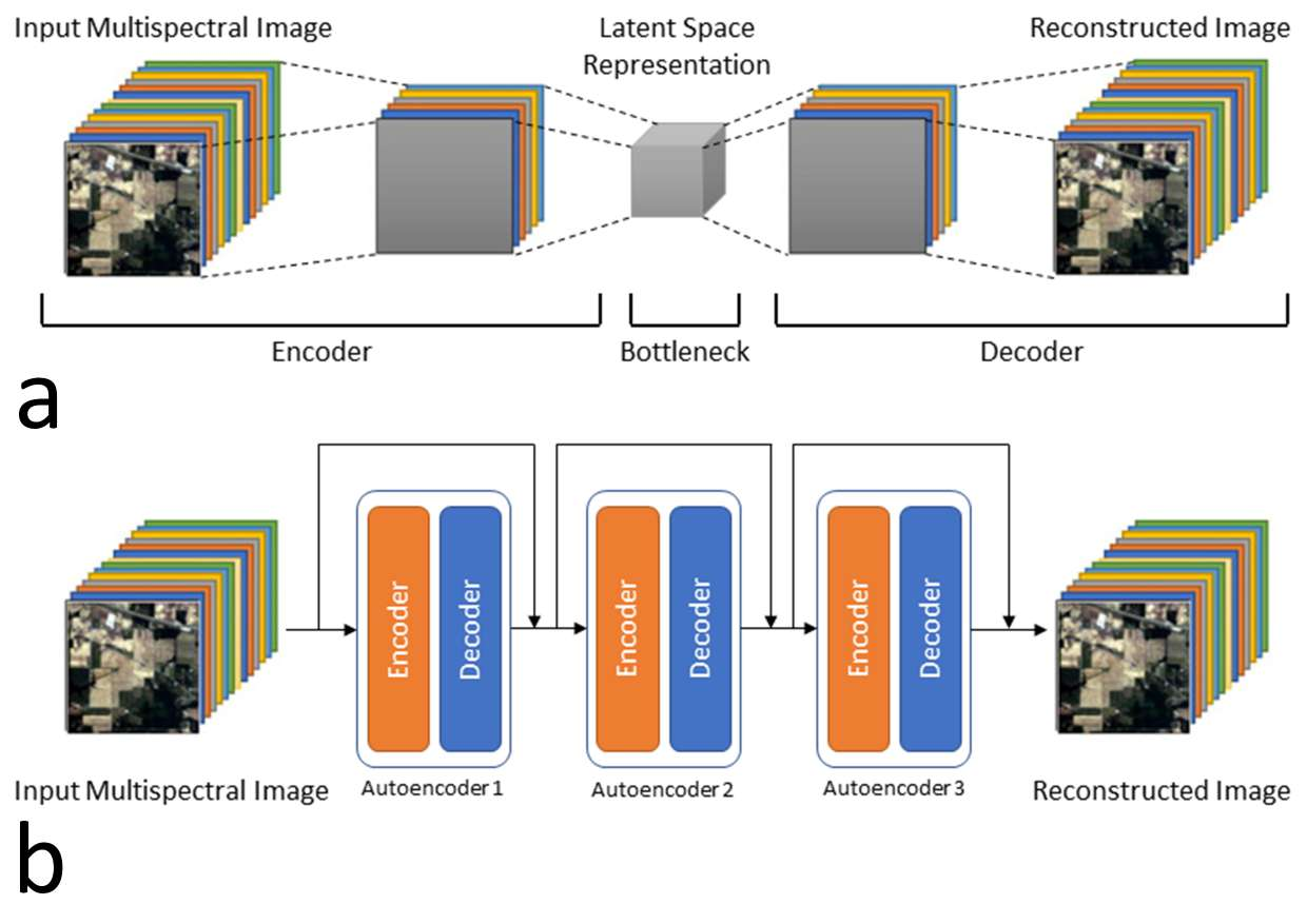
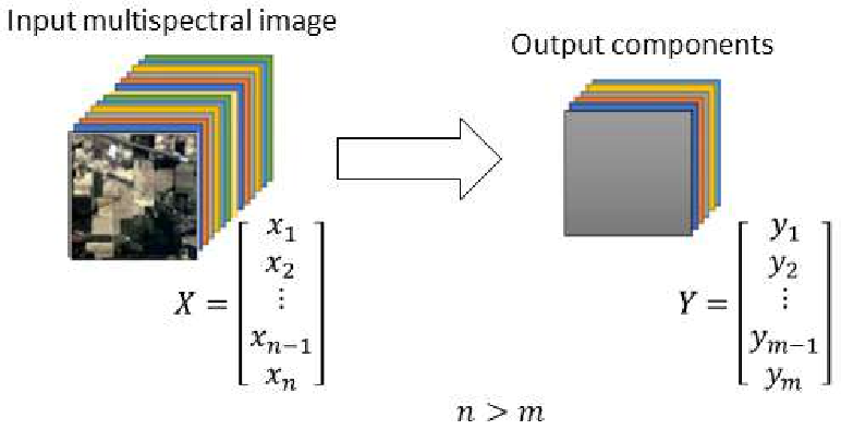
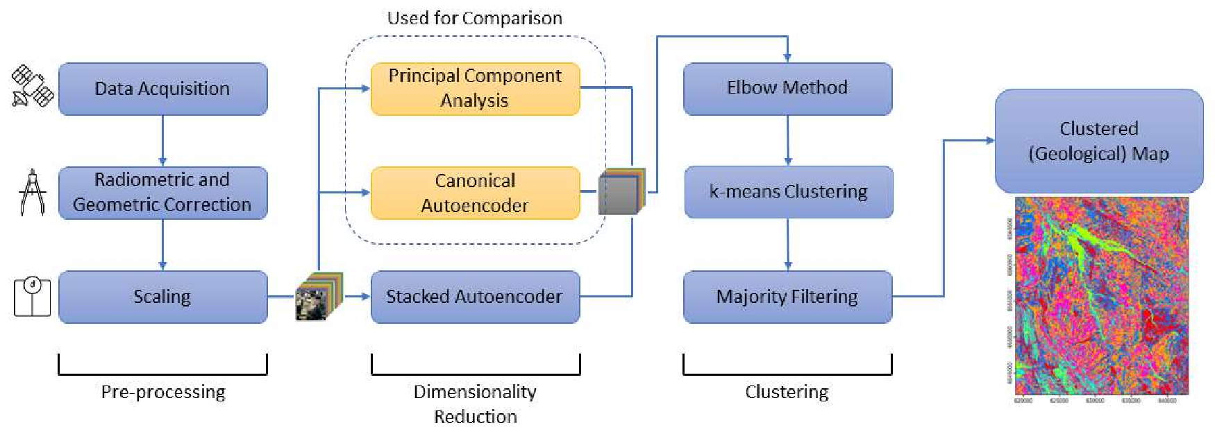
The architecture of a canonical autoencoder consists of an encoder and a decoder. The encoder takes the multispectral image as input (x) and reduces the dimension to the latent vector (z), where dim(x) >= dim(z). The decoder reconstructs the image from the latent vector (Z). b) A stacked autoencoder with three encoders and decoders for each stacking level. Each stack level’s encoder and decoder architecture is the same as the canonical autoencoder, with a number of hidden layers for each. . . . . . . . . . . . . . . . . . . . . . . . . . . . . . . . . . . 7.4 The visualization of the dimensionality reduction for a multispectral dataset. The number of input spectral bands n is reduced to m in the output dataset. Each colored layer in the input image and the output represents a spectral band and a component, respectively. . . . . . . . 7.5 Machine learning framework for creating geological maps using the integration of the dimensionality reduction (PCA, canonical autoencoder, and stacked autoencoder) methods and the k-means clustering.
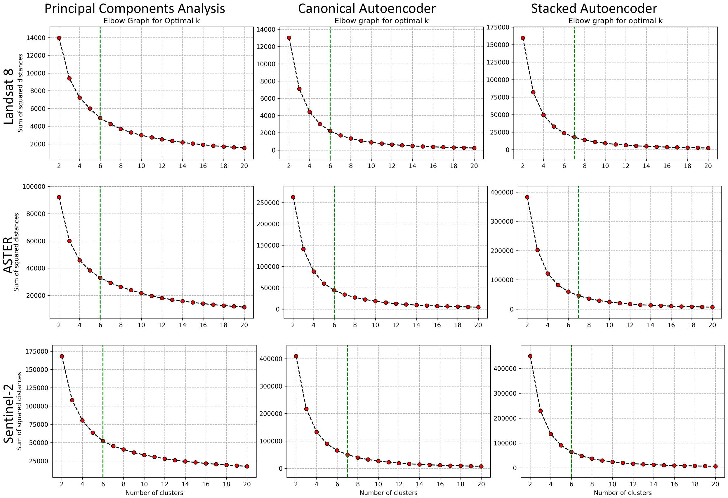
7.6 Elbow plots used to determine the optimal number of clusters (k) for each combination of remote sensing data (Landsat 8, ASTER, Sentinel-2) and dimensionality reduction method (PCA, canonical autoencoder, stacked autoencoder). The x-axis shows the number of clusters, and the y-axis represents the sum of squared distances to the cluster centers.
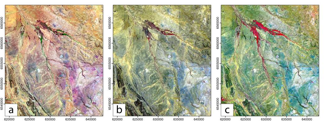
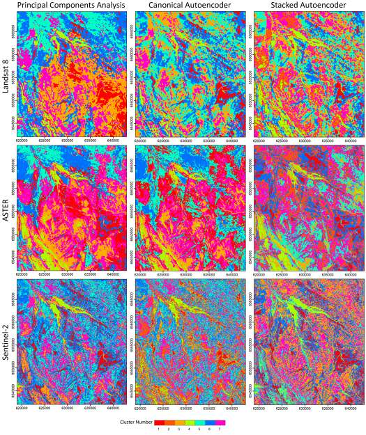
The point of maximum curvature in each plot, identified by the green dashed line, indicates the optimal value of k. . . . . . . . . . . . . . . xiii 7.7 Clustered maps of the study area obtained by different pairs of data types and dimensionality reduction methods. Each distinct colored region in the maps represents a unique geological unit on the ground.
We find that PCA (first column) generally results in less detailed geological unit differentiation than autoencoder-based methods, reflecting its limitations in capturing complex nonlinear relationships in the data. Sentinel-2 data (last row) shows the best cluster compactness ResShift. The restored outputs demonstrate substantial visual improvement and detail recovery compared to the degraded inputs, indicating the effectiveness of the proposed approach. . . . . . . . . . . . 9.1 Examples of frame-level traffic sign annotations in the MTSVD [227].
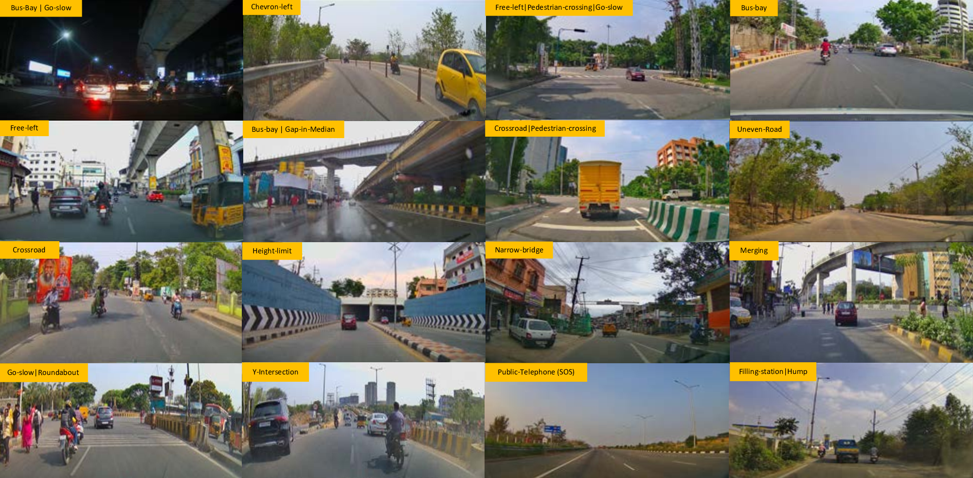
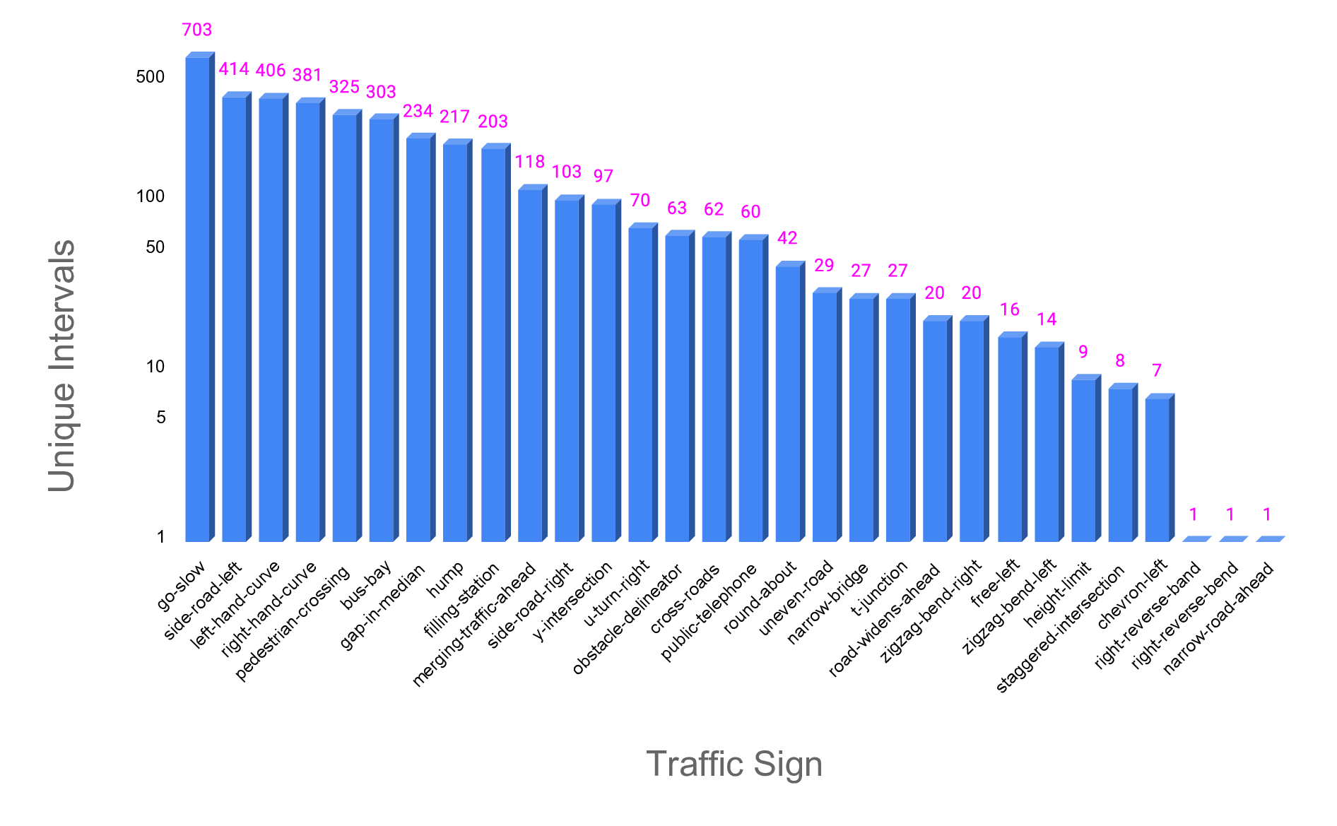
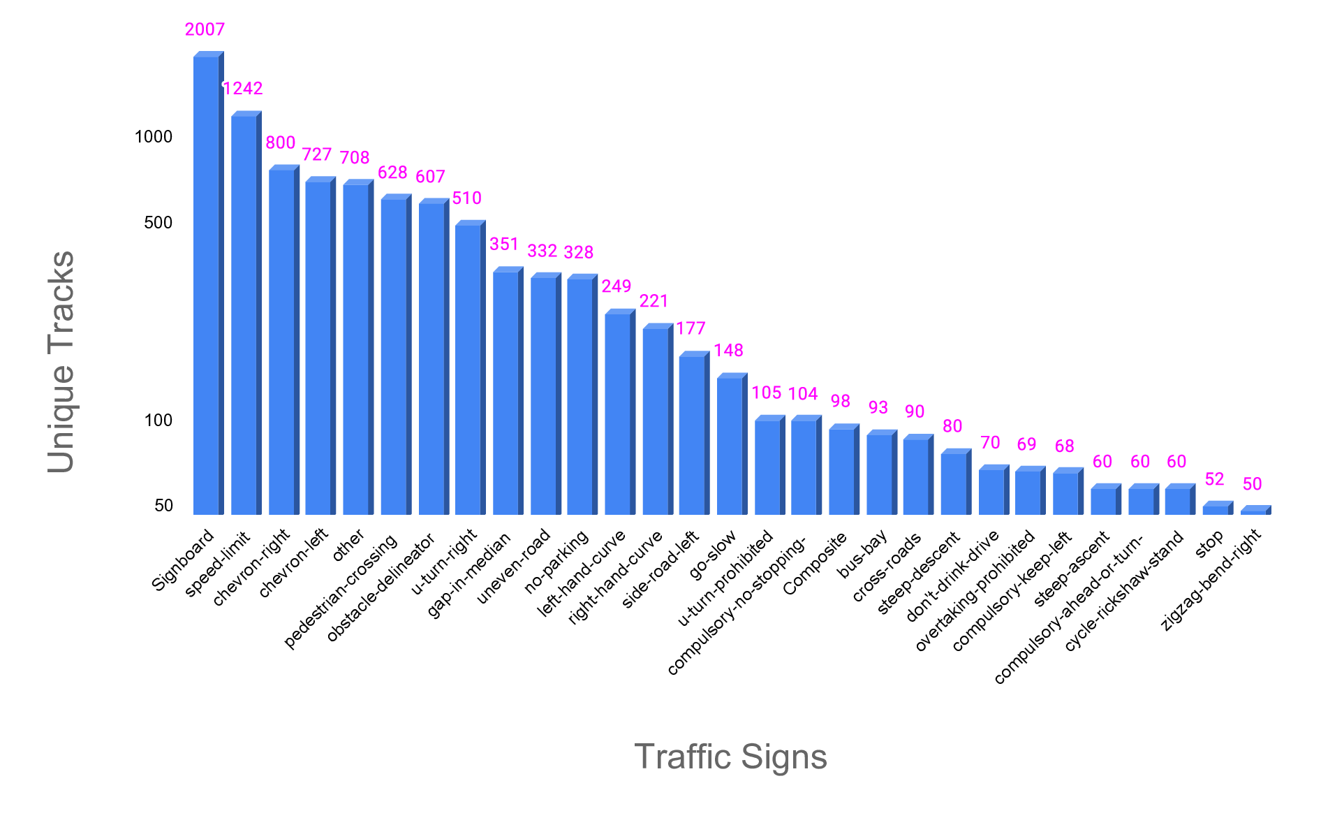
Each frame includes bounding-box tracks for traffic signs, annotated with type, track ID, and visual attributes such as tilted, occluded, and non-standard. The dataset captures a variety of sign types across diverse lighting and weather conditions, contributing to its robustness for real-world scene understanding and detection tasks. . . . . . . . . 9.2 Illustrative examples of contextual scene categories from the MTSVD, where the associated traffic sign is missing. These scenes demonstrate a variety of real-world road environments such as pedestrian crossings, bus bays, sharp curves, and merging roads, each containing consistent contextual cues despite the absence of the expected traffic sign. Such context-driven patterns are critical for learning-based models to infer missing traffic signage and enable effective scene categorization [227]. xv 9.3 Distribution of the top 30 most frequent traffic signs in the MTSVD dataset, represented by the number of unique annotated tracks. Statistics of traffic sign annotations in the Missing Traffic Signs Video Dataset (MTSVD). These statistics highlight the imbalance in traffic sign presence and absence within the dataset, reflecting real-world scenarios where cer
This content is AI-processed based on open access ArXiv data.