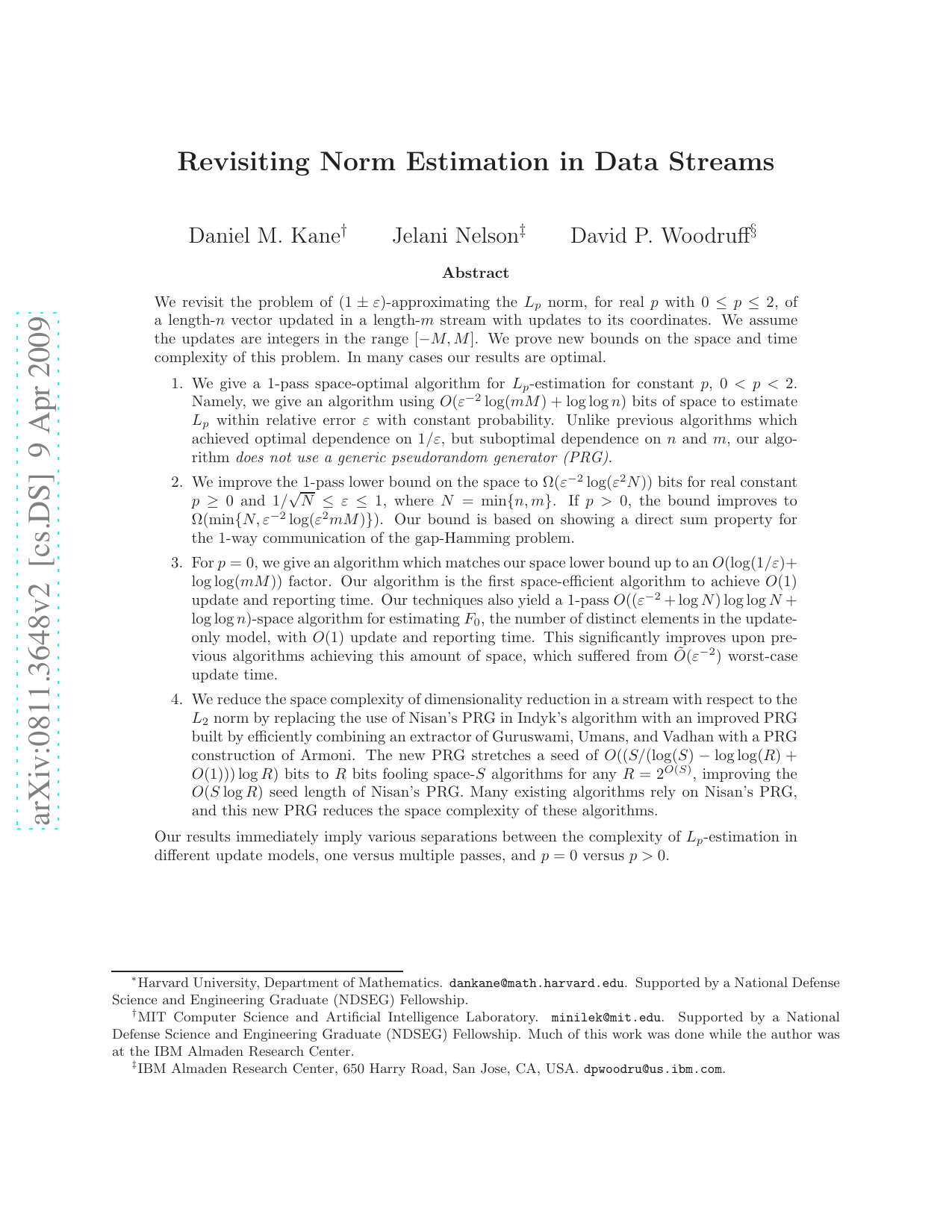
The problem of estimating the pth moment F_p (p nonnegative and real) in data streams is as follows. There is a vector x which starts at 0, and many updates of the form x_i <-- x_i + v come sequentially in a stream. The algorithm also receives an error parameter 0 < eps < 1. The goal is then to output an approximation with relative error at most eps to F_p = ||x||_p^p. Previously, it was known that polylogarithmic space (in the vector length n) was achievable if and only if p <= 2. We make several new contributions in this regime, including: (*) An optimal space algorithm for 0 < p < 2, which, unlike previous algorithms which had optimal dependence on 1/eps but sub-optimal dependence on n, does not rely on a generic pseudorandom generator. (*) A near-optimal space algorithm for p = 0 with optimal update and query time. (*) A near-optimal space algorithm for the "distinct elements" problem (p = 0 and all updates have v = 1) with optimal update and query time. (*) Improved L_2 --> L_2 dimensionality reduction in a stream. (*) New 1-pass lower bounds to show optimality and near-optimality of our algorithms, as well as of some previous algorithms (the "AMS sketch" for p = 2, and the L_1-difference algorithm of Feigenbaum et al.). As corollaries of our work, we also obtain a few separations in the complexity of moment estimation problems: F_0 in 1 pass vs. 2 passes, p = 0 vs. p > 0, and F_0 with strictly positive updates vs. arbitrary updates.
Computing over massive data streams is increasingly important. Large data sets, such as sensor networks, transaction data, the web, and network traffic, have grown at a tremendous pace. It is impractical for most devices to store even a small fraction of the data, and this necessitates the design of extremely efficient algorithms. Such algorithms are often only given a single pass over the data, e.g., it may be expensive to read the contents of an external disk multiple times, and in the case of an internet router, it may be impossible to make multiple passes.
Even very basic statistics of a data set cannot be computed exactly or deterministically in this model, and so algorithms must be both approximate and probabilistic. This model is known as the streaming model and has become popular in the theory community, dating back to the works of Munro and Paterson [38] and Flajolet and Martin [18], and resurging with the work of Alon, Matias, and Szegedy [2]. For a survey of results, see the book by Muthukrishnan [39], or notes from Indyk’s course [26].
A fundamental problem in this area is that of norm estimation [2]. Formally, we have a vector a = (a 1 , . . . , a n ) initialized as a = 0, and a stream of m updates, where an update (i, v) ∈ [n] × {-M, . . . , M } causes the change a i ← a i + v. If the a i are guaranteed to be non-negative at all times, this is called the strict turnstile model; else it is called the turnstile model. Our goal is to output a (1 ± ε)-approximation to the value L p (a) = ( n i=1 |a i | p )1/p . Sometimes this problem is posed as estimating F p (a) = L p p (a), which is called the p-th frequency moment of a. A large body of work has been done in this area, see, e.g., the references in [26,39].
When p = 0, L 0 def = |{i | a i = 0}|, and it is called the “Hamming norm”. In an update-only stream, i.e., where updates (i, v) always have v = 1, this coincides with the well-studied problem of estimating the number of distinct elements, which is useful for query optimizers in the context of databases, internet routing, and detecting Denial of Service attacks [1]. The Hamming norm is also useful in streams with deletions, for which it can be used to measure the dissimilarity of two streams, which is useful for packet tracing and database auditing [14].
We prove new upper and lower bounds on the space and time complexity of L p -estimation for 0 ≤ p ≤ 2 1 . In many cases our results are optimal. We shall use the term update time to refer to the per item processing time in the stream, while we use the term reporting time to refer to the time to output the estimate at any given point in the stream. In what follows in this section, and throughout the rest of the paper, we omit an implicit additive log log n which exists in all the L p space upper and lower bounds. In strict turnstile and turnstile streams, the additive term increases to log log(nmM ). Each following subsection describes an overview of our techniques for a problem we consider, and a discussion of previous work. A table listing all our bounds is also given in Figure 1.
1.1.1 New algorithms for L p -estimation, 0 < p < 2 Our first result is the first 1-pass space-optimal algorithm for L p -estimation, 0 < p < 2. Namely, we give an algorithm using O(ε -2 log(mM )) bits of space to estimate L p within relative error ε with constant probability. Unlike the previous algorithms of Indyk and Li which achieved optimal Problem upper bound lower bound update reporting L p O(ε -2 log(mM )) Ω(ε -2 log(mM )) Õ(ε -2 ) O(1) L 0 (1-pass) O(ε -2 (log(1/ε) + log log(mM )) log N ) Ω(ε -2 log N ) O( 1) O(1) L 0 (2-pass) O(ε -2 (log(1/ε) + log log(mM )) + log N ) Ω(ε
O(ε -2 log(nM/(εδ)) log(n/(εδ)) log(1/δ)/ log(1/ε)) Ω(ε -2 log(nM )) *** O(1)
Figure 1: Table of our results. The 2nd and 3rd columns are space bounds, in bits, and the 1st row is for 0 < p < 2. The last two columns are time. All bounds above are ours, except for * [2,9] and ** [2,9,28,49,30,50]. N denotes min{n, m}. All lower bounds hold for ε larger than some threshold (e.g., they never go above Ω(N )), and all bounds are stated for a desired constant probability of success, except for the last row. In the last row, 1δ success probability is desired for δ = O(1/t 2 ), where we want to do L 2 → L 2 dimensionality reduction of t points in a stream, and thus need δ = O(1/t 2 ) to union bound for all pairwise distances to be preserved (the space shown is for one of the t points). F 0 denotes L 0 in update-only streams. For ***, the time is polynomial in the space. Note for rows 1 and 5, the reporting times are O(1) since we can recompute the estimator during updates.
dependence on 1/ε, but suboptimal dependence on n and m [25,32], our algorithm uses only k-wise independence and does not use a generic pseudorandom generator (PRG). In fact, the previous algorithms failed to achieve space-optimality precisely because of the use of a PRG [40]. Our main technical lemma shows that k-wise
This content is AI-processed based on open access ArXiv data.

