Discovering causal relationships is a hard task, often hindered by the need for intervention, and often requiring large amounts of data to resolve statistical uncertainty. However, humans quickly arrive at useful causal relationships. One possible reason is that humans extrapolate from past experience to new, unseen situations: that is, they encode beliefs over causal invariances, allowing for sound generalization from the observations they obtain from directly acting in the world. Here we outline a Bayesian model of causal induction where beliefs over competing causal hypotheses are modeled using probability trees. Based on this model, we illustrate why, in the general case, we need interventions plus constraints on our causal hypotheses in order to extract causal information from our experience.
A fundamental problem of statistical causality is the problem of causal induction 1 ; namely, the generalization from particular instances to abstract causal laws [4,5]. For instance, how can you conclude that it is dangerous to ride a bike on ice from a bad slip fall on wet floor?
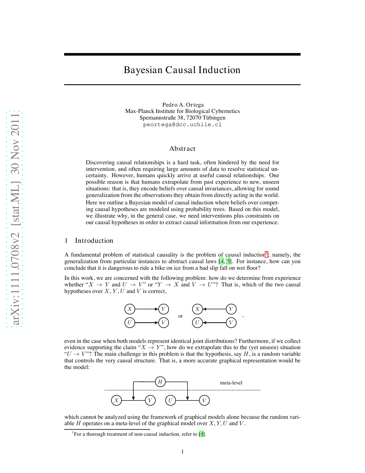
In this work, we are concerned with the following problem: how do we determine from experience whether “X → Y and U → V " or “Y → X and V → U “? That is, which of the two causal hypotheses over X, Y , U and V is correct, PSfrag replacements
even in the case when both models represent identical joint distributions? Furthermore, if we collect evidence supporting the claim “X → Y “, how do we extrapolate this to the (yet unseen) situation “U → V “? The main challenge in this problem is that the hypothesis, say H, is a random variable that controls the very causal structure. That is, a more accurate graphical representation would be the model:
which cannot be analyzed using the framework of graphical models alone because the random variable H operates on a meta-level of the graphical model over X, Y, U and V .
PSfrag replacements
A device with a green and a red light bulb. A switch allows controlling the state of the green light: either “on”, “off” or “undisturbed”. (Right) A second device having a green spinner and a red spinner, both of which can either lock into a horizontal or vertical position. The two devices are connected through a cable, establishing thus a relation among their randomizing mechanisms.
In this work these difficulties are overcome by using a probability tree to model the causal structure over the random events [9]. Probability trees can encode2 alternative causal realizations, and in particular alternative causal hypotheses. All random variables are of the same type-no distinctions between meta-levels are needed. Furthermore, we define interventions [7] on probability trees so as to predict the statistical behavior after manipulation. We then show that such a formalization leads to a probabilistic method for causal induction that is intuitively appealing.
Imagine we are given a device with two light bulbs, one green (X) and one red (Y ), whose states obey a hidden mechanism that correlates them positively. Moreover, the box has a switch that allows us controlling the state of the green bulb: we can either leave it undisturbed, or we can intercept the mechanism by turning the light on or off as we please (Figure 1, left device). We encode the “on” and “off” states of the green light as X = x and X = ¬x respectively. Analogously, Y = y and Y = ¬y denote the “on” and “off” states of the red light. We ponder the explanatory power of two competing hypotheses: either “green causes red” (H = h) or “red causes green” (H = ¬h).
Assume that the probabilities governing the realization of H, X and Y are as detailed in Figure 2a. In this tree, each (internal) node is interpreted as a causal mechanism; hence a path from the root node to one of the leaves corresponds to a particular sequential realization of causal mechanisms 3 . The logic underlying the structure of this tree is self-explanatory:
- Causal precedence: A node causally precedes its descendants. For instance, the root node corresponding to the sure event Ω causally precedes all other nodes.
Each node resolves the value of a random variable. For instance, given the node corresponding to H = h and X = ¬x, either Y = y will happen with probability P(y|h, ¬x) = 1 4 or Y = ¬y with probability P(¬y|h, ¬x) = 3 4 .
The resolution order of random variables can vary across different branches. For instance, X precedes Y under H = h, but Y precedes X under H = ¬h. This allows modeling different causal hypotheses.
While the probability tree represents our subjective model explaining the order in which the random values are resolved, it does not necessarily correspond to the temporal order in which the events are revealed to us. So for instance, under hypothesis H = h, the value of the variable Y might be revealed before X, even though X causally precedes Y ; and the hypothesis H, which precedes both X and Y , is never observed. b) The probability tree resulting from (a) after setting X = x.
Suppose we observe that both lights are on. Have we learned anything about their causal dependency? A brief calculation shows that this is not the case because the posterior probabilities are equal to the prior probabilities:
P(h|x, y) = P(y|h, x)P(x|h)P(h) P(y|h, x)P(x|h)P(h) + P(x|¬h, y)P(y|¬h)P(¬h)
This makes sense intuitively, because by just observing that the two lights are on, it is statistically impossible to tell which one caused the other. Note how the factorization of the likelihood P (x, y|H) depends on whether H = h or H = ¬h. How do we extract causal information then? To answer this question, we make use of a crucial insight of statistical causality:
To obtain new causal information from statistical data, old causal information needs to be supplied (paraphra
This content is AI-processed based on open access ArXiv data.