Topologically Robust CAD Model Generation for Structural Optimization
📝 Original Paper Info
- Title: Topologically robust CAD model generation for structural optimisation- ArXiv ID: 1906.07631
- Date: 2020-07-15
- Authors: Ge Yin, Xiao Xiao, Fehmi Cirak
📝 Abstract
Computer-aided design (CAD) models play a crucial role in the design, manufacturing and maintenance of products. Therefore, the mesh-based finite element descriptions common in structural optimisation must be first translated into CAD models. Currently, this can at best be performed semi-manually. We propose a fully automated and topologically accurate approach to synthesise a structurally-sound parametric CAD model from topology optimised finite element models. Our solution is to first convert the topology optimised structure into a spatial frame structure and then to regenerate it in a CAD system using standard constructive solid geometry (CSG) operations. The obtained parametric CAD models are compact, that is, have as few as possible geometric parameters, which makes them ideal for editing and further processing within a CAD system. The critical task of converting the topology optimised structure into an optimal spatial frame structure is accomplished in several steps. We first generate from the topology optimised voxel model a one-voxel-wide voxel chain model using a topology-preserving skeletonisation algorithm from digital topology. The weighted undirected graph defined by the voxel chain model yields a spatial frame structure after processing it with standard graph algorithms. Subsequently, we optimise the cross-sections and layout of the frame members to recover its optimality, which may have been compromised during the conversion process. At last, we generate the obtained frame structure in a CAD system by repeatedly combining primitive solids, like cylinders and spheres, using boolean operations. The resulting solid model is a boundary representation (B-Rep) consisting of trimmed non-uniform rational B-spline (NURBS) curves and surfaces.💡 Summary & Analysis
This paper proposes an automated and topologically accurate approach to convert a structurally optimized finite element model into a parametric CAD model. The process involves several key steps: 1. **Digital Topology and Skeletonization**: The structure from topology optimization is represented as a voxel model, which is then skeletonized using digital topology algorithms. This step focuses on analyzing the connectivity of all vertices in the voxel model to compute the Euler index. 2. **Skeletonization Algorithm**: The algorithm removes vertices without changing the topology, creating a 1-voxel wide chain model. 3. **Frame Structure Generation and Optimization**: The generated skeleton is transformed into a frame structure, which is then optimized for member size and layout to recover any lost efficiency during the optimization process. 4. **Reproduction in CAD System**: Finally, the frame structure is reproduced in a CAD system using basic solids like cylinders and spheres, combined repeatedly, resulting in a B-Rep model based on NURBS curves and surfaces.The key outcome of this approach is that it significantly reduces time and effort required for manual CAD modeling. The generated models are compact with minimal parameters, making them easy to edit and further process within the CAD system. This method offers substantial benefits by saving time and costs in product design and manufacturing processes, particularly for complex structures, allowing design teams to focus more on creative tasks.
📄 Full Paper Content (ArXiv Source)
The input to skeletonisation is a structured hexahedral finite element grid with all the vertices within the domain having eight incident hexahedra. For digital topology only the connectivity of the mesh is relevant whereas the coordinates of the grid nodes can be arbitrary so that in the following hexahedron and voxel are used interchangeably. The hexahedral grid encodes the binary voxel model of the topology optimised structure. The binary voxel model is obtained by denoting voxels with a density $`\rho_i`$ above the threshold $`\eta`$ as solid and the remaining ones as empty (void). Hence, the set of all voxels $`v \in \set V = \set V_s \cup \set V_e`$ is composed of the solid voxels $`\set V_s`$ and empty voxels $`\set V_e`$. Skeletonisation aims to reassign voxels one by one from $`\set V_s`$ to $`\set V_e`$ until the solid is represented by a network of one-voxel-wide chains. The decision about which voxels to reassign is guided by digital topology and proceeds starting from the voxels at the border between $`\set V_s`$ and $`\set V_e`$.
Review of digital topology
To retain the topology of the voxel model, its Euler characteristic is considered. The solid voxels in $`\set V_s`$ and empty voxels in $`\set V_e`$ yield two hexahedral volume meshes, or more abstractly cell complexes, which will be in the following denoted with $`\set M_s = \set M (\set V_s)`$ and $`\set M_e = \set M (\set V_e)`$. The volume mesh of a voxel set consists of the corresponding set of the vertices, edges, faces and voxels. It is also useful to define quadrilateral surface meshes $`\partial \set M_s`$ and $`\partial \set M_e`$ formed by the boundaries of $`\set M_s`$ and $`\set M_e`$, respectively. The Euler characteristic of the voxel model can be determined either from the volume mesh $`\set M_s`$ with
\begin{equation}
 \label{eq:eulerVol}
    \chi  (\set M_s) = n_0 (\set M_s)  - n_1 (\set M_s) + n_2 (\set M_s) - n_3 (\set M_s) \, ,
\end{equation}or from the surface mesh $`\partial \set M_s`$ with
\begin{equation}
 \label{eq:eulerSurf}
    \chi  (\partial \set M_s) = n_0 (\partial \set M_s) - n_1 (\partial \set M_s)+ n_2 (\partial \set M_s) \, ,
\end{equation}where $`n_0`$ denotes the number of vertices, $`n_1`$ the number of edges, $`n_2`$ the number of the faces and $`n_3`$ the number of hexahedrons in $`\set M_s`$ or $`\partial \set M_s`$. In Figure 1 the Euler characteristics of three voxel meshes are given. Notice that there is also the relation
\begin{equation}
    \chi(\partial \set M_s) = 2 \chi (\set M_s)
\end{equation}between the Euler characteristics of the surface and volume meshes. The Euler characteristic of a voxel model is related to the total number of separate objects (connected components) $`o(\set M_s)`$, handles (tunnels) $`h(\set M_s)`$ and cavities $`c(\set M_s)`$ in the entire model according to the formula
\begin{equation}
 \label{eq:eulerGlobal}
        \chi (\set M_s) = o(\set M_s) - h(\set M_s) + c(\set M_s) \, ,
\end{equation}see, e.g., textbooks on topology. For instance, the Euler characteristic $`\chi(\set M_s)`$ of a sphere is $`1`$, of a torus is $`0`$, of a double torus is $`-1`$ and so on, compare also Figure 1. Hence, the total number of different entities in the mesh and the described shape are intrinsically connected.
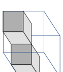
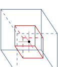
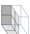
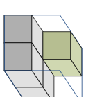
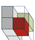
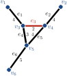
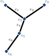
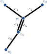
In determining the Euler characteristic of a voxel model, two different types of neighbourship definitions are possible, see Figure 2. These definitions define how pairs of touching voxels such as shown in Figure [fig:touchingVoxels_1] and [fig:touchingVoxels_2] are treated, whether connected and forming one surface or disconnected and forming two surfaces. That is, the number of entities in [eq:eulerVol] and [eq:eulerSurf] depends on the chosen definition of the neighbourship. For a voxel $`v`$ its 6-neighbours consist of all the cells which share a face with $`v`$ and its 26-neighbours consist of all the cells which share a common vertex with $`v`$. The voxels in the 6-neighbourhood of $`v`$ are denoted with $`\set N_{6}(v)`$ and the ones in the 26-neighbourhood with $`\set N_{26}(v)`$. In our implementation, two solid voxels are considered to be neighbours when they are 26-neighbours. In contrast, two void voxels are considered to be neighbours when they are 6-neighbours. As pointed out in Kong et al. , it is essential not to use the same neighbourship definitions for both the solid and void voxels. The use of one single neighbourhood definition leads to ambiguities, for instance, in the planar case to the violation of the Jordan curve theorem. The Jordan curve theorem states that a simple closed curve divides the plane into an interior and an exterior region.
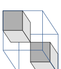
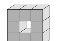
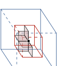
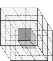
The Euler characteristic [eq:eulerVol] and [eq:eulerSurf] for the entire voxel model can be determined by looping over all vertices in the grid and only considering in each step the voxels attached to one vertex. The 2$`\times`$2$`\times`$2 voxels attached to a vertex $`q`$ are defined as its octant $`\set O(q)`$.1 There are as many octants as vertices in the volume grid (assuming that the voxel domain is padded with empty ghost voxels). The octants are overlapping and the edges, faces and voxels in the hexahedral mesh $`\set M_s`$ appear in several octants. Hence, in computing the Euler characteristic [eq:eulerVol] by iterating over the vertices the contribution of each octant has to be suitably weighted such that
\begin{equation}
  \label{eq:eulerSum}
    \chi (\set M_s) = \sum_q \chi (\set O(q)) = \sum_{q} \left  (1 -\frac{n_1^{(q)}}{2} + \frac{n_2^{(q)}} {4} -   \frac{n_3^{(q)}} {8} \right )  \, ,
\end{equation}where $`n_1^{(q)}`$ is the number of edges and $`n_2^{(q)}`$ is the number of faces neighbouring to the $`n_3^{(q)}`$ solid voxels in the mesh $`\set M(\set O(q)) \setminus \partial \set M(\set O(q))`$, see Figure 3. The contribution of an octant $`\chi(\set O(q))`$ with different solid-empty voxel states can be precomputed and stored in a look-up table. The eight voxels in an octant have $`2^8=256`$ possible solid-empty states and considering symmetries this reduces to only 22 distinct cases. Tables with contributions of octants to the Euler characteristic can be found, e.g., in
Skeletonisation by successive voxel removal
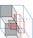
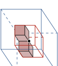
The Euler characteristic $`\chi (\set M_s)`$ is critical in determining the voxels at the boundary of the solid mesh $`\set M_s`$ that can be deleted without changing the topology of the voxel model. A solid border voxel is defined as a solid voxel with at least one void voxel amongst its 6-neighbours. There is a large amount of research on voxels, also referred to as simple points, which can be removed without changing topology . As evident from [eq:eulerGlobal] simply conserving the Euler characteristic $`\chi(\set M_s)`$ of the entire or a portion of the mesh does not ensure that the topology is not changed, i.e. the number of objects $`o(\set M_s)`$, handles $`h(\set M_s)`$ and cavities $`c(\set M_s)`$ all remain the same. For a solid border voxel $`v`$ to be classified as simple its removal must not change, in addition to the Euler characteristic, the number of objects and handles for both $`\set M_s`$ and $`\set M_e`$ . According to Lee et al. these conditions can be checked by examining the state of the voxels in eight octants overlapping voxel $`v`$, or the voxels in $`v`$’s 26-neighbourhood $`\set N_{26}(v)`$. That is, a border voxel $`v`$ is a simple point if and only if
\label{eq:changeCrit}
\begin{align}
    \Delta \chi  (\set M \left ( \set N_{26}(v))  \right )  &= 0 \quad  \text{ and }  \label{eq:changeChi}  \\
    \Delta h \left (\set M(\set N_{26}(v))  \right ) &= 0  \quad \text{ or }  \\
    \Delta o \left ( \set M(\set N_{26}(v))  \right ) &= 0  \label{eq:changeObj} \, ,
\end{align} \label{eq:simpleCheck}where $`\Delta`$ denotes the change of the respective quantity with and without voxel $`v`$ present. It is straightforward to determine the Euler characteristic [eq:changeChi] and it is relatively easy to determine the number of objects [eq:changeObj] in $`\set N_{26}(v)`$. The change of the Euler characteristic is determined by summing the tabulated contributions of the eight octants belonging to the eight corners of the voxel $`v`$ from , see [eq:eulerSum] and Figure 4. To determine the number of objects [eq:changeObj], we generate an undirected graph with the solid voxels as nodes and introducing edges between voxels that are 26-neighbours. Subsequently, the number of connected components is determined with a depth first search (DFS) algorithm .
The skeletonisation proceeds by removing in each step one layer of border voxels which are simple points according to [eq:simpleCheck], see Algorithm [alg:skeletonisation] in 18. The removed solid voxels are reclassified as void. One removal step is split into six sub-steps and in each sub-step only the voxels approaching from one of the six grid directions are removed. The geometry of the obtained skeleton depends somewhat on the sequencing of these sub-steps, which is not critical for our purpose. It is straightforward to tag some voxels as non-removable irrespective of [eq:simpleCheck]. In skeletonising topology optimisation results, for instance, the voxels at Dirichlet and non-zero Neumann boundaries are tagged as non-removable. Also, end points with only one voxel in their 26-neighbourhood have to be tagged as non-removable, in order to avoid a complete elimination of voxel chains. The skeletonisation terminates when none of the remaining voxels is removable without violating [eq:simpleCheck]. The final result is a curve skeleton consisting of a network of one-voxel-wide voxel chains connected by joint voxels. We refer to this curve skeleton as the voxel chain skeleton.
Illustrative example and timing
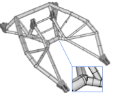
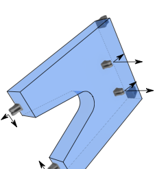
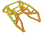
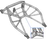
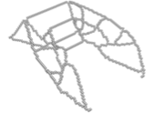
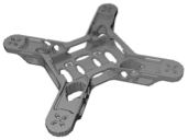
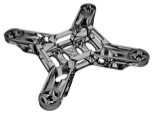
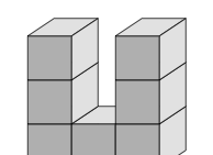
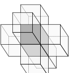
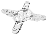
We consider the skeletonisation of the quadcopter frame shown in Figure [fig:quadCopter_model] obtained from GrabCAD. The frame has a non-trivial topology and has been designed in a CAD system. To generate a voxel model the implicit, or level set, representation of the frame on a uniform voxel grid is computed first. This is achieved by determining the distance of each voxel in the grid to the frame surface with the open source openVDB library . In doing so, the frame geometry is approximated with the STL mesh exported from the CAD system depicted in Figure [fig:quadCopter_stl]. After thresholding the voxel grid the voxel model of the frame in Figure [fig:quadCopter_voxel] is obtained. Its skeletonisation with the introduced digital topology algorithm yields the voxel chain skeleton in Figure [fig:quadCopter_skeleton]. It can be visually confirmed that the skeleton appears to have the same topology as the voxel model.
To investigate the efficiency and scaling of our C++ implementation of the introduced skeletonisation algorithm, we consider three different voxel grids for computing the implicit representation and skeletonisation. The size of the three grids, the number of voxels in the different models and the runtimes are given in Table 7. The STL mesh has in all cases 1086791 triangles. The number of solid voxels in the voxel model and the number of removal steps increase with decreasing voxel size because more and more of them cover the frame. The number of skeleton voxels increases because the smaller voxels can capture the topology of the frame better. The reported extremely short runtimes include only skeletonisation (no implicitisation) and confirm the efficiency of the skeletonisation algorithm. Moreover, notice that the average time per removal step is approximately linear with respect to the number of the voxels in the voxel grid. The experiments were performed on a Macbook Pro with an Intel Core CPU i7-4750HQ $`@`$ 2.0GHz and 16GB RAM.
|
|
|
|
|
| ||||||||||
|---|---|---|---|---|---|---|---|---|---|---|---|---|---|---|---|
| Grid 1 | 139 × 16 × 139 | 18222 | 1278 | 4 | $\phantom{0}4.43$ s | 17.73 s | |||||||||
| Grid 2 | 172 × 19 × 172 | 38076 | 1677 | 5 | $\phantom{0}9.33$ s | 46.65 s | |||||||||
| Grid 3 | 197 × 21 × 197 | 53981 | 1894 | 6 | 13.17 s | 78.99 s |
Examples
We consider three examples of increasing complexity to demonstrate the application of the proposed approach. The minimised cost function is the compliance $`J(\hat{\vec \rho})`$ in topology optimisation and $`J(\vec d, \, \vec x)`$ in size and layout optimisation, where $`\hat{\vec \rho}`$ are the filtered element densities, $`\vec d`$ are the member diameters, and $`\vec x`$ are the joint coordinates. In all examples, the Young’s modulus and Poisson’s ratio of the solid material are $`\overline E=2.1 \cdot 10^5`$ and $`\nu=0.3`$. In topology optimisation the penalisation factor is chosen as $`p = 3`$ and the minimum Young’s modulus as $`E_{min}=10^{-9}`$. During layout optimisation, a member shorter than $`1/20`$ of the total length of its immediate neighbouring members is considered as too short, and its two end nodes are merged.
Cantilever
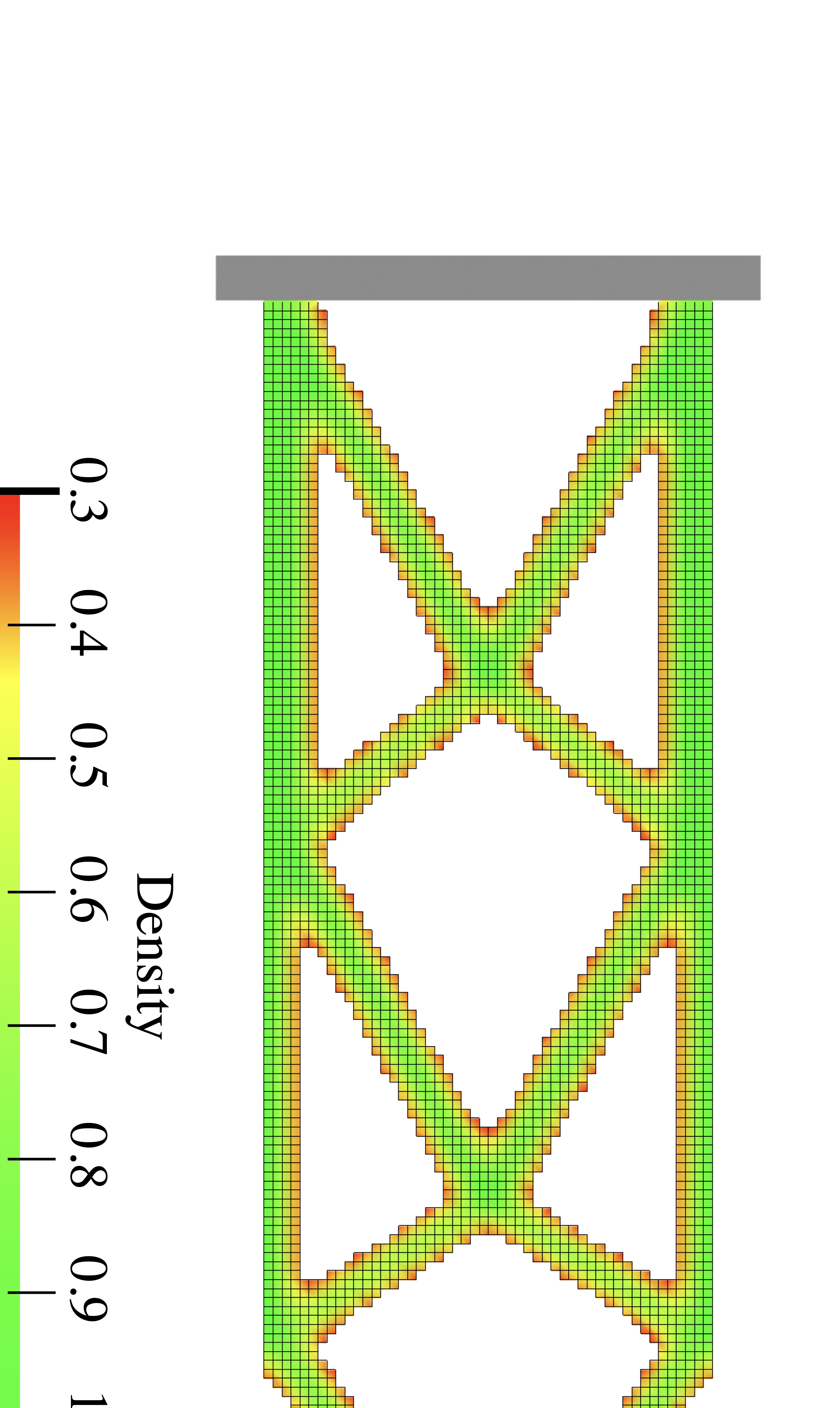
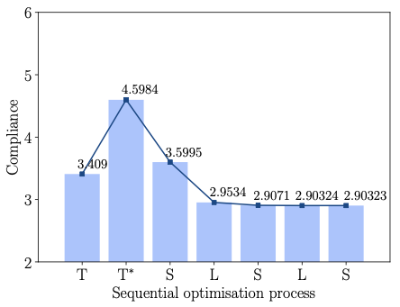
Cantilevered plates as shown in Figure 6 are one of the most widely studied benchmark examples in topology optimisation, see e.g. . The length, height and width of the chosen design domain are $`150 \times 50 \times 4`$. The left face of the domain is clamped while all the other faces are free, and a distributed force with a total value of $`F = 100`$ is applied along the centre of the right face. The finite element discretisation consists of $`150 \times 50 \times 4`$ linear hexahedral elements. The maximum volume fraction of the optimised structure is prescribed to be $`V_f = 0.3`$ and the density filter radius is chosen as $`R=3`$. Figure [fig:cantilever_top] depicts the optimised cantilever with only the voxels above a relative density $`\eta=0.3`$. The compliance of this voxel model is $`J(\hat{\vec \rho})=3.40900`$, which has been determined after topology optimisation by resetting $`p=1`$ in [eq:younPenalised].
 style="width:47.5%" />
As a first step in obtaining the structural frame model the homotopic skeletonisation algorithm is employed. The skeletonisation yields after $`5\times6`$ voxel removal steps the voxel chain skeleton shown in Figure [fig:cantilever_skeleton]. As visually apparent, the voxel and voxel chain models have the same topology. The skeleton is converted into the structure depicted in Figure [fig:cantilever_frame] by first identifying the 16 joints and then connecting them with 21 members. As evident from Figure [fig:cantilever_frame] during the conversion to a frame model the optimality of the voxel model is compromised; note, for instance, the non-straight top and bottom members. Optimality is recovered by updating the joint positions, i.e. layout optimisation, and the cross-sectional areas, i.e. size optimisation, see Figure [fig:cantilever_result]. Initially, all members are assumed to have the same diameter of $`d=4.547`$, giving the prescribed total volume of $`V = 0.3 \overline V`$. In determining the volume only the member cross-sections and member lengths between the joints are considered.
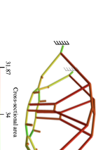
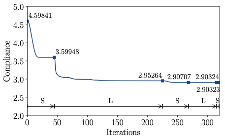
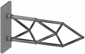
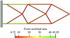
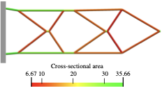
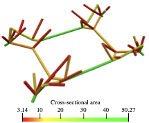
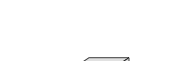
According to Figure [fig:cantilever_conv_frame], the frame consisting of beams with uniform diameter has a compliance $`J(\vec d, \vec x) = 4.59841`$, which is larger than the voxel model. The stretch and bending strain energies of the frame are 2.02202 and 0.247108, respectively. The minimum and maximum axial stresses are 0 and 20.9274. The average axial stress is 8.04859 and its standard deviation is 6.26102. After the first size optimisation step the compliance is reduced to $`J(\vec d, \, \vec x) = 3.59948`$ and the subsequent layout optimisation step to $`J(\vec d, \, \vec x)=2.95264`$. Several more steps of size and layout optimisation do not lead to a significant reduction in the compliance. Notice that the obtained final compliance $`J(\vec d, \, \vec x) = 2.90323`$ is significantly lower than the compliance $`J(\hat{\vec \rho})= 3.40900`$ of the topology optimised voxel model. The stretch and bending strain energies of the final frame are 1.42114 and 0.0190822, respectively. The minimum and maximum axial stresses are 7.00854 and 8.46234. The average axial stress is 8.09638 and its standard deviation is 0.44709. In the final optimised cantilever in Figure [fig:cantilever_result] the axial stresses become more evenly distributed and the bending stresses are significantly reduced. The final optimised cantilever consists of 11 joints and 16 members. Finally, in Figure 8 the solid CAD model of the frame and a faceted triangular STL mesh exported from FreeCAD are shown. The lines in the CAD model show the layout of the trimmed NURBS patches.
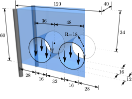
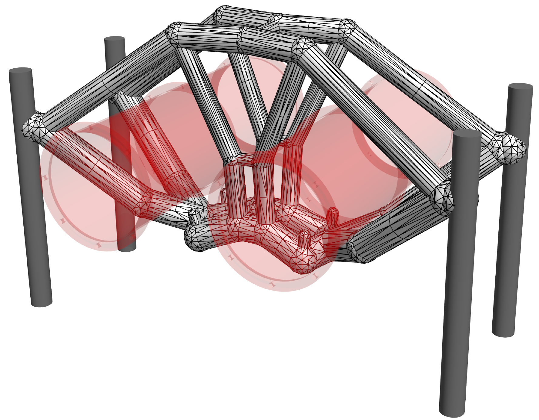
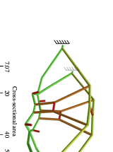
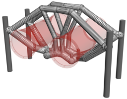
Pipe bracket
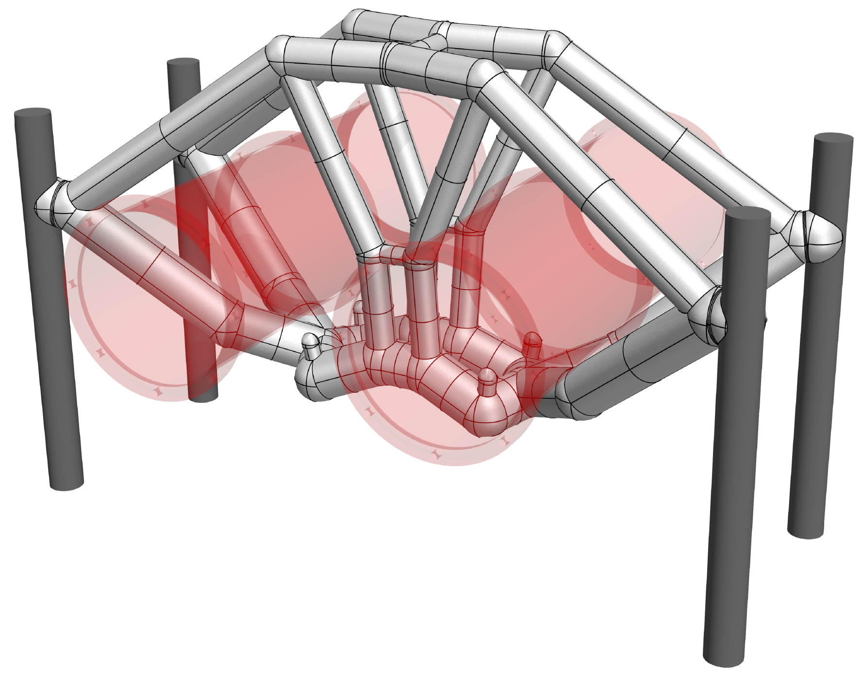
As a structure with a truly three-dimensional load path, the pipe bracket shown in Figure 9 is considered. The design domain has a length, height and width of $`120 \times 40 \times 60`$ and contains two openings with each of radius of 18 for two pipes passing through the domain. Within the openings each pipe is supported at four points, applying at each support a vertical force of $`F=100`$. The four vertical outer edges of the design domain are chosen as fixed. The finite element discretisation consists of $`120 \times 40 \times 60`$ linear hexahedral elements. To represent the two openings in the finite element model the Young’s modulus of the elements within the void region is prescribed with $`E_{\text{min}}`$.
 style="width:47.5%" />
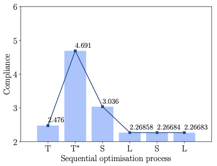
The maximum volume fraction of the optimised structure is prescribed to be $`V_f = 0.1`$ and the density filter radius is chosen as $`R = 3`$. Figure [fig:pipe_top] depicts the optimised bracket with only the voxels above a relative density $`\eta=0.5`$. The compliance of the optimised voxel model is $`J(\hat{\vec \rho})=2.47602`$. As easily recognisable from Figure [fig:pipe_top], the optimised structure is a combination of an arch-like and a cable-like structure with vertical tension members between the two openings.
The skeletonisation algorithm yields after $`6\times6`$ voxel removal steps the voxel chain skeleton in Figure [fig:pipe_skeleton]. The skeleton is converted into the structure depicted in Figure [fig:pipe_frame] by first identifying the 42 joints and then connecting them with 50 straight members. Alternatively, the 50 members can be represented with curved Bézier segments, which would lead to a structural frame with curved beam members. This has not been pursued here because such members may lead to an increase in manufacturing costs and are usually not preferred. Initially, all frame members are assumed to have the same diameter $`d=6.296`$, giving a total volume of $`V = 0.1 \overline V`$.
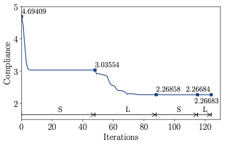
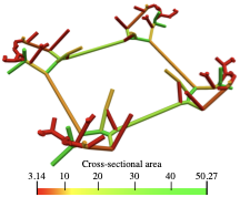
According to Figure [fig:pipe_conv_frame], the frame with beams of uniform diameter has a compliance $`J(\vec d, \, \vec x) = 4.69409`$, which is significantly higher than $`J(\hat{\vec \rho})=2.47602`$ of the voxel model. After the first size optimisation step the compliance is reduced to $`J(\vec d, \,\vec x) = 3.03554`$ and the subsequent layout optimisation step to $`J(\vec d, \, \vec x)=2.26858`$. In layout optimisation the beams are constrained not to move inside the volume occupied by the two cylindrical pipes. The intersection between a beam and a cylinder is determined by integrating the (positive) signed distance of the cylinder along the beam. It is straightforward to differentiate this constraint integral with respect to nodal coordinates of the beam. The intersection constraints for all the beams are aggregated with the Kreisselmeier-Steinhauser (K-S) function . Several more steps of size and layout optimisation do not lead to a significant reduction in the cost function. Notice that the obtained final compliance $`J(\vec d, \, \vec x)= 2.26683`$ is lower than the compliance $`J(\hat {\vec \rho})=2.47602`$ of the topology optimised voxel model. The final optimised frame structure depicted in Figure [fig:pipe_result] consists of 36 joints and 44 members. In Figure 11 the solid CAD model of the pipe bracket and a faceted triangular STL mesh exported from FreeCAD are shown.
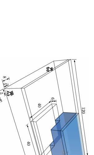
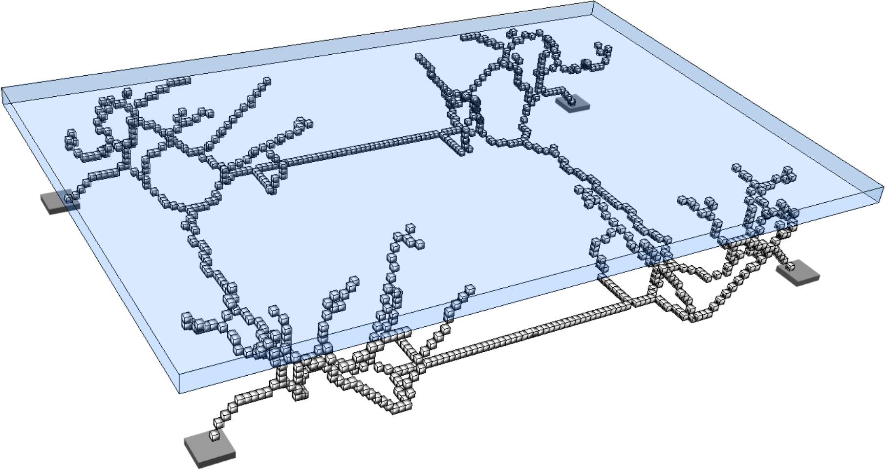
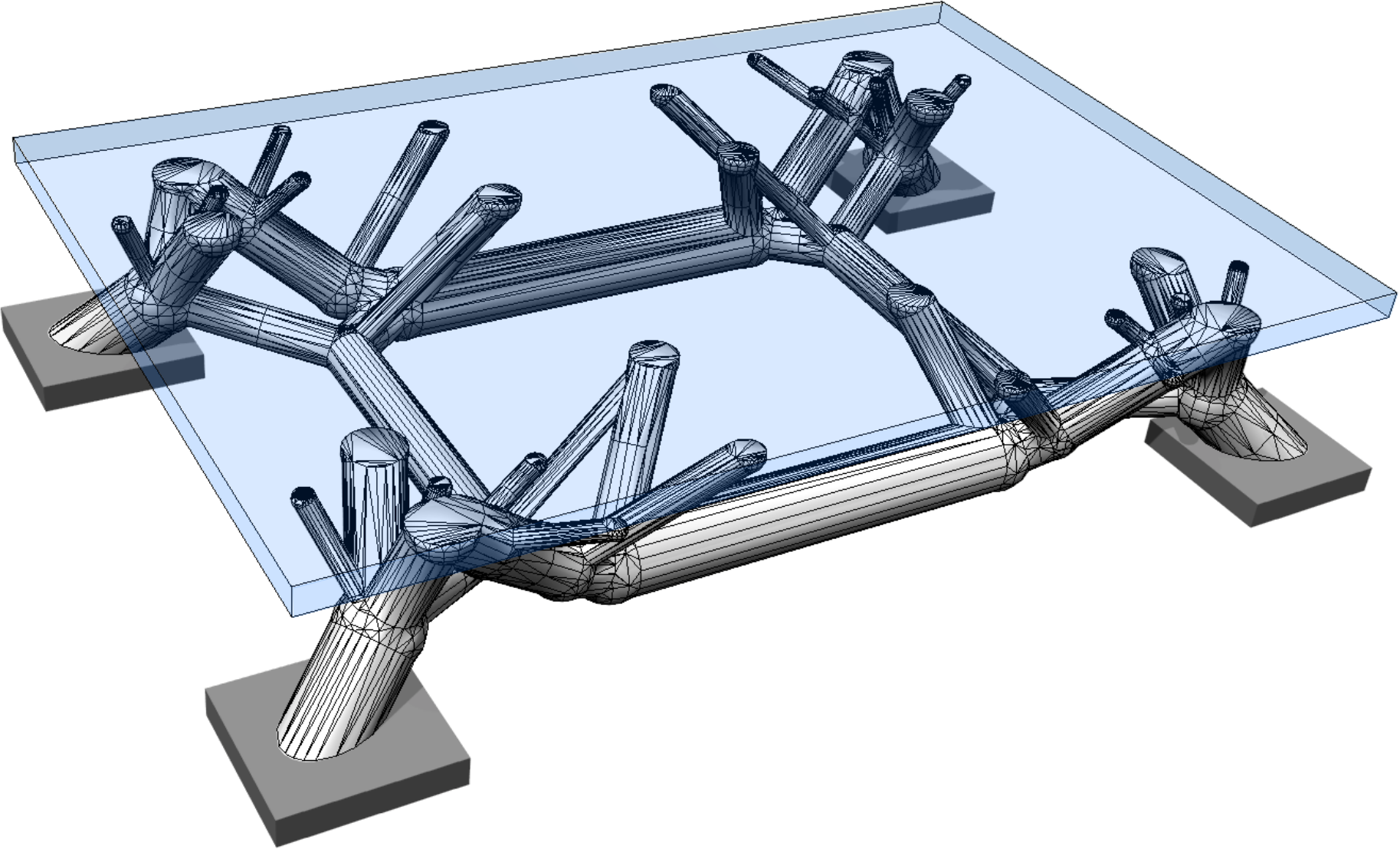
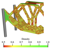
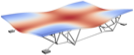
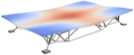
Frame-supported plate
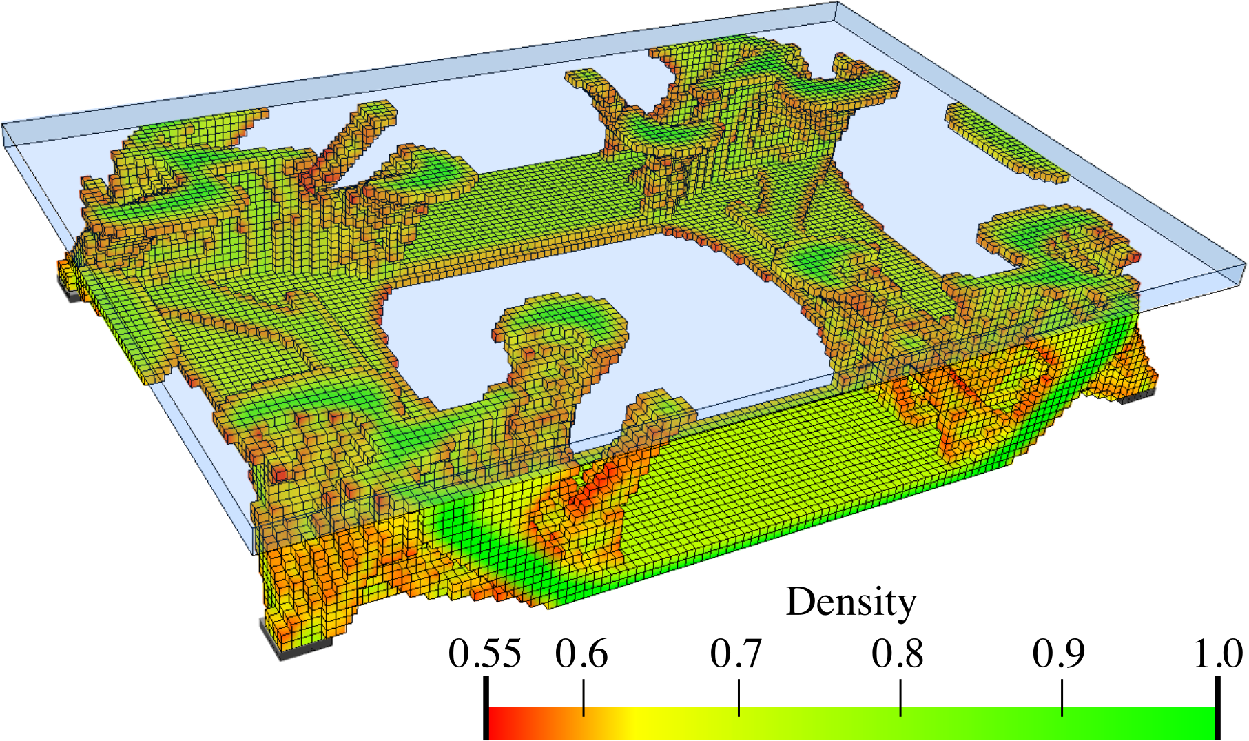
In structural design it is very common to combine a plate- or shell-like skin structure with a frame-like support structure. In such composite structures the skin can be modelled as a standard plate or shell structure, and topology optimisation is applied only in the remaining part of the design domain. The design domain shown in Figure 12 combines a thin plate-like skin with a solid bottom part to be optimised. The entire domain is of size $`120 \times 80 \times 20`$ and contains a small opening of size $`40 \times 40 \times 6`$. The plate is of thickness $`3`$ and is subjected to a uniform pressure load of $`1`$. The four corners of the design domain are vertically supported. Due to symmetry only a quarter of the design domain is considered in topology optimisation. The finite element discretisation consists of $`60 \times 40 \times 23`$ linear hexahedral finite elements. Across the height of the design domain there are $`6`$ elements with a size of $`1\times1\times0.5`$ in the plate-like top part and $`17`$ unit sized elements in the bottom part. To represent the small opening in the finite element model the Young’s modulus of the relevant elements is prescribed as $`E_\text{min}`$.
 style="width:47.5%" />
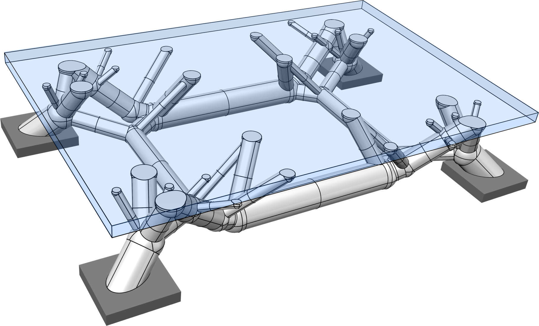
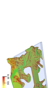
In topology optimisation, the maximum volume fraction is prescribed to be $`V_f = 0.25`$ and the density filter radius is chosen as $`R = 1.5`$. The optimised structure with only the voxels above a relative density $`\eta = 0.55`$ is shown in Figure [fig:deck_top] and its voxel chain skeleton in Figure [fig:deck_skeleton]. Although the voxels in the top part of the design domain are present during optimisation and skeletonisation, they are tagged as non-removable. The voxel chain skeleton is converted to the frame structure shown in Figure [fig:deck_frame]. The structural model also contains a top plate not shown in Figure [fig:sizeLayoutOptimised]. The plate is modelled as a Kirchhoff–Love plate and is discretised with $`4\times4`$ quadrilateral elements and Catmull-Clark subdivision basis functions. The frame has 124 joints and 136 members. Initially, all the members are assumed to have the same diameter of $`d=5.010`$ which gives a total frame volume of $`V = 4800`$. The coupling between the plate and the frame is achieved with Lagrange multipliers as described in . The joints between the plate and frame can transfer forces but not moments.
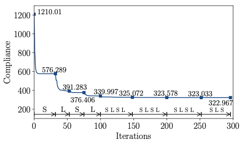
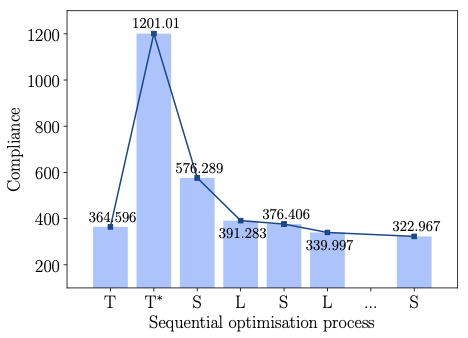
According to Figure [fig:deck_conv_frame], the compliance of the frame-supported plate with members of uniform diameter is $`J(\vec d, \, \vec x) =1210.01`$, which reduces after several sequential size and layout optimisation steps to $`J(\vec d, \, \vec x) =322.967`$. During the layout optimisation, the positions of the joints between the frame and plate are fixed. For comparison, the compliance of the topology optimised voxel model was $`J(\hat{\vec \rho})=364.596`$. The final optimised frame structure contains 56 joints and 64 members, see Figure [fig:deck_result]. Its solid CAD model and faceted triangular STL mesh exported from FreeCAD are depicted in Figure 13.
Overall optimisation and conversion process
In this Section, we review the sequence of steps from the definition of the topology optimisation problem to obtaining the structurally-sound parametric CAD geometry. We provide additional details for each of the steps and focus on the interplay between the different steps. Each step corresponds to one Section in this paper.
Step 1: Topology optimisation
We assume that the finite element mesh for the optimisation problem [eq:topOpt] is a structured hexahedral grid. In most optimisation problems, the design domain is a parallelepiped which can be discretised with a structured grid. Other more complex design domains can be considered by computing their implicit, or level set, representation and embedding them in a structured hexahedral grid, see the quadcopter frame example in Figure 5. From the outset, the voxels outside the design domain are chosen as void by choosing their Young’s moduli with $`E_{\text{min}}`$.
Step 2: Skeletonisation
The input to the homotopic skeletonisation algorithm is a binary image defined on a hexahedral structured grid. The binary image is obtained by thresholding the topology optimised geometry. The threshold value $`\eta`$ is chosen such that the prescribed material volume constraint [eq:topOptC] in topology optimisation is retained. The output of the skeletonisation is a curve skeleton in the form of a voxel chain with the same topology as the topology optimised geometry.
Step 3: Structural frame model generation
The topology and joint coordinates of the frame model are extracted from the voxel chain model. It is assumed that all the members are straight, have a circular cross-section with the same diameter and their total volume is equal to the prescribed material volume $`V_f \overline{V}`$ in topology optimisation. It is possible to obtain frame models with more complex member geometries and non-uniform cross-sections. This appears to be, however, usually not desired from an ease and cost of manufacturability viewpoint.
Step 4: Size and layout optimisation
The structural frame model extracted from the skeleton is usually suboptimal. That is, the compliance of the structural frame is larger than the compliance of the topology optimised geometry. To recover the optimality of the frame structure, we apply several steps of sequential size and layout optimisation [eq:frameOpt]. In size optimisation the diameters $`d_i`$ of the circular member cross-sections and in layout optimisation the coordinates $`\vec x_i`$ of the joints are updated. Both optimisation problems are solved with the SQP (sequential quadratic programming) method . Throughout optimisation the volume of the frame is constrained to be equal to the prescribed material volume in topology optimisation $`V_f \overline{V}`$. It is straightforward to consider additional constraints pertaining to the member cross-sections, the positions of the joints, or positions and orientations of the members. The first step is always size optimisation, which is followed by as many as necessary alternating layout and size optimisation steps until the compliance cost function is converged. If the length of any member reduces to zero during shape optimisation, the member is removed, its end nodes are merged, and the iteration continues.
Step 5: CAD model generation
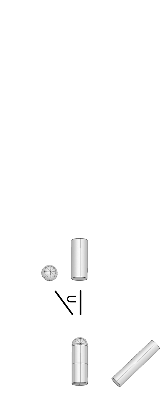
A compact CAD model of the structural frame can be generated essentially in any parametric CAD system using a fully automated process. The members are represented by cylinders and the joints by spheres which are combined by boolean operations. The underlying binary CSG tree representation makes it easy to edit further and to refine the optimised design.
Review of structural optimisation
In this Section, we briefly review the standard density based topology optimisation using the SIMP method and the size and layout optimisation of spatial frame structures. In all cases, the cost function is the compliance, and the discussion is restricted to aspects relevant to this paper. For further details see, e.g., the monographs .
Topology optimisation of solids
The topology optimisation problem for finite element discretised solids reads
\label{eq:topOpt}
\begin{align}
    \text{minimise } \quad  & J( \vec \rho) = \vec f \cdot \vec u (\vec \rho)  \label{eq:topOptA}\\
    \text{subject to} \quad  & \vec K (\vec \rho) \vec u  = \vec f  \label{eq:topOptB}\\
    & \frac{V(\vec \rho)}{\overline V} \le V_f \label{eq:topOptC} \\
    & \vec 0 \le \vec \rho \le  \vec 1  \, ,
\end{align}where $`J(\vec \rho)`$ is the compliance cost function, is the vector of relative element densities, $`\vec{u}`$ is the displacement vector, $`\vec K`$ is the global stiffness matrix, is the global external force vector, $`V(\vec \rho)`$ is the material volume, $`\overline V`$ is the design domain volume and $`V_f`$ is the scalar prescribed volume fraction. The relative density of each element is constrained to be $`0 \le \rho_i \le 1`$ with $`i \in \{1, \dotsc, n_e \}`$ and the number of elements is $`n_e`$.
As usual, the global stiffness matrix $`\vec K`$ and vector are assembled from the $`n_e`$ element contributions $`\vec K_i`$ and $`\vec f_i`$ in the mesh. In this paper, we discretise the design domain always with a structured grid and hexahedral linear elements. In each element $`i`$ the material is isotropic and homogeneous, and the Young’s modulus $`E`$ is penalised depending on the relative density $`\rho_i`$ with
\begin{equation}
 \label{eq:younPenalised}
    E  (\rho_i) = E_{\text{min}} + \rho_i^p (\overline{E}- E_{\text{min}}) \, ,
\end{equation}where $`\overline{E}`$ is the prescribed Young’s modulus of the solid material, $`p`$ and $`E_{\text{min}}`$ are two algorithmic parameters. The penalisation parameter $`p \ge 3`$ ensures that elements with densities close to $`\rho_i = 0`$ (void) and $`\rho_i = 1`$ (solid) are preferred. The small Young’s modulus $`E_{\text{min}} \approx 10^{-9}`$ of the void material prevents ill-conditioning of the global stiffness matrix when $`\rho_i = 0`$. Each element stiffness matrix $`\vec K_i`$ is computed using the corresponding Young’s modulus $`E(\rho_i)`$ with the relative density $`\rho_i`$, which is constant within an element.
Furthermore, the topology optimisation problem [eq:topOpt] is regularised by filtering the element densities $`\rho_i`$ to prevent checker-board instabilities and mesh dependency of the solution. This is accomplished by convolving the element densities with the kernel function
\begin{equation}
    H(\vec x_i, \, \vec x_j) =
    \begin{cases}
        R - \text{dist}(\vec x_i, \, \vec x_j)  &  \text{if} \, \,   \text{dist } (\vec x_i, \,  \vec x_j) \le R  \\
        0 &  \quad \text{else}
        \end{cases} \, ,
\end{equation}which depends on the coordinates of the centroids $`\vec x_i`$ and $`\vec x_j`$ of the elements $`i`$ and $`j`$, and the prescribed filter length $`R`$. With $`H(\vec x_i,\, \vec x_j)`$ at hand the filtered densities are given by
\begin{equation}
 \label{eq:filter}
    \hat \rho_i  = \frac{\sum_j H (\vec x_i, \, \vec x_j)   \rho_j} { \sum_j H (\vec x_i, \, \vec x_j)  }
\end{equation}assuming that all elements have the same volume.
For gradient-based optimisation the derivatives of the cost and constraint functions in [eq:topOpt] with respect to the relative densities $`\rho_i`$ are needed. In the following the relative densities $`\rho_i`$ in the topology optimisation problem [eq:topOpt] are replaced with the filtered relative densities $`\hat {\rho}_i`$. The derivative, or sensitivity, of the compliance cost function [eq:topOptA] reads
\begin{equation}
 \label{eq:sensitivity}
    \frac{\partial J (\hat {\vec \rho})}{ \partial  \rho_i} =  \sum_j  \vec f \cdot \frac{\partial \vec u  (\hat{\vec \rho}) }{\partial \hat \rho_j} \frac{\partial \hat {\rho}_j}{\partial \rho_i} \, .
\end{equation}Differentiating and rearranging the equilibrium constraint [eq:topOptB] gives
\begin{equation}
    \frac{\partial \vec u (\hat{\vec \rho})}{\partial \hat \rho_j} = -  \vec K^{-1}(\hat {\vec \rho}) \frac{\partial \vec K (\hat {\vec \rho})}{\partial \hat \rho_j} \vec u (\hat{\vec \rho})
\end{equation}and the derivative of the filtered densities [eq:filter] is
\begin{equation}
    \frac{\partial \hat \rho_j}{\partial \rho_i} =  \frac{H (\vec x_j , \vec x_i)}{\sum_k H (\vec x_j, \, \vec x_k)}  \, .
\end{equation}Introducing both derivatives into [eq:sensitivity] yields
\begin{equation}
 \label{eq:sensitivity2}
    \frac{\partial J (\hat {\vec \rho})}{ \partial  \rho_i} = - \sum_j  \vec u (\hat{\vec \rho})  \cdot \frac{\partial \vec K (\hat {\vec \rho})}{\partial \hat \rho_j} \vec u (\hat{\vec \rho}) \frac{H (\vec x_j , \vec x_i)}{\sum_k H (\vec x_j, \, \vec x_k)}     \, ,
\end{equation}where the stiffness matrix derivative is to be assembled from element contributions considering the penalised Young’s modulus [eq:younPenalised].
The derivative of the volume constraint [eq:topOptC] is obtained analogously with
\begin{equation}
 \label{eq:volSensitivity}
    \frac{\partial V (\hat {\vec \rho})}{ \partial  \rho_i} = \sum_j \hat \rho_j \frac{V}{n_e} \frac{H (\vec x_j , \vec x_i)}{\sum_k H (\vec x_j, \, \vec x_k)}     \, .
\end{equation}It is assumed here that all the elements are of the same size, namely the design volume $`\overline V`$ divided by the total number of elements $`n_e`$.
Finally, with the obtained derivative of the compliance cost function [eq:sensitivity2] and the volume constraint [eq:volSensitivity] the optimised density distribution is determined iteratively with the optimality criteria method, see e.g. .
Size and layout optimisation of frames
We consider spatial frame structures consisting of straight beam members connected by joints that can transfer forces and moments. The members can deform by stretching, bending and torsion and are modelled as classical Timoshenko beams, see 17. Without loss of generality, size and layout optimisation can be posed as an iterative sequential optimisation problem. In each optimisation step, either the size, i.e. cross-section area, or layout, i.e. joint coordinates, of the members is optimised.
Both the size and layout optimisation problems have the same structure as topology optimisation [eq:topOpt], namely,
\label{eq:frameOpt}
\begin{align}
    \text{minimise } \quad  & J(\vec s) = \vec u(\vec s) \cdot \vec K(\vec s) \vec u (\vec s) = \vec f \cdot \vec u (\vec s) \label{eq:frameOptA}\\
    \text{subject to} \quad  & \vec K (\vec s) \vec u (\vec s) = \vec f  \label{eq:frameOptB}\\
    & \frac{V(\vec s)}{\overline V} \le V_f \label{eq:frameOptC} \\
    & \vec s_l \le \vec s \le  \vec s_u  \, .
\end{align}The vector of design variables $`\vec{s}`$ refers either to cross-section areas in case of size optimisation or joint coordinates in case of layout optimisation. The two bounds $`\vec s_l`$ and $`\vec s_u`$ have different interpretations in the two cases.
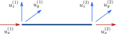
The frame consists of $`n_e`$ beam elements with the element stiffness matrices $`\vec K_i`$ and vectors $`\vec f_i`$. Each stiffness matrix $`\vec K_i`$ is obtained from a local stiffness matrix $`\vec K_i^l`$ formulated in a coordinate system attached to the element with the index $`i`$. The local matrix $`\vec K_i^l \in \mathbb R^{12 \times 12}`$ with the displacements and rotations of the two end nodes of the beam element as degrees of freedom is given in 17. In the local $`x^l_i`$, $`y^l_i`$ and $`z^l_i`$ coordinate system the beam axis is assumed to be aligned with the $`x^l_i`$ axis. The matrix $`K_i^l`$ is transformed to the global $`x`$, $`y`$ and $`z`$ coordinate system according to
\begin{equation}
 \label{eq:elmStiffness}
    \vec{K}_i = \vec{\Lambda}_i  \vec{K}_i^l \vec{\Lambda}_i^\trans
\end{equation}with the block-diagonal transformation matrix
\begin{equation}
    \vec{\Lambda}_i = \diag ( \vec{\lambda}_i, \, \vec{\lambda}_i,  \, \vec{\lambda}_i,  \, \vec{\lambda}_i )\, .
\end{equation}The rotation matrix $`\vec \lambda_i \in \mathbb R^{3\times3}`$ can be chosen with
\begin{equation}
    \vec{\lambda}_i =
    \begin{pmatrix}
        \cos\alpha_i \cos \beta_i & -\sin \alpha_i  & \cos \alpha_i \sin \beta_i   \\
        \sin\alpha_i \cos \beta_i  & \phantom{+} \cos \alpha_i & \sin \alpha_i \sin \beta_i  \\
        - \sin \beta_i  &
        0 & \cos \beta_i
    \end{pmatrix} \, ,
\end{equation}which is composed of the two elemental rotations $`\alpha_i`$ around the $`z_i^l`$ axis and $`\beta_i`$ around $`y_i^l`$ axis.
Similar as in topology optimisation, the derivative, or sensitivity, of the compliance cost function [eq:frameOptA] reads
\begin{equation}
 \label{eq:complianceDerivatives}
\frac{\partial J(\vec{s})}{\partial s_i} =
-\vec{u} (\vec{s}) \cdot \frac{\partial\vec{K}(\vec{s})}{\partial s_i}\vec{u}(\vec{s}) =  -\sum_{j = 1}^{n_e}\vec{u}_j (\vec{s}) \cdot \frac{\partial\vec{K}_j (\vec{s})}{\partial s_i}\vec{u}_j (\vec{s}) \, ,
\end{equation}where $`\vec{u}_j`$ is the vector of nodal displacements and rotations of the element $`j`$. In size optimisation the derivative of the element stiffness matrix [eq:elmStiffness] is given by
\begin{equation}
\frac{\partial \vec{K}_i(\vec{s})}{\partial s_j} = \vec{\Lambda}_i \frac{\partial{\vec{K}}_i^l}{\partial s_j}\vec{\Lambda}_i^\trans \, ,
\end{equation}whereas in layout optimisation it is
\begin{equation}
\frac{\partial \vec{K}_i(\vec{s})}{\partial s_j} =
\frac{\partial\vec{\Lambda}_i}{\partial s_j}  \vec K_i^l \vec{\Lambda}_i^\trans +
\vec{\Lambda}_i \frac{\partial \vec K_i^l}{\partial s_j}\vec{\Lambda}_i^\trans +
\vec{\Lambda}_i  \vec K_i^l \frac{\partial\vec{\Lambda}_i^\trans}{\partial s_j} \, .
\end{equation}📊 논문 시각자료 (Figures)


A Note of Gratitude
The copyright of this content belongs to the respective researchers. We deeply appreciate their hard work and contribution to the advancement of human civilization.Note that it is also possible to associate the octants with the voxels instead of the vertices in the grid. Both viewpoints are equivalent . ↩︎