In this section, we provide necessary background about generative models and variational autoencoders in particular.

Suppose we are given a set of data points $`X=\{x_1, \ldots, x_n\}`$ that are distributed according to some unknown probability distribution $`P(X)`$. Generative models seek to learn an approximate probability distribution $`Q`$ such that $`Q`$ is very similar to $`P`$. Most generative models also allow one to generate samples $`X'=\{x'_1, \ldots, \}`$ from the model $`Q`$ such that the $`X'`$ has similar statistical properties to $`X`$. Deep generative models use powerful function approximators (typically, deep neural networks) for learning to approximate the distribution.

VAEs are a class of generative models  that can model various complicated data distributions and generate samples. They are very efficient to train, have an interpretable latent space and could be adapted effectively to different domains such as images, text and music. Latent variables are an intermediate data representation that captures data characteristics used for generative modelling. Let $`X`$ be the relational data that we wish to model and $`z`$ a latent variable. Then $`P(X|z)`$ is the distribution of generating data given latent variable. We can model $`P(X)`$ in relation to $`z`$ as $`P(X)=\int P(X|z)P(z)dz`$ marginalizing $`z`$ out of the joint probability $`P(X,z)`$. The challenge is that we do not know $`P(z)`$ and $`P(X|z)`$. The underlying idea in variational modelling is to infer $`P(z)`$ using $`P(z|X)`$.

We use a method called Variational Inference (VI) to infer $`P(z|X)`$ in VAE. The main idea of VI is to approach inference as an optimization problem. We model the true distribution $`P(z|X)`$ using a simpler distribution (denoted as $`Q`$) that is easy to evaluate, e.g. Gaussian, and minimize the difference between those two distribution using KL divergence metric, which tells us how different $`P`$ is from $`Q`$. Assume we wish to infer $`P(z|X)`$ using $`Q(z|X)`$. The KL divergence is specified as:

\begin{equation}
\begin{split}
D_{KL}[Q(z|X)||P(z|X)]=\sum_{z}Q(z|X)\log(\frac{Q(z|X)}{P(z|X)}) = \\
E[\log(\frac{Q(z|X)}{P(z|X)})]=E[\log(Q(z|X)) - \log(P(z|X))]
\end{split}
\end{equation}

We can connect  $`Q(z|X)`$ which is a projection of the data into the latent space and $`P(X|z)`$ which generates data given a latent variable $`z`$ through Equation [eq:var2] that is also called as the variational objective.

\begin{equation}
\label{eq:var2}
\begin{split}
    \log P(X)-D_{KL}[Q(z|X||P(z|X)] \\ =E[\log P(X|z)]-D_{KL}[Q(z|X||P(z)]
    \end{split}
\end{equation}

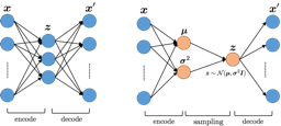
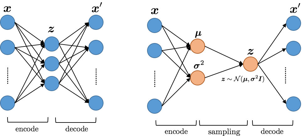
A different way to think of this equation is as $`Q(z|X)`$ encoding the data using $`z`$ as an intermediate data representation and $`P(X|z)`$ generates data given a latent variable $`z`$. Typically $`Q(z|X)`$ is implemented with a neural network mapping the underlying data space into the latent space (encoder network). Similarly $`P(X|z)`$ is implemented with a neural network and is responsible to generate data following the distribution $`P(X)`$ given sample latent variables $`z`$ from the latent space (decoder network). The variational objective has a very natural interpretation. We wish to model our data $`P(X)`$ under some error function $`D_{KL}[Q(z|X||P(z|X)]`$. In other words, VAE tries to identify the lower bound of $`\log(P(X))`$, which in practice is good enough as trying to determine the exact distribution is often intractable. For this we aim to maximize over some mapping from latent variables to $`\log P(X|z)`$ and minimize the difference between our simple distribution $`Q(z|X)`$ and the true latent distribution $`P(z)`$. Since we need to sample from $`P(z)`$ in VAE typically one chooses a simple distribution to sample from such as $`N(0,1)`$. Since we wish to minimize the distance between $`Q(z|X)`$ and $`P(z)`$ in VAE one typically assumes that $`Q(z|X)`$ is also normal with mean $`\mu(X)`$ and variance $`\Sigma(X)`$. Both the encoder and the decoder networks are trained end-to-end. After training, data can be generated by sampling $`z`$ from a normal distribution and passing it to the decoder network.

AQP Using Variational AutoEncoders

In this section, we provide an overview of our two phase approach for using VAE for AQP. This requires solving a number of theoretical and practical challenges such as input encodings and approximation errors due to model bias.

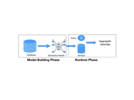
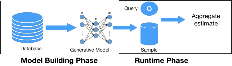
Our proposed approach proceeds in two phases. In the model building phase, we train a deep generative model $`M_{R}`$ over the dataset $`R`$ such that it learns the underlying data distribution. In this section, we assume that a single model is built for the entire dataset that we relax in Section 13. Once the DL model is trained, it can act as a succinct representation of the dataset. In the run-time phase, the AQP system uses the DL model to generate samples $`S`$ from the underlying distribution. The given query is rewritten to run on $`S`$. The existing AQP techniques could be transparently used to generate the aggregate estimate. 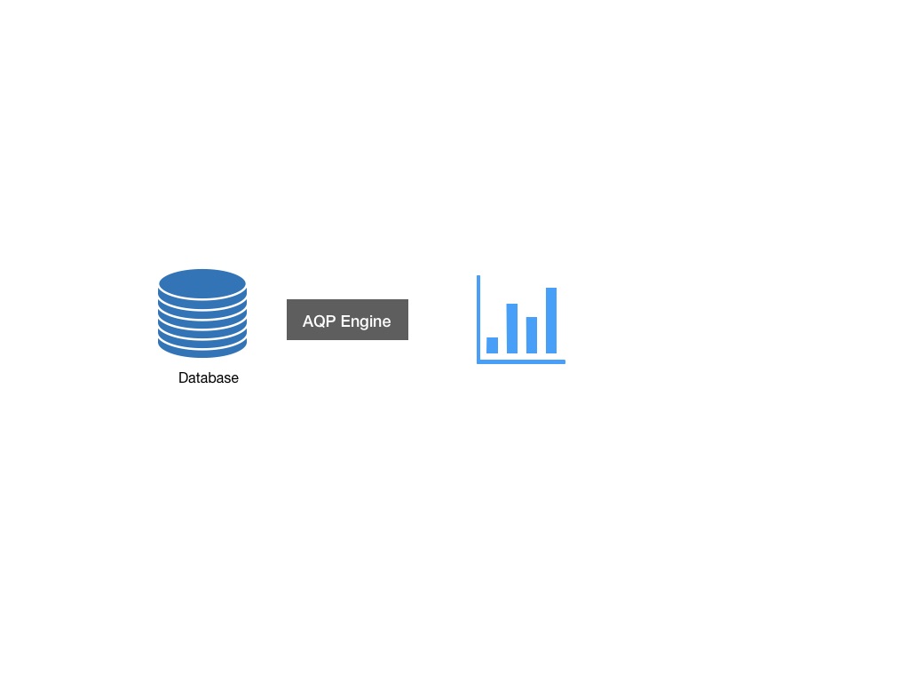Figure 1 illustrates our approach.

/>

Using VAE for AQP

In this subsection, we describe how to train a VAE over relational data and use it for AQP.

In contrast to homogeneous domains such as images and text, relations often consist of mixed data types that could be discrete or continuous. The first step is to represent each tuple $`t`$ as a vector of dimension $`d`$. For ease of exposition, we consider one-hot encoding and describe other effective encodings in Section 7.5. One-hot encoding represents each tuple as a $`d = \sum_{i=1}^{m} |Dom(A_i)|`$ dimensional vector where the position corresponding to a given domain value is set to 1. Each tuple in a relation $`R`$ with two binary attributes $`A_1`$ and $`A_2`$, is represented as a $`4`$ dimensional binary vector. A tuple with $`A_1=0,A_2=1`$ is represented as $`[1, 0, 0, 1]`$ while a tuple with $`A_1=1,A_2=1`$ is represented as $`[0, 1, 0, 1]`$. This approach is efficient for small attribute domains but becomes cumbersome if a relation has millions of distinct values.

Once all the tuples are encoded appropriately, we could use VAE to learn the underlying distribution. We denote the size of the input and latent dimension by $`d`$ and $`d'`$ respectively. For one hot encoding, $`d=\sum_{i=1}^{m} |Dom(A_i)|`$. As $`d'`$ increases, it results in more accurate learning of the distribution at the cost of a larger model. Once the model is trained, it could be used to generate samples $`X'`$. The randomly generated tuples often share similar statistical properties to tuples sampled from the underlying relation $`R`$ and hence are a viable substitute for $`R`$. One could apply the existing AQP mechanisms on the generated samples and use it to generate aggregate estimates along with confidence intervals.

The sample tuples are generated as follows: we generate samples from the latent space $`z`$ and then apply the decoder network to convert points in latent space to tuples. Recall from Section 6 that the latent space is often a probability distribution that is easy to sample such as Gaussian. It is possible to speed up the sampling from arbitrary Normal distributions using the reparameterization trick. Instead of sampling from a distribution $`N(\mu, \sigma)`$, we could sample from the standard Normal distribution $`N(0, 1)`$ with zero mean and unit variance. A sample $`\epsilon`$ from $`N(0, 1)`$ could be converted to a sample $`N(\mu, \sigma)`$ as $`z = \mu + \sigma \odot \epsilon`$. Intuitively, this shifts $`\epsilon`$ by the mean $`\mu`$ and scales it based on the variance $`\sigma`$.

Handling Approximation Errors.

We consider approximation error caused due to model bias and propose an effective rejection sampling to mitigate it.

Aggregates estimated over the sample could differ from the exact results computed over the entire dataset and their difference is called the sampling error. Both the traditional AQP and our proposed approach suffer from sampling error. The techniques used to mitigate it - such as increasing sample size - can also be applied to the samples from the generative model.

Another source of error is sampling bias. This could occur when the samples are not representative of the underlying dataset and do not approximate its data distribution appropriately. Aggregates generated over these samples are often biased and need to be corrected. This problem is present even in traditional AQP  and mitigated through techniques such as importance weighting  and bootstrapping .

Our proposed approach also suffers from sampling bias due to a subtle reason. Generative models learn the data distribution which is a very challenging problem - especially in high dimensions. A DL model learns an approximate distribution that is close enough. Uniform samples generated from the approximate distribution would be biased samples from the original distribution resulting in biased estimates. As we shall show later in the experiments, it is important to remove or reduce the impact of model bias to get accurate estimates. Bootstrapping is not applicable as it often works by resampling the sample data and performing inference on the sampling distribution from them. Due to the biased nature of samples, this approach provides incorrect results . It is challenging to estimate the importance weight of a sample generated by VAE. Popular approaches such as IWAE  and AIS  do not provide strong bounds for the estimates.

We advocate for a rejection sampling based approach  that has a number of appealing properties and is well suited for AQP. Intuitively, rejection sampling works as follows. Let $`x`$ be a sample generated from the VAE model with probabilities $`p(x)`$ and $`q(x)`$ from the original and approximate probability distributions respectively. We accept the sample $`x`$ with probability $`\frac{p(x)}{M \times q(x)}`$ where $`M`$ is a constant upper bound on the ratio $`p(x)/q(x)`$ for all $`x`$. We can see that the closer the ratio is to 1, the higher the likelihood that the sample is accepted. On the other hand, if the two distributions are far enough, then a larger fraction of samples will be rejected. One can generate arbitrary number of samples from the VAE model, apply rejection sampling on them and use the accepted samples to generate unbiased and accurate aggregate estimates.

In order to accept/reject a sample $`x`$, we need the value of $`p(x)`$. Estimating this value - such as by going to the underlying dataset - is very expensive and defeats the purpose of using generative models. A better approach is to approximately estimate it purely from the VAE model.

We leverage an approach for variational rejection sampling that was recently proposed in . For the sake of completeness, we describe the approach as applied to AQP. Please refer to  for further details. Sample generation from VAE takes place in two steps. First, we generate a sample $`z`$ in the latent space using the variational posterior $`q(z|x)`$ and then we use the decoder to convert $`z`$ into a sample $`x`$ in the original space. In order to generate samples from the true posterior $`p(z|x)`$, we need to accept/reject sample $`z`$ with acceptance probability

\begin{equation}
    a(z|x, M) = \frac{p(z|x)}{ M \times q(z|x)}
    \label{eq:acceptanceBasic}
\end{equation}

where $`M`$ is an upper bound on the ratio $`p(z|x) / q(z|x)`$. Estimating the true posterior $`p(z|x)`$ requires access to the dataset and is very expensive. However, we do know that the value of $`p(x, z)`$ from the VAE is within a constant normalization factor $`p(x)`$ as $`p(z|x) = \frac{p(x, z)}{p(x)}`$. Thus, we can redefine Equation [eq:acceptanceBasic] as

\begin{equation}
    a(z|x, M') = \frac{p(x, z)}{ M \times p(x) \times q(z|x)} = \frac{p(x, z)}{M' \times q(z|x)}
    \label{eq:acceptanceAdvanced}
\end{equation}

We can now conduct rejection sampling if we know the value of $`M'`$. First, we generate a sample $`z`$ from the variational posterior $`q(z|x)`$. Next, we draw a random number $`U`$ in the interval $`[0, 1]`$ uniformly at random. If this number is smaller than the acceptance probability $`a(z|x, M')`$, then we accept the sample and reject it otherwise. That way the number of times that we have to repeat this process until we accept a sample is itself a random variable with geometric distribution p = $`P(U \leq a(z|x,M'))`$; $`P(N=n)=(1-p)^{n-1}p, n \geq 1`$. Thus on average the number of trials required to generate a sample is $`E(N) = 1/p`$. By a direct calculation it is easy to show that $`p=1/M'`$. We set the value of $`M'`$ as $`M' = e^{-T}`$ where $`T \in [-\infty, +\infty]`$ is an arbitrary threshold function. This definition has a number of appealing properties. First, this function is differentiable and can be easily plugged into the VAE’s objective function thereby allowing us to learn a suitable value of $`T`$ for the dataset during training . 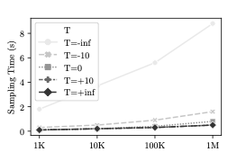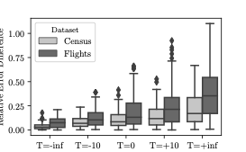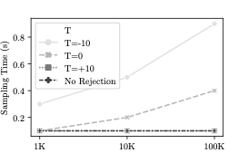Please refer to Section 16 for a heuristic method for setting appropriate values of $`T`$ during model building and sample generation. Second, the parameter $`T`$ when set, establishes a trade-off between computational efficiency and accuracy. If $`T \rightarrow +\infty`$, then every sample is accepted (no rejection) resulting into fast sample generation at the expense of the quality of the approximation to the true underlying distribution. In contrast when $`T \rightarrow -\infty`$, we ensure that almost every sample is guaranteed to be from the true posterior distribution, by making the acceptance probability small and as a result increasing sample generation time. Since $`a`$ should be a probability we change equation Equation [eq:acceptanceAdvanced] to:

\begin{equation}
    a(z|x, M') = \min \Big[ 1, \frac{p(x, z)}{M' \times q(z|x)} \Big]
    \label{eq:acceptanceFinal}
\end{equation}

Towards Accuracy Guarantees

Variational Autoencoder AQP Workflow

Algorithm [alg:VAEforAQP] provides the pseudocode for the overall workflow of performing AQP using VAE. In the model building phase, we encode the input relation $`R`$ using an appropriate mechanism (see Section 7.5). The VAE model is trained on the encoded input and stored along with appropriate metadata.

Making VAE practical for relational AQP

In this subsection, we propose two practical improvements for training VAE for AQP over relational data.

One-hot encoding of tuples is an effective approach for relatively small attribute domains. If the relation has millions of distinct values, then it causes two major issues. First, the encoded vector becomes very sparse resulting in poor performance . Second, it increases the number of parameters learned by the model thereby increasing the model size and the training time.

A promising approach to improve one-hot encoding is to make the representation denser using binary encoding. Without loss of generality, let the domain $`Dom(A_j)`$ be its zero-indexed position $`[0, 1, \ldots, |Dom(A_j)|-1]`$. We can now concisely represent these values using $`\lceil \log_2 |Dom(A_j)| \rceil`$ dimensional vector. Once again consider the example $`Dom(A_j) = \{Low, Medium, High\}`$. Instead of representing $`A_j`$ as a 3-dimensional vectors ($`001,010,100`$), we can now represent them in $`\lceil \log_2(3) \rceil = 2`$-dimensional vector $`\eta(Low)=00, \eta(Medium)=01, \eta(High)=10`$. This approach is then repeated for each attribute resulting a $`d = \sum_{i=1}^{n} \lceil \log_2 |Dom(A_i)| \rceil`$-dimensional vector (for $`n`$ attributes) that is exponentially smaller and denser than the one-hot encoding that requires $`\sum_{i=1}^{n} |Dom(A_i)|`$ dimensions.

Typically, samples are obtained from VAE in two steps: (a) generate a sample $`z`$ in the latent space $`z \sim q(z|x)`$ and (b) generate a sample $`x'`$ in the original space by passing $`z`$ to the decoder. While this approach is widely used in many domains such as images and music, it is not appropriate for databases. Typically, the output of the decoder is stochastic. In other words, for the same value of $`z`$, it is possible to generate multiple reconstructed tuples from the distribution $`p(x|z)`$. However, blindly generating a random tuple from the decoder output could return an invalid tuple. For images and music, obtaining incorrect values for a few pixels/notes is often imperceptible. However, getting an attribute wrong could result in a (slightly) incorrect estimate Typically, the samples generated are often more correct than wrong. We could minimize the likelihood of an aberration by generating multiple samples for the same value of $`z`$. In other words, for the same latent space sample $`z`$, we generate multiple samples $`X'=\{x'_1, x'_2, \ldots, \}`$ in the tuple space. These samples could then be aggregated to obtain a single sample tuple $`x'`$. The aggregation could be based on max (for each attribute $`A_j`$, pick the value that occurred most in $`X'`$) or weighted random sampling (for each attribute $`A_j`$, pick the value based on the frequency distribution of $`A_j`$ in $`X'`$). Both these approaches provide sample tuples that are much more robust resulting in better accuracy estimates.

Conclusion

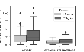
We proposed a model based approach for AQP and demonstrated experimentally that the generated samples are realistic and produce accurate aggregate estimates. We identify the issue of model bias and propose a rejection sampling based approach to mitigate it. We proposed dynamic programming based algorithms for identifying optimal partitions to train multiple generative models. Our approach could integrated easily into AQP systems and can satisfy arbitrary accuracy requirements by generating as many samples as needed without going back to the data. There are a number of interesting questions to consider in the future. Some of them include better mechanisms for generating conditional samples that satisfy certain constraints. Moreover, it would be interesting to study the applicability of generative models in other data management problems such as synthetic data generation for structured and graph databases extending ideas in .