Customer temporal behavioral data was represented as images in order to perform churn prediction by leveraging deep learning architectures prominent in image classification. Supervised learning was performed on labeled data of over 6 million customers using deep convolutional neural networks, which achieved an AUC of 0.743 on the test dataset using no more than 12 temporal features for each customer. Unsupervised learning was conducted using autoencoders to better understand the reasons for customer churn. Images that maximally activate the hidden units of an autoencoder trained with churned customers reveal ample opportunities for action to be taken to prevent churn among strong data, no voice users.
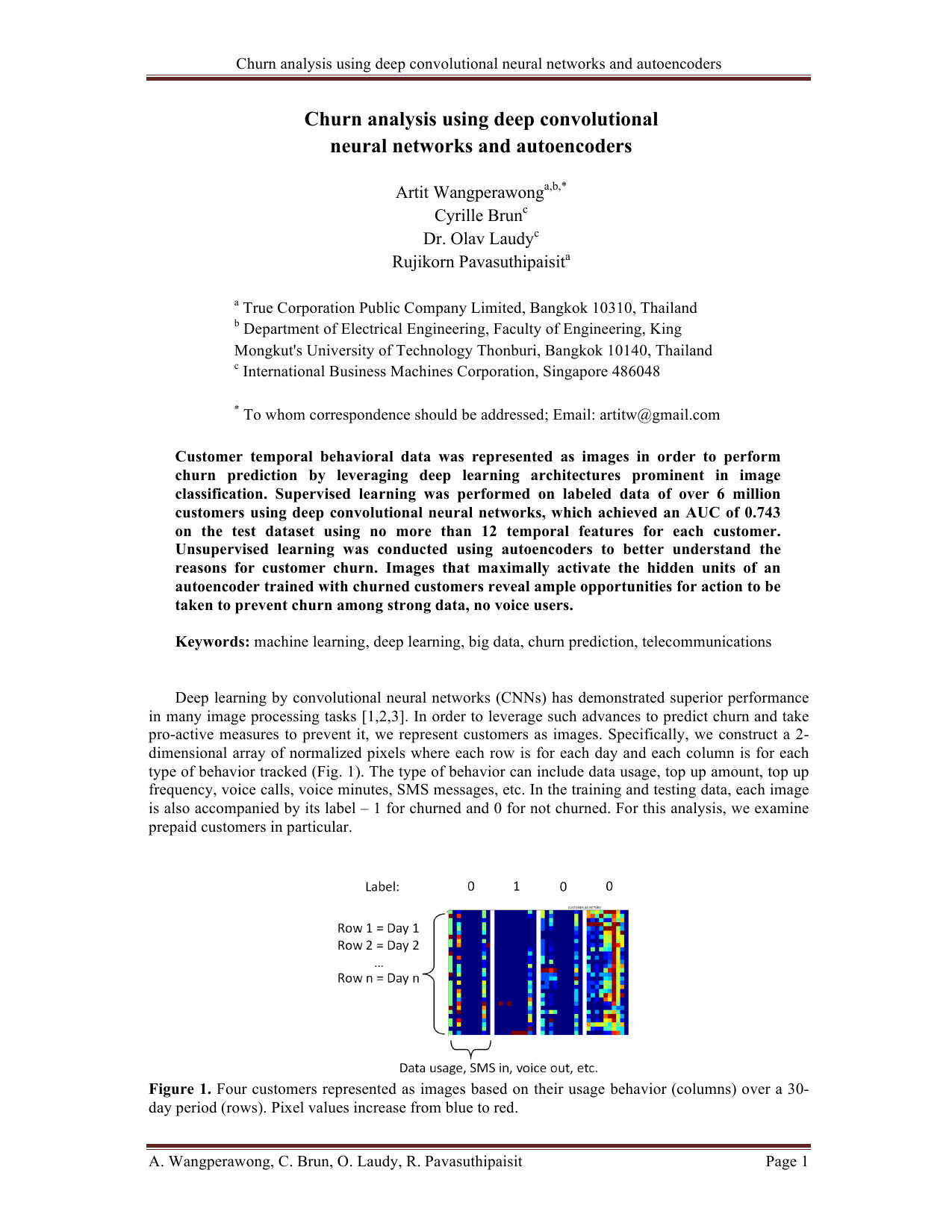
Deep learning by convolutional neural networks (CNNs) has demonstrated superior performance in many image processing tasks [1,2,3]. In order to leverage such advances to predict churn and take pro-active measures to prevent it, we represent customers as images. Specifically, we construct a 2dimensional array of normalized pixels where each row is for each day and each column is for each type of behavior tracked (Fig. 1). The type of behavior can include data usage, top up amount, top up frequency, voice calls, voice minutes, SMS messages, etc. In the training and testing data, each image is also accompanied by its label -1 for churned and 0 for not churned. For this analysis, we examine prepaid customers in particular. In order to determine the labels and the specific dates for the image, we first define churn, last call and the predictor window according to each customer's lifetime-line (LTL). This is best understood by viewing Fig. 2 from right to left. The first item is the churn assessment window, which we have chosen to be 30 days. If the customer registers any activity within these 30 days, we label them with 0 for active/not-churned. In Fig. 2, a green circle demarks this label for the first, top-most customer LTL. If the customer has no activity in this time frame, then we label them as 1 for churned. These are the second and third LTLs in Fig. 2. Next, we define the last call, which is the latest call occurring in the 14-day last call window of Fig. 2. If there is no call within this window, we exclude the customer from our analysis because we consider the customer to have churned long before we are able to take pro-active retention measures. We then look 14 days back from the last call to define the end of the predictor window. We used a 30day predictor window for our analyses here, but it is conceivable to vary this time frame to yield improved results. Note that the exact dates of the predictor window depend on each customer's usage behavior because we want to use the same protocol to prepare new, unlabeled data for the actual prediction. After creating the training and testing images for each customer according to the customer LTL method explained above, we feed them through deep CNNs similar to those used successfully for image classification. One such architecture is shown in Fig. 3, which we call DL-1. This architecture consists of two consecutive convolutional layers, followed by a 2x1 max pooling layer, a fullyconnected layer of 128 units, and a softmax output of two units for the binary classification. The first convolutional layer involves four filters of size 7x1, which pans across each usage behavior column over a period of seven days. We chose seven days to analyze the customers' weekly patterns across each usage behavior type at a time. Each filter maintains its shared weights and biases throughout the convolution as commonly employed in image processing. The outputs are then convoluted further in the second convolutional layer, where two filters of size 1x10 pan across all usage behavior features and one row of output from the first convolutional layer. This filter is intended to analyze the customers' usage across all variables at a given time.
After the convolutions, a max pooling layer of size 2x1 is applied that is intended to assist with translational invariance [4]. Next, the fully-connected layer flattens and prepares the data for the softmax output binary classifier. Training and testing this architecture end-to-end yields results superior to that of a CHAID decision tree model when judging by the area-under-the-curve (AUC) benchmark (Table 1). The AUC of a receiver operating curve is a commonly accepted benchmark for comparing models; it accounts for both true and false positives [5,6]. Note that DL-1 was trained for 20 epochs using a binary cross-entropy loss function [7], rectified linear unit activation functions, and stochastic gradient descent by backpropagation [8] in batch sizes of 1000 with adaptive learning rates [9]. Comparing the SPSS CHAID model and the DL-1 model, we see that although both cases exhibit overfitting, the deep learning implementation is superior in both training and testing.
We tested various deep learning hyperparameters and architectures and found the best results in DL-2. DL-2 includes two more features, topup count/amount, and comprises of a 12x7x1 convolutional layer with 0.25 dropout [10], followed by a 2x1 max pooling layer, a 7x1x12 convolutional layer, a 2x1 max pooling layer, a fully-connected layer of 100 units with 0.2 dropout, a fully-connected layer of 40 units with 0.2 dropout, a fully-connected layer of 20 units with 0.2 dropout, and a softmax output of two units for the binary classification. The use of more fully connected layers and dropout in DL-2 appears to reduce overfitting, as evident in the DL-2 AUCs for training and testing datasets in Table 1. While the training AUC is less than that of DL-1, the test AUC is significa
This content is AI-processed based on open access ArXiv data.