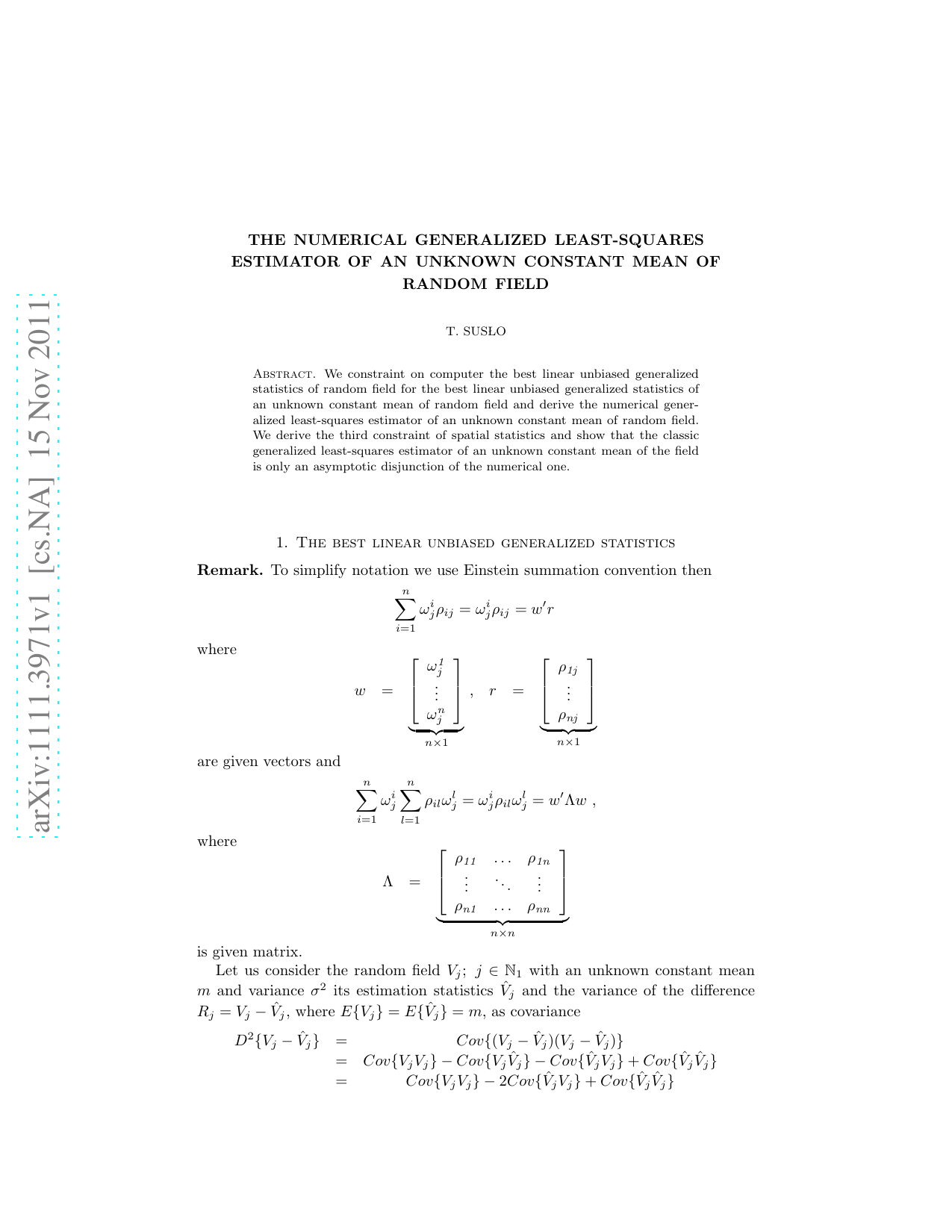
We constraint on computer the best linear unbiased generalized statistics of random field for the best linear unbiased generalized statistics of an unknown constant mean of random field and derive the numerical generalized least-squares estimator of an unknown constant mean of random field. We derive the third constraint of spatial statistics and show that the classic generalized least-squares estimator of an unknown constant mean of the field is only an asymptotic disjunction of the numerical one.
Remark. To simplify notation we use Einstein summation convention then Let us consider the random field V j ; j ∈ N 1 with an unknown constant mean m and variance σ 2 its estimation statistics Vj and the variance of the difference R j = V j -Vj , where E{V j } = E{ Vj } = m, as covariance
and the linear estimation statistics (weighted variable) Vj = n i=1 ω i j V i = ω i j V i ; j ⊂ i = 1, . . . , n at j ≥ n + 1 then
where ρ ij ; i = 1, . . . , n is given vector of correlations and ρ il ; i, l = 1, . . . , n is given (symmetric) matrix of correlations (see Appendix A). The unbiasedness constraint (the first constraint on the estimation statistics)
gives the first equation
The minimization constraint (the second constraint on the estimation statisticsthe statistics is the best)
produces n equations in n + 1 unknowns the kriging weights ω i j and a Lagrange parameter µ
this system of equations if multiplied by ω i j
and substituted into
since variance of the (estimation) statistics is minimized
.
Remark. When we consider an independent set of the random variables V i ; i = 1, . . . , n with an unknown constant mean m and variance σ 2 the best linear unbiased ordinary (estimation) statistics Vj = ω i j V i of the field V j ; j ⊂ i = 1, . . . , n has the asymptotic property
0 whilst for spatial dependence between random variables (the best linear unbiased generalized statistics) we get (see Appendix B)
Due to different asymptotic limits between (7) and (8) the ordinary least-squares estimator of an unknown constant mean m of the field, the best linear unbiased estimator of an unknown constant mean m of the field, can not be so easy generalized (like it was in past).
Let us constraint the best linear unbiased generalized (estimation) statistics Vj = ω i j V i of the random field V j ; j ⊂ i = 1, . . . , n, when for finite n and j → ∞ the vector of correlations simplifies to
for the co-ordinate independent statistics of an unknown constant mean of the field V j with the constraint on (11)
given by constrained from (11) (13) µ 1 j = -ξ and from (9) the system of equations ( 6)
where
with the solution
of the classic best linear unbiased generalized statistics for finite n and j → ∞ of an unknown constant mean of the field (16) lim
with constrained minimized variance of the best linear unbiased generalized (estimation) statistics (4) as its variance (from(10) and ( 13))
with the classic generalized least-squares estimator for finite n and j → ∞ of an unknown constant mean m of the field
To remove the asymptotic limit of the classic best linear unbiased generalized statistics for finite n and j → ∞ of an unknown constant mean m = E{V j } of the field V j with the constraint (12)
the best linear unbiased generalized (estimation) statistic of the field V j ; j ⊂ i = 1, . . . , n at finite j ≥ n
given by the kriging algorithm (6) for n = 182
the negative correlation function with the parameter t = 182 + 1, . . . , 182 + 139 was constrained (from (5)) on computer (139 times) for the numerical best linear unbiased generalized statistics for finite n at finite j of an unknown constant mean m = E{V j } of the field V j with the third constraint of spatial statistics
with constrained minimized variance of the best linear unbiased generalized (estimation) statistics (4) as its variance (see Fig. 1).
Our aim was to derive for the negative correlation function ( 18) with the parameter t = 182 + 1, . . . , 182 + 139 the numerical generalized least-squares estimator ω i j v i of an unknown constant mean m = E{V j } of the field V j in fact the proper best linear unbiased (generalized) estimator of an unknown constant mean m = E{V j } of the field V j given at finite j ≥ n + 1 = 182 + 1 by numerical approximation to root of the equation (20). This (co-ordinate dependent) generalized least-squares estimator ω i j v i was compared to the (co-ordinate independent) classic generalized least-squares estimator lim j→∞ ω i j v i of an unknown constant mean of the field (17)
based on the same observation an initial amplification v i = v 1 , . . . , v 182 of long-lived asymmetric index profile recorded by 600 close quotes of Xetra Dax Index shown Long-lived asymmetric index profile,Xetra Dax Index from 23 X 1997 up to 10 III 2000 (600 close quotes) the numerical generalized least-squares estimator ω i j v i of an unknown constant mean m = E{V j } of the field V j ; j ⊂ i = 1, . . . , 182 (black dots) based on v i = v 1 , . . . , v 182 is compared for the negative correlation function (18) with the parameter t = 182+1, . . . , 182+139 at finite j ≥ n+1 = 182+1 to the classic generalized least-squares estimator lim j→∞ ω i j v i of an unknown constant mean m = E{V j } of the field V j (grey line) with the same correlation function and based on the same sample. The classic estimator is the first approximation of the numerical estimator at final j = 577 for final t = 182 + 139. The dashed vertical line represents j =
This content is AI-processed based on open access ArXiv data.

