New Electrodynamics of Pulsars

arXiv:1111.3377v1 [astro-ph.HE] 14 Nov 2011 New Electrodynamics of Pulsars Andrei Gruzinov CCPP, Physics Department, New York University, 4 Washington Place, New York, NY 10003 ABSTRACT We have recently proposed that Force-Free Electrodynamics (FFE) does not apply to pulsars – pulsars should be described by the high-conductivity limit of Strong-Field Electrodynamics (SFE), which predicts an order-unity damping of the Poynting flux, while FFE postulates zero damping. The strong damping result has not been accepted by several pulsar experts, who claim that FFE basically works and the Poynting flux damping can be arbitrarily small. Here we consider a thought experiment – cylindrical periodic pulsar. We show that FFE is incapable of describing this object, while SFE predictions are physically plausible. The intrinsic breakdown of FFE should mean that the FFE description of the singular current layer (the only region of magnetosphere where FFE and the high-conductivity SFE differ) is incorrect. Then the high-conductivity SFE should be the right theory for real pulsars too, and the pure-FFE description of pulsars should be discarded. 1. Introduction We have shown that ideal pulsars calculated in the high-conductivity limit of Strong-Field Elec- trodynamics (SFE 1) dissipate an order-unity frac- tion of the Poynting flux in the singular current layer (SL), which in SFE exists only outside the light cylinder (Gruzinov 2011ab). This result, if true, is obviously important for interpreting pul- sar phenomenology. SL should be the most pow- erful site of pulsar emission (cf Bai & Spitkovsky 2010). Two groups of prominent pulsar experts dis- agree with the strong-damping result (Li et al 2011, Kalapotharakos et al 2011) and claim that FFE (as it applies to pulsars) works exactly as it has always been thought to work, so that the SL damping can be arbitrarily small. Here we calculate FFE and SFE magneto- spheres of an artificial system – cylindrical pe- riodic pulsar. We consider an ideally conducting cylinder rotating around its axis. The cylinder is magnetized axisymmetrically and periodically along the axis. 1Maxwell plus j = σE in the right frame (Gruzinov 2011a). 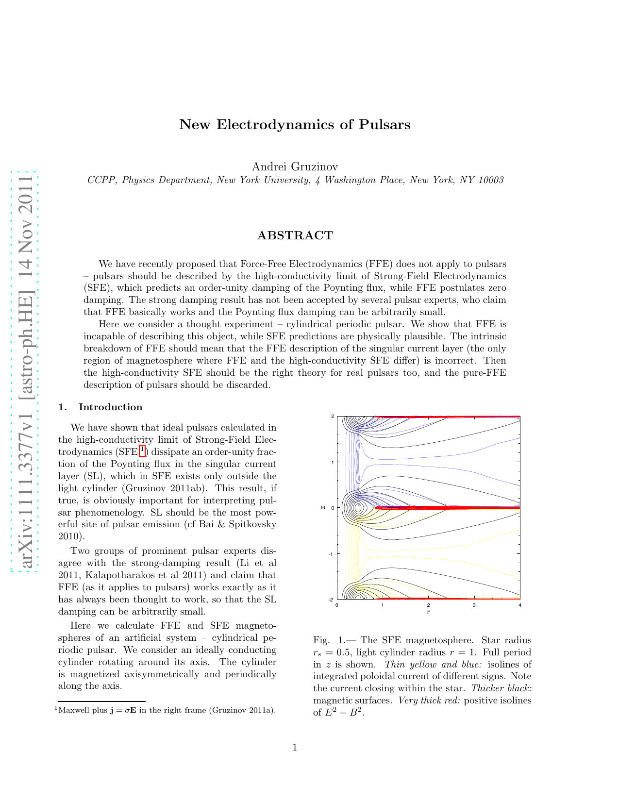0 1 2 3 4 -2 -1 0 1 2 Fig. 1.— The SFE magnetosphere. Star radius rs = 0.5, light cylinder radius r = 1. Full period in z is shown. Thin yellow and blue: isolines of integrated poloidal current of different signs. Note the current closing within the star. Thicker black: magnetic surfaces. Very thick red: positive isolines of E2 −B2. 1 It is clear without any calculations that the FFE magnetosphere of the cylindrical periodic pulsar is unphysical. We calculate the FFE mag- netosphere anyway (§2), not only as a counter for the SFE magnetosphere (§3), but also to stress that FFE predictions are ambiguous and incor- rect. The SFE magnetosphere, on the other hand, does look reasonable (Fig.1). The order of magnitude of the SL damping must be decided by the microphysics rather than by the global geometry of the problem. We there- fore propose that SFE is in the right also when applied to real pulsars. 2. FFE magnetosphere The FFE magnetosphere is calculated by the standard CKF procedure (Contopoulos, Kazanas & Fendt 1999): (1 −r2)∆ψ −2 r ∂rψ + F(ψ) = 0, (1) ψ(rs, z) = f(z), (2) ψ(r > 1, 0) = ψ(1, 0), (3) ψ(r, H) = 0. (4) Here r is the cylindrical radius, the light cylinder is at r = 1, rs is the radius of the cylindrical star, H is the quarter-period, ψ is the magnetic stream function and electric potential, F ≡A(dA/dψ), A is twice the integrated poloidal current. The function f(z) represents the surface mag- netization of the star. For no particular reason, we set rs = 0.5, H = 1, and f(z) ∝ X k (−1)ke−20(z−2k)2. (5) This gives well-isolated periodically repeating re- gions of alternating sign ψ. If the star were not rotating, each region of sign-definite ψ would have field lines closing onto itself. In truth, there is one ill-defined reason for choosing to have well-isolated regions of sign- definite ψ. One would think that these regions work roughly as separate pulsars, and the CKF procedure must be applicable to each of the “pul- sars” in a more or less unmodified form. Then FFE is expected to make unambiguous predictions regarding the cylindrical pulsar and its SL. 0 0.5 1 1.5 0 0.5 1 1.5 Fig. 2.— The “standard” FFE magnetosphere. Thick magenta: boundary of the star and the quarter-period. Thin black: magnetic surfaces. The poloidal current closes within each half-period of sign-definite ψ by flowing in the equatorial plane from infinity to the light cylinder and then flow- ing to the star in the magnetic separatrix (the last closed magnetic surface). 0 0.5 1 1.5 0 0.5 1 1.5 Fig. 3.— A possible FFE magnetosphere. There is no singular poloidal current in the equatorial planes and in the magnetic separatrices. The cur- rent closes within the star. 2 We first solve the problem (1) just as described by CKF, and get the quarter-period shown in Fig.2. Next we note that for our

This content is AI-processed based on open access ArXiv data.