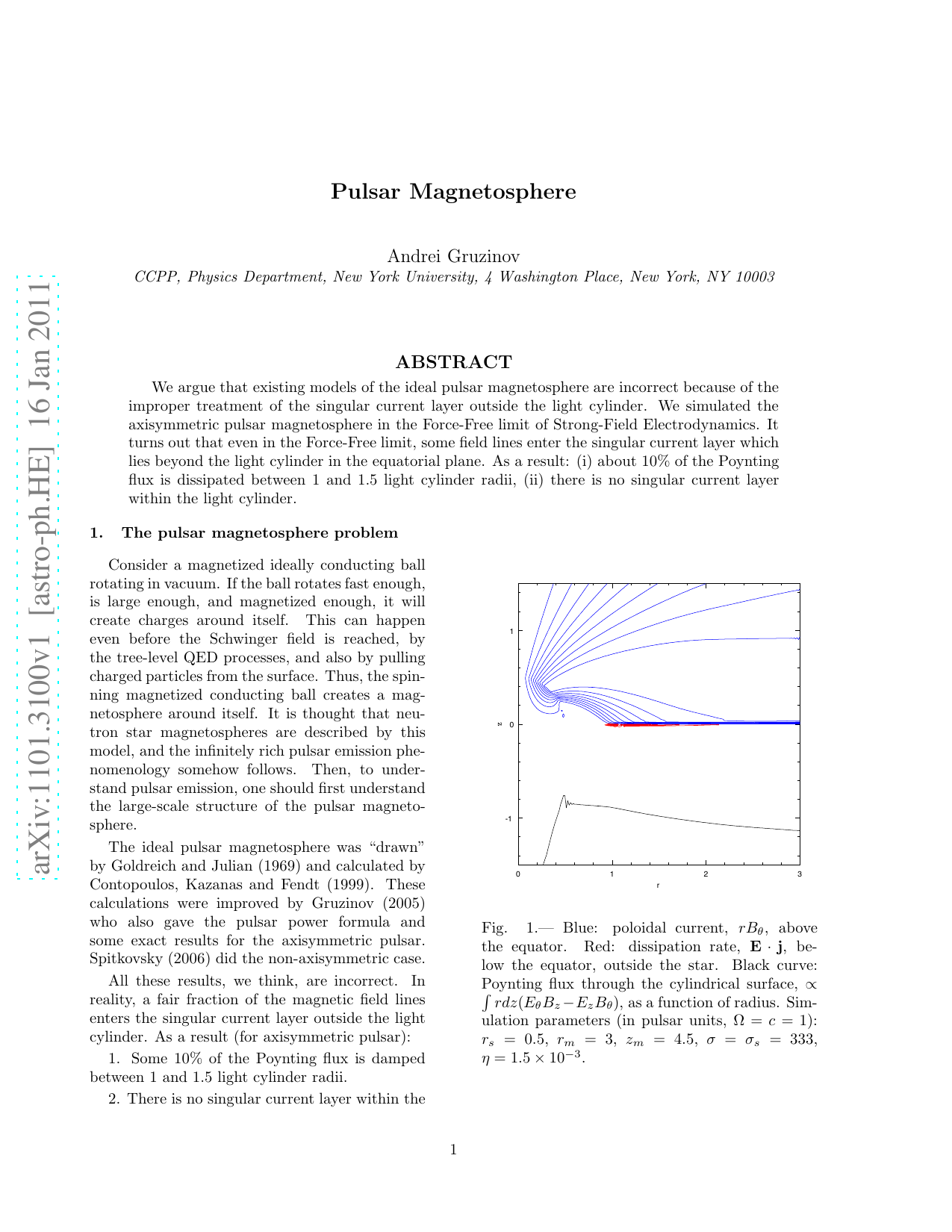
We argue that existing models of the ideal pulsar magnetosphere are incorrect because of the improper treatment of the singular current layer outside the light cylinder. We simulated the axisymmetric pulsar magnetosphere in the Force-Free limit of Strong-Field Electrodynamics. It turns out that even in the Force-Free limit, some field lines enter the singular current layer which lies beyond the light cylinder in the equatorial plane. As a result: (i) about 10% of the Poynting flux is dissipated between 1 and 1.5 light cylinder radii, (ii) there is no singular current layer within the light cylinder.
Consider a magnetized ideally conducting ball rotating in vacuum. If the ball rotates fast enough, is large enough, and magnetized enough, it will create charges around itself. This can happen even before the Schwinger field is reached, by the tree-level QED processes, and also by pulling charged particles from the surface. Thus, the spinning magnetized conducting ball creates a magnetosphere around itself. It is thought that neutron star magnetospheres are described by this model, and the infinitely rich pulsar emission phenomenology somehow follows. Then, to understand pulsar emission, one should first understand the large-scale structure of the pulsar magnetosphere.
The ideal pulsar magnetosphere was “drawn” by Goldreich and Julian (1969) and calculated by Contopoulos, Kazanas and Fendt (1999). These calculations were improved by Gruzinov (2005) who also gave the pulsar power formula and some exact results for the axisymmetric pulsar. Spitkovsky (2006) did the non-axisymmetric case.
All these results, we think, are incorrect. In reality, a fair fraction of the magnetic field lines enters the singular current layer outside the light cylinder. As a result (for axisymmetric pulsar):
Some 10% of the Poynting flux is damped between 1 and 1.5 light cylinder radii.
There is no singular current layer within the
The error of all existing calculations comes from the improper treatment of the singular current layer outside the light cylinder. Here we describe simulations of the pulsar magnetosphere which resolve all singularities -we don’t use any boundary conditions, not even at the surface of the star.
Our numerical simulations are done in the FFE (Force-Free Electrodynamics) limit of the SFE (Strong-Field Electrodynamics). We describe FFE and SFE in the next section. In §3, we describe the simulations.
Both FFE and SFE are plasma physics models which describe the plasma implicitly (Gruzinov 2008). Namely, one solves the Maxwell equations
or in the 3+1 split,
supplemented by some Ohm’s law, which gives j in terms of the electromagnetic field only.
In FFE, the Ohm’s law is
Here the scalar E 0 is the proper electric field, defined by
The physical meaning of the FFE Ohm’s law is as follows. For any electromagnetic field, at any event, there is a one-parameter family of good frames, where E is parallel to B. FFE postulates, that in any good frame, the electric field vanishes and the current flows along the magnetic field.
In SFE, the Ohm’s law is
Here F is the dual tensor, and σ is the conductivity scalar.
The physical meaning of the SFE Ohm’s law is as follows. At each event, the family of good frames contains the best frame, where the charge density vanishes, and the current σE 0 flows along common direction of the electric and magnetic fields. If E 0 = 0, the charge density ρ has to move at the speed of light, so that j µ j µ = 0.
In numerical simulations, one uses the 3+1 split, and the FFE Ohm’s law becomes
(6) The SFE Ohm’s law is
where
In the limit of high conductivity, SFE reduces to FFE (Gruzinov 2008). This might seem strange, because SFE postulates that the 4-current is always space-like or null-like, j µ j µ ≤ 0, while FFE admits time-like currents, j µ j µ ≡ ρ 2j 2 > 0. But it turns out, that SFE handles the time-like currents by constantly switching the direction of the null-like current, such that the time-averaged current becomes time-like.
FFE can be applied only to initial electromagnetic fields of special geometry -with the electric field everywhere smaller than and perpendicular to the magnetic field. SFE applies to arbitrary initial field.
FFE is ideal, the electromagnetic energy is conserved. SFE is semi-ideal, the electromagnetic energy is non-increasing, but it remains exactly constant for all fields with E 0 = 0.
In cylindrical coordinates (r, θ, z), assuming axisymmetric field, we numerically integrate the following equations
The small diffusivity η is added for regularization.
The equations are solved in a volume
The boundary conditions at r m are
The boundary conditions at z m are
The initial conditions are
The Ohm’s law outside the star
is given by eq.( 7), with the field invariants regularization of (Gruzinov 2008). The Ohm’s law inside the star is the standard relativistic Ohm’s law in a moving medium
Here σ s is the conductivity of the star; v is the uniform rotation, and j e is the external currentboth purely toroidal, inside the star:
γ s is the Lorentz factor of v.
The numerical scheme was just the direct primitive discretization of the PDEs. The only subtlety is the time step. Since SFE handles the time-like current regions by permanently switching the sign of B 0 , one needs to reduce the time step (after saturation of the fields) to get accurate final results.
We increased the spatial resolution and conductivities σ and σ s , and decreased the diffusivity η, until the final magnetosphere outside the star showed clear signs of saturation. The
This content is AI-processed based on open access ArXiv data.