Nesterov's accelerated gradient methods (AGM) have been successfully applied in many machine learning areas. However, their empirical performance on training max-margin models has been inferior to existing specialized solvers. In this paper, we first extend AGM to strongly convex and composite objective functions with Bregman style prox-functions. Our unifying framework covers both the $\infty$-memory and 1-memory styles of AGM, tunes the Lipschiz constant adaptively, and bounds the duality gap. Then we demonstrate various ways to apply this framework of methods to a wide range of machine learning problems. Emphasis will be given on their rate of convergence and how to efficiently compute the gradient and optimize the models. The experimental results show that with our extensions AGM outperforms state-of-the-art solvers on max-margin models.
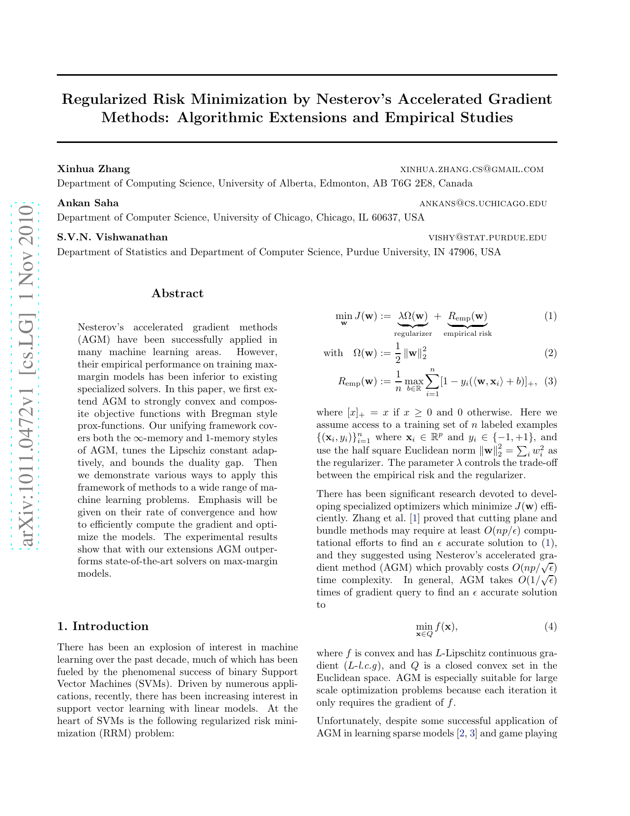
There has been an explosion of interest in machine learning over the past decade, much of which has been fueled by the phenomenal success of binary Support Vector Machines (SVMs). Driven by numerous applications, recently, there has been increasing interest in support vector learning with linear models. At the heart of SVMs is the following regularized risk minimization (RRM) problem: min w J(w) := λΩ(w) regularizer + R emp (w) empirical risk (1) with Ω(w) := 1 2 w 2 2
(2)
where [x] + = x if x ≥ 0 and 0 otherwise. Here we assume access to a training set of n labeled examples {(x i , y i )} n i=1 where x i ∈ R p and y i ∈ {-1, +1}, and use the half square Euclidean norm w 2 2 = i w 2 i as the regularizer. The parameter λ controls the trade-off between the empirical risk and the regularizer.
There has been significant research devoted to developing specialized optimizers which minimize J(w) efficiently. Zhang et al. [1] proved that cutting plane and bundle methods may require at least O(np/ǫ) computational efforts to find an ǫ accurate solution to (1), and they suggested using Nesterov’s accelerated gradient method (AGM) which provably costs O(np/ √ ǫ) time complexity. In general, AGM takes O(1/ √ ǫ) times of gradient query to find an ǫ accurate solution to
where f is convex and has L-Lipschitz continuous gradient (L-l.c.g), and Q is a closed convex set in the Euclidean space. AGM is especially suitable for large scale optimization problems because each iteration it only requires the gradient of f .
Unfortunately, despite some successful application of AGM in learning sparse models [2,3] and game playing [4], it does not compare favorably to existing specialized optimizers when applied to training large margin models [5]. It turns out that special structures exist in those problems, and to make full use of AGM, one must utilize the computational and statistical properties of the learning problem by properly reformulating the objectives and tailoring the optimizers accordingly.
To this end, our first contribution is to show that in both theory and practice smoothing R emp (w) as in [6] is advantageous to the primal-dual versions of AGM. The dual of ( 1) is
Comparing ( 4) with ( 1) and ( 5), it seems more natural to apply AGM to (5) because it is smooth. However in practice, most α i at the optimum will be on the boundary of [0, n -1 ]. According to [7], such α i ’s are easy to identify and so the corresponding entries in the gradient are wasted by AGM. This structure of support vector is unique for max-margin models, which will also be manifested in our experiments (Section 6).
In contrast, smoothing R emp has a lot of advantages. First, it directly optimizes in the primal J, avoiding the indirect translation from the dual solution to the primal. Second, the resulting optimization problem is unconstrained. If Ω is strongly convex, then linear convergence can be achieved. Third, gradient of the smoothed Remp can often be computed efficiently, and details will be given in Section 5.4. Fourth, the diameter of the dual space Q 2 often grows slowly with n, or even decreases. This allows using a loose smoothing parameter. Fifth, in practice most α i at the optimum are 0, where Remp best approximates R emp . Therefore, the approximation is actually much tighter than the worst case theoretical bound, and a good solution for Remp is more likely to optimize R emp too. Last but most important, the smoothed Remp themselves are reasonable risk measures [8], which also deliver good generalization performance in statistics. Now that it is much easier to optimize the smoothed objectives, a model which generalizes well can be quickly obtained with the homotopy scheme (i.e. anneal the smoothing parameter).
Using the same idea of smoothing R emp , AGM can be applied to a much wider variety of RRM problems by utilizing its composite structure. Given a model ψ of R, if Ω(w) + ψ(w) can be solved efficiently, then [9] showed that Ω(w) + R(w) can be solved in O(1/ √ ǫ) steps, even if Ω is not differentiable, e.g. L 1 norm [10].
Similar approach is applied to the L 1,∞ regularizer and the elastic net [11] regularizer by [12]:
This Ω is strongly convex with respect to (wrt) the L 2 norm, and similarly in many RRM problems Ω is strongly convex wrt some norm • . For example, the relative entropy regularizer in boosting [13]:
is strongly convex wrt L 1 norm, and the log determinant of a matrix in [14][15][16]:
is strongly convex wrt the Frobenius norm. By exploiting the strong convexity, [17] accelerated the convergence rate from O(1/ √ ǫ) to O(log 1 ǫ ). However, the prox-function in this case must be strongly convex wrt • too. Existing methods either ignore the strong convexity in Ω [9], or restrict the norm to L 2 [10,17]. As one major contribution of this paper, we extend AGM to exploit this strong convexity in the context of Bregman divergence. In particular, we allow Ω to be strongly convex wrt a Bregman divergence indu
This content is AI-processed based on open access ArXiv data.

