GPU has a significantly higher performance in single-precision computing than that of double precision. Hence, it is important to take a maximal advantage of the single precision in the CG inverter, using the mixed precision method. We have implemented mixed precision algorithm to our multi GPU conjugate gradient solver. The single precision calculation use half of the memory that is used by the double precision calculation, which allows twice faster data transfer in memory I/O. In addition, the speed of floating point calculations is 8 times faster in single precision than in double precision. The overall performance of our CUDA code for CG is 145 giga flops per GPU (GTX480), which does not include the infiniband network communication. If we include the infiniband communication, the overall performance is 36 giga flops per GPU (GTX480).
CPU has been improving its computing performance but does not yet quench the thirst of those demanding users who need more computing power for their numerical challenges such as lattice QCD. Graphic processing units (GPU) opens a new era for high performance computing. GPU is originally designed to handle 3-dimensional graphic images. To achieve extremely high performance with geometric data, GPU is designed of simple and tiny processors. More modules are used for the data processing and, not for the data cache, nor for the flow control. Hence, GPU are very different from typical CPUs by construction. GPUs are very appropriate for highly intensive and parallelized scientific computation. At the beginning, programming GPU was quite challenging and difficult. Recently, Nvidia has introduced the CUDA library, which allow the users to program the code for GPU easily.
Since then, there have been several ways to program the GPU code: the Nvidia CUDA, Open Graphic Library (Open GL), and Open Computing Language (Open CL) APIs. In this paper, we focus on CUDA and its applications. The CUDA provides us a user-friendly programming environment based on the C, C++ programming language for GPU. All of our CPS library codes are compiled and tested in CUDA version 3.2 and compute capability 1.3 mode. We made the CUDA version of CG subroutines that were implemented as a part of the Columbia Physics System (CPS) library.
Conjugate gradient (CG) algorithm [7] is an iterative method for solving a linear algebraic equation of the following form. b = Ax ,
where A is a n × n positive definite Hermitian matrix. x and b are complex vectors in the n dimensional space. Matrix A and vector b are given and x is a solution vector that we want to obtain.
Using the CG method we can get the solution x up to the numerical precision what we want to achieve.
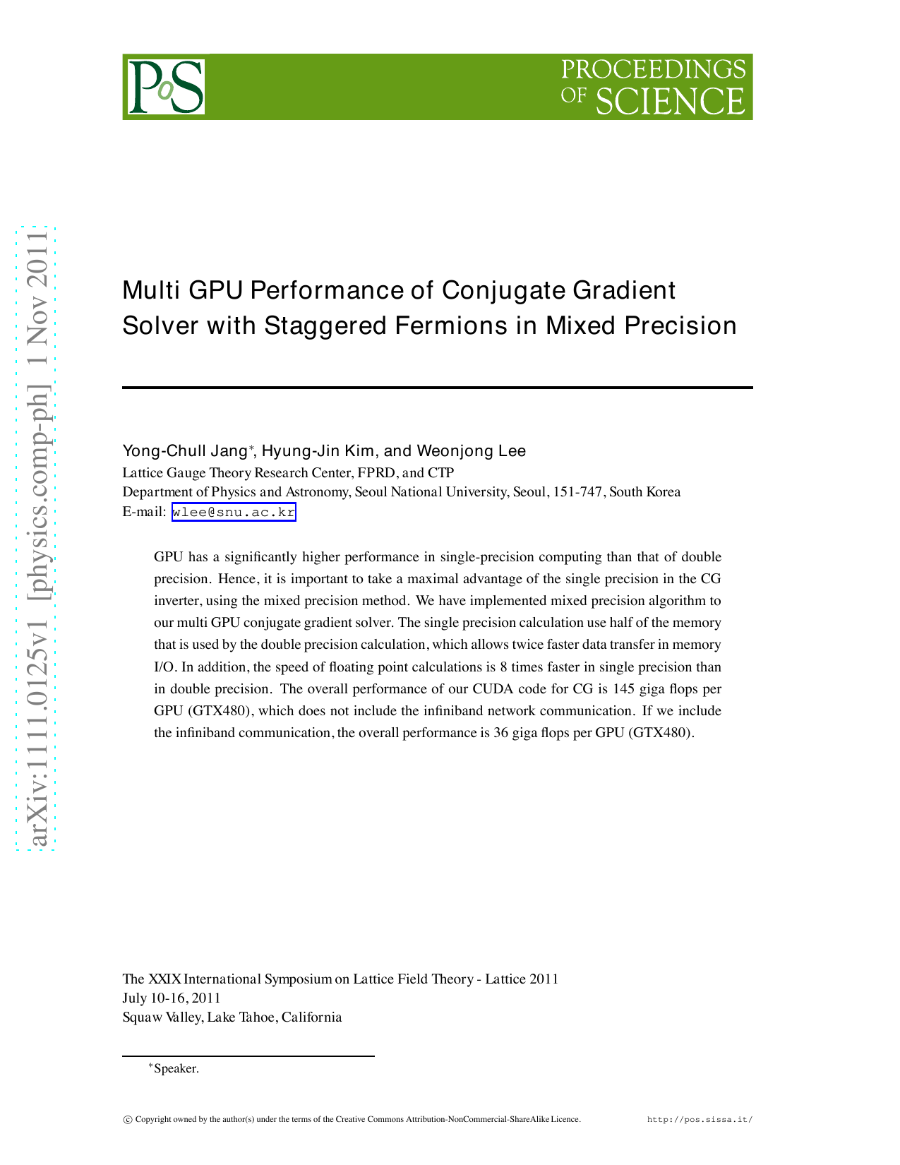
In Fig. 1, we show the structure of CG algorithm. In the CG sequence, we have a number of linear algebra equations such as vector addition, dot product, and scalar multiplication and so on. All of these linear algebra operations are implemented using CUDA library. Because most of these operations are not dominant part in CG operation, there is no special applied optimization for those functions except Dirac operation.
In Fig. 1, Ad and Ax are Dirac operations with staggered fermions [8]. Basically, the Dirac operation is a matrix-vector multiplication. This is the most dominant part in CG sequence. The matrix A is defined as follows. h = Aχ (2.2)
Here, the phase factor η µ (x) is multiplied in advance to the gauge link U µ at the gauge link preconditioning part of CPS library. h is a given as a source vector and χ is a staggered fermion field which corresponds to the CG solution.
At one site of the lattice, a single Dirac operation Dχ(x) needs 1584 bytes of data transfer and 576 number of floating point calculations. Let us consider a MILC fine lattice of 28 3 × 96. A single Dirac operation Dχ(x) over the entire, even sites of the lattice needs 0.6 billion number of floating point calculations. And it also needs 1.6 giga bytes of data transfer. As a result, when we use GPUs for CG operations, it is easy to find out that the bottle neck is on the data transfer rather then numerical operation.
Historically, there exists a significant gap between single precision performance and double precision performance in GPUs. In the case of the Nvidia GTX480 GPU, the single precision calculation runs 8 times faster than the double precision calculation.
How much we can accelerate the program is depend on the ratio of arithmetic operations and data I/O1 . The data I/O access is dominant in CG. It is the main bottle-neck in CG algorithm. Here, we do not include the infiniband network communication in the data I/O. So, by using the single precision data, the main benefit from it is that we can reduce the data traffic by a factor of 2, between GPU processor and GPU device memory.
To improve this performance of the CG program, the mixed precision method has been used. Mixed precision is implemented by iterative refinement algorithm [2]. The main idea of the iterative refinement is using two types of iterative loops to get the true solution value. At first, by using the single precision iteration, we can approach fast to the roughly estimated solution within inner loop tolerance. And next, double precision or more precise iteration can be used to get the more accurate solution within the outer loop error range. The iterative refinement procedure in CG is illustrated in Fig. 2. In the inner loop, Ay = r k is solved by using single precision CG iteration which gives a approximate solution to the correction terms to the outer loop solution. From this method, we can replace most (99.8%) of slow double precision iterations by fast single precision iterations, while preserving the total number of CG iterations. As a result, the CG algorithm can run about three times faster.
It is possible to improve t
This content is AI-processed based on open access ArXiv data.