일반화된 엔드투엔드 손실을 이용한 화자 검증

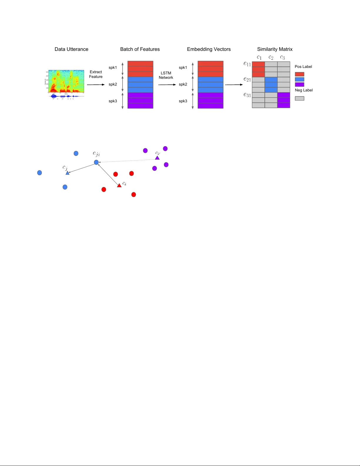
GENERALIZED END-TO-END LOSS FOR SPEAKER VERIFICA TION Li W an Quan W ang Alan P apir Ignacio Lopez Mor eno Google Inc., USA { liwan , quanw , papir , elnota } @google.com ABSTRA CT In this paper , we propose a new loss function called generalized end-to-end (GE2E) loss, which makes the training of speaker ver - ification models more efficient than our previous tuple-based end- to-end (TE2E) loss function. Unlike TE2E, the GE2E loss function updates the network in a w ay that emphasizes examples that are dif- ficult to verify at each step of the training process. Additionally , the GE2E loss does not require an initial stage of example selec- tion. W ith these properties, our model with the ne w loss function decreases speaker v erification EER by more than 10% , while reduc- ing the training time by 60% at the same time. W e also introduce the MultiReader technique, which allo ws us to do domain adaptation — training a more accurate model that supports multiple keywords ( i.e. , “OK Google” and “Hey Google”) as well as multiple dialects. Index T erms — Speaker verification, end-to-end loss, Multi- Reader , keyword detection 1. INTR ODUCTION 1.1. Background Speaker verification (SV) is the process of verifying whether an ut- terance belongs to a specific speaker , based on that speaker’ s kno wn utterances ( i.e. , enrollment utterances), with applications such as V oice Match [ 1 , 2 ]. Depending on the restrictions of the utterances used for enroll- ment and verification, speaker verification models usually fall into one of two categories: te xt-dependent speaker verification (TD-SV) and text-independent speaker verification (TI-SV). In TD-SV , the transcript of both enrollment and verification utterances is phone- tially constrained, while in TI-SV , there are no lexicon constraints on the transcript of the enrollment or verification utterances, expos- ing a larger v ariability of phonemes and utterance durations [ 3 , 4 ]. In this work, we focus on TI-SV and a particular subtask of TD-SV known as global passwor d TD-SV , where the verification is based on a detected keyw ord, e.g. “OK Google” [ 5 , 6 ] In previous studies, i-vector based systems have been the dom- inating approach for both TD-SV and TI-SV applications [ 7 ]. In recent years, more efforts ha ve been focusing on using neural net- works for speak er verification, while the most successful systems use end-to-end training [ 8 , 9 , 10 , 11 , 12 ]. In such systems, the neural network output vectors are usually referred to as embedding vectors (also kno wn as d-vectors ). Similarly to as in the case of i-vectors, such embedding can then be used to represent utterances in a fix di- mensional space, in which other, typically simpler, methods can be used to disambiguate among speakers. More information of this work can be found at: https://google. github.io/speaker- id/publications/GE2E 1.2. T uple-Based End-to-End Loss In our previous work [ 13 ], we proposed the tuple-based end-to- end (TE2E) model, which simulates the two-stage process of runtime enrollment and verification during training. In our ex- periments, the TE2E model combined with LSTM [ 14 ] achieved the best performance at the time. For each training step, a tu- ple of one e valuation utterance x j ∼ and M enrollment utter- ances x km (for m = 1 , . . . , M ) is fed into our LSTM network: { x j ∼ , ( x k 1 , . . . , x kM ) } , where x represents the features (log-mel- filterbank ener gies) from a fixed-length segment, j and k represent the speakers of the utterances, and j may or may not equal k . The tuple includes a single utterance from speaker j and M different utterance from speaker k . W e call a tuple positi ve if x j ∼ and the M enrollment utterances are from the same speaker , i.e. , j = k , and neg ativ e otherwise. W e generate positive and negati ve tuples alternativ ely . For each input tuple, we compute the L2 normalized response of the LSTM: { e j ∼ , ( e k 1 , . . . , e kM ) } . Here each e is an em- bedding vector of fixed dimension that results from the sequence- to-vector mapping defined by the LSTM. The centroid of tuple ( e k 1 , . . . , e kM ) represents the voiceprint built from M utterances, and is defined as follows: c k = E m [ e km ] = 1 M M X m =1 e km . (1) The similarity is defined using the cosine similarity function: s = w · cos( e j ∼ , c k ) + b, (2) with learnable w and b . The TE2E loss is finally defined as: L T ( e j ∼ , c k ) = δ ( j, k )  1 − σ ( s )  +  1 − δ ( j, k )  σ ( s ) . (3) Here σ ( x ) = 1 / (1 + e − x ) is the standard sigmoid function and δ ( j, k ) equals 1 if j = k , otherwise equals to 0 . The TE2E loss function encourages a larger value of s when k = j , and a smaller value of s when k 6 = j . Consider the update for both positiv e and negati ve tuples — this loss function is very similar to the triplet loss in FaceNet [ 15 ]. 1.3. Overview In this paper, we introduce a generalization of our TE2E architecture. This ne w architecture constructs tuples from input sequences of v ar- ious lengths in a more ef ficient way , leading to a significant boost of performance and training speed for both TD-SV and TI-SV . This paper is or ganized as follows: In Sec. 2.1 we give the definition of the GE2E loss; Sec. 2.2 is the theoretical justification for why GE2E updates the model parameters more effecti vely; Sec. 2.3 introduces a technique called “MultiReader”, which enables us to train a single model that supports multiple ke ywords and languages; Finally , we present our experimental results in Sec. 3 . 2. GENERALIZED END-TO-END MODEL Generalized end-to-end (GE2E) training is based on processing a large number of utterances at once, in the form of a batch that con- tains N speakers, and M utterances from each speaker in a verage, as is depicted in Figure 1 . 2.1. T raining Method W e fetch N × M utterances to build a batch. These utterances are from N different speakers, and each speaker has M utterances. Each feature vector x j i ( 1 ≤ j ≤ N and 1 ≤ i ≤ M ) represents the features extracted from speaker j utterance i . Similar to our previous work [ 13 ], we feed the features extracted from each utterance x j i into an LSTM netw ork. A linear layer is connected to the last LSTM layer as an additional transformation of the last frame response of the network. W e denote the output of the entire neural network as f ( x j i ; w ) where w represents all parameters of the neural network (including both, LSTM layers and the linear layer). The embedding vector (d-vector) is defined as the L2 normalization of the network output: e j i = f ( x j i ; w ) || f ( x j i ; w ) || 2 . (4) Here e j i represents the embedding vector of the j th speaker’ s i th ut- terance. The centroid of the embedding vectors from the j th speaker [ e j 1 , . . . , e j M ] is defined as c j via Equation 1 . The similarity matrix S j i,k is defined as the scaled cosine simi- larities between each embedding vector e j i to all centroids c k ( 1 ≤ j, k ≤ N , and 1 ≤ i ≤ M ): S j i,k = w · cos( e j i , c k ) + b, (5) where w and b are learnable parameters. W e constrain the weight to be positi ve w > 0 , because we want the similarity to be lar ger when cosine similarity is larger . The major difference between TE2E and GE2E is as follows: • TE2E’ s similarity (Equation 2 ) is a scalar value that defines the similarity between embedding vector e j ∼ and a single tuple centroid c k . • GE2E builds a similarity matrix (Equation 5 ) that defines the similarities between each e j i and all centroids c k . Figure 1 illustrates the whole process with features, embedding vec- tors, and similarity scores from dif ferent speakers, represented by different colors. During the training, we want the embedding of each utterance to be similar to the centroid of all that speaker’ s embeddings, while at the same time, far from other speakers’ centroids. As shown in the similarity matrix in Figure 1 , we w ant the similarity v alues of colored areas to be large, and the values of gray areas to be small. Figure 2 illustrates the same concept in a dif ferent way: we want the blue embedding v ector to be close to its own speaker’ s centroid (blue triangle), and far from the others centroids (red and purple triangles), especially the closest one (red triangle). Giv en an embedding vector e j i , all centroids c k , and the corresponding similarity matrix S j i,k , there are two ways to implement this concept: Softmax W e put a softmax on S j i,k for k = 1 , . . . , N that makes the output equal to 1 iff k = j , otherwise makes the out- put equal to 0 . Thus, the loss on each embedding vector e j i could be defined as: L ( e j i ) = − S j i,j + log N X k =1 exp( S j i,k ) . (6) This loss function means that we push each embedding vector close to its centroid and pull it away from all other centroids. Contrast The contrast loss is defined on positi ve pairs and most aggressiv e negativ e pairs, as: L ( e j i ) = 1 − σ ( S j i,j ) + max 1 ≤ k ≤ N k 6 = j σ ( S j i,k ) , (7) where σ ( x ) = 1 / (1 + e − x ) is the sigmoid function. For ev ery utter- ance, e xactly two components are added to the loss: (1) A positiv e component, which is associated with a positiv e match between the embedding vector and its true speaker’ s voiceprint (centroid). (2) A har d negati ve component, which is associated with a negati ve match between the embedding vector and the v oiceprint (centroid) with the highest similarity among all false speakers. In Figure 2 , the positi ve term corresponds to pushing e j i (blue circle) towards c j (blue triangle). The negativ e term corresponds to pulling e j i (blue circle) a way from c k (red triangle), because c k is more similar to e j i compared with c k 0 . Thus, contrast loss allows us to focus on difficult pairs of embedding vector and negati ve centroid. In our experiments, we find both implementations of GE2E loss are useful: contrast loss performs better for TD-SV , while softmax loss performs slightly better for TI-SV . In addition, we observed that removing e j i when computing the centroid of the true speaker makes training stable and helps avoid trivial solutions. So, while we still use Equation 1 when calculating negati ve similarity ( i.e. , k 6 = j ), we instead use Equation 8 when k = j : c ( − i ) j = 1 M − 1 M X m =1 m 6 = i e j m , (8) S j i,k = ( w · cos( e j i , c ( − i ) j ) + b if k = j ; w · cos( e j i , c k ) + b otherwise . (9) Combining Equations 4 , 6 , 7 and 9 , the final GE2E loss L G is the sum of all losses ov er the similarity matrix ( 1 ≤ j ≤ N , and 1 ≤ i ≤ M ): L G ( x ; w ) = L G ( S ) = X j,i L ( e j i ) . (10) 2.2. Comparison between TE2E and GE2E Consider a single batch in GE2E loss update: we ha ve N speakers, each with M utterances. Each single step update will push all N × M embedding vectors tow ard their own centroids, and pull them away the other centroids. This mirrors what happens with all possible tuples in the TE2E loss function [ 13 ] for each x j i . Assume we randomly choose P utterances from speaker j when comparing speakers: 1. Positive tuples: { x j i , ( x j,i 1 , . . . , x j,i P ) } for 1 ≤ i p ≤ M and p = 1 , . . . , P . There are  M P  such positiv e tuples. Extract Feature spk1 spk2 spk3 spk1 spk2 spk3 Similarity Matrix LSTM Network Embedding Vectors Batch of Features Data Utterance Pos Label Neg Label Fig. 1 . System ov erview . Different colors indicate utterances/embeddings from dif ferent speakers. Fig. 2 . GE2E loss pushes the embedding to wards the centroid of the true speaker , and away from the centroid of the most similar different speaker . 2. Negativ e tuples: { x j i , ( x k,i 1 , . . . , x k,i P ) } for k 6 = j and 1 ≤ i p ≤ M for p = 1 , . . . , P . For each x j i , we hav e to compare with all other N − 1 centroids, where each set of those N − 1 comparisons contains  M P  tuples. Each positi ve tuple is balanced with a ne gati ve tuple, thus the to- tal number is the maximum number of positi ve and negativ e tuples times 2. So, the total number of tuples in TE2E loss is: 2 × max  M P ! , ( N − 1) M P !  ≥ 2( N − 1) . (11) The lower bound of Equation 11 occurs when P = M . Thus, each update for x j i in our GE2E loss is identical to at least 2( N − 1) steps in our TE2E loss. The abo ve analysis sho ws why GE2E up- dates models more ef ficiently than TE2E, which is consistent with our empirical observ ations: GE2E con verges to a better model in shorter time (See Sec. 3 for details). 2.3. T raining with MultiReader Consider the following case: we care about the model application in a domain with a small dataset D 1 . At the same time, we have a larger dataset D 2 in a similar , but not identical domain. W e want to train a single model that performs well on dataset D 1 , with the help from D 2 : L ( D 1 , D 2 ; w ) = E x ∈ D 1 [ L ( x ; w )] + α E x ∈ D 2 [ L ( x ; w )] . (12) This is similar to the re gularization technique: in normal regular - ization, we use α || w || 2 2 to regularize the model. But here, we use E x ∈ D 2 [ L ( x ; w )] for regularization. When dataset D 1 does not have sufficient data, training the netw ork on D 1 can lead to overfitting. Requiring the network to also perform reasonably well on D 2 helps to regularize the network. This can be generalized to combine K different, possibly ex- tremely unbalanced, data sources: D 1 , . . . , D K . W e assign a weight α k to each data source, indicating the importance of that data source. During training, in each step we fetch one batch/tuple of utterances from each data source, and compute the combined loss as: L ( D 1 , · · · , D K ) = P K k =1 α k E x k ∈ D k [ L ( x k ; w )] , where each L ( x k ; w ) is the loss defined in Equation 10 . 3. EXPERIMENTS In our experiments, the feature e xtraction process is the same as [ 6 ]. The audio signals are first transformed into frames of width 25ms and step 10ms. Then we extract 40-dimension log-mel-filterbank energies as the features for each frame. For TD-SV applications, the same features are used for both keyword detection and speak er verification. The keyword detection system will only pass the frames containing the k eyword into the speaker verification system. These frames form a fixed-length (usually 800ms) segment. For TI-SV applications, we usually extract random fixed-length segments after V oice Activity Detection (V AD), and use a sliding windo w approach for inference (discussed in Sec. 3.2 ) . Our production system uses a 3-layer LSTM with projec- tion [ 16 ]. The embedding v ector (d-vector) size is the same as the LSTM projection size. For TD-SV , we use 128 hidden nodes and the projection size is 64 . For TI-SV , we use 768 hidden nodes with projection size 256 . When training the GE2E model, each batch contains N = 64 speakers and M = 10 utterances per speak er . W e train the network with SGD using initial learning rate 0 . 01 , and decrease it by half ev ery 30M steps. The L2-norm of gradient is clipped at 3 [ 17 ], and the gradient scale for projection node in LSTM is set to 0 . 5 . Regarding the scaling factor ( w , b ) in loss function, we also observed that a good initial value is ( w , b ) = (10 , − 5) , and the smaller gradient scale of 0 . 01 on them helped to smooth con vergence. 3.1. T ext-Dependent Speaker V erification Though existing v oice assistants usually only support a single ke y- word, studies show that users prefer that multiple keywords are supported at the same time. For multi-user on Google Home, two keyw ords are supported simultaneously: “OK Google” and “Hey Google”. Enabling speaker verification on multiple keywords falls be- tween TD-SV and TI-SV , since the transcript is neither constrained T able 1 . MultiReader vs. directly mixing multiple data sources. T est data Mixed data MultiReader (Enroll → V erify) EER (%) EER (%) OK Google → OK Google 1.16 0.82 OK Google → Hey Google 4.47 2.99 Hey Google → OK Google 3.30 2.30 Hey Google → Hey Google 1.69 1.15 T able 2 . T ext-dependent speaker v erification EER. Model Embed Loss Multi A verage Architecture Size Reader EER (%) (512 , ) [ 13 ] 128 TE2E No 3.30 Y es 2.78 (128 , 64) × 3 64 TE2E No 3.55 Y es 2.67 (128 , 64) × 3 64 GE2E No 3.10 Y es 2.38 to a single phrase, nor completely unconstrained. W e solve this problem using the MultiReader technique (Sec. 2.3 ). MultiReader has a great advantage compared to simpler approaches, e.g. directly mixing multiple data sources together: It handles the case when different data sources are unbalanced in size. In our case, we hav e two data sources for training: 1) An “OK Google” training set from anonymized user queries with ∼ 150 M utterances and ∼ 630 K speakers; 2) A mixed “OK/Hey Google” training set that is manually collected with ∼ 1 . 2 M utterances and ∼ 18 K speakers. The first dataset is larger than the second by a factor of 125 in the number of utterances and 35 in the number of speakers. For ev aluation, we report the Equal Error Rate (EER) on four cases: enroll with either k eyw ord, and verify on either ke yword. All ev aluation datasets are manually collected from 665 speakers with an av erage of 4 . 5 enrollment utterances and 10 evaluation utterances per speaker . The results are shown in T able 1 . As we can see, Mul- tiReader brings around 30% relativ e improvement on all four cases. W e also performed more comprehensi ve ev aluations in a lar ger dataset collected from ∼ 83 K different speak ers and environmen- tal conditions, from both anonymized logs and manual collections. W e use an av erage of 7 . 3 enrollment utterances and 5 ev aluation utterances per speaker . T able 2 summarizes average EER for differ - ent loss functions trained with and without MultiReader setup. The baseline model is a single layer LSTM with 512 nodes and an em- bedding vector size of 128 [ 13 ]. The second and third rows’ model architecture is 3-layer LSTM. Comparing the 2nd and 3rd rows, we see that GE2E is about 10% better than TE2E. Similar to T able 1 , here we also see that the model performs significantly better with MultiReader . While not shown in the table, it is also worth noting that the GE2E model took about 60% less training time than TE2E. 3.2. T ext-Independent Speaker V erification For TI-SV training, we divide training utterances into smaller seg- ments, which we refer to as partial utterances. While we don’t require all partial utterances to be of the same length, all partial utterances in the same batch must be of the same length. Thus, for each batch of data, we randomly choose a time length t within [ lb, ub ] = [140 , 180] frames, and enforce that all partial utterances in that batch are of length t (as shown in Figure 3 ). spk1 spk2 spk3 Pool of Features spk1 spk2 spk3 Batch 1 Random Segment spk1 spk2 spk3 Batch 2 Fig. 3 . Batch construction process for training TI-SV models. … Run LSTM on each of these sliding windows Sliding window stride Sliding window length L2 normalize, then average to get embedding d-vectors Fig. 4 . Sliding window used for TI-SV . During inference time, for e very utterance we apply a sliding window of fixed size ( l b + ub ) / 2 = 160 frames with 50% overlap. W e compute the d-vector for each windo w . The final utterance-wise d-vector is generated by L2 normalizing the window-wise d-v ectors, then taking the element-wise av erge (as sho wn in Figure 4 ). Our TI-SV models are trained on around 36M utterances from 18K speakers, which are extracted from anonymized logs. For e val- uation, we use an additional 1000 speakers with in av erage 6.3 en- rollment utterances and 7.2 ev aluation utterances per speaker . T a- ble 3 shows the performance comparison between different train- ing loss functions. The first column is a softmax that predicts the speaker label for all speak ers in the training data. The second col- umn is a model trained with TE2E loss. The third column is a model trained with GE2E loss. As shown in the table, GE2E performs bet- ter than both softmax and TE2E. The EER performance improv e- ment is larger than 10% . In addition, we also observ ed that GE2E training was about 3 × faster than the other loss functions. T able 3 . T ext-independent speaker verification EER (%). Softmax TE2E [ 13 ] GE2E 4.06 4.13 3.55 4. CONCLUSIONS In this paper , we proposed the generalized end-to-end (GE2E) loss function to train speaker verification models more efficiently . Both theoretical and experimental results verified the advantage of this nov el loss function. W e also introduced the MultiReader technique to combine dif ferent data sources, enabling our models to support multiple ke ywords and multiple languages. By combining these two techniques, we produced more accurate speaker v erification models. 5. REFERENCES [1] Y ury Pinsky , “T omato, tomahto. Google Home now supports multiple users, ” https://www .blog.google/products/assistant/tomato-tomahto- google-home-now-supports-multiple-users, 2017. [2] Mihai Matei, “V oice match will allow Google Home to recognize your voice, ” https://www .androidheadlines.com/2017/10/voice-match- will-allow-google-home-to-recognize-your -voice.html, 2017. [3] T omi Kinnunen and Haizhou Li, “ An overvie w of text- independent speaker recognition: From features to supervec- tors, ” Speech communication , vol. 52, no. 1, pp. 12–40, 2010. [4] Fr ´ ed ´ eric Bimbot, Jean-Franc ¸ ois Bonastre, Corinne Fre- douille, Guillaume Gra vier , Ivan Magrin-Chagnolleau, Syl- vain Meignier , T ev a Merlin, Javier Ortega-Garc ´ ıa, Dijana Petrovska-Delacr ´ etaz, and Douglas A Re ynolds, “ A tutorial on text-independent speaker verification, ” EURASIP journal on applied signal pr ocessing , vol. 2004, pp. 430–451, 2004. [5] Guoguo Chen, Carolina Parada, and Geor g Heigold, “Small- footprint keyw ord spotting using deep neural networks, ” in Acoustics, Speech and Signal Pr ocessing (ICASSP), 2014 IEEE International Confer ence on . IEEE, 2014, pp. 4087– 4091. [6] Rohit Prabhav alkar, Raziel Alvarez, Carolina Parada, Preetum Nakkiran, and T ara N Sainath, “ Automatic gain control and multi-style training for robust small-footprint k eyword spotting with deep neural networks, ” in Acoustics, Speech and Signal Pr ocessing (ICASSP), 2015 IEEE International Conference on . IEEE, 2015, pp. 4704–4708. [7] Najim Dehak, Patrick J Kenn y , R ´ eda Dehak, Pierre Du- mouchel, and Pierre Ouellet, “Front-end factor analysis for speaker v erification, ” IEEE T ransactions on Audio, Speech, and Language Pr ocessing , vol. 19, no. 4, pp. 788–798, 2011. [8] Ehsan V ariani, Xin Lei, Erik McDermott, Ignacio Lopez Moreno, and Javier Gonzalez-Dominguez, “Deep neural net- works for small footprint text-dependent speaker verification, ” in Acoustics, Speech and Signal Pr ocessing (ICASSP), 2014 IEEE International Confer ence on . IEEE, 2014, pp. 4052– 4056. [9] Y u-hsin Chen, Ignacio Lopez-Moreno, T ara N Sainath, Mirk ´ o V isontai, Raziel Alvarez, and Carolina Parada, “Locally- connected and conv olutional neural networks for small foot- print speaker recognition, ” in Sixteenth Annual Confer ence of the International Speech Communication Association , 2015. [10] Chao Li, Xiaokong Ma, Bing Jiang, Xiangang Li, Xuewei Zhang, Xiao Liu, Y ing Cao, Ajay Kannan, and Zhenyao Zhu, “Deep speaker: an end-to-end neural speaker embedding sys- tem, ” CoRR , vol. abs/1705.02304, 2017. [11] Shi-Xiong Zhang, Zhuo Chen, Y ong Zhao, Jinyu Li, and Y i- fan Gong, “End-to-end attention based text-dependent speaker verification, ” CoRR , vol. abs/1701.00562, 2017. [12] Seyed Omid Sadjadi, Sriram Ganapathy , and Jason W . Pele- canos, “The IBM 2016 speaker recognition system, ” CoRR , vol. abs/1602.07291, 2016. [13] Georg Heigold, Ignacio Moreno, Samy Bengio, and Noam Shazeer , “End-to-end text-dependent speaker verification, ” in Acoustics, Speech and Signal Pr ocessing (ICASSP), 2016 IEEE International Confer ence on . IEEE, 2016, pp. 5115– 5119. [14] Sepp Hochreiter and J ¨ urgen Schmidhuber , “Long short-term memory , ” Neural computation , vol. 9, no. 8, pp. 1735–1780, 1997. [15] Florian Schroff, Dmitry Kalenichenko, and James Philbin, “Facenet: A unified embedding for face recognition and clus- tering, ” in Pr oceedings of the IEEE Conference on Computer V ision and P attern Recognition , 2015, pp. 815–823. [16] Has ¸ im Sak, Andre w Senior, and Franc ¸ oise Beaufays, “Long short-term memory recurrent neural network architectures for large scale acoustic modeling, ” in F ifteenth Annual Confer ence of the International Speech Communication Association , 2014. [17] Razvan Pascanu, T omas Mikolo v , and Y oshua Bengio, “Un- derstanding the exploding gradient problem, ” CoRR , vol. abs/1211.5063, 2012.