공간과 길이의 최적 분리: 피라미드 피벙 모순의 해법

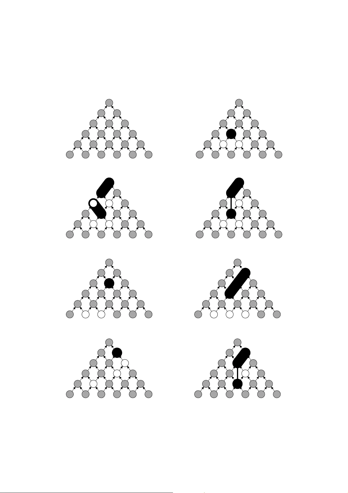
T o wards an Optimal Separation of Space and Length in Resolution ∗ Jakob Nordstr ¨ om † Johan H ˚ astad Royal Inst itute of T echno logy (KTH) SE-100 44 Stockho lm, Sweden { jakobn,jo hanh } @kth. se February 29, 2008 Abstract Most state-of-the- art satisfiability algorithms today are variants of the DPLL p rocedu re augmen ted with clause learnin g. The main bottlene ck for such algor ithms, other than the obvi- ous one of time, is the amou nt of memory used. In the field of proo f complexity , the resources of time and memory correspon d to the length and space of resolution proofs. Ther e has been a long line of research tryin g to understand these proof complexity measures, as well as relating them to the width of pro ofs, i.e., the size of the largest clau se in the proo f, which has been shown to be intimately conn ected with both length and space. While strong results ha ve been proven for length and width, ou r understan ding of space is still q uite poo r . For instance, it has remained open whether the fact that a formula is provable in short length implies that it is also provable in small space (which is the c ase for length versus width), or wh ether on the con- trary these measu res are completely unrelated in the sense tha t short proo fs can b e arbitrarily complex with respect to space. In this paper, we present som e e vid ence that the tr ue a nswer should be th at the latter c ase holds and provide a p ossible r oadmap for how such an optimal separation result could be ob- tained. W e d o this by p roving a tight bo und of Θ( √ n ) on the space n eeded for so-called pebbling contradictio ns over pyramid g raphs of size n . This yields the first p olynom ial lo wer bound on space that is not a conseq uence of a correspond ing lower bou nd on width, as well as an improvement of the weak separation of space and width in (Nordstr ¨ om 2 006) from log arith- mic to polyn omial. Also, continuin g the line of resear ch in itiated by ( Ben-Sasson 2 002) into trade-o ffs between different proo f co mplexity measur es, we p resent a simp lified proof of the recent len gth-space trade-off result in (Hertel and Pitassi 2 007), and show how our idea s can be u sed to prove a couple of other exponen tial trade-o ffs in resolu tion. 1 Introduc tion Ever since the fundame ntal NP -complet eness result o f Cook [21], th e prob lem of dec iding whether a gi ven prop ositional logic formula in conju nctiv e normal form (CNF) is sa tisfiable or not has been on center stage in Theoretical C omputer Science. In more recent years, S A T I S FI A B I L I T Y has gone from a problem of mainly theoretic al inte rest to a practical approach for solving applied problems. Although all kno wn Boolean satisfiabili ty solvers (SA T -solv ers) hav e ex ponential runnin g time in ∗ This is the full-length version of the paper [44] to appear at STOC ’08 . † Research supported in part by grants from the foundations Joha n och J akob S ¨ oderber gs sti ftelse and Sven och Dagmar Sal ´ ens stiftelse . TO W AR DS AN OPTIMAL SEP ARA TION the worst case , enormous progress in performance has led to satisfiability algorit hms becoming a standa rd tool for solv ing a lar ge number of real-world problems such as hardw are and softwar e ver ification, experimen t design, circuit diagno sis, and schedulin g. A some what surprising aspect of this dev elopment is that the most success ful SA T -solv ers to date are still varia nts of the resolu tion-based Dav is-Putnam-Logemann -Lovela nd (DPLL) proce- dure [25, 26] augmented with clause learnin g . For instan ce, the great majority of the best algo- rithms at the 2007 round of the interna tional SA T competi tions [53] fit this descripti on. DPLL proced ures perform a recursi ve backtrack search in the space of parti al truth value assignments. The idea b ehind clause learnin g, or confl ict-driven learning , is that at each f ailure (ba cktrack) point in the search tree, th e system deri ves a reaso n for the inc onsistenc y in the form of a ne w clause and then adds this clause to the original CNF formula (“learni ng” the clause). This can sa ve a lot of work later on in the proof search, when some other partial truth value assignment fails for similar reason s. The main bottlenec k for this approa ch, other than the obvi ous one of time, is the amount of memory used by the algorithms. Since there is only a finite amount of space, all clauses cannot be stored. The dif ficulty lies in obtainin g a highly selecti ve and efficient clause caching scheme that ne verthele ss keep s the clauses needed. Thus, understan ding time and m emory requiremen ts for clau se learning algorith ms, and ho w these requir ements are relat ed to one another , is a questi on of great practical importance. W e refer to, e.g., [9, 36, 51] for a more detaile d discussio n of claus e learnin g (and SA T -solvin g in general) with examples of appl ications. The stud y of proo f comple xity or iginated with the seminal paper of Cook and Reckho w [23]. In its most general form, a proof system for a language L is a predica te P ( x, π ) , computable in time polyn omial in | x | and | π | , such that for all x ∈ L there is a string π (a pr oof ) f or whi ch P ( x, π ) = 1 , whereas for any x 6∈ L it hold s for all strings π that P ( x, π ) = 0 . A proof system is said to be polyn omially bounded if for ev ery x ∈ L ther e is a proof π x of size at m ost polyno mial in | x | . A pr oposition al pr oof system is a proof system for the language of tautologies in propositio nal logic. From a theo retical point of vie w , one importan t moti vatio n for proo f complexit y is the inti mate conne ction with the fundamental q uestion of P versus NP . Since N P is ex actly the set of languages with po lynomially bounded proof syst ems, and since T AU T O L O G Y can be seen to be th e dual prob- lem of S A T I S FI A B I L I T Y , we ha ve the famou s theore m of [23] that NP = co - NP if and only if there exi sts a po lynomially bounded pro positional proof syste m. Thus, if it could be sho wn that there a re no polyno mially bounded proof systems for propositi onal tautologies , P 6 = NP woul d follo w as a coroll ary since P is closed under compl ement. O ne w ay of ap proaching this dis tant goal is to study strong er and stronger proof systems and try to prove superp olynomial lower bound s on proof size. Ho weve r , althoug h great progre ss has been made in the last couple of dec ades for a varie ty of proof systems, it seems that we are still very far from fully understandi ng the reasoning power of ev en quite simple ones. A second important moti vati on is that, as was mentioned abov e, designin g ef ficient algorithms for p roving ta utologies (or , equi vale ntly , testing satis fiability), is a v ery impor tant problem no t only in the theory of computat ion but also in appli ed research and industry . All automated theor em pro vers, regardle ss of whether they actually produce a w ritten proof, explicitly or implicitly define a system in which proofs are search ed for and rules which determine what proofs in this system look like. Proof complexity analyzes what it takes to simply w rite down and verify the proofs that such an automat ed theorem-pro ver might find, ig noring the computa tional effor t needed to actu ally find them. Thus a lower bound for a proof system tells us that any algorithm, e ven an optimal (non-d eterministic) one m aking all the right choices , must necessarily use at least the amount of a certain resource spec ified by this bound. In the other direction, theoretical upper bou nds on some proof comple xity measu re giv e us hope of finding good proof search algorithms with respect to this measure, prov ided that we can design algorithms that search for proofs in the system in an ef ficient manner . For DPLL procedu res with clause learning, the time and memory resources used are measured by the lengt h and space of proofs in the resolutio n proof system. 2 1 INTR ODUCT ION The field of proof complexi ty also has rich connectio ns to crypto graphy , artificial intelligen ce and mathematic al logic. Some good surve ys providin g more details are [7, 10, 54]. 1.1 Previous W ork Any formula in propositio nal logic can be con verted to a C NF formula that is only linearly lar ger and is unsatisfiab le if and only if the original formula is a tautology . Therefo re, any sound and complete syste m for refuting CNF formulas can be consider ed as a gener al proposi tional proof system. Perhaps the single most studied proof system in proposition al proof complex ity , r esolution , is such a system that produce s proofs of the unsati sfiability of CN F formulas. The resolutio n proof system appeared in [16] and began to be in vestig ated in connection w ith automated theorem provin g in the 1960s [2 5 , 26, 50]. Becaus e of its simplic ity—there is only one deriv ation rule—and becau se all lines in a proof are clause s, this proof system readily lends itself to proof search algorith ms. Being so simple and f undamental, resoluti on was also a natural tar get to attack when dev eloping methods for provin g lo wer bound s in proof complexity . In this contex t, it is m ost straigh tforward to pro ve bou nds on the le ngth of refutati ons, i.e., the number of cl auses, rather than on th e total size of refutations . T he length and size measu res are easil y seen to be poly nomially related. In 1968, Tseitin [58] present ed a superpolyn omial lower bound on refutat ion length for a restricted form of reso lution, called r e gular resolutio n, b ut it was not until almost 20 yea rs later that Hak en [32] pro ved the first superpolyn omial lo wer bound for general resoluti on. This weakly expone ntial bound of Haken has later been follo wed by many other strong results, among others truly expo- nentia l lower bound on resol ution refutatio n length for diff erent formula families in, for instance, [8, 15, 20, 59]. A second comple xity measure for resolution , fi rst made exp licit by Galil [30], is the width , measured as the max imal size of a clause in the re futation. Ben-Sasson and W igderson [15] sho wed that the minimal width W ( F ⊢ 0) of an y resolution refut ation of a k -CNF formula F is bounded from abo ve by the minimal refutation length L ( F ⊢ 0) by W ( F ⊢ 0) = O  p n log L ( F ⊢ 0)  , (1.1) where n is the number of variab les in F . Since it is also easy to see that resoluti on refuta- tions of polynomial-si ze formulas in small width must necess arily be short (for the reaso n that (2 · # v ariables ) w is an upper bound on the total number of distinct clause s of w idth w ), the result in [1 5 ] can be i nterpreted as say ing roughly that there e xists a sh ort refutatio n of the k -CN F formu- la F if and only if there exists a (reasona bly) narro w refutat ion of F . This gi ves rise to a natural proof se arch heurist ic: to find a short refuta tion, search for refutations in small width. It w as sho wn in [14] that there are formula fa milies for which this heuri stic expo nentially outperfo rms any DPLL proced ure regar dless of branching function. The formal study of space in resoluti on was initiated by E steban and T or ´ an [28, 56]. Intuiti vely , the space Sp ( π ) of a resolutio n refutatio n π is the maximal number of clause s one needs to keep in memory w hile verify ing the refutation, and the space Sp ( F ⊢ 0) of refuting F is defined as the minimal spa ce of any refutation of F . A number of upper and lower bounds for refutation space in resoluti on and other proof systems were subsequ ently presented in, for example, [2, 13, 27, 29]. Just as for width, t he minimum sp ace of refu ting a formul a can be u pper -bounded by the s ize of the formula. Somewhat unexpec tedly , howe ver , it also turned out that the lower bounds on resolutio n refutat ion space for se veral dif ferent formula families exact ly matched pre viously known lower bound s on refutation width . Atserias and D almau [5] showed that this was not a coinciden ce, bu t that the inequa lity W ( F ⊢ 0) ≤ Sp ( F ⊢ 0) + O(1) (1.2) 3 TO W AR DS AN OPTIMAL SEP ARA TION holds for any k -CN F formula F , where the (small) constant term depends on k . In [42], the first author prov ed that t he inequality (1.2) is asympto tically st rict by exhib iting a k -CNF formula family of size O( n ) refu table in width W ( F n ⊢ 0) = O(1) bu t requiring space Sp ( F n ⊢ 0) = Θ(log n ) . The space measure discussed abov e is known as clause space . A less well-studie d space mea- sure, introd uced by Alekhno vich et al. [2], is variable space , which counts the maximal number of v ariable occurrenc es that m ust be ke pt in memory simultaneousl y . Ben-Sasson [11] used this mea- sure to obt ain a trad e-off result for clause space ve rsus width in resol ution, proving that there are k -CNF formulas F n that can be refuted in constant clause space and constant width, but for which any refutation π n must ha ve Sp ( π n ) · W ( π n ) = Ω( n / log n ) . More recen tly , Hertel and Pitassi [33] sho wed that there are CNF formulas F n for which any refutation of F n in minimal variab le space V arSp ( F n ⊢ 0) must hav e expon ential length, but by adding just 3 extra units of storage one can instea d get a resoluti on refutation in linear length. 1.2 Questions Left Open by Pre vious Resear ch Despite all the research that has gone into understandi ng the resolution proof system, a number of fundame ntal questi ons still remain uns olved. W e touch briefly on two such questions belo w , and then discu ss a third one, which is the main focus of this paper , in somewha t more detail. Equation (1.1) says that short refuta tion lengt h implies narro w refutation w idth. Combining Equation (1.2) with the observ ation a bove that narro w ref utations a re tri vially short, we get a similar statemen t that small refutat ion clause space implies short refutation length. Note, ho wev er , that this does not mean that ther e is a refut ation that is bot h short and narr ow , or that any small-space refutat ion must also b e short . T he reason is that the resolutio n refutations on the left- and right-h and sides of (1.1) and (1.2) need not (and in genera l will not) be the same one. In view of the m inimum-width proof search heurist ic mentioned abov e, an important question is whether short refutation length of a formula does in fact entail that there is a refutation of it that is both short and narro w . Also, it would be int eresting to kno w if small spac e of a refuta tion implies that it is shor t. It is not kno wn whether there are such connect ions or whether on the contr ary there exi st some kind of trade-of f phenomena here similar to the one for space and width in [11]. A third, e ven more interesting problem is to clarify the relation between length and clause space. For width, rewritin g the bound in (1.1) in terms of the number of clauses | F n | instead of the number of v ariables we get that that if the width of refuting F n is ω  p | F n | log | F n |  , then the length of refuting F n must be superpoly nomial in | F n | . This is kno wn to be almost tight, sinc e [18] sho w s that there is a k - CNF formula fa mily { F n } ∞ n =1 with W ( F n ⊢ 0) = Ω  3 p | F n |  b ut L ( F n ⊢ 0) = O( | F n | ) . H ence, f ormula familie s refutable in p olynomial length can h av e some what wide minimum-width refuta tions, b ut not arb itrarily wide ones. What does t he correspo nding relation between space and l ength look lik e? The inequ ality (1.2) tells us that any correl ation between length and clause space cannot be tighter than the correlati on between length an d width, so in particular we get from th e p revio us paragraph that k -CNF formulas refutab le in polyno mial length may h av e at lea st “some what spaciou s” minimum-space refutati ons. At the other end of th e spec trum, giv en a ny resoluti on refutation π of F in leng th L it c an be prove n using results from [28, 34] that Sp ( π ) = O( L / log L ) . This gi ves an upper bound on any possible separa tion of the two measures. But is there a B en-Sasson –W igderson kind of upp er bound on space in terms of length similar to (1.1)? Or are length and space on the contrary unrelated in the sense that there exist k - CNF formulas F n with short refutati ons b ut maximal possible refutatio n space Sp ( F n ⊢ 0) = Ω  L ( F n ⊢ 0) / log L ( F n ⊢ 0)  in terms of length? W e note that for the restricted case of so-called tree-lik e resolutio n, [28] showed that there is a tight correspon dence between length and space, exac tly as for length versu s width . The case for genera l resolution has b een discusse d in, for i nstance, [11, 29, 57], b ut there se ems to ha ve bee n no consen sus on what the right answer should be. Howe ver , these papers identify a plausible formula 4 2 PR OOF O VER VIEW AND P APE R ORGA NIZA TION family for answering the questio n, namely so-cal led pebblin g contr adictio ns defined in terms of pebble games ov er directed acycli c graphs . 1.3 Our Contribution The main result in this paper provides some evide nce that the true answer to the questi on about the relations hip between space and length is m ore like ly to be at the latter extreme, i.e., that the two measu res can be separated in the strongest sense possible. More specifically , as a step tow ards reachi ng this goal we prov e an asymptotical ly tight bound on the clause space of refuting pebblin g contra dictions ov er pyramid graphs. Theor em 1.1. The clause space of r efuting pebbling contra dictions ove r pyramids of height h in r esolution gr ows as Θ ( h ) , pr ovided that the number of variables per vertex in the pebbli ng contr adiction s is at least 2 . This yields the first separat ion of space and lengt h (in the sens e of a poly nomial lower bound on space for formulas refu table in poly nomial length ) that is not a conseq uence of a correspon ding lo wer bound on width, as well as an e xponenti al improv ement of the separa tion of spa ce and w idth in [42]. Cor ollary 1.2. F or all k ≥ 4 , ther e is a family { F n } ∞ n =1 of k -C NF formulas of size Θ( n ) that can be re futed in r esolutio n in length L ( F n ⊢ 0) = O( n ) and width W ( F n ⊢ 0) = O(1) bu t r equir e clause space Sp ( F n ⊢ 0) = Θ( √ n ) . In addition to our m ain result, we also make the the observ ation that the proof of the recent trade-o ff result in [33] can be greatly simplified, and the parameters slightly improv ed. Using similar ideas, we can also prov e expo nential trade-of fs for length with respect to clause space and w idth. Namely , w e show tha t there are k -CNF formul as such that if we insist on finding the resolu tion refutation in smallest clause spac e or smallest width, respecti vel y , then w e hav e to pay with an exp onential increase in length. W e stat e the theor em only for length versu s clause space. Theor em 1.3. Ther e is a family of k -CNF formulas { F n } ∞ n =1 of size Θ( n ) suc h that: • The minimal clause space of r efuting F n in r esolut ion is Sp ( F n ⊢ 0) = Θ  3 √ n  . • Any res olution r efutation π : F n ⊢ 0 in m inimal clause space must have length L ( π ) = exp  Ω  3 √ n  . • Ther e ar e r esolut ion r efutation s π ′ : F n ⊢ 0 in a symptoticall y minimal clause space Sp ( π ′ ) = O  Sp ( F n ⊢ 0)  and length L ( π ′ ) = O( n ) , i.e ., linear in the formula size. A theor em of exactly the same form can be pro ven for length versu s width as well. 2 Proof Over vie w and Pa per Organization Since the proof of our main theorem is fa irly in v olved, w e start by gi ving an intuiti ve, high-l ev el descri ption of the proofs of our results and outlini ng how this pape r is orga nized. 2.1 Sketc h of Prelimi naries A r esolution r efutation of a CNF formula F can be vie wed as a sequence of deri vatio n steps on a blackb oard. In each step we may write a clau se from F on the blackbo ard (an axiom clause), erase a claus e from the blac kboard or deriv e some new clause implied by the clau ses curren tly written 5 TO W AR DS AN OPTIMAL SEP ARA TION on th e blackboar d. 1 The refu tation ends when we reach the cont radictory empty clause. The length of a resolution refutat ion is the number of distinct clause s in the refutat ion, the width is the size of the larg est clause in the refutati on, and the clause space is the maximum number of clauses on the blackb oard simultaneou sly . W e write L ( F ⊢ 0) , W ( F ⊢ 0) and Sp ( F ⊢ 0) to denote the minimum length , width and clause space, respecti vel y , of any resolu tion refutati on of F . The pebble g ame play ed on a directed acy clic graph (D A G) G models t he calcul ation described by G , where the source v ertices cont ain the input and non-s ource vertices spec ify operations on the v alues of the prede cessors. Placing a pebble on a vert ex v correspo nds to storing in memory the partial result of the calculation described by the subgraph rooted at v . Removing a peb ble from v corres ponds to deleting the partial result of v from memory . A pebbling of a DA G G is a seque nce of mov es startin g with the empty graph G and ending with all vertice s in G empty excep t for a pebble on the (unique ) sink ver tex. The cost of a pebblin g is the m aximal number of pebbles used simultan eously at any point in time during the pebbling . The pebbling price of a D AG G is the minimum co st of any pebblin g, i.e., the minimum number of memo ry registe rs require d to perform the complete calcula tion describ ed by G . The pebbl e game on a DA G G can be encod ed as an unsat isfiable CNF formula Peb d G , a so- called peb bling contradi ction of de gree d . See Figu re 1 for a small e xample. V ery br iefly , pebbling contra dictions are construct ed as follo ws: • Associate d v ariables x ( v ) 1 , . . . , x ( v ) d with each v ertex v (in Figure 1 we ha ve d = 2 ). • Specify that all so urces hav e at least one tru e varia ble, for example, the c lause x ( r ) 1 ∨ x ( r ) 2 for the verte x r in Figure 1. • Add clauses saying that truth prop agates from predecesso rs to successor s. For instanc e, for the verte x u with predecessor s r and s , clauses 4–7 in Figure 1 are the C NF encoding of the implicati on ( x ( r ) 1 ∨ x ( r ) 2 ) ∧ ( x ( s ) 1 ∨ x ( s ) 2 ) → ( x ( u ) 1 ∨ x ( u ) 2 ) . • T o get a contradict ion, conclude the formula with x ( z ) 1 ∧ · · · ∧ x ( z ) d where z is the sink of the D A G. W e will need the obser vatio n from [14] that a pebblin g contrad iction of degree d over a g raph with n v ertices can be refuted by resolution in length O  d 2 · n  and width O( d ) . 2.2 Pr oof I dea f or P ebbling Contradictions Space Bound Pebble games hav e been used extensi vel y as a tool to prov e time and space lo wer bounds and trade-o ffs for computation. Loosely put, a lower bound for the pebbling price of a graph says that althou gh the c omputation th at the graph describ es can b e p erformed quick ly , it r equires l arge space. Our hope is that w hen w e encode pebbl e games in terms of CNF formulas, these formulas inherit the same properties a s th e u nderlying grap hs. That is, if we pic k a D A G G with high pebbling price, since th e correspon ding pebbli ng contradictio n enc odes a calc ulation which requ ires large memory we would like to try to argue that an y resol ution refutati on of this formula shou ld require large space. Then a separati on result would follo w since we a lready kno w from [1 4] that the formula can be refuted in short length. More specifically , what we would like to do is to establi sh a connec tion betwee n re solution refu- tation s of pebbli ng contradictio ns on the o ne hand, and the so-called blac k-white pebble game [24] modellin g the non-deter ministic computation s describ ed by the unde rlying graphs on the other . Our intuitio n is that the resolu tion proof syste m should ha ve to conform to the combinat orics of the 1 For our proof, it turns out that the exact definition of the deriv ation rule is not essential—our lower bound holds for any sound rule. What is important is that we are only allo wed to d erive ne w clauses that are implied by the set of clauses currently on the blackboard. 6 2 PR OOF O VER VIEW AND P APE R ORGA NIZA TION ( x ( r ) 1 ∨ x ( r ) 2 ) ∧ ( x ( u ) 1 ∨ x ( v ) 1 ∨ x ( z ) 1 ∨ x ( z ) 2 ) ∧ ( x ( s ) 1 ∨ x ( s ) 2 ) ∧ ( x ( u ) 1 ∨ x ( v ) 2 ∨ x ( z ) 1 ∨ x ( z ) 2 ) ∧ ( x ( t ) 1 ∨ x ( t ) 2 ) ∧ ( x ( u ) 2 ∨ x ( v ) 1 ∨ x ( z ) 1 ∨ x ( z ) 2 ) ∧ ( x ( r ) 1 ∨ x ( s ) 1 ∨ x ( u ) 1 ∨ x ( u ) 2 ) ∧ ( x ( u ) 2 ∨ x ( v ) 2 ∨ x ( z ) 1 ∨ x ( z ) 2 ) ∧ ( x ( r ) 1 ∨ x ( s ) 2 ∨ x ( u ) 1 ∨ x ( u ) 2 ) ∧ x ( z ) 1 ∧ ( x ( r ) 2 ∨ x ( s ) 1 ∨ x ( u ) 1 ∨ x ( u ) 2 ) ∧ x ( z ) 2 ∧ ( x ( r ) 2 ∨ x ( s ) 2 ∨ x ( u ) 1 ∨ x ( u ) 2 ) ∧ ( x ( s ) 1 ∨ x ( t ) 1 ∨ x ( v ) 1 ∨ x ( v ) 2 ) ∧ ( x ( s ) 1 ∨ x ( t ) 2 ∨ x ( v ) 1 ∨ x ( v ) 2 ) ∧ ( x ( s ) 2 ∨ x ( t ) 1 ∨ x ( v ) 1 ∨ x ( v ) 2 ) ∧ ( x ( s ) 2 ∨ x ( t ) 2 ∨ x ( v ) 1 ∨ x ( v ) 2 ) z u v r s t Figure 1: The peb bling contradiction Peb 2 Π 2 fo r the pyramid g raph Π 2 of height 2. pebble game in the sense that from any resolution refutation of a pebblin g contra diction Peb d G we should be able to ex tract a pebbling of the D A G G . Ideally , we would like to gi ve a proof of a lower boun d on the resolution refutation space of pebbli ng contradi ctions along the follo wing lines: 1. First, find a natu ral interpretati on of sets o f clauses curre ntly “on the bl ackboard” in a refuta- tion of the formula Peb d G in terms of black and white pebble s on the vertic es of the D AG G . 2. Then, prove that this interpretati on of clau ses in terms of pebbles captures the pebble game in the follo wing sense: for any resolution refutati on of Peb d G , looking at consecuti ve sets of clause s on the blackb oard and consid ering the corres ponding sets of peb bles in the gra ph we get a black- white pebbling of G in accord ance with the rules of the pebble game. 3. Finally , sho w that the interp retation captures clause space in the sense tha t if the content of the blackb oard induces N pebb les on the graph, then there must be at least N clauses on the blackb oard. Combining the abov e with kno wn lower bound s on the pebblin g price of G , this would imply a lo wer bound on the refutatio n space of pebbling contradic tions and a separation from length and width. For c larity , let us spell out what the formal ar gument of this would look like. Consider an arbit rary resolution refutation of Peb d G . From th is refutation we extra ct a pebbling of G . At some poin t in time t in the obtaine d pebbling, there must be a lot of pebbles on the vert ices of G since thi s graph wa s chos en w ith high pebbli ng price. But th is means t hat at ti me t , th ere are a lot of clause s on the black board. Since this holds for any reso lution refutation, the refutation space of P eb d G must be l arge. The separa tion result now follows from the fact that pebbling contrad ictions are kno wn to be refutable in linear length and constant width if d is fixed. Unfortun ately , this idea does not quite work. In the next subsection , we describe the modifica- tions that we are forc ed to make, and show how we ca n mak e the bits an d piece s of our constr uction fit togethe r to yield Theorem 1.1 and Corollary 1.2 for the special case of pyra mid graphs . 7 TO W AR DS AN OPTIMAL SEP ARA TION           x ( u ) 1 ∨ x ( u ) 2 x ( s ) 1 ∨ x ( t ) 1 ∨ x ( v ) 1 ∨ x ( v ) 2 x ( s ) 1 ∨ x ( t ) 2 ∨ x ( v ) 1 ∨ x ( v ) 2 x ( s ) 2 ∨ x ( t ) 1 ∨ x ( v ) 1 ∨ x ( v ) 2 x ( s ) 2 ∨ x ( t ) 2 ∨ x ( v ) 1 ∨ x ( v ) 2           (a) Cl auses on black bo ard. z u v r s t (b) Co rrespond ing pebbles in the graph. Figure 2: Example of intuitiv e corr espondence between sets of clau s es and pebb les. 2.3 Detailed Overview of Formal Pr oof of Space Bound The black-whi te pebble game played o n a D A G G can be vie wed as a way of proving the end result of the calculation describ ed by G . Black pebbles denote proven partia l resu lts of the computation. White pebb les denot e assumptio ns about p artial resu lts which hav e been used to deri ve other partial results (i.e., black pebbles), but these assumptions w ill ha ve to be verified for the calculatio n to be complete. The final goal is a black pebble on the sink z and no other pebbles in the grap h, corres ponding to an uncond itional proof of the end result of the calculation with any assumptio ns made along the way ha ving been eliminate d. T ranslating this to pebbling contradicti ons, it turns out that a fruitfu l way to think of a black pebble on v is that it sh ould correspon d to truth o f the disju nction W d i =1 x ( v ) i of al l positi ve litera ls ov er v , or to “trut h of v ”. A white pebble on a verte x w can be understoo d to mean tha t we need to assume th e partial resul t on w to der iv e the black p ebbles abov e w in the graph . Needing to assume the truth of w is the oppo site of kno wing the truth of w , so extend ing the reasoning above we get that a w hite-p ebbled v ertex should correspond to “falsity of w ”, i.e., to all negati ve literals x ( w ) i , i ∈ [ d ] , over w . Using this intuit iv e corres pondence, we can transla te sets of clauses in a resol ution refutation of P eb d G into blac k and white pebbles in G as in Figure 2. It is easy to see that if we assume x ( s ) 1 ∨ x ( s ) 2 and x ( t ) 1 ∨ x ( t ) 2 , this assumption togethe r with the clauses on the blackbo ard in Figure 2(a) imply x ( v ) 1 ∨ x ( v ) 2 , so v shou ld be black-pebb led and s and t white-pebb led in Figure 2(b). T he ve rtex u is also black since x ( u ) 1 ∨ x ( u ) 2 certain ly is implied by the blackbo ard. This trans lation from clauses to pebbles is arg uably quite straightfo rward, and seems to yield well- beha ved black- white pebbling s for al l “sensible” resolution refutations of P eb d G . The problem is that we ha ve no guarante e that the resolu tion refutatio ns will be “sen sible”. Even though it might seem more or less clear ho w an optimal refutation of a pebbli ng contrad ic- tion should proceed, a particular refutatio n might contain unintuiti ve and seemingly non-optimal deri v ation steps that do not make much sense from a pebble game perspecti ve. In particular , a res- olutio n deri va tion has no obvi ous reaso n always to deriv e truth that is restricted to single verti ces. For instan ce, it could add the axioms x ( u ) i ∨ x ( v ) 2 ∨ x ( z ) 1 ∨ x ( z ) 2 , i = 1 , 2 , to the black board in Figure 2(a), deri ve that the truth of s and t implies the truth of either v or z , i.e., the clauses x ( s ) i ∨ x ( t ) j ∨ x ( v ) 1 ∨ x ( z ) 1 ∨ x ( z ) 2 for i, j = 1 , 2 , and then erase x ( u ) 1 ∨ x ( u ) 2 from th e black- board. Although it is hard to see from such a small example, this turns out to be a serious problem in that there appears to be no way that w e can interpret such deri v ation steps in terms of black and white pebble s without making some component in the proof idea in Section 2.2 break down. Instea d, w hat we do is to in vent a ne w pebb le game, with white pebbles just as before, bu t with black blobs that can cove r multiple vertic es instead of single-v ertex black pebbles. A blob on a verte x set V can be thought of as truth of some ver tex v ∈ V . T he deri va tion sketc hed in the preced ing paragraph, result ing in the se t of cla uses in Figur e 3(a), will th en be tra nslated into white 8 2 PR OOF O VER VIEW AND P APE R ORGA NIZA TION        x ( s ) 1 ∨ x ( t ) 1 ∨ x ( v ) 1 ∨ x ( z ) 1 ∨ x ( z ) 2 x ( s ) 1 ∨ x ( t ) 2 ∨ x ( v ) 1 ∨ x ( z ) 1 ∨ x ( z ) 2 x ( s ) 2 ∨ x ( t ) 1 ∨ x ( v ) 1 ∨ x ( z ) 1 ∨ x ( z ) 2 x ( s ) 2 ∨ x ( t ) 2 ∨ x ( v ) 1 ∨ x ( z ) 1 ∨ x ( z ) 2        (a) New set of clauses on blackboard. z u v r s t (b) Correspo nding blobs and pebbles. Figure 3: Intepreting sets of clauses as b lack b lobs and white pebbl es. pebble s on s and t as before and a b lack blob cov ering both v and z in Figure 3(b). W e define ru les in this blob-pebb le game corre sponding roughly to black and white pebble placement and remov al in the usual black-white pebble game, and add a speci al inflati on rule allowin g us to inflate black blobs to cov er more vertices . Once we ha ve this blob-peb ble game, we use it to construc t a lower bound proof as outlined in Section 2.2. First, we establish that for a fa irly general class of graphs , an y resolutio n refutation of a pebbling contradictio n can be interpreted as a blob-pebbl ing on the D A G in terms of which this pebbling contradic tion is defined. Intuiti vely , the reason that this works is that we can use the inflation rule to analy ze apparent ly non-optima l steps in the refutation. Theor em 2.1. Let Peb d G denote the pe bbling contr adiction of de gr ee d ≥ 1 over a layer ed D AG G . Then ther e is a translat ion function fr om sets of clauses derived fr om Peb d G into sets of blac k blobs and white pebb les in G such tha t any r esolution r efutation π of Peb d G corr esponds to a blob- pebbli ng P π of G unde r this transla tion. In fact, the only property that w e need from the layered graphs in T heorem 2.1 is that if w is a ver tex w ith predecess ors u and v , then there is no path between the siblings u and v . T he theorem holds for an y D A G satisfying this condition. Next, w e carefully design a cost function for black blobs and w hite pebbles so that the cost of the blob-p ebbling P π in Theorem 2.1 is related to the space of the resol ution refuta tion π . Theor em 2.2. If π is a re futation of a pebbling contrad iction Pe b d G of de gr ee d > 1 , then the cost of the assoc iated blob-peb bling P π is boun ded by the space of π by cost ( P π ) ≤ Sp ( π ) + O(1) . W ithout going into too much detail, in order to m ake the proof of Theorem 2.2 work we can only char ge for black blob s ha ving distin ct lowest vertices (measured in topol ogical order), so additional blobs with the same bottom vertice s are free. Also, we can only charge for white pebbles belo w these bottom vert ices. Finally , we need lower bounds on blob-pebbl ing price. B ecause of the inflati on rule in com- binati on with the peculiar cost function, the blob-pebble game seems to beh av e rather differe ntly from the standard black-white pebble game, and therefore we cannot appeal directly to kno wn lo wer bound s on bl ack-white pebbling price. Ho wev er , for a more res tricted class of graph s than in Theorem 2 .1, b ut still includ ing binary tre es and p yramids, we man age to pro ve ti ght bounds o n the blob-p ebbling price by gen eralizing the lower boun d constructi on for black-white pebblin g in [37]. Theor em 2.3. Any so-called layer ed s pr eading gr aph G h of height h has blob- pebbling price Θ( h ) . In parti cular , this holds for pyramid grap hs Π h . Putting all of this togethe r , we can prov e our m ain theore m. 9 TO W AR DS AN OPTIMAL SEP ARA TION Theor em 1.1 (r estated). Let Peb d Π h denote the pebblin g contr adiction of de gr ee d > 1 defined ove r the pyra mid graph of height h . Then the clause space of r efutin g P eb d Π h by r esoluti on is Sp ( Peb d Π h ⊢ 0) = Θ( h ) . Pr oof. The upper bound Sp ( Peb d Π h ⊢ 0) = O( h ) is easy . A pyramid of height h can be pebbled with h + O (1) black pebbles, and a resolution refutat ion can mimic such a pebbli ng in consta nt ext ra clause space (independe nt of d ) to ref ute the correspondi ng pebbl ing contradicti on. The interesting part is the lo wer bound. Let π be any resolutio n refutation of Peb d Π h . C on- sider the associa ted blob-p ebbling P π pro vided by Theorem 2.1. On the one hand, we kno w that cost ( P π ) = O( Sp ( π )) by Theorem 2.2 , provi ded that d > 1 . On the other hand, T heo- rem 2.3 tells us that the cost of any blob-peb bling of Π h is Ω( h ) , so in particular we must hav e cost ( P π ) = Ω( h ) . Combining these two bou nds on cost ( P π ) , we see that Sp ( π ) = Ω( h ) . The pebbling contradict ion P eb d G is a (2+ d )-C NF formula and for consta nt d the size of the formula is linear in the number of vert ices of G (compare F igure 1). T hus, for pyramid graphs Π h the corresp onding pebbl ing contrad ictions Peb d Π h ha ve size quadra tic in the height h . A lso, when d is fixed the upper bounds mentioned at the end of Section 2.1 become L ( Peb d G ⊢ 0) = O( n ) and W ( Pe b d G ⊢ 0) = O(1) . Corollary 1.2 now follo ws if we set F n = Peb d Π h for d = k − 2 and h = ⌊ √ n ⌋ and use T heorem 1.1. Cor ollary 1 .2 (r estated). F or all k ≥ 4 , ther e is a fa mily o f k -C NF formulas { F n } ∞ n =1 of size O( n ) suc h that L ( F n ⊢ 0) = O( n ) and W ( F n ⊢ 0) = O(1) b ut Sp ( F n ⊢ 0) = Θ( √ n ) . 2.4 Overview of T rade-off Results Let us also quickly sketch the ideas (or tricks, really) used to prove our trade-of f theorems for resolu tion. W e show the follo wing versio n of the leng th-va riable space trade-of f theorem of H ertel and Pitassi [33], with some what improve d parameters and a very much simpler proof. Theor em 2.4. Ther e is a family of C NF formul as { F n } ∞ n =1 of size Θ( n ) suc h that: • The minimal variable space of r efuting F n in r esolution is V arSp ( F n ⊢ 0) = Θ( n ) . • Any r esolution r efutation π : F n ⊢ 0 in minimal var iable space has leng th exp (Ω( √ n )) . • Adding at most 2 extr a units of stora ge , it is possible to obtain a re solution r efutati on π ′ in variab le space V arSp ( π ′ ) = V arSp ( F n ⊢ 0) + 3 = Θ( n ) and leng th L ( π ′ ) = O( n ) , i.e., linear in the formula size . The idea behi nd o ur proof is as follo ws. T ake formulas G n that are really hard for resolutio n and formulas H m which ha ve s hort refu tations b ut requ ire linear v ariable sp ace, and set F n = G n ∧ H m for m chosen so that V arSp  H m ⊢ 0  is only jus t lar ger than V arSp  G n ⊢ 0  . Then refutations in minimal v ariable space will ha ve to take ca re of G n , which requi res exponen tial length, b ut adding one or two litera ls to the memory we can attac k H m instea d in linear length. The trade-of f result in Theorem 1.3 for length versus clause space and its twin theorem for length ver sus w idth are sho w n using similar ideas. 2.5 P aper Organization Section 3 pro vides formal definitions of the conc epts introd uced in Sections 1 an d 2, and Section 4 gi ves precise statemen ts of the result s mentione d there, as well as some othe r result rele vant to this paper . The easy proof s of our trade-of f theorems are then immediately presented in Section 5. The b ulk of the paper is spent proving our main result in Theorem 1.1. In Section 6, we define our modified pebb le game, the “blob-p ebble game”, that w e will use to analyze reso lution 10 3 FORMAL PREL IMIN ARIES refutat ions of pebb ling contradictio ns. In Section 7 we pro ve that resoluti on refutation s can be transla ted into pebbli ngs in this game, which is Theorem 2.1 in Section 2.3. In Section 8, we pro ve Theorem 2.2 saying that the blob-pebbl ing price acc urately measures the clause space of the corres ponding resolution refutati on. Finally , after givi ng a detailed descrip tion of the lower bound on blac k-white pebblin g of [37] in Section 9 (with a somewhat simpli fied proof that might be of indepe ndent interest), in Section 10 we g eneralize this result in a n ontri vial way to ou r blob-pebbl e game. This giv es us Theorem 2.3. N o w Theorem 1.1 and Corollary 1.2 follo w as in the proofs gi ven at the end of Section 2.3. W e conclude in Section 11 by giv ing suggestion s for fu rther research. 3 Formal Preliminaries In this section , we define resoluti on, pebble games and pebbling contradic tions. 3.1 The Resolution Pr oof System A literal is either a propositio nal logic varia ble or its ne gation, denoted x and x , respecti vely . W e define x = x . T wo literals a and b are strictly distinct if a 6 = b and a 6 = b , i.e., if they refer to distin ct v ariables. A clause C = a 1 ∨ · · · ∨ a k is a s et of literals . Througho ut this pap er , all claus es C are assumed to be nontr ivial in the sense th at all literals in C are pairwise strictly dis tinct ( otherwise C is tri vially true). W e say that C is a subclause of D if C ⊆ D . A clause containin g at most k literals is called a k -clause . A CNF formula F = C 1 ∧ · · · ∧ C m is a set of clauses. A k -CN F formula is a CNF formula consis ting of k -clauses. W e define t he size S ( F ) of the fo rmula F to be the total number o f literals in F count ed w ith repet itions. More often, we will be in terested in the number of clauses | F | of F . In this pape r , when nothing else is stated it is assu med that A, B , C , D denote clause s, C , D sets of clauses , x, y propositio nal v ariables, a, b, c literals, α, β truth va lue assignments and ν a truth v alue 0 or 1 . W e write α x = ν ( y ) = ( α ( y ) if y 6 = x , ν if y = x , (3.1) to denote the truth valu e assignment that agrees with α eve rywhere except possibly at x , to which it assigns the va lue ν . W e let V ars ( C ) denote the set of var iables and Lit ( C ) the set of literals in a claus e C . 2 This nota tion is exte nded to sets of clauses by taki ng unions . Also, we emplo y the standa rd notation [ n ] = { 1 , 2 , . . . , n } . A r esolutio n derivatio n π : F ⊢ A of a clause A from a CNF formula F is a sequen ce of cla uses π = { D 1 , . . . , D τ } such that D τ = A and each line D i , i ∈ [ τ ] , either is one of the clauses in F ( axioms ) or is deri ved from clauses D j , D k in π with j, k < i by the r esolutio n rule B ∨ x C ∨ x B ∨ C . (3.2) W e refer to (3.2) as r esolutio n on the variable x and to B ∨ C as the r esolvent of B ∨ x and C ∨ x on x . A r esoluti on r efutati on of a CNF formula F is a resolut ion deri vation of the empty clause 0 (the clause with no litera ls) from F . Perhaps s omewhat confu singly , this is sometimes also referred to as a r esoluti on pr oof of F . For a formula F and a set of formula s G = { G 1 , . . . , G n } , w e say that G implies F , den oted G  F , if eve ry truth value assignment satisfying all formulas G ∈ G satisfies F as well. It is 2 Although t he notation Lit ( C ) is slightly redundant giv en the definition of a clause as a set of lit erals, we include it for clarity . 11 TO W AR DS AN OPTIMAL SEP ARA TION well kno wn that resolutio n is soun d and implication ally complete. That is, if there is a resol ution deri v ation π : F ⊢ A , then F  A , and if F  A , then there is a resol ution deriv ation π : F ⊢ A ′ for some A ′ ⊆ A . In particular , F is unsatisfiable if and only if there is a resolution refutation of F . W ith e very resolu tion deri va tion π : F ⊢ A we can associat e a D A G G π , with the clauses in π labelli ng the vertice s and with edg es from the ass umption clauses to the reso lvent for each app lica- tion of th e resolution rule (3.2). There might be se ver al diffe rent deriv ations of a clause C in π , bu t if so we can label each occurrence of C with a timesta mp when it was deriv ed and keep track of which cop y of C is used where. A resolutio n deri va tion π is tr ee-like if an y clause in the deri vat ion is used at most once as a premise in an application of the resolut ion rule, i.e., if G π is a tree. (W e may make diff erent “time-sta mped” v ertex copies of the axiom clauses in order to make G π into a tree). The length L ( π ) of a re solution deri v ation π is the number of clause s in it. W e define th e leng th of deriv ing a clause A from a formula F as L ( F ⊢ A ) = min π : F ⊢ A { L ( π ) } , where the minimum is taken ove r all resolution deriv ations of A . In particular , the length of refuting F by resolution is denote d L ( F ⊢ 0) . T he le ngth of refuting F by tree-lik e resolution L T ( F ⊢ 0) is define d by takin g the minimum ov er all tree-lik e resoluti on refutatio ns π T of F . The w idth W ( C ) of a clause C is | C | , i.e., the number of literal s appearing in it. The width of a set of clauses C is W ( C ) = max C ∈ C { W ( C ) } . The width of deriv ing A from F by resolution is W ( F ⊢ A ) = min π : F ⊢ A { W ( π ) } , and the width of refuti ng F is denoted W ( F ⊢ 0) . Note that the minimum w idth measures in general and tree-lik e resoluti on coincide , so it makes no sense to make a sepa rate definition for W T ( F ⊢ 0) . W e nex t define the measure of space . Follo wing the expos ition in [28], a proof can be seen as a Tur ing machine computation, with a special read-only input tape from which the axioms can be do wnloaded and a working memory where all deri vati on steps are made. The clause space of a resolu tion proof is th e maximum numb er of claus es that need to be k ept in memor y simultane ously during a ve rification of the proof. T he variabl e space is the maximum total spac e needed, where also the width of the clause s is taken into accoun t. For the formal definitions , it is con ven ient to use an alterna tiv e definition of resoluti on intro - duced in [2]. Definition 3.1 (Resolutio n). A clause configu ration C is a set of clauses. A sequ ence of claus e configura tions { C 0 , . . . , C τ } is a r esolution der ivation from a CNF formula F if C 0 = ∅ and for all t ∈ [ τ ] , C t is obtai ned from C t − 1 by one 3 of the follo wing rules: Axiom Do wn load C t = C t − 1 ∪ { C } for some C ∈ F . Erasure C t = C t − 1 \ { C } for some C ∈ C t − 1 . Infere nce C t = C t − 1 ∪ { D } for some D inferred by resolutio n from C 1 , C 2 ∈ C t − 1 . A resolu tion deri vati on π : F ⊢ A of a clause A from a formula F is a deri vatio n { C 0 , . . . , C τ } such that C τ = { A } . A re solution ref utation of F is a deri vat ion of the empty clause 0 from F . Definition 3.2 (Clause sp ace [2, 11]). The clause space of a resolutio n deri vation π = { C 0 , . . . , C τ } is max t ∈ [ τ ] {| C t |} . The clau se space of deriv ing A from F is Sp ( F ⊢ A ) = min π : F ⊢ A { Sp ( π ) } , and Sp ( F ⊢ 0) denot es the minimum clause space of any resolu tion refutat ion of F . Definition 3.3 (V ariable space [2]). The variable space of a configuratio n C is V arSp ( C ) = P C ∈ C W ( C ) . The vari able space of a deriv ation { C 0 , . . . , C τ } is max t ∈ [ τ ] { V arSp ( C t ) } , and V arSp ( F ⊢ 0) is the minimum vari able space of any r esolution refutation of F . 3 In some pre vious pap ers, resolution is defined so as to allow ev ery deriv ation step to combine one or zero app lications of each of the three deriv ation r ules. Therefore, some of the bounds st ated in this paper for space as defined next are off by a constant as compared to the cited sources. 12 3 FORMAL PREL IMIN ARIES Restricti ng the resolutio n deri vatio ns to tree-li ke resolu tion, we get the measures Sp T ( F ⊢ 0) and V arSp T ( F ⊢ 0) in analo gy with L T ( F ⊢ 0) defined abo ve. Note that if one wanted to be really precise, the size and space measures should probably measure the number of bits needed rather than the number of literals. Howe ver , counting literals makes matters substan tially cleaner , and the dif ference is at most a logarithmic factor anywa y . Therefore , counting lite rals seems to be the es tablished way of measu ring formula size a nd v ariable space. In this paper , we will be almost exclusi vel y inte rested in the clause space of general resolution refutat ions. When we write simply “space” for bre vity , we mean clause space. 3.2 P ebble Games and P ebbling Contradictions Pebble games were de vised for studying programming language s and compiler constructi on, bu t ha ve found a varie ty of applica tions in computation al complex ity theory . In conne ction with reso- lution , pebble games hav e been employ ed bo th t o analy ze reso lution de riv ations with respect to how much memory they consume (using the origina l definition of space in [28]) and to construct C NF formulas w hich are hard for diff erent varia nts of resolution in vario us resp ects (see for example [3, 14, 17, 19]). An e xcellent survey of pe bbling up to ca 1980 is [48]. The black pebb ling price of a D A G G capture s the memory sp ace, i.e., the number of reg isters, requir ed to perform the deter ministic computati on des cribed by G . The space of a non-determini stic computa tion is measured by the black-white pebblin g price of G . W e say that vertic es of G with inde gree 0 are sour ces and that vertices with outde gree 0 are sinks or tar gets . In the follo wing, unless otherwise stated we will assu me that all D A Gs under discussion ha ve a unique sink and this sink will always be denoted z . The nex t definition is adapted from [24], though we use the establ ished pebbling terminology introduc ed by [34]. Definition 3 .4 (P ebble ga me). S uppose t hat G is a D A G with sources S and a unique tar get z . T he blac k-white pebb le game on G is the followin g one-playe r game. A t any point in the game, there are blac k and white pebbl es placed on s ome vertices of G , at mos t one pebble per v ertex. A p ebble config uration is a pair of subsets P = ( B , W ) of V ( G ) , comprising the black-pebb led vert ices B and white-pe bbled vertic es W . T he rules of the game are as foll ows: 1. If all imm ediate prede cessors of an empty verte x v ha ve pebbles o n them, a b lack peb ble may be placed on v . In particul ar , a black pebble can always be place d on any v ertex in S . 2. A black pebble may be remov ed from any ver tex at any time. 3. A white pebble may be placed on any empty ve rtex at any time. 4. If all immediate predec essors of a white-pebble d verte x v hav e pebbles on them, the w hite pebble on v may be remov ed. In particular , a white pebb le can always be removed from a source ver tex. A blac k-white peb bling from ( B 1 , W 1 ) to ( B 2 , W 2 ) in G is a seque nce of p ebble co nfigurations P = { P 0 , . . . , P τ } such that P 0 = ( B 1 , W 1 ) , P τ = ( B 2 , W 2 ) , and for all t ∈ [ τ ] , P t follo ws from P t − 1 by one of the rules abo ve. If ( B 1 , W 1 ) = ( ∅ , ∅ ) , we say that the pebbling is unco nditional , otherwis e it is conditio nal . The cost of a pebble configuratio n P = ( B , W ) is cost ( P ) = | B ∪ W | and the cost of a pebbli ng P = { P 0 , . . . , P τ } is max 0 ≤ t ≤ τ { cost ( P t ) } . The blac k-white pebbling price of ( B , W ) , denote d BW -P eb ( B , W ) , is the minimum cost of any unco nditional pebbling reaching ( B , W ) . A complete pebbling of G , also called a pebbling strate gy for G , is an unconditi onal pebbling reachi ng ( { z } , ∅ ) . The blac k-white pebb ling price of G , denoted BW -P eb ( G ) , is the m inimum cost of any co mplete black-white pebbling of G . 13 TO W AR DS AN OPTIMAL SEP ARA TION A blac k pebbli ng is a pebbli ng usin g black pebbles only , i.e., ha ving W t = ∅ for all t . The (blac k) pebb ling price of G , den oted P eb ( G ) , is the minimum c ost of an y complete b lack pebb ling of G . W e think of the mo ves in a p ebbling as occur ring at integra l time interv als t = 1 , 2 , . . . and talk about the pe bbling move “a t time t ” (which is the mo ve resu lting in configuration P t ) or th e moves “durin g the time interv al [ t 1 , t 2 ] ”. The only peb blings we are re ally interest ed in are comple te pebblings of G . H o weve r , when we pro ve lo wer bou nds for pe bbling price i t will so metimes be con venien t to be able to r eason in te rms of parti al pebbli ng move s equences, i.e., conditiona l peb blings. A pebbling cont radictio n defined on a D A G G encodes the pebbl e game on G by postula ting the source s to be true and the targe t to be false, and specifying that truth propagates through the graph accord ing to the pebbling rules. T he definition belo w is a generalizat ion of formulas previo usly studie d in [17, 49]. Definition 3.5 (Pebbling contradictio n [15]). S uppose that G is a D A G with sources S , a unique tar get z and with all non-so urce vertic es ha ving indegre e 2 , and let d > 0 be an integer . A sso- ciate d distinc t vari ables x ( v ) 1 , . . . , x ( v ) d with ev ery verte x v ∈ V ( G ) . The d th deg ree pebblin g contr adiction ove r G , denoted Peb d G , is the conjun ction of the follo wing clauses: • W d i =1 x ( s ) i for all s ∈ S ( sour ce axioms ), • x ( z ) i for all i ∈ [ d ] ( tar get axioms ), • x ( u ) i ∨ x ( v ) j ∨ W d l =1 x ( w ) l for all i, j ∈ [ d ] and all w ∈ V ( G ) \ S , w here u, v are the two predec essors of w ( pebbl ing axioms ). The formula Peb d G is a (2+ d )-CNF formula with O  d 2 · | V ( G ) |  clause s o ver d · | V ( G ) | va ri- ables. An ex ample pebbling contradictio n is presented in Figure 1 on page 7. 4 Re vie w of Related W ork This section is a n o vervie w of relate d work, i ncluding formal statemen ts of some pre viously kno wn results that we will need. At the end of Section 4.3 we also try to prov ide some of the intuitio n behind the result prov en in this paper . 4.1 General Results About Resolution It is not hard to sho w that any CNF formula F over n variab les is refutab le in length 2 n +1 − 1 and width n . Esteban a nd T or ´ an [28] p rove d that the clause s pace of refuting F is upper -bounded by t he formula size. More precisely , the minimal clause space is at most the number of clauses, or the num- ber o f v ariables, plus a small consta nt, or in formal notatio n Sp ( F ⊢ 0) ≤ min  | F | , | V ars ( F ) |  + O(1) . W e will need the fact that there are polynomial-si ze familie s of k -CNF formulas that are very hard with respect to length, w idth and clause space, essent ially meeting the upper bounds just stated . Theor em 4.1 ([2, 8, 13, 15, 20, 56, 59]). The re ar e arbit rarily lar ge unsatisfia ble 3 -CNF formu- las F n of size Θ( n ) with Θ( n ) clau ses and Θ ( n ) variables for which it holds that L ( F n ⊢ 0) = exp(Θ( n )) , W ( F n ⊢ 0) = Θ( n ) and Sp ( F n ⊢ 0) = Θ( n ) . 14 4 REVIEW OF RELA TED W ORK Clearly , for such formulas F n it must also hold that Ω( n ) = V arSp ( F n ⊢ 0) = O  n 2  . W e note in passing that determinin g the exa ct va riable space complex ity of a formula family as in Theorem 4.1 was mention ed as an open problem in [2]. T o the best of our knowle dge this problem is still unsolv ed. If a reso lution refuta tion has constan t width, it is easy to see that it must be of si ze p olynomial in the numbe r of v ariables (just coun t the maximum poss ible number of di stinct clauses) . Con verse ly , if all refutation s of a formula are very wide, it seems reasonable that any refutati on of this formula must be ver y long as well. This i ntuition was made pr ecise by Ben-Sasson and W igders on [15]. W e state their theorem in the more exp licit form of Segerlind [54]. Theor em 4.2 ([15]). The width of r efuting a CNF formula F is boun ded fr om above by W ( F ⊢ 0) ≤ W ( F ) + 1 + 3 p n ln L ( F ⊢ 0) , wher e n is the number of varia bles in F . Bonet and G alesi [18] sho wed that this bound on width in te rms of leng th is essentially optima l. For the special case of tree-lik e reso lution, ho wev er , it is possible get rid of the depende nce of the number of v ariables and obtain a tighter bound. Theor em 4.3 ([15]). The wid th o f r efuting a CNF formula F in tr ee-like r esoluti on is bound ed fr om abo ve by W ( F ⊢ 0) ≤ W ( F ) + log L T ( F ⊢ 0) . For refe rence, we collect the result in [18] together with some other bounds showing that there are formulas that are easy with respect to length bu t moderat ely hard with respect to width and clause space and state them as a theore m. 4 Theor em 4.4 ([2, 18 , 55]). T her e ar e arbitr arily lar ge unsatisfiab le 3 -CNF formulas F n of size Θ  n 3  with Θ  n 3  clause s and Θ  n 2  variab les such that W ( F n ⊢ 0) = Θ( n ) and Sp ( F n ⊢ 0) = Θ( n ) , b ut for which ther e ar e r esolutio n refu tations π n : F n ⊢ 0 in length L ( π n ) = O  n 3  , width W ( π n ) = O( n ) and clause space Sp ( π n ) = O( n ) . As was mentioned abov e, the fa ct that all known lo wer boun ds on refutation clau se space co- incide d with lo wer bounds on width lead to the conjectu re that the width measure is a lo wer bound for the clause space measure. This con jecture was pro ven true by Atserias and Dalmau [5]. Theor em 4.5 ([5]). F or any CNF formula F , it holds that Sp ( F ⊢ 0) − 3 ≥ W ( F ⊢ 0) − W ( F ) . In other words , the ext ra clause space exc eeding the minimum 3 needed for any resolution deri v ation is boun ded from belo w by the extra width ex ceeding the w idth of the formula. This inequa lity was later sho wn by the first author to be asymptotica lly strict in the followin g sense. Theor em 4.6 ([42]). F or all k ≥ 4 , ther e is a family { F n } ∞ n =1 of k -CN F formula s of size Θ( n ) suc h that L ( F n ⊢ 0) = O( n ) and W ( F n ⊢ 0) = O(1) b ut Sp ( F n ⊢ 0) = Θ(log n ) . An immediate coro llary of Theorem 4.5 is that for polynomial -size k -CNF formul as constant clause space implies polyno mial proof length. W e are interes ted in finding out w hat holds in the other directio n, i.e., if upper bounds on length imply upper bounds on space. For the special case of tree-lik e resolution, it is kno w n that there is an upper bound on clau se space in terms of lengt h exac tly analogous to the one on width in terms of length in Theorem 4.3. 4 Note t hat [18], where an explicit resolution refutation upper-bound ing the proof complexity measures is presented, does not talk about clause space, but it is straightforward to verify that the refutation there can be carried out in length O ` n 3 ´ and clause space O( n ) . 15 TO W AR DS AN OPTIMAL SEP ARA TION Theor em 4.7 ([28]). F or any tr ee-lik e r esolution r efutatio n π of a CN F formula F it holds that Sp ( π ) ≤ ⌈ log L ( π ) ⌉ + 2 . In particu lar , Sp ( F ⊢ 0) ≤ ⌈ log L T ( F ⊢ 0) ⌉ + 2 . For general resolution , since cl ause s pace is lower -bound ed by width according to Theorem 4.5, the sep aration of width and length of [18] in Theorem 4.4 tells us that k -C NF formulas refutable in polynomial length can still hav e “some what spacious” minimum-space refutatio ns. But exac tly ho w spacious can the y be? D oes space beha ve as width with respect to length also in general resolu tion, or can one get stronger lower bound s on space for formul as refutabl e in polyn omial length ? All p olynomial lo wer bou nds on cla use space kno wn prior to th is paper can b e e xplained as im- mediate co nsequence s of Theorem 4.5 applied on lo wer bounds on width. Clearly , any space lo wer bound s deri ved in this way cannot get us beyond the “Ben-Sasson–W igderso n barrier” implied by Theorem 4.2 saying that if the width of refuting F is ω  p | F | log | F |  , then the length of refuting F must be superp olynomial in | F | . Also, since m atchin g upp er bounds on clause space hav e been kno wn for all of these formula families, the y ha ve not been candid ates for showin g stro nger sep a- ration s of space and length . Thus, the best known separa tion of clause space and length has been the formulas in Theorem 4.4 refutab le in line ar length L ( F n ⊢ 0) = O( | F n | ) bu t requirin g space Sp ( F n ⊢ 0) = Θ  3 p | F n |  , as implied by the same bound on width. Let us also discuss upper bounds on what kind of separation s are a priori possible. Gi ven any resolution refutat ion π : F ⊢ 0 , we can write do wn its D A G representati on G π (descr ibed on page 12) w ith L ( π ) ve rtices correspondi ng to the clauses, and w ith all non-sou rce vertices ha ving fan -in 2 . W e can then transfor m π into as space-ef ficient a refutation as possibl e by consid ering an optimal black pebbl ing of G π as follo ws: when a pebble is placed on a vertex we deriv e the corres ponding clause, and when the pebble is removed again we erase the clause from memory . This yields a refutat ion π ′ in clause space P e b ( G π ) (incidenta lly , this is the original definitio n in [28] of the clause space of a resolution refution π ). S ince it is kno wn that any constan t indegre e D A G on n vertices can be blac k-pebbled in cost O( n/ log n ) (see T heorem 4.10), this sho ws that Sp ( F ⊢ 0) = O  L ( F ⊢ 0) / log L ( F ⊢ 0)  is a tri vial upper bound on space in terms of length. No w we can rephrase the question abov e about space and length in the followin g way: Is there a Ben-Sasson– W igderson kind of lower bound, say L ( F ⊢ 0) = exp  Ω  Sp ( F ⊢ 0) 2 / | F |  or so, on length in terms of space? Or do there exist k -CNF formulas F with short refutatio ns b ut maximum po ssible refutatio n space Sp ( F ⊢ 0) = Ω  L ( F ⊢ 0) / log L ( F ⊢ 0)  in te rms of leng th? Note that t he refuta tion length L ( F ⊢ 0) must indeed be short in this case —essentially linear , since any formula F c an be refut ed in space O( | F | ) as was noted abov e. Or is the relation between refutat ion space and refutatio n length somewhe re in between these extremes ? This is the main question addres sed in this paper . W e believ e that clause space and length can be strong ly separated in the sen se that t here are formula famili es with maximum possib le refutation space in terms of length. As a step towa rds pro ving this we improv e the lo wer bound in Theorem 4.6 from Θ(log n ) to Θ( √ n ) , thus prov iding the fi rst polynomial lo wer bound on space that is not the conseq uence of a correspondi ng bound on w idth. W e next re vie w some results about the tools that we use to do this. 4.2 Results About P ebble Games There is an e xtensi ve literature on pebb ling, mostly from the 70s and 80s . W e just quick ly m ention four result s rele van t to this paper . Perhaps the simplest grap hs to pebble are complete binary trees T h of height h . T he black pebbli ng price of T h can be established by an easy inductio n ov er the tree height. For blac k-white pebbli ng, gene ral bounds for the pebbl ing price of trees of any arity w ere pre sented in [39]. For the case of bina ry trees, this result can be simplified to an exact equality (a proof of which can be found in Section 4 of [41]). 16 4 REVIEW OF RELA TED W ORK Theor em 4.8. F or a complete binary tre e T h of height h ≥ 1 it holds that P eb ( T h ) = h + 2 and BW -P eb ( T h ) =  h 2  + 3 . In this paper , we will focus on pyramid graphs , an example of which can be found in Figure 1. Theor em 4.9 ([22, 37]). F or a pyramid graph Π h of height h ≥ 1 it holds that P e b (Π h ) = h + 2 and BW -P eb (Π h ) = h/ 2 + O(1) . As we wrote in Section 2 , w e are interested in DA Gs with as high a pebbling price as possible measured in terms of the number of verti ces. For a D A G G with n v ertices and constant in-degre e, the best we can hope for is O( n/ log n ) . Theor em 4.10 ([34]). F or dir ected acyclic graph s G w ith n vertices and constant maximum inde- gr ee, it hold s that P eb ( G ) = O  n/ log n  . This boun d is asymptotic ally tight both for black and black-white pebbling. Theor em 4.11 ([31, 47]). Ther e is a family o f e xplicitly constr uctible 5 D AGs G n with Θ( n ) vertic es and verte x inde gr ees 0 or 2 suc h that P eb ( G ) = Θ( n/ log n ) and BW- P eb ( G ) = Θ( n/ log n ) . It should be pointed out that although the black and black-white pebbling prices coincide asympto tically in all of the theorems abo ve, this is not the case in general. In [35], a family of D A Gs with a quadratic diffe rence in the number of pebbles between the black and the black-white pebble game was present ed. W e note that this is the best separation possible, since by [40] the dif ference in black and black-white pebbling price can be at most quadratic. 4.3 Results About P ebbling Contradictions Plus Some Intuition Although an y constant inde gree will be fine for the resul ts cov ered in this subsection, we rest rict our atte ntion to D A Gs with v ertex in degrees 0 or 2 since these are the grap hs that will be stu died in the rest of this paper . It was observ ed in [14] that Peb d G can be refuted in reso lution by deri ving W d i =1 x ( v ) i for all v ∈ V ( G ) ind uctiv ely in topologic al order and then res olving with the tar get axioms x ( z ) i , i ∈ [ d ] . Writing do wn this resolu tion proof, one gets the follo wing propos ition (which is pro ven togeth er with Proposi tion 4.15 belo w). Pro position 4.12 ([14]). F or any DA G G with all vertices having inde gr ee 0 or 2 , ther e is a re so- lution r efutatio n π : Peb d G ⊢ 0 in len gth L ( π ) = O  d 2 · | V ( G ) |  and width W ( π ) = O( d ) . T ree-lik e reso lution is good at refuting first-deg ree pebbling contrad ictions Peb 1 G b ut is bad at refutin g Peb d G for d ≥ 2 . Theor em 4.13 ([11]). F or any DA G G with all vertices having inde gre e 0 or 2 , ther e is a tr ee-like r esoluti on r efutation π of Peb 1 G suc h that L ( π ) = O( | V ( G ) | ) and Sp ( π ) = O(1) . Theor em 4.14 ([14 ]). F or any DA G G with all vertices having inde gr ee 0 or 2 , L T ( Peb 2 G ⊢ 0) = 2 Ω( P eb ( G )) . As to space, it is not too dif ficult to see that the black pebbling price of G pro vides an upper bound for the refutati on clause space of Peb d G . Pro position 4.1 5. F or any DA G G w ith verte x in de gr ees 0 or 2 , Sp ( Peb d G ⊢ 0) ≤ P eb ( G ) + O(1) . 5 This was not known at the time of the original theorems in [31, 47]. What is needed is an ex plicit construction of superconce ntrators of linear density , and it has since been sho wn how to do this (with [4] apparently being the currently best construction). 17 TO W AR DS AN OPTIMAL SEP ARA TION Essential ly , this is just a matter of combining an optimal black pebb ling of G with the resolution refutat ion idea from [14] ske tched abov e. S ince we need the upper bounds on width and space in Proposit ions 4.12 and 4.15 in the proof of our main theorem, we write down the deta ils for complete ness. Pr oof of Pr opositions 4.12 and 4.15. Cons ider first the bound on space. Giv en a black pebbling of G , we construc t a resolution refutatio n of P eb d G such that if at some point in time there are black pebble s on a set of verti ces V , then we hav e the clauses  W d i =1 x ( v ) i | v ∈ V  in memory . When some new vert ex v is pebble d, w e deri ve W d i =1 x ( v ) i from the clauses already in m emory . W e claim that with a little care, this can be done in con- stant extra space independ ent of d . When a black pebble is remove d from v , we erase the clau se W d i =1 x ( v ) i . W e conc lude the resolution proo f by resolving W d i =1 x ( z ) i for the tar get z with all tar get axioms x ( z ) i , i ∈ [ d ] , in space 3 . It is clear that giv en our claim about the constant extra spac e neede d when a ve rtex is black - pebble d, this yields a resolutio n refutation in space equal to the pebbling cost plus some constant. In parti cular , gi ven an optimal black pebb ling of G , we get a refutati on in space P eb ( G ) + O(1) . T o pro ve the claim, note first that it tri vially holds for source vertices v , since W d i =1 x ( v ) i is an axiom of the formula. Suppose for a non-sou rce verte x r with predece ssors p and q that at some point in time a black pebble is placed on r . Then p and q must be black-pebbl ed, so by induct ion we hav e the clauses W d i =1 x ( p ) i and W d j =1 x ( q ) j in memory . W e w ill use that the clause x ( p ) i ∨ W d l =1 x ( r ) l for any i can be deri ved in additio nal space 3 by resolving W d j =1 x ( q ) j with x ( p ) i ∨ x ( q ) j ∨ W d l =1 x ( r ) l for j ∈ [ d ] , lea ving the easy verificati on of this fact to the reader . T o deri ve W d l =1 x ( r ) l , first resolv e W d i =1 x ( p ) i with x ( p ) 1 ∨ W d l =1 x ( r ) l to get W d i =2 x ( p ) i ∨ W d l =1 x ( r ) l , and then resolv e this clause with the clauses x ( p ) i ∨ W d l =1 x ( r ) l for i = 2 , . . . , d one by one to get W d l =1 x ( r ) l in total extr a space 4 . It is easy to see that this proof has width O( d ) , which prov es the claim about width in P ropo- sition 4.12. T o get the claim about length, w e observe that the subderi vat ion needed when a ver tex is black-pebb led has length O  d 2  . If we use a pebblin g that black-pebb les all vertic es once in topolog ical order without ev er remov ing a pebble, we get a refutat ion in length L ( π ) = O  d 2 · | V ( G ) |  . Thus, the refutatio n clause space of a pebblin g contradicti on is uppe r-bo unded by the black pebbli ng price of the underlyin g D A G. Proposit ion 4.15 is not quite an optimal strategy with respe ct to claus e space, thoug h. For bin ary trees [29] improv ed this bound somewhat to Sp ( Peb 2 T h ⊢ 0) ≤ 2 3 h + O(1) by constructing resolut ion proofs that try to mimic not black pebbli ngs but inste ad optimal blac k-white pebbl ings of T h as presen ted in [39]. And f or one v ariable pe r ve rtex, we kno w from Theorem 4.13 that Sp ( Peb 1 G ⊢ 0) = O (1) . Provin g lo wer bound s on space for pebbling contradicti ons of degree d ≥ 2 has turned out to be much harder . For quite some time there was no lower bound on Sp ( Peb d G ⊢ 0) for any D A G G in general resol ution (in terms of pebbling price or otherwise ). In [29], a lower bound Sp T ( Peb d T h ⊢ 0) = h + O(1) was obtaine d for the special case of tree -like resolution. Unfortu- nately , this does not tell us anything about genera l resolutio n. For tree-like reso lution, if the only way of deri ving a clause D is from clause s C 1 , C 2 such that Sp T ( F ⊢ C i ) ≥ s , then it holds that Sp T ( F ⊢ D ) ≥ s + 1 since one of the clauses C i must be kep t in m emory w hile deri ving the other clause. This seems to be very diff erent from ho w general resolu tion works w ith respec t to space. In [42], the first author showed a lower bound Sp ( Peb d T h ⊢ 0) = Ω( h ) for binary trees and d ≥ 2 , which m atches the upper bound up to a consta nt facto r . As the techn iques in [42] do not yield anyt hing for more general graphs, this is all that was kno wn prior to this paper . 18 4 REVIEW OF RELA TED W ORK W e now try to prese nt our own intuiti on for what the corre ct lo wer bound on the refutat ion clause space of pebblin g contradicti ons should be . Althou gh the reasoning is quite informal and non-ri gorous, our hope is that it will help the reader to nav igate the formal proofs that will follo w . As w e noted abov e, the resoluti on refutation of Peb 2 T h in [29] used to prov e the 2 3 h + O(1) upper bound for binary tree pebbling contradic tions is structurally quite similar to the optimal black- white pebbling of T h presen ted in [39], and it someh ow feels implausi ble that any resolu tion refutat ion would be able to do si gnificantly better . Also, the lo wer bou nd in [42] is pr oven b y relat- ing resolu tion refutation s to black-white pebblings and derivi ng a lo wer boun d on clause space in terms of pebbling price. This raises the suspicion that the black-white pebbling price BW- P eb ( G ) might be a lo wer bound for Sp ( Peb d G ⊢ 0) also for more general graphs as long as d ≥ 2 . This suspicio n is some what strengthene d by the fact that for variab le space, w e do hav e such a lo wer bound in terms of black-white pebbling price. 6 Theor em 4.16 ([11]). F or any d ∈ N + , V arSp ( Peb d G ⊢ 0) ≥ BW -P eb ( G ) . If the re futation clause space of p ebbling contra dictions for gen eral D A Gs would be const ant or ver y slowly growin g, Theore m 4.16 would imply that as BW -P e b ( G ) grows lar ger , the clauses in memory get wider , and thus weak er . S till it would somehow be possible to deriv e a con tradiction from a very s mall number of these clauses of unbound ed w idth. This ap pears counte rintuiti ve. On the other han d, for one v ariable per ve rtex, i.e., d = 1 , refuta tions of Peb 1 G in constant space hav e exactly these “counterintu itiv e” proper ties. The resolution refutation of Peb 1 G in Theo- rem 4.13 is construc ted by first do wnloading the pebblin g axiom for the targe t z and then moving the false litera ls do wnwards by reso lving with pebbling a xioms fo r v ertices v ∈ V ( G ) \ S in re verse topolo gical order . T his finally yields a clause W v ∈ S x ( v ) 1 ∨ x ( z ) 1 of width | S | + 1 , which can be eliminate d by resolving with the source axioms x ( v ) 1 one by one for all v ∈ S and then w ith the tar get axiom x ( z ) 1 to yield the empty clause 0 . If we w ant to establ ish a non- constant lower boun d on Sp ( Pe b d G ⊢ 0) for d ≥ 2 , we ha ve to pin do wn why this case is differ ent. Intuiti vely , the dif ference is that with only one v ariable per verte x, a single c lause x ( v 1 ) 1 ∨ . . . ∨ x ( v m ) 1 can e xpress th e disju nction of the falsity o f an arbit rary number of ver tices v 1 , . . . , v m , but for d = 2 , the straightf orward way of express ing that both v ariables x ( v i ) 1 and x ( v i ) 2 are false for at lea st one out of m v ertices requires 2 m clause s. As was argu ed in Section 2, to prov e a lower bound on the refutation clause space of pebbli ng contra dictions it seems natur al to try to interpret resolutio n refuta tions of Peb d G in terms of peb- blings o f the underl ying graph G . Let us say that a ver tex v is “true” if W d i =1 x ( v ) i has been d eriv ed and “ false” if x ( v ) i has b een deri ved for all i ∈ [ d ] . Any resolution proof re futes a peb bling contra- dictio n by deriv ing that some vertex v is both true and false and then resolv ing to get 0 . Let w be any ve rtex with p redecesso rs u, v . Then we can see that if we ha ve der iv ed that u and v are true, by do wnloading x ( u ) i ∨ x ( v ) j ∨ W d l =1 x ( w ) l for all i, j ∈ [ d ] we can deri ve W d l =1 x ( w ) l . This appears analog ous to the rule th at if u and v are bla ck-pebbled we can place a black p ebble on w . In the op- posite dire ction, if we kno w x ( w ) l for all l ∈ [ d ] , using the a xioms x ( u ) i ∨ x ( v ) j ∨ W d l =1 x ( w ) l we can deri ve that either u or v is false. This loo ks similar to eliminatin g a white peb ble on w by plac- ing whi te pebble s on the predece ssors u and v , and then re moving the pebb le from w . Generaliz ing this loose, intuiti ve reasoning, w e arg ue that a set of black-pe bbled vert ices V shou ld correspond to the deriv ed conjun ction of truth of all v ∈ V , and that a set of white-pebble d vert ices W should corres pond to the deri ved disjuncti on of falsity of some w ∈ W . Suppose that w e coul d sho w th at as the reso lution deri vation p roceeds, the black and white pe b- bles correspo nding to diff erent clause configurations as outlined above move abou t on the vertices of G in accordance with the rules of the p ebble game. If so, we wo uld get that there is some c lause configura tion C cor responding to a lot o f pebbles . This c ould in tu rn hopefully yie ld a lo wer bou nd 6 T o be precise, the result in [11] is for d = 1 , b ut the proof generalizes easily to any d ∈ N + . 19 TO W AR DS AN OPTIMAL SEP ARA TION for the refutation claus e space. For if C correspond s to N black pebbl es, i.e., implies N disjoint clause s, it seems lik ely that | C | should be linear in N . And if C correspon ds to N white pebbles, | C | should grow with N if d ≥ 2 , since C has to force d lite rals false simultane ously for one out of N vertices. This is the guiding intuition that served as a starting point for proving the results in this paper . And althoug h quite a few complications arise along the way , we believ e that it is import ant when readin g the paper not to let all technical details obscur e the rather simple intuiti ve correspond ence ske tched above . 5 A Simplified W ay of Pr oving T rade-off Re sults Before we launch into the proof of the main result of this paper , ho wev er , we quickly present our simplification of the length -space trade-of f result in [33], and show ho w the same ideas can be used to pro ve othe r related theorems. W e also point out two key ingred ients needed for our proofs to work and dis cuss possible conclus ions to be dra wn regardin g proving tra de-of f results for resolu tion. W e remark that this sectio n is a somewha t polished write-up of the resul ts previo usly annou nced in [43]. W e will need the follo wing easy observ ation. Observ ation 5.1. Sup pose that F = G ∧ H wher e G and H ar e unsatisfiab le CNF formulas over disjoi nt sets of variable s. Then any res olution ref utation π : F ⊢ 0 m ust contain a r efutatio n of either G or H . Pr oof. By induction, we can ne ver resolv e a clause deriv ed from G with a clause deri ved from H , since the sets of v ariables of the two clauses are disjoint . 5.1 A Proof of Her tel and Pitassi’ s T r ade-off Result Using t he notati on in Section 3, and impro ving the paramet ers somewhat, th e length-v ariable space trade-o ff theorem of H ertel and Pitass i [33] can be stated as follo ws. Theor em 2.4 (res tated). Ther e is a family of CNF formulas { F n } ∞ n =1 of size Θ( n ) suc h that: • The minimal variable space of r efuting F n in r esolution is V arSp ( F n ⊢ 0) = Θ( n ) . • Any r esolution r efutation π : F n ⊢ 0 in minimal var iable space has leng th exp (Ω( √ n )) . • Adding at most 2 extr a units of stora ge, one c an obtain a ref utation π ′ in sp ace V arSp ( π ′ ) = V arSp ( F n ⊢ 0) + 3 = Θ( n ) and length L ( π ′ ) = O( n ) , i.e ., linear in the formula size. W e note that the C NF formulas used by H ertel and P itassi, as well as those in our proof, ha ve clause s of width Θ( n ) . Pr oof of Theor em 2.4. Let G n be CNF formulas as in Theorem 4.1 hav ing size Θ( n ) , refutation length L ( G n ⊢ 0) = exp(Ω( n )) and refut ation clause space Sp ( G n ⊢ 0) = Θ( n ) . Let us define g ( n ) = V arSp ( G n ⊢ 0) to be the refutatio n va riable space of the formulas. T hen it holds that Ω( n ) = g ( n ) = O  n 2  . Let H m be the formula s H m = y 1 ∧ · · · ∧ y m ∧ ( y 1 ∨ · · · ∨ y m ) . (5.1) It is not hard to see that there are resolu tion refutat ions π : H m ⊢ 0 in length L ( π ) = 2 m + 1 and v ariable space V arSp ( π ) = 2 m , and that L ( H m ⊢ 0) = 2 m + 1 and V arSp ( H m ⊢ 0) = 2 m are also the lo wer boun ds (all claus es must be used in any refutation, and the min imum spac e refut ation must start by do wnloading the wide clause and some unit clause, and then resolve). 20 5 A SIMPLIF IED W A Y O F PR O VING TRADE -OFF RESUL TS No w define F n = G n ∧ H ⌊ g ( n ) / 2 ⌋ +1 (5.2) where G n and H ⌊ g ( n ) / 2 ⌋ +1 ha ve disjoint sets of variab les. By Observa tion 5.1, any resolutio n refutat ion of F n refutes either G n or H ⌊ g ( n ) / 2 ⌋ +1 . W e ha ve V arSp  H ⌊ g ( n ) / 2 ⌋ +1 ⊢ 0  = 2 · ( ⌊ g ( n ) / 2 ⌋ + 1) > g ( n ) = V arSp ( G n ⊢ 0) , (5.3) so a resolution refutati on in minimal v ariable space must refute G n in le ngth exp(Ω( n )) . Ho wev er , allo wing at most two more literals in memory , the reso lution refutat ion can dispro ve the formula H ⌊ g ( n ) / 2 ⌋ +1 instea d in length linear in the (total) formula size. Thus, w e hav e a formula family { F n } ∞ n =1 of size Ω( n ) = S ( F n ) = O  n 2  refutab le in length and vari able spac e both linear in the formul a size, but where an y minimum v ariable sp ace ref utation must ha ve lengt h exp(Ω( n )) . Adjusting the indices as needed, we get a formula family with a trade- of f of the form stated in Theorem 2.4. 5.2 Some Other T rade-off Results f or R esolution Using a similar trick as in the previ ous subsection , we can prov e the follo wing length-claus e space trade-o ff. Theor em 1.3 (res tated). Ther e is a family of k -CNF formulas { F n } ∞ n =1 of size Θ( n ) suc h that: • The minimal clause space of r efuting F n in r esolut ion is Sp ( F n ⊢ 0) = Θ  3 √ n  . • Any res olution r efutation π : F n ⊢ 0 in m inimal clause space must have length L ( π ) = exp  Ω  3 √ n  . • Ther e ar e r esolut ion r efutation s π ′ : F n ⊢ 0 in a symptoticall y minimal clause space Sp ( π ′ ) = O  Sp ( F n ⊢ 0)  and length L ( π ′ ) = O( n ) , i.e ., linear in the formula size. The same game can be play ed w ith refutati on width as well. Theor em 5.2. Ther e is a family of k -CNF formulas { F n } ∞ n =1 of size Θ( n ) suc h that: • The minimal width of r efuting F n is W ( F n ⊢ 0) = Θ  3 √ n  . • Any r efutation π : F n ⊢ 0 in minimal width must have length L ( π ) = exp  Ω  3 √ n  . • Ther e are r efutation s π ′ : F n ⊢ 0 with W ( π ′ ) = O  W ( F n ⊢ 0)  and L ( π ′ ) = O( n ) . W e only present the proof of Theorem 1.3, as Theorem 5.2 is prov ed in exactly the same manner . Pr oof of Theor em 1.3. Let G n be a 3 -CNF formula family as in Theorem 4.1 hav ing size Θ ( n ) , refutat ion leng th L ( G n ⊢ 0) = exp(Θ( n )) , and refutation clause space Sp ( G n ⊢ 0) = Θ( n ) . Let H m be a 3 -CNF formu la family as in Theore m 4.4 of size Θ  m 3  such that L ( H m ⊢ 0) = O  m 3  and Sp ( H m ⊢ 0) = Θ( m ) . Define g ( n ) = min  m | Sp ( H m ⊢ 0) > Sp ( G n ⊢ 0)  . (5.4) Note that since Sp ( H m ⊢ 0) = Ω( m ) and Sp ( G n ⊢ 0) = O ( n ) , we kno w that g ( n ) = O ( n ) . No w as before let F n = G n ∧ H g ( n ) , where G n and H g ( n ) ha ve disjoin t sets of va riables. B y Observ ation 5.1, any resolution refutation of F n is a refutati on of eith er G n or H g ( n ) . Since g ( n ) has bee n chosen so that Sp  H g ( n ) ⊢ 0  > Sp ( G n ⊢ 0) , a refut ation in mini mal clause space has t o refute G n , which requires expon ential lengt h. H o weve r , since g ( n ) = O( n ) , T heorem 4.4 tells us that there are refuta tions of H g ( n ) in length O  n 3  and clause spa ce O( n ) . 21 TO W AR DS AN OPTIMAL SEP ARA TION 5.3 Making the Main T rick Ex pli cit The proofs of the theo rems in Sections 5.1 and 5.2 come very easily; in fac t almost too easily . What is it that makes this possible? In this and the next subsect ion, we want to highligh t two key ingred ients in the construc tions. The common p aradigm for the p roofs of Theorems 1 .3, 2.4, and 5.2 is as follo w s. W e are g iv en two comple xity m easure s M 1 and M 2 that we want to trade off agains t one another . W e do this by finding formula s G n and H m such that • The formulas G n are very hard with resp ect to the fi rst resource measure d by M 1 , w hile M 2  G n  is at most some (more or less tri vial) upper bound, • The formulas H m are v ery eas y with respec t to M 1 , b ut th ere is some nontri vial lower bound on the usage M 2  H m  of the second resource , • The index m = m ( n ) is chosen so as to minimize M 2  H m ( n )  − M 2  G n  > 0 , i.e., so that H m ( n ) requir es just a little bit more of the second resource than G n . Then for F n = G n ∧ H m ( n ) , if we demand that a resolutio n refutation π must use the minimal amount of the second r esource, it will ha ve to use a larg e amount of th e first reso urce. Howe ver , re- laxing the requiremen t on the second resource by the very small ex pression M 2  H m ( n )  − M 2  G n  , we can get a refutati on π ′ using small amount s of both resource s. Clearly , the formula families { F n } ∞ n =1 that we get in this way are “redundant” in the sense that eac h formula F n is th e conjunctio n of two for mulas G n and H m which are th emselves already unsati sfiable. Formally , we say that a formula F is minimally un satisfiable if F is un satisfiable, but remov ing any clause C ∈ F , the remaining subformula F \ { C } is satisfiable. W e note that if we would add the requ irement in Sections 5.1 and 5.2 that the formulas under conside ration should be minimally unsatisfiable , the proof idea outlined abov e fails completely . In contrast, the result in [33] seems to be indep endent of any suc h conditi ons. What conclus ions can be drawn from this? On the one hand, trade-of f results for minimally unsatisfiable formulas seem more interesting , since they tell us something about a propert y that some natural formul a family has, rather than about some funn y phenomena arising because we glue together two totally unrelat ed formulas. On the other hand, one could arg ue that the main motiv ation for studying space is the connect ion to memory re quirements for p roof sear ch algorithms, for instanc e algorithms using claus e learning. And for such alg orithms, a minimality condition might appear some what arbitrary . There are no guaran tees that “real-life ” formulas will be minimally unsati sfiable, and most probab ly there is no ef ficient way of testing this condition. 7 So in practice , trade-of f results for non-minimal formulas might be just as interes ting. 5.4 An A uxiliar y T ric k for V ariable Space A se cond importan t reason why our p roof of Theo rem 2.4 gi ves sharp r esults is that we a re allo wed to use CNF formulas of gro wing width. It is precisely because of this that we can easily construct the neede d formulas H m that are hard with respect to v ariable space b ut eas y with respect to length . If we would hav e to rest rict ourselv es to k -CNF formula s for k constan t, it would be much more dif ficult to find su ch e xamples. Althoug h the formulas in Theorem 4.4 could be pl ugged in to giv e a slight ly weaker t rade-of f, we are not aw are of any family of k -CNF fo rmulas that can prov ably gi ve the v ery sharp result in Theorem 2.4. (Note, thou gh, that the formula families used in the p roofs of Theorems 1.3 and 5.2 consis t of k -CNF formulas). 7 The problem of deciding minimal unsatisfiability is NP -hard but not known to be in NP . Formally , a l anguage L is in the complexity class DP if an d only i f there are tw o lang uages L 1 ∈ NP and L 2 ∈ co - NP such that L = L 1 ∩ L 2 [45]. M I N I M A L U N S AT I S FI A B I L I T Y is DP -complete [46], and i t seems to be common ly believ ed t hat DP * NP ∪ co - NP . 22 6 A GAME FOR AN AL YZING PEBBLING CONTRADICT IONS v G \ v △ G ▽ \ v G \  G v △ ∪ G ▽ v  Figure 4: Notation for sets of ver tices in D A G G with respect to a ver te x v . This is not the only exampl e of a spac e measure beh avin g badly for formulas of growin g width. W e already discus sed the lower boun d Sp ( F ⊢ 0) ≥ W ( F ⊢ 0) − W ( F ) + 3 on clause space in terms of length in Theore m 4.5, and the result in Theorem 4.6 that this inequalit y is asymptot- ically stri ct in the sense that there are k -CNF formula families F n with W ( F n ⊢ 0) = O(1) b ut Sp ( F n ⊢ 0) = Θ(log n ) . Ho weve r , if we are allo wed to consider formulas of gro wing width, the fact that the inequality in Theorem 4.5 is not tight is entirely trivia l. Namely , let us say that a CNF formula F is k -wide if all clauses in F hav e size at least k . In [28], it was prov en that for F a k -wide unsatisfiab le CNF formula it holds that Sp ( F ⊢ 0) ≥ k + 2 . So in orde r to get a formula famil y F n such that W ( F n ⊢ 0) − W ( F n ) = O(1) b ut Sp ( F n ⊢ 0) = ω (1) , just pick some suitable formulas { F n } ∞ n =1 of gro wing width. In our opinion , these phenomena are clearly artificial. Since e very CNF formula can be rewrit- ten as an equi v alent k -CNF formula without increa sing the size more than linearly , the right ap- proach w hen studying space measures in resolution seems to be to require that the formulas under study should ha ve constan t width. As a final comment before m ovi ng on to our m ain result, w e note that the open trade-of f ques- tions mentioned in Section 11 do not suf fer from the technical problems discussed abov e. 6 A Game for Analyzing P ebbling Contradictions W e no w start o ur cons truction for the proof of Theorem 1.1 , w hich will require the rest of this pape r . In this sect ion we prese nt the modified pebb le game that we w ill use to study the clau se space of resolu tion refutati ons of pebbling contradic tions. 6.1 Some Graph Notation and Definitions W e first present some notation and terminology that will be used in w hat follo ws. See Figure 4 for an illustra tion of the next defini tion. Definition 6.1. W e le t suc c ( v ) den ote the immediate su ccessors and pr e d ( v ) denote the immediate predec essors of a ve rtex v in a D A G G . T aking the transi vite closures of suc c ( · ) and pr e d ( · ) , we 23 TO W AR DS AN OPTIMAL SEP ARA TION let G ▽ v denote all vertices reachab le from v (vert ices “abo ve” v ) and G v △ denote all vertices from which v is reachable (vertice s “belo w” v ). W e write G \ v △ and G ▽ \ v to denote the correspon ding sets with the ver tex v itself remov ed. If pr e d ( v ) = { u, w } , w e say that u and w are sibling s . If u 6∈ G v △ and v 6∈ G u △ , we say that u and v are non-compa rable vertic es. Otherwise the y are comparab le . When reason ing about arbitrary vertices we will often use as a canonica l example a verte x r with assumed prede cessors pr e d ( r ) = { p, q } . Note that for a leaf v we hav e pr e d ( v ) = ∅ , and for the sink z of G we ha ve suc c ( z ) = ∅ . Also note that G v △ and G ▽ v are sets of vertice s, not subgraph s. Howe ver , we will allo w ourselves to ove rload the notati on and sometimes use this notatio n both for the subgraph and its vertic es. Moreo ver , as a rule we will ov erload the no tation for the g raph G itself and its ve rtices, and usua lly write only G when we mean V ( G ) , and when this should be clear from conte xt. For our pebble g ame to work, we req uire of the grap hs under study th at they ha ve the fo llowing proper ty . Pro perty 6.2 (S ibling n on-r eachability). W e say that a D A G G has the Sibling non-r eac hability pr operty if for all vertices u and v that are siblings in G , it holds that u / ∈ G v △ and v / ∈ G u △ , i.e., the siblin gs are not reachab le from one another . Phrased dif ferently , Property 6.2 asserts that siblings are non-co mparable. A suf ficient conditio n for Property 6.2 to hold is that if v is reachable from u , then all paths P : u v ha ve the same leng th. This holds for instance for the class of laye re d graph s , and it is also easy to see directly that layere d graphs possess Property 6.2. Definition 6.3 (Lay ered DA G). A layer ed DA G G is a D AG w hose ve rtices are partitioned into (nonemp ty) sets of layers V 0 , V 1 , . . . , V h on leve ls 0 , 1 , . . . , h , and whose edges run between con- secuti ve layers. That is, if ( u, v ) is a directed edge, then the le vel of u is L − 1 and the le vel of v is L for some L ∈ [ h ] . W e say that h is the height of the layered D A G G . Through out this paper , we will assume that all source vert ices in a layered DA G are located on the bottom le vel 0 . Let us next gi ve a for mal definitions of the pyramid gra phs that are the focus of this paper . Definition 6.4 (Pyra mid graph). The pyramid gr aph Π h of heigh t h is a layere d D A G with h + 1 le vels, where there is one verte x on the highest lev el (the sink z ), two vertices on the next lev el et cetera down to h + 1 vert ices at the lo west le vel 0 . The i th verte x at lev el L has inco ming edges from the i th and ( i + 1) st vert ices at lev el L − 1 . W e also need some not ation for contiguous and non-con tiguous topologica lly orde red sets of ver tices in a DA G. Definition 6 .5 (Paths and chains). W e say th at V is a (totally ) or der ed set of ver tices in a D A G G , or a chain , if a ll vert ices in V are c omparable (i.e., if for all u, v ∈ V , either u ∈ G v △ or v ∈ G u △ ). A path P is a contiguous chain, i.e., such that suc c ( v ) ∩ P 6 = ∅ for all v ∈ P excep t the top ve rtex. W e write P : v w to de note a path starting in v and endi ng in w . A sour ce path is a pat h that starts at some source verte x of G . A path via w is a path such that w ∈ P . W e will also say that P visits w . For a ch ain V , we let • b ot( V ) de note the bottom verte x of V , i.e., the unique v ∈ V such that V ⊆ G ▽ v , • top( V ) denote the top verte x of V , i.e., the unique v ∈ V su ch that V ⊆ G v △ , • P in ( V ) denote the set of all paths P : b ot( V ) top( V ) via V or agr eeing with V , i.e., such that V ⊆ P , and 24 6 A GAME FOR AN AL YZING PEBBLING CONTRADICT IONS • P via ( V ) denote the set of all source paths agr eeing with V . W e write S P in ( V ) to denote the union of the vert ices in all paths P ∈ P in ( V ) and S P via ( V ) for the union of all vert ices in paths P ∈ P via ( V ) . In the rest of this paper , w e will almost exclusi vely discuss DA Gs with certain structu ral prop- erties. The next d efinition is so tha t we will no t hav e to repeat th ese properties ov er and o ver a gain. Definition 6.6 (Blob-pebblable D A G ). A blob-peb blable DA G is a DA G that has a unique sink , which we will alway denote z , that has vert ex indegree 2 for all non-sou rces, and that satisfies the Sibling non- reachabilit y property 6.2. 6.2 Description of the Blob-P ebble Game and Formal Definition T o pro ve a lower bound on the refutation space of pebbling contradic tions, we want to interpre t deri v ation steps in terms of pebbl e placements and remov als in the correspo nding graph. In Sec- tion 2, we outlined an intuiti ve corresp ondence between clauses a nd pebbl es. T he problem is that if we tr y to use th is corresp ondence, the pebble c onfiguration s that we get do not o bey th e rules of the black- white pebble game. Therefore , we are force d to to change the pebb ling rules. In this secti on, we present the modified pebble game used for anal yzing resolution deriv ations. Our first modification of the pebble game is to alter the rule for white pebble remov al so that a white pebbl e can be remov ed from a ver tex when a b lack pebb le is pl aced on that same verte x. This will make the corresponde nce between pebblings and resolution deri vation s much more natural. Clearly , this is only a minor adjus tment, and it is easy to prov e formally that it does not reall y chang e anyt hing. Our second, and far more substantial, modification of the pebble game is motiv ated by the fact that in genera l, a reso lution refutation a priori has no reason to follow our pebble game intuition. Since p ebbles are induc ed by clauses , if at some d eriv ation step t he refutat ion chooses to era se “the wrong clause” from the point of view of the induc ed pebb le configu ration, this can lead to peb- bles just disappe aring. Whatev er our translation from clauses to pebbles is, a resolution proof that sudde nly out of spite erases practi cally all clauses must surely lead to practica lly all pebble s dis- appear ing, if we want to m aintain a correspo ndence between clause space and pebbling cost. This is all in order for black pebbles, but if we allo w uncontro lled remov al of white pebbles we cannot hope for any nontri vial lower boun ds on pebbli ng price (just white-pebb le the two predecess ors of the sink, then black- pebble the sink itself and finally remov e the white pebbles ). Our solution to this problem is to keep track of exactly which white pebbles hav e been used to get a blac k pebble on a ve rtex. Loose ly put, remov ing a white pebble from a ver tex v without placin g a blac k pebble o n the same v ertex shoul d be in order , provide d that all black pebbl es placed on verti ces above v in the DA G with the help of the white pebble on v are re moved as well. W e do the necess ary bookkeep ing by defining subcon figurat ions of pebble configurati ons, each subcon- figuratio n consisting of black pebble together with all the white pebbles this black pebble depends on, and requ ire that if any pebb le in a subco nfiguration is remo ved, then all oth er pebbles in this subco nfiguration must be remov ed as well. Another problem is that resolut ion de riv ation steps can be made that appear intuiti vely bad giv en that w e know that the end goal is to deri ve the empty clause, but where formally it appears where hard to nail do wn wherein this supp osed badness lies. T o analyze such appa rently non-optimal deri v ation steps, we introduce an inflatio n rule in which a black pebble can be inflated to a blob cov ering multi ple vertic es. The way t o thin k of this is t hat a bl ack pebble on a ver tex v cor responds to de riv ed truth o v v , whereas for a blob pebb le on V we on ly kno w that some ve rtex v ∈ V is true, b ut not which one. For reaso ns that w ill perhaps become clearer in Sections 9 and 10, in is natural to cons ider blobs that are chains (Definition 6.5). 25 TO W AR DS AN OPTIMAL SEP ARA TION W e no w prese nt the formal definition of the concep t used to “label” each black blob pebble with the set of white pebbles (if any) this black pebble is depend ent on. The intended meanin g of the notation [ B ] h W i is a black blob on B together with the white pebbles W belo w v w ith the help of which we ha ve been able to place the black blob on B . These “assoc iated” or “supporti ng” white p ebbles can be lo cated on an y v ertex w / ∈ B that can be v isited by a source path P to top( B ) agreei ng with B . Formally , the le gal pebble positio ns with respect to a chain B with b = b ot( B ) is the set of ve rtices lpp ( B ) = G \ b △ ∪  [ P in ( B ) \ B  = [ P via ( B ) \ B . (6.1) W e r efer to t he stru cture [ B ] h W i grouping tog ether a bla ck blob B and its asso ciated white peb bles W as a blob subconfig uration , or just subconfig uration for short. Definition 6.7 (Blob subconfiguration). For sets of vertice s B , W in a blob-peb blable DA G G , [ B ] h W i is a blob subconfig uration if B 6 = ∅ is a chain and W ⊆ lpp ( B ) . W e refer to B as a (singl e) black blob and to W as (a number of dif ferent) white pebbles supportin g B . W e also say that B is dependen t on W . If W = ∅ , B is indepe ndent . Blobs B with | B | = 1 are said to be atomic . A set of blob subco nfigurations S =  [ B i ] h W i i | i = 1 , . . . , m  togeth er constitu te a blob- pebbli ng configur ation . Note in particu lar that it alwa ys holds that B ∩ W = ∅ for a blob subconfigura tion [ B ] h W i . Since the definition of the game we will play w ith these blobs and pebbles is some what in- v olved, let us first try to gi ve an intuiti ve descrip tion. • There is one single rule corres ponding to the two rule s 1 and 3 for blac k and white pebbl e placemen t in the black-white pebble game of Definition 3.4. T his intr oducti on rule says that we can place a black pebble on a verte x v together with w hite pebbl es on its predecesso rs (unles s v is a source, in which case no white pebbles are needed). • The analogy for rule 2 for black pebble remov al in Definition 3.4 is a rule for “shrinking ” black blobs. A verte x v in a blob can be eliminated by mer ging two blob subconfigurat ions, pro vided that there is both a black blob and a white pebble on v , and pro vided that the two black blobs in volv ed in this mer ger do not intersect the supporting white pebble s of one anothe r in an y other verte x than v . R emovi ng black pebbles in the black-white pebble game corres ponds to shrinking atomic black blobs. • A bl ack blob can be inflated to cov er more vertices, as long as i t does not collide with its o wn suppo rting w hite vertic es. A lso, new suppor ting w hite pebbles can be added at an inflation mov e. There is no analogy of this mov e in the usual black-white pebble game. • The rule 4 for white pebble remov al also corre sponds to mergin g in the blob-p ebble game, since th e white pe bble used in the mer ger is eli minated as well . In addi tion, howe ver , a white pebble on w can a lso disappea r if its bl ack blob B changes so tha t w no lon ger can be v isited on a path via B (i.e., if w is no longer a legal peb ble position w ith respect to B ). • Other t han that, indi vidual white pebb les, and indi vidual black ve rtices cov ered b y blob s, can ne ver just d isappear . If we want to remo ve a white peb ble or parts of a black b lob, we can do so only by eras ing the w hole blob subc onfiguration. The formal definitio n follo ws. See Figure 5 for some example s of blob-peb bling move s. 26 6 A GAME FOR AN AL YZING PEBBLING CONTRADICT IONS (a) Empty pyr amid . (b) Intro duction mo ve. (c) T wo subconfigurations bef or e merge r . (d) The merge d subconfiguration. (e) Subcon figuration bef ore inflation. (f) Subcon figuration afte r inflation. (g) Anoth er subconfiguration bef ore inflation. (h) After inflation with v ani shed white pebbles. Figure 5: Examples of mov es in the b lob-pebb le game. 27 TO W AR DS AN OPTIMAL SEP ARA TION Definition 6.8 (Blob-pebble game). For a blob -pebblable D A G G and blob-p ebbling configura- tions S 0 and S τ on G , a blob-pe bbling from S 0 to S τ in G is a sequence P =  S 0 , . . . , S τ  of configura tions such that for all t ∈ [ τ ] , S t is obtai ned from S t − 1 by one of the follo wing rules: Introductio n S t = S t − 1 ∪  [ v ] h pr e d ( v ) i  . Merger S t = S t − 1 ∪  [ B ] h W i  if there are [ B 1 ] h W 1 i , [ B 2 ] h W 2 i ∈ S t − 1 such that 1. B 1 ∪ B 2 is (total ly) ordered, 2. B 1 ∩ W 2 = ∅ , 3. | B 2 ∩ W 1 | = 1 ; let v ∗ denote this uniqu e element in B 2 ∩ W 1 , 4. B = ( B 1 ∪ B 2 ) \ { v ∗ } , and 5. W =  ( W 1 ∪ W 2 ) \ { v ∗ }  ∩ lpp ( B ) , W e write [ B ] h W i = merge ([ B 1 ] h W 1 i , [ B 2 ] h W 2 i ) and ref er to this as a merg er on v ∗ . Inflation S t = S t − 1 ∪  [ B ] h W i  if there is a [ B ′ ] h W ′ i ∈ S t − 1 such that 1. B ⊇ B ′ , 2. B ∩ W ′ = ∅ , and 3. W ⊇ W ′ ∩ lpp ( B ) . W e s ay t hat [ B ] h W i is deriv ed from [ B ′ ] h W ′ i by inflatio n or that [ B ′ ] h W ′ i is inflated to yield [ B ] h W i . Erasure S t = S t − 1 \  [ B ] h W i  for [ B ] h W i ∈ S t − 1 . The blob -pebbling P is uncond itional if S 0 = ∅ and cond itional otherwise. A complete blob- pebbli ng of G is an unco nditional pebbli ng P ending in S τ =  [ z ] h∅i  for z the unique sink of G . 6.3 Blob-P ebbling Price W e ha ve not yet defined what the price of a blob-pe bbling is. The reason is that it is not a priori clear what the “correc t” definition of blob-pe bbling price should be. It shoul d be pointed out that the blob-pe bble game has no obvio us intrinsic valu e—its function is to serv e as a tool to pro ve lo wer bound s on the resolu tion refutati on spac e of pebb ling contra- dictio ns. The intended structu re of our lower bound proof for resol ution space is that we want look at resolution refutations of pebbling contradictio ns, interpret them in terms of blob-pebbli ngs on the underly ing graphs, and then transla te lo wer bounds on the price of these blob -pebbling s into lower bounds on the size of the correspo nding clause configuration s. T herefor e, we hav e two requir ements for the blob-peb bling price Blob -P eb ( G ) : 1. It shou ld be suf ficiently high to enable us to prove good lo wer bound s on Blob-P eb ( G ) , preferr ably by relating it to the standar d black-white pebbling price BW -P eb ( G ) . 2. It should also be sufficie ntly low , so that lower bounds on Blob-P eb ( G ) transl ate back to lo wer bounds on the size of the clause configuratio ns. So when defining pebbling price in Definition 6.9 belo w , we also hav e to hav e in mind the coming Definition 7.2 saying how we will interpret clause s in terms of blobs and pebbles and that these two definitions tog ether should make it pos sible for us to lower -bound clause set size in terms of pebbli ng cost. 28 7 RESOL UTION DERIV A TIONS INDUCE BLOB-PEBB LINGS For bla ck pebbles, we could try to char ge 1 for each dist inct blob. But thi s will not work, since then the second requirement above fails. For the translatio n of clause s to blobs and pebb les sket ched in Section 2.3 it is poss ible to construc t clause configuration s that correspo nd to an expone ntial number of distin ct black blobs measured in the claus e set size. T he other natur al extreme seems to be to char ge only for mutually disjoint black blobs. But this is far too genero us, and the first requir ement abo ve fails. T o get a trivi al example of this, tak e any ordinar y black pebbling of G and transl ate in into an (atomic) blob-pebb ling, but then change it so that each black peb ble [ v ] is immediatel y inflated to [ { v , z } ] after each introductio n move. It is straight forward to verify that this would yie ld a pebbli ng of G in const ant cost. For whit e pebbles, the first idea might be to char ge 1 for ev ery white-peb bled v ertex, just as in the standard pebble game. On closer inspection, though , this seems to be not quite what we need. The definitio n presented belo w turns out to giv e us both of the desired properti es abo ve, and allo ws us to prov e an optimal bound. N amely , we define blob-pebbli ng price so as to charg e 1 for eac h distinct bottom vertex among the black blobs, and so as to char ge for the subset of supportin g white pebbles W ∩ G b △ in a subconfigura tion [ B ] h W i that are locat ed below the botto m verte x b ot( B ) of its black blob B . M ultiple distinct blobs with the same bottom ver tex come for free, ho wev er , and any support ing white pebbles above the bottom verte x of its o wn blob are also free, althou gh we still hav e to keep track of them. Definition 6.9 (Blob-pebbling price). For a subconfigura tion [ B ] h W i , we say that B ([ B ] h W i ) = { b ot( B ) } is the cha rg eable blac k verte x and that W △ ([ B ] h W i ) = W ∩ G bot ( B ) △ are the cha rg eable white v ertices . The c har geab le vertices of t he sub configuration [ B ] h W i are all vertices in the union B ([ B ] h W i ) ∪ W △ ([ B ] h W i ) . This definition is extend ed to blob-p ebbling configuratio ns S in the natura l way by lettin g B ( S ) = [ [ B ] h W i∈ S B ([ B ] h W i ) =  b ot( B ) | [ B ] h W i ∈ S  and W △ ( S ) = [ [ B ] h W i∈ S W △ ([ B ] h W i ) = [ [ B ] h W i∈ S  W ∩ G bot ( B ) △  . The cost of a blob-p ebbling configura tion S is cost ( S ) =   B ( S ) ∪ W △ ( S )   , and the cost of a blob-p ebbling P =  S 0 , . . . , S τ  is cost ( P ) = max t ∈ [ τ ]  cost ( S t )  . The blob-pebbl ing price of a blob subconfigurati on [ B ] h W i , denot ed Blob-P eb ([ B ] h W i ) , is the min imal cos t of a ny unc onditiona l blob-pe bbling P = { S 0 , . . . , S τ } such t hat S τ =  [ B ] h W i  . The blob-pebbli ng price of a D A G G is Blo b-P e b ( G ) = Blob-P eb ([ z ] h∅i ) , i.e., the m inimal cost of an y complete blob-pebb ling of G . W e w ill also w rite W ( S ) to denote the set of all white-peb bled ve rtices in S , includ ing non- char geable ones. 7 Resolution Deriv ations Induce Blob-P ebblings For simplicity , in this section , as well as in the next one, we will write v 1 , . . . , v d instea d of x ( v ) 1 , . . . , x ( v ) d for the d v ariables associated w ith v in a d th degree pebblin g contradic tion. That is, in Sect ions 7 and 8 s mall letters with su bscripts will denote only v ariables in propos itional logic and nothin g else. It turns out that for technical reasons, it is more natural to ignore the target axioms z 1 , . . . , z d and focus on resolut ion deri vatio ns of W d l =1 z l from the rest of the formula rather than reso lution refutat ions of all of Peb d G . Let us write * Peb d G = Peb d G \  z 1 , . . . , z d  to denote the pebbl ing 29 TO W AR DS AN OPTIMAL SEP ARA TION formula ov er G with the targ et axioms in the peb bling contr adiction remov ed. The next lemma is the formal st atement saying that we may just as w ell study deri va tions of W d l =1 z l from this pebbli ng formula * Peb d G instea d of refuta tions of Peb d G . Lemma 7.1. F or any DA G G with sink z , it holds that Sp ( Peb d G ⊢ 0) = Sp (* Peb d G ⊢ W d l =1 z l ) . Pr oof. For any resolution deri v ation π ∗ : * Peb d G ⊢ W d l =1 z l , we can get a resolution refutation of Peb d G from π ∗ in the same spac e by resolvin g W d l =1 z l with all z l , l = 1 , . . . , d , in space 3 . In the other direction, for π : P eb d G ⊢ 0 w e can extract a deri vat ion of W d l =1 z l in at most the same spac e by simply omitting all d ownloa ds of and re solution steps on z l in π , leav ing the literals z l in the clauses. Instead of the final empty clause 0 we get some clause D ⊆ W d l =1 z l , and since * Peb d G 2 D $ W d l =1 z l and resolu tion is sound , we hav e D = W d l =1 z l . In view of Lemma 7.1, from now on we w ill only consider resoluti on deri vat ions from * P eb d G and try to con vert clause configurat ions in such deriv ations into sets of blob subconfigu rations. T o av oid clut tering the notation with an excessi ve amount of bracke ts, we will sometimes use slopp y notation for sets . W e will allo w ourselv es to omit cur ly bracke ts around singlet on sets when this is clear from conte xt, writing for instance V ∪ v instead of V ∪ { v } and [ B ∪ b ] h W ∪ w i instea d of [ B ∪ { b } ] h W ∪ { w } i . A lso, we will sometimes omit the curly brackets around sets of ver tices in black blobs and write, for instance, [ u, v ] inst ead of [ { u, v } ] . 7.1 Definition of Induced Configurations and Theorem Statement If r is a non-sour ce verte x with prede cessors pr e d ( r ) = { p, q } , we say that the axioms for r in * Peb d G is the set Ax d ( r ) =  p i ∨ q j ∨ W d l =1 r l | i, j ∈ [ d ]  (7.1) and i f r is a sourc e, we define Ax d ( r ) =  W d i =1 r i  . For V a set of v ertices in G , we le t Ax d ( V ) =  Ax d ( v ) | v ∈ V  . Note that with this notation, we ha ve * Peb d G =  Ax d ( v ) | v ∈ V ( G )  . Fo r bre vity , we introduce the shorth and notation B ( V ) =  W d i =1 v i | v ∈ V  (7.2) and Al l + ( V ) = W v ∈ V W d i =1 v i . (7.3) One can think of B ( V ) as “trut h of all vert ices in V ” and Al l + ( V ) as “tru th of some ver tex in V ”. W e say that a set of clauses C implies a clause D minimally if C  D but for all C ′ $ C it holds that C ′ 2 D . If C  0 minimally , C is said to be minimally unsatisfiab le . W e say that C implies a clause D m aximally if C  D bu t for all D ′ $ D it holds that C ′ 2 D ′ . T o define our translatio n of clause s to blob subcon figurations, we use implications that are in a sense both minimal and maximal. W e remind the reader that the vertex set lpp ( B ) of legal pebble positio ns for white pebb les with respect to the chain B was d efined in Equation (6.1) on page 26. Definition 7.2 (Induced blob subconfiguration). L et G be a b lob-pebbl able D A G and C a clause configura tion der iv ed from * Peb d G . T hen C induces the blob subcon figuration [ B ] h W i if there is a clause set C B ⊆ C and a verte x set S ⊆ G \ B with W = S ∩ lpp ( B ) suc h that C B ∪ B ( S )  Al l + ( B ) (7.4a) b ut for which it holds for all strict subsets C ′ B $ C B , S ′ $ S and B ′ $ B that C ′ B ∪ B ( S ) 2 Al l + ( B ) , (7.4b) C B ∪ B ( S ′ ) 2 Al l + ( B ) , and (7.4c) C B ∪ B ( S ) 2 Al l + ( B ′ ) . (7.4d) 30 7 RESOL UTION DERIV A TIO NS INDUCE BLOB-PEB BLINGS W e write S ( C ) to denot e the set of all blob subconfigu rations induced by C . T o sav e space, when all condition s (7.4a)–( 7.4d ) hold, we write C B ∪ B ( S ) ⊲ Al l + ( B ) (7.5) and refer to this as pr ecise implication or say that the clause set C B ∪ B ( S ) implies the clause Al l + ( B ) pr ecisely . Also, we say that the p recise implication C B ∪ B ( S ) ⊲ Al l + ( B ) witnesses the induce d blob subconfigu ration [ B ] h W i . In the follo wing, we will use the definition of preci se implication ⊲ also for clau ses Al l + ( V ) where the verte x set V is not a chain . Let us see that this definition agree s with the intuition presen ted in Section 2.3. An atomic black pebble on a s ingle verte x v corresponds , as promised, to the fa ct that W d i =1 v i is implied by th e cur- rent set of claus es. A black blob on V withou t supporting w hite peb bles is induc ed precisely when the disjunctio n Al l + ( V ) = W v ∈ V W d i =1 v i of the correspo nding clauses follo w from the clauses in memory , but no disjunction over a strict subset of vert ices V ′ $ V is implied. Finally , the sup- portin g white pebbles just indicate that if we indeed had the informatio n corre sponding to black pebble s on these ve rtices, the claus e correspon ding to the supported black blob coul d be deri ved. Remember that our cost measure does not take into account the size of blobs. This is natural since we are interest ed in clause space, and since lar ge blobs, in an intuiti ve sense, correspon ds to larg e (i.e., wide) clauses rather than many cl auses. The main result of this section is as follo ws. Theor em 7.3. L et π =  C 0 , . . . , C τ  be a r esolutio n derivation of W d i =1 z i fr om * Peb d G for a blob- pebbla ble D AG G . T hen the induced blob-p ebbling configur ations  S ( C 0 ) , . . . , S ( C τ )  form the “bac kbone” of a complete blob-peb bling P of G in the sense that • S ( C 0 ) = ∅ , • S ( C τ ) = { [ z ] h∅i} , and • for eve ry t ∈ [ τ ] , the transiti on S ( C t − 1 ) S ( C t ) can be accomplishe d in accor dance with the blob-p ebbling rules in cost max  cost ( S ( C t − 1 )) , cost ( S ( C t ))  + O(1) . In particular , to any r esolutio n derivatio n π : * Peb d G ⊢ W d i =1 z i we can associ ate a complete blob- pebbli ng P π of G suc h that cost ( P π ) ≤ max C ∈ π  cost ( S ( C ))  + O (1) . W e prov e the theorem by forw ard induction ove r the deri v ation π . By the pebbling rules in Definition 6.8, an y subco nfiguration [ B ] h W i may be erased freely at any time. Consequ ently , we need not worry about subconfigur ations disappe aring durin g the transiti on from C t − 1 to C t . W hat we do need to che ck, though , is tha t no subconfigurati on [ B ] h W i appears in explicab ly in S ( C t ) as a result of a deri vati on step C t − 1 C t , but that we can alw ays deri ve any [ B ] h W i ∈ S ( C t ) \ S ( C t − 1 ) from S ( C t − 1 ) by the blob-pebbli ng rules. Also, w hen se veral pebbling mov es are neede d to get from S ( C t ) to S ( C t − 1 ) , we need to check that these intermedi ate m ov es do not affect the pebblin g cost by more than an additi ve constant. The proo f boils do wn to a case analysis of the dif ferent possibil ities for the deri v ation step C t − 1 C t . Since the analysis is quite length y , we di vide it into subsections . But first of all we need some techni cal lemmas. 7.2 Some T echnical Lemmas The ne xt three lemmas are not hard , b ut will prov e quite useful. W e presen t the proofs for com- pleten ess. 31 TO W AR DS AN OPTIMAL SEP ARA TION Lemma 7.4. Let C be a set of clauses and D a clause such that C  D minimally and a ∈ Lit ( C ) b ut a 6∈ Lit ( C ) . Then a ∈ Lit ( D ) . Pr oof. Suppose not. L et C 1 = { C ∈ C | a ∈ Lit ( C ) } and C 2 = C \ C 1 . Since C 2 2 D there is a truth va lue assi gnment α such that α ( C 2 ) = 1 and α ( D ) = 0 . Note that α ( a ) = 0 , since otherwis e α ( C 1 ) = 1 w hich wo uld contr adict C 1 ∪ C 2 = C  D . It fo llows tha t a / ∈ Lit ( D ) . Flip a to true and denote the resulting truth value assignment by α a =1 . By constructi on α a =1 ( C 1 ) = 1 and C 2 and D are not affe cted since { a, a } ∩  Lit ( C 2 ) ∪ Lit ( D )  = ∅ , so α a =1 ( C ) = 1 and α a =1 ( D ) = 0 . Contradicti on. Lemma 7.5. Suppose that C, D ar e clauses and C is a set of clauses. Then C ∪  C   D if and only if C  a ∨ D for all a ∈ Lit ( C ) . Pr oof. Assume that C ∪  C   D and consider any assign ment α such that α ( C ) = 1 and α ( D ) = 0 (if there is no such α , then C  D ⊆ a ∨ D ). Such an α m ust set C to false, i.e., all a to true. Con versely , if C  a ∨ D for all a ∈ Lit ( C ) and α is such that α ( C ) = α ( C ) = 1 , it must hold th at α ( D ) = 1 , since ot herwise α ( a ∨ D ) = 0 for some l iteral a ∈ Li t ( C ) satisfied by α . Lemma 7.6. Supp ose that C  D minimally . Then no literal fr om D can occur ne gated in C , i.e., it holds that { a | a ∈ Lit ( D ) } ∩ Lit ( C ) = ∅ . Pr oof. Suppose not. Let C 1 = { C ∈ C | ∃ a such tha t a ∈ Lit ( C ) and a ∈ Lit ( D ) } and C 2 = C \ C 1 . Since C 2 2 D there is an α such that α ( C 2 ) = 1 and α ( D ) = 0 . But then α ( C 1 ) = 1 , since ev ery C ∈ C 1 contai ns a negated literal a from D , and these literals are all set to true by α . Contradi ction. W e also need the follo wing key techn ical lemma conne cting implication with inflation move s. Lemma 7.7. Let C be a clause set derived fr om * Peb d G . Supp ose that B is a chain and that S ⊆ G \ B is a verte x set suc h that C ∪ B ( S )  Al l + ( B ) and let W = S ∩ lpp ( B ) . Then the b lob subco nfigurat ion [ B ] h W i is derivable by inflation fr om some [ B ′ ] h W ′ i ∈ S ( C ) . Pr oof. Pick C ′ ⊆ C , S ′ ⊆ S and B ′ ⊆ B m inimal such that C ′ ∪ B ( S ′ )  A l l + ( B ′ ) . T hen C ′ ∪ B ( S ′ ) ⊲ Al l + ( B ′ ) by definition . Note, furthermore, that B ′ 6 = ∅ since the clause set on the left-hand side must be non-cont radictory . Also, C ′ 6 = ∅ since B ′ ∩ S ′ ⊆ B ∩ S = ∅ , so by Lemma 7.4 it cannot be that B ( S ′ )  Al l + ( B ′ ) . This means that C induce s [ B ′ ] h W ′ i for W ′ = S ′ ∩ lpp ( B ′ ) . W e claim that [ B ′ ] h W ′ i can be inflated to [ B ] h W i , from which the lemma follo ws. T o veri fy this claim, note that first two conditi ons B ′ ⊆ B and B ∩ W ′ ⊆ B ∩ S = ∅ for inflation mov es in Definition 6.8 clearly hold by constructi on. As to the third condition , w e get W ′ ∩ lpp ( B ) =  S ′ ∩ lpp ( B ′ )  ∩ lpp ( B ) ⊆ S ∩ lpp ( B ) = W which pro ves the claim. W e now star t the case analysis in the proof of Theorem 7.3 for the dif ferent possible deriv ation steps in a resolu tion deri va tion. 7.3 Erasure Suppose that C t = C t − 1 \ { C } for C ∈ C t − 1 . It is easy to see that the only possible outcome of erasing clauses is that blob sub configuration s disap pear . W e note for futur e refere nce that this implies that the blob- pebbling cost decreas es monotonica lly when going from S ( C t − 1 ) to S ( C t ) . 32 7 RESOL UTION DERIV A TIO NS INDUCE BLOB-PEB BLINGS 7.4 Inference Suppose that C t = C t − 1 ∪ { C } for some clause C deri ved from C t − 1 . No bl ob subconfigurati ons can disap pear at an infer ence m ov e since C t − 1 ⊆ C t . S uppose that [ B ] h W i is a new subc on- figuratio n at time t arising from C B ⊆ C t − 1 and S ⊆ G \ B such that W = S ∩ lpp ( B ) and C B ∪ { C } ∪ B ( S ) ⊲ A l l + ( B ) . S ince C is deri ved from C t − 1 , we ha ve C t − 1  C . Thus it holds that C t − 1 ∪ B ( S )  Al l + ( B ) and Lemma 7.7 tells us that [ B ] h W i is deri vab le by inflation from S ( C t − 1 ) . Since no subcon figuration disappears , the pebbling cost increases monotonically when going from S ( C t − 1 ) to S ( C t ) for an infere nce step, which is again noted for future refer ence. 7.5 Axiom Download This is the interesting case. Assume that a new blob subcon figuration [ B ] h W i is induce d at time t as the result of a downlo ad of an axiom C ∈ Ax d ( r ) . Then C must be one of the clauses inducing the sub configuration , and we get th at there are C B ⊆ C t − 1 and S ⊆ G \ B w ith W = S ∩ lpp ( B ) such that C B ∪ { C } ∪ B ( S ) ⊲ Al l + ( B ) . (7.6) Our intuition is that do wnload of an axiom clause C ∈ Ax d ( r ) in the resolution deriv ation should corres pond to an introdu ction of [ r ] h pr e d ( r ) i in the induced blob-peb bling. W e want to pro ve that any other blob subcon figuration [ B ] h W i in S ( C t ) is deri va ble by the pebbli ng rules from S ( C t − 1 ) ∪ [ r ] h pr e d ( r ) i . Also, we need to pro ve that the pebbli ng moves needed to go from S ( C t − 1 ) to S ( C t ) do not increase the blob-p ebbling cost by more than an additi ve constant com- pared to max  cost ( S ( C t − 1 )) , cost ( S ( C t ))  = cost ( S ( C t )) . W e d o the proof by a ca se anal ysis ov er r depend ing on where in the graph thi s v ertex i s lo cated in relation to B . T o simplify the proofs for the dif ferent cases, w e first sho w a general technica l lemma about pebble induct ion at axiom downl oad. Lemma 7.8. Suppose that C t = C t − 1 ∪ C for an axio m C ∈ Ax d ( r ) and that [ B ] h W i is a ne w blob subco nfigura tion induce d at time t as witness ed by (7.6) . Then it hold s that: 1. r / ∈ S . 2. pr e d ( r ) ∩ B = ∅ . 3. If r / ∈ B , then C t − 1 induce s [ B ] h W ∪ ( { r } ∩ lpp ( B )) i if r is a sour ce, and otherwise this subco nfigurat ion can be derive d fr om S ( C t − 1 ) by infla tion. 4. If r is a non-sou r ce vertex and v ∈ pr e d ( r ) is such that v ∈ lpp ( B ) \ S , then we can derive [ B ∪ v ] h S ∩ lpp ( B ∪ v ) i fr om S ( C t − 1 ) by infla tion. Pr oof. Suppose that [ B ] h W i ∈ S ( C t ) \ S ( C t − 1 ) . For part 1, noting tha t B ( r )  C for C ∈ Ax d ( r ) we see that r / ∈ S , as otherwise the implication (7.6) cannot be precise since C can be omitted. If r is a source part 2 is trivi al, so suppose pr e d ( r ) = { p, q } and C = p i ∨ q j ∨ W d l =1 r l . Then it follo w s from Lemm a 7.6 that { p, q } ∩ B = ∅ . For par t 3, if r is a source, we hav e C = W d i =1 r i and (7.6) becomes C B ∪ B ( S ∪ r ) ⊲ Al l + ( B ) (7.7) for S ∪ r ⊆ G \ B , which shows that C t − 1 induce s [ B ] h ( S ∪ r ) ∩ lpp ( B ) i = [ B ] h ( S ∩ lpp ( B )) ∪ ( r ∩ lpp ( B )) i = [ B ] h ( W ∪ ( r ∩ lpp ( B )) i . (7.8) 33 TO W AR DS AN OPTIMAL SEP ARA TION If r is a non- source we do not get a precise implicati on bu t still hav e C B ∪ B ( S ∪ r )  Al l + ( B ) (7.9) and Lemma 7.7 yields that [ B ] h ( S ∪ r ) ∩ lpp ( B ) i = [ B ] h W ∪ ( r ∩ lpp ( B )) i is deri va ble by inflation from S ( C t − 1 ) . If v ∈ pr e d ( r ) in part 4, the downlo aded axiom can be written on the form C = C ′ ∨ v i . Applying Lemma 7.5 on (7.6) we get C B ∪ B ( S )  Al l + ( B ) ∨ v i ⊆ Al l + ( B ∪ v ) . (7.10) By assumpti on, we ha ve that B ∪ v is a chain and that S ⊆ G \ ( B ∪ v ) , so L emma 7.7 say s that [ B ∪ v ] h S ∩ lpp ( B ∪ v ) i is deri va ble from S ( C t − 1 ) by in flation. What we get from Lemma 7.8 is not in itself sufficie nt to deriv e the new blob subcon figuration [ B ] h W i in the blob-pebb le game, bu t the lemma provides subconfigu rations that will be used as b uilding blocks in the deri vat ions of [ B ] h W i belo w . No w we are ready for the case analysis ov er the vertex r for the do wnloaded axiom clause C ∈ Ax d ( r ) . Recall that the assumpti on is that there exists a blob subconfigu ration [ B ] h W i ∈ S ( C t ) \ S ( C t − 1 ) induc ed through (7.6) for C B ⊆ C t − 1 and S ⊆ G \ B with W = S ∩ lpp ( B ) . Remember also that w e want to explain all new subconfigurat ions in S ( C t ) \ S ( C t − 1 ) in terms of pebbli ng move s from S ( C t ) ∪ { [ r ] h pr e d ( r ) i} . As illust rated in Figure 6, the cases for r are: 1. r ∈ G \  G b △ ∪ S P in ( B )  for b = b ot( B ) , 2. r ∈ S P in ( B ) \ B , 3. r ∈ B \ { b } for b = b ot( B ) , 4. r = b ot( B ) , and 5. r ∈ G \ b △ for b = b ot( B ) . 7.5.1 Case 1: r ∈ G \  G b △ ∪ S P in ( B )  f or b = b ot( B ) If r ∈ G \  G b △ ∪ S P in ( B )  , this means that the ve rtex r is outside the set of vertice s cov ered by source paths via B to top( B ) . In other w ords, r / ∈ lpp ( B ) ∪ B and par t 3 of Lemma 7.8 yields tha t  B  W ∪ ( r ∩ lpp ( B ))  = [ B ] h W i is deri vabl e from S ( C t − 1 ) by inflation. Note that we need no intermedi ate subconfigu rations in this case. 7.5.2 Case 2: r ∈ S P in ( B ) \ B This is the firs t more cha llenging case, and we do i t in some detail t o sho w ho w the reas oning goes. The proofs for the re st of the cases are an alogous and w ill be pres ented in slightly more conden sed form. The conditio n r ∈ S P in ( B ) \ B says that the ver tex r is located on some path from b ot( B ) via B to top( B ) strictly above the bottom verte x b = b ot( B ) . In particul ar , this means that r cannot be a source verte x. Let pr e d ( r ) = { p, q } and denote the down loaded axiom clause C = p i ∨ q j ∨ W d l =1 r l . Part 3 of Lemma 7.8 sa ys that w e can der iv e the blob subcon figuration [ B ] h W ∪ ( r ∩ lpp ( B )) i = [ B ] h W ∪ r i (7.11) 34 7 RESOL UTION DERIV A TIO NS INDUCE BLOB-PEB BLINGS B b = bot( B ) S P in ( B ) \ B G \ b △ G \  G b △ ∪ S P in ( B )  Figure 6: Cases f or ver tex r with res pect to ne w blac k blob B at do wnload of axiom C ∈ Ax d ( r ) . by inflation from S ( C t − 1 ) , where the equality holds since r ∈ S P in ( B ) \ B ⊆ lpp ( B ) by Defini- tion 6.7. Also, since r is o n some path a bove b , at leas t one of the pred ecessors of r must be locate d on some path from b as w ell. That is, translati ng what was just said into our notation we hav e that the fact that r ∈ S P in ( B ) ∩ G ▽ \ b implies that either p ∈ S P in ( B ) or q ∈ S P in ( B ) or both. By symmetry , w e get two cases: p ∈ S P in ( B ) , q / ∈ S P in ( B ) and { p, q } ⊆ S P in ( B ) . Let us look at them in order . I. p ∈ S P in ( B ) , q / ∈ S P in ( B ) : W e make a subcase analy sis depending on whether p ∈ B ∪ W or not. Recall from part 2 of Lemm a 7.8 that p / ∈ B . The two remaining cases are p ∈ W and p / ∈ B ∪ W . (a) p ∈ W : L et v be the uppermost verte x in B belo w p , or in formal notation v = top( G p △ ∩ B ) . (7.12) Such a verte x v must exist since p ∈ S P in ( B ) \ B . Since p is above v and is a predec essor of r , it lies on some path from v to r , i.e., p ∈ S P in ( { v , r } ) \ { v, r } . For the sib ling q we hav e q / ∈ S P in ( { v , r } ) . This is so since q / ∈ S P in ( B ) and for any path P ∈ P in ( { v , r } ) it hold s that P ⊆ S P in ( B ) since there is nothing inbetween v and r in B , i.e.,  S P in ( { v , r } ) \ { v , r }  ∩ B = ∅ . Also, q / ∈ G \ p △ ⊇ G \ v △ becaus e of the Sibling non-reac hability property 6.2. Hence, it must hold that q / ∈ lpp ( { v , r } ) . W e can use this information to make blob-pebbl ing mov es resultin g in [ B ] h W i as fol- lo ws. First introduc e [ r ] h p, q i and inflate this subcon figuration to [ v , r ] h{ p, q } ∩ lpp ( { v , r } ) i = [ v , r ] h p i . (7.13) Then deriv e the subconfigura tion [ B ] h W ∪ r i in (7.11) by inflation from S ( C t − 1 ) . Finally , merge the two subcon figurations (7.11) and (7.13). The result of this mer ger mov e is [ B ∪ v ] h W ∪ p i = [ B ] h W i . 35 TO W AR DS AN OPTIMAL SEP ARA TION (b) p / ∈ B ∪ W : Note that p ∈ P in ( B ) \ B by assumption. A lso, it must hold that p / ∈ S since otherwise we would get the contra diction p ∈ S ∩ ( P in ( B ) \ B ) ⊆ S ∩ lpp ( B ) = W . Thus, p ∈ lpp ( B ) \ S and part 4 of Lemma 7.8 yields that we can deri ve the blob subco nfiguration [ B ∪ p ] h W p i for W p ⊆ W (7.14) by inflation from S ( C t − 1 ) , where W p = S ∩ lpp ( B ∪ p ) ⊆ S ∩ lpp ( B ) = W since lpp ( B ∪ p ) ⊆ lpp ( B ) if p ∈ S P in ( B ) . (This last claim is easily ve rified direct ly from Definition 6.7.) W ith v = top( G p △ ∩ B ) as in (7.12), introduce [ r ] h p, q i and inflate to [ v , r ] h p i as in (7.13). Mer ging the subconfigurat ions (7.13) an d (7.14 ) yields [ B ∪ { v , r } ] h W p i = [ B ∪ r ] h W p i (7.15) and a second merger of the resulting subconfigura tion (7.15) with the subconfigu ration in (7.11) produc es [ B ] h W ∪ W p i = [ B ] h W i . This finishes the case p ∈ S P in ( B ) , q / ∈ S P in ( B ) . II. { p, q } ⊆ S P in ( B ) : By part 2 of Lemma 7.8 { p, q } ∩ B = ∅ , so { p, q } ⊆ P in ( B ) \ B . By symmetry , we hav e the followin g subcas es for p and q with respect to membership in B and W . (a) { p, q } ⊆ W , (b) p ∈ W, q / ∈ W , (c) { p, q } ∩ ( B ∪ W ) = ∅ . W e analyze these subcases one by one. (a) { p, q } ⊆ W : This is ea sy . Just introd uce [ r ] h p, q i an d merg e this subcon figuration with the subcon figuration (7.11) to get [ B ] h W ∪ { p, q }i = [ B ] h W i . (b) p ∈ W , q / ∈ W : In this case it must hold that q / ∈ S since otherwise we would ha ve q ∈ S ∩ ( P in ( B ) \ B ) ⊆ S ∩ lpp ( B ) = W contradicti ng the assumption. Thus q ∈ ( P in ( B ) \ B ) \ S ⊆ lpp ( B ) \ S and part 4 of Lemma 7.8 allo ws us to deriv e [ B ∪ q ] h W q i for W q ⊆ W (7.16) by in flation from S ( C t − 1 ) . Here we ha ve W q = S ∩ lpp ( B ∪ q ) ⊆ S ∩ lpp ( B ) = W since lpp ( B ∪ q ) ⊆ lpp ( B ) when q ∈ S P in ( B ) . Introd uce [ r ] h p, q i and mer ge with the subconfigura tion (7.16) to get [ B ∪ r ] h W q ∪ p i (7.17) and then merg e (7.17) with [ B ] h W ∪ r i from (7.11) to get [ B ] h W ∪ W q ∪ p i = [ B ] h W i . (c) { p, q } ∩ B ∪ W = ∅ : Just as for the verte x q in case case IIb, here it holds for both p and q that { p, q } ⊆ lpp ( B ) \ S . Part 4 of Lemm a 7.8 yields subconfigura tions [ B ∪ p ] h W p i for W p ⊆ W as in (7.14) and [ B ∪ q ] h W q i for W q ⊆ W as in (7.16) deri ved by inflation from S ( C t − 1 ) . Introd uce [ r ] h p, q i and mer ge with (7.14) on p to get [ B ∪ r ] h W p ∪ q i (7.18) 36 7 RESOL UTION DERIV A TIO NS INDUCE BLOB-PEB BLINGS and then merg e (7.18) with (7.16) on q resulting in [ B ∪ r ] h W p ∪ W q i . (7.19) Finally , m er ge (7.19) with (7.11) on r to get [ B ] h W ∪ W p ∪ W q i = [ B ] h W i . This conclude s the case r ∈ S P in ( B ) \ B . W e can see that in all subcases , the new blob subco nfiguration [ B ] h W i is de riv able from S ( C t − 1 ) ∪ [ r ] h pr e d ( r ) i by inflati on moves follo wed by mer gers on some subset of { p, q , r } . Let us analyze the cost of deri ving [ B ] h W i . W e want to bound the cost of the intermedi- ate subco nfigurations that are used in the transition from S ( C t − 1 ) to S ( C t ) bu t are not presen t in S ( C t ) . W e first note that for the subcon figurations [ B ] h W ∪ r i , [ B ∪ p ] h W p i , [ B ∪ q ] h W q i and [ B ∪ r ] h W ′ i for variou s W ′ ⊆ W , the char geable vertices are all subs ets of the char geable ver tices of the final subconfigura tion [ B ] h W i . This is so since b = b ot( B ) is the bottom vert ex in all thes e black blobs, and all cha rgeab le w hite v ertices are cont ained in W ∩ G b △ . The s ubconfigu- ration s [ r ] h p, q i and [ v , r ] h p i for v = top( G p △ ∩ B ) can incur an extra cost, howe ver , bu t this cost is clearl y bound ed by |{ p, q , r, v } | = 4 . 7.5.3 Case 3: r ∈ B \ { b } for b = b ot( B ) First we note tha t in this case, we can no longer use part 3 of Lemma 7.8 to deriv e the blob sub- configura tion [ B ] h W ∪ r i of (7.11). The verte x r cannot be added to the suppor t S since it is contai ned in B . Also, we note that r cannot be a source since it is abo ve the bottom vertex b . As usual, let us write pr e d ( r ) = { p, q } . Observ e that just as in case 2 (S ection 7.5.2) w e must hav e either p ∈ S P in ( B ) or q ∈ S P in ( B ) or both. B y symmetry we get the same two cases for membersh ip o f p and q in S P in ( B ) , namely p ∈ S P in ( B ) , q / ∈ S P in ( B ) and { p, q } ⊆ S P in ( B ) . I. p ∈ S P in ( B ) , q / ∈ S P in ( B ) : As before, p / ∈ B by part 2 of Lemma 7.8. W e make a subcas e analysis dependi ng on whether p ∈ W or p / ∈ B ∪ W . As in (7.12) we let v = top( G p △ ∩ B ) and note that p ∈ S P in ( { v , r } ) \ { v , r } . For q we ha ve q / ∈ S P in ( { v , r } ) since q / ∈ S P in ( B ) but { v , r } ⊆ S P in ( B ) and there is nothing inbetwee n v and r in B . A lso, q / ∈ G \ p △ ⊇ G \ v △ becaus e of the S ibling non-reac hability proper ty 6.2. Hence, it holds that q / ∈ lpp ( { v , r } ) . (a) p ∈ W : Introduc e [ r ] h p, q i , inflate [ r ] h p, q i to [ v , r ] h{ p, q } ∩ lpp ( { v, r } ) i = [ v , r ] h p i as in (7.13) and continue the inflation to [ B ∪ { v , r } ] h W ∪ p i = [ B ] h W i . (b) p / ∈ B ∪ W : Just as in case 2, p / ∈ W implies p / ∈ S , so p ∈ lpp ( B ) \ S and w e can use part 4 of L emma 7.8 to deri ve [ B ∪ p ] h W p i for W p ⊆ W as in (7.14 ). Introdu ce [ r ] h p, q i , inflate to [ v , r ] h p i as in (7.13) and merge (7.13) and (7.14) on p resulting in [ B ∪ { v , r } ] h W p i = [ B ] h W p i , which can be inflated to [ B ] h W i . II. { p, q } ⊆ S P in ( B ) : W e hav e the same possib ilities to consider for contai nment of p and q in B ∪ W as in case 2(II) on page 36. (a) { p, q } ⊆ W : This is immediate. Introduce the subconfigura tion [ r ] h p, q i and inflate to [ B ∪ r ] h W ∪ { p, q }i = [ B ] h W i . (b) p ∈ W, q / ∈ B ∪ W : Apply pa rt 4 of Lemma 7.8 to deri ve [ B ∪ q ] h W q i for W q ⊆ W by inflation from S ( C t − 1 ) . Then introduce [ r ] h p, q i and mer ge on q to get the sub- configura tion [ B ∪ r ] h W q ∪ p i = [ B ] h W q ∪ p i , which can be inflated further to [ B ] h W q ∪ p ∪ W i = [ B ] h W i . 37 TO W AR DS AN OPTIMAL SEP ARA TION (c) { p, q } ∩ ( B ∪ W ) = ∅ : In the same way as in case IIb, deri ve the subconfigura tions [ B ∪ p ] h W p i and [ B ∪ q ] h W q i with W p ∪ W q ⊆ W from S ( C t − 1 ) by inflatio n. Intro- duce [ r ] h p, q i and merg e twice, fi rst on p and then on q , to get [ B ] h W p ∪ W q i , which can be inflated to [ B ] h W i . This co ncludes the case r ∈ B \ { b } . W e see t hat in all subcas es the new b lob subcon figuration [ B ] h W i is der iv able from S ( C t − 1 ) ∪ [ r ] h pr e d ( r ) i by inflation mov es f ollowed by mer gers on some subset of { p, q } , possibly followed by one more in flation move. As in the pre vious case, the bottom verte x in all of the black blobs [ B ∪ p ] , [ B ∪ q ] and [ B ∪ r ] is b = b ot( B ) , and the corres ponding charg eable white pebb les are subsets of those of W . The ext ra cost caused by the subconfigura tions [ r ] h p, q i and [ v , r ] h p i is at most 4 . 7.5.4 Case 4: r = b ot( B ) If r is a source, any [ B ] h W i with r ∈ B can be deriv ed by introducin g [ r ] h pr e d ( r ) i = [ r ] h∅i and inflating . Suppose therefore that r = b ot( B ) is not a source and let pr e d ( r ) = { p, q } . Then it holds that { p, q } ⊆ G \ r △ ⊆ lpp ( B ) , i.e., the verte x sets B ∪ p and B ∪ q are both chains . By symmetry , we ha ve three cases for p and q with resp ect to membership in W . (It is still t rue that { p, q } ∩ B = ∅ by part 2 of Lemma 7.8.) (a) { p, q } ⊆ W : Imm ediate . Introduce [ r ] h p, q i and in flate to [ B ∪ r ] h W ∪ { p, q }i = [ B ] h W i . (b) p ∈ W , q / ∈ W : Enlist the help of our old friend L emma 7.8, part 4, to deri ve [ B ∪ q ] h W q i for W q ⊆ W by inflation from S ( C t − 1 ) (where W q ⊆ W holds since lpp ( B ∪ v ) ⊆ lpp ( B ) if v ∈ G \ b △ ). Introd uce [ r ] h p, q i and m er ge with [ B ∪ q ] h W q i to get [ B ∪ r ] h W q ∪ p i = [ B ] h W q ∪ p i . Then inflate [ B ] h W q ∪ p i to [ B ] h W q ∪ p ∪ W i = [ B ] h W i . (c) { p, q } ∩ W = ∅ : Follo wing an establish ed tradition, mimic case b and deriv e [ B ∪ p ] h W p i and [ B ∪ q ] h W q i w ith W p ∪ W q ⊆ W by inflatio n from S ( C t − 1 ) . Introduc e [ r ] h p, q i , do two mer gers to get [ B ] h W p ∪ W q i and inflate to [ B ] h W i . This takes care of the case r = b . Again, in all subcase s our ne w subconfigu ration [ B ] h W i is deri v able from S ( C t − 1 ) ∪ [ r ] h pr e d ( r ) i by inflation move s follo wed by merge rs on some subset of { p, q } , possibly follo wed by one more inflation m ov e. This time the blobs [ B ∪ p ] and [ B ∪ q ] can cause an extra intermediate cost of 1 each for the bottom vertic es p and q , and [ r ] h p, q i potential ly adds an extra cost 1 for r , givin g that the intermed iate extra cos t is bounded by 3 . 7.5.5 Case 5: r ∈ G \ b △ f or b = b ot( B ) This fi nal case is very similar to the pre vious case r = b ot( B ) . Note first that r ∈ G \ b △ ⊆ lpp ( B ) . If r is a sour ce, then C = W d i =1 r i and we ha ve C B ∪ { C } ∪ B ( S ) = C B ∪ B ( S ∪ r ) ⊲ Al l + ( B ) (7.20) at time t − 1 , w hich sho ws that [ B ] h W ∪ r i ∈ S ( C t − 1 ) . H ence, we can introduce [ r ] h pr e d ( r ) i = [ r ] h∅i and mer ge on r to get [ B ] h W i . As usual, the more interesting case is when r is a non-source w ith pr e d ( r ) = { p, q } . The case analys is is just as in case 4 (Section 7.5.4). Ho wev er , note that no w we can again use part 3 of Lemma 7.8 to deri ve [ B ] h W ∪ r i from S ( C t − 1 ) by inflatio n since it hold s that r / ∈ B . (a) { p, q } ⊆ W : Introd ucing [ r ] h p, q i and mer ging with [ B ] h W ∪ r i yiel ds [ B ] h W i . 38 8 INDUCED BLOB CONFIGU RA TION S MEASURE CLA US E SET SIZE (b) p ∈ W, q / ∈ W : Appeal to part 4 of Lemma 7.8 to get [ B ∪ q ] h W q i for W q ⊆ W by i nflation from S ( C t − 1 ) . Intr oduce [ r ] h p, q i and mer ge to get [ B ∪ r ] h W q ∪ p i , and mer ge again with [ B ] h W ∪ r i to get [ B ] h W i . (c) { p, q } ∩ W = ∅ : As in case b above for q , deri ve [ B ∪ p ] h W p i and [ B ∪ q ] h W q i with W p ∪ W q ⊆ W by inflatio n from S ( C t − 1 ) . Intro duce [ r ] h p, q i and do two merg ers to get [ B ∪ r ] h W p ∪ W q i . Finally mer ge [ B ∪ r ] h W p ∪ W q i with [ B ] h W ∪ r i to get [ B ] h W i . This takes care of the case r = G \ b △ . W e note that in all subcase s of this case, [ B ] h W i is deri va ble from S ( C t − 1 ) ∪ [ r ] h pr e d ( r ) i by inflation mov es follo wed by mergers on some subse t of { p, q , r } . Again, the ex tra intermediate pebbling cost is bounded by |{ p, q , r } | = 3 . 7.6 Wrapping up the Proof If π =  C 0 , . . . , C τ  is a deri v ation of W d i =1 z i from * Peb d G , it is easily veri fied from Definition 7.2 that S ( C 0 ) = S ( ∅ ) = ∅ and S ( C τ ) = S ( { W d i =1 z i } ) = { [ z ] h∅i} . In S ection s 7.3, 7.4 , and 7.5 , we ha ve sho wn how to do the intermediate blob-peb bling move s to get from S ( C t − 1 ) to S ( C t ) in the case of erasure, infer ence and axiom do wnload, resp ectiv ely . For erasure and inference, the blob-peb bling cost changes monotonic ally during the transiti on S ( C t − 1 ) S ( C t ) . In the case of axiom do wnload, there can be an extra cost of 4 incurred for deri ving each [ B ] h W i ∈ S ( C t ) \ S ( C t − 1 ) . W e ha ve no a priori upp er bound on   S ( C t ) \ S ( C t − 1 )   , b ut if we just deri ve the ne w subconfigura tions one by one and erase all intermediat e subco nfigu- ration s inbetween these deri vat ions, we will keep the total extr a cost belo w 4 . This shows that the complete blob-peb bling P π of G associate d to a resolution deriv ation π : * Peb d G ⊢ W d i =1 z i by th e constru ction in this s ection has blob-pe bbling cost bound ed from abo ve by cost ( P π ) ≤ max C ∈ π  cost ( S ( C ))  + 4 . Theor em 7.3 is thereby prov en. 8 Induced Blob Configurations Measure Clause Set Size In this section we prov e that if a set of clauses C induces a blob-p ebbling configura tion S ( C ) accord ing to Definition 7.2, then the co st of S ( C ) as sp ecified in D efinition 6.9 is at mos t | C | . That is, the cos t of an induced blob-pebb ling configuratio n provid es a lo wer bound on the size of the set of claus es inducing it. This is Theorem 8.5 belo w . Note th at we ca nnot exp ect a pro of of th is fact t o work regardles s of the p ebbling deg ree d . T he induce d blob- pebbling in Section 7 m ake s no assumptions about d , bu t for first-deg ree pebbling contra dictions w e kno w that Sp (* Peb 1 G ⊢ z 1 ) = Sp ( Peb 1 G ⊢ 0) = O(1) . P rovi ded d ≥ 2 , though, we s how that one has to pay at least | C | ≥ N clauses to g et an induce d blob-pebb ling configura tion of cost N . W e introd uce some notation to simply the proo fs in what follo ws. Let us define V ars d ( u ) = { u 1 , . . . , u d } . W e say that a v ertex u is r epr esented in a clause C deri ved from * Peb d G , or that C mentions u , if V ars d ( u ) ∩ V ars ( C ) 6 = ∅ . W e write V ( C ) =  u ∈ V ( G )   V ars d ( u ) ∩ V ars ( C ) 6 = ∅  (8.1) to denote all vertic es represent ed in C . W e will also refer to V ( C ) as the set of vertic es mentioned by C . This notation is extend ed to sets of clauses by taking unions. Furthermor e, we write C J U K = { C ∈ C | V ( C ) ∩ U 6 = ∅} (8.2) to deno te the subset of all clauses in C mentioni ng ver tices in a ve rtex set U . 39 TO W AR DS AN OPTIMAL SEP ARA TION W e now sho w some technical results about C NF formulas that will come in handy in the proof of Theorem 8.5. Intu itiv ely , we will use Lemma 8.1 belo w together w ith Lemma 7.4 on page 32 to ar gue that if a clause set C induces a lot of subconfigur ations, then there must be a lot of va riable occurr ences in C for v ariables correspo nding to these vert ices. Note, howe ver , that this alone will not be enou gh, since this will be true also for pebbling degre e d = 1 . Lemma 8.1. Suppose f or a set of clauses C and claus es D 1 and D 2 with V ars ( D 1 ) ∩ V ars ( D 2 ) = ∅ tha t C  D 1 ∨ D 2 b ut C 2 D 2 . Then the re is a liter al a ∈ Lit ( C ) ∩ Lit ( D 1 ) . Pr oof. Pick a truth v alue ass ignment α such that α ( C ) = 1 b ut α ( D 2 ) = 0 . Since C  D , we must ha ve α ( D 1 ) = 1 . Let α ′ be the same a ssignment e xcept that all satisfied literal s in D 1 are flipp ed to fals e (which is possible since they are all strictly distinct by assumption ). Then α ′ ( D 1 ∨ D 2 ) = 0 forces α ′ ( C ) = 0 , so the flip must hav e falsified some pre viously satisfied clause in C . The fact that a minimally unsatisfiable CNF formula must hav e more clauses than v ariables seems to hav e been prov en indepen dently a number of times (see, for instance, [1, 6, 20, 38]). W e will need the follo wing formula tion of this resu lt, relating subsets of variab les in a minimally implicati ng CNF formula and the clauses contain ing varia bles from these subsets. Theor em 8.2. Supp ose that F is CN F formula that im plies a clause D minimally . F or any subset of variables V of F , let F V = { C ∈ F | V ars ( C ) ∩ V 6 = ∅} denote the set of clauses containing variab les fr om V . T hen if V ⊆ V ars ( F ) \ V ars ( D ) , it holds that | F V | > | V | . In particula r , if F is a minimally unsati sfiable CNF formula, we have | F V | > | V | for all V ⊆ V ars ( F ) . Pr oof. The proof is by inductio n ove r V ⊆ V ars ( F ) \ V ars ( D ) . The base case is easy . If | V | = 1 , then | F V | ≥ 2 , since any x ∈ V must occur both unne gated and neg ated in F by Lemma 7.4. The inducti ve step just generalize s the proo f of Lemma 7.4. Suppose that | F V ′ | > | V ′ | for all stric t subse ts V ′ $ V ⊆ V ars ( F ) \ V ars ( D ) and consider V . Since F V ′ ⊆ F V if V ′ ⊆ V , choos ing any V ′ of size | V | − 1 we see that | F V | ≥ | F V ′ | ≥ | V ′ | + 1 = | V | . If | F V | > | V | there is n othing to prove , so assume that | F V | = | V | . Consid er the bipartite graph with th e varia bles V and the claus es in F V as v ertices, and edg es between v ariables and clau ses for all varia ble occurrence s. S ince for all V ′ ⊆ V the set of neighbours N ( V ′ ) = F V ′ ⊆ F V satisfies | N ( V ′ ) | ≥ | V ′ | , by Hall’ s marriage theorem there is a perfect matchi ng between V and F V . U se this matching to satisfy F V assign ing va lues to var iables in V only . The clauses in F ′ = F \ F V are not af fected by this partial truth valu e assignment, since they do not contain any occurre nces of va riables in V . Furthermore, by the minimality of F it must hold that F ′ can be satisfied and D fals ified simultaneous ly by assigning v alues to v ariables in V ars ( F ′ ) \ V . The two partial truth valu e assig nments above can be combined to an assign ment that satisfies all of F b ut fals ifies D , which is a contradic tion. Thus | F V | > | V | . The theorem follo ws by induct ion. Continui ng ou r intuiti ve argument , gi ven that L emmas 7.4 and 8.1 tell us that many induced sub- configura tions implies the presence of many v ariables in C , we will use Theorem 8.2 to demonstrate that a lot of differe nt vari able occurren ces will hav e to transla te into a lot of diffe rent clauses pro vided that the pebbling degr ee d is at least 2 . Before we prov e this formally , let us try to pro vide some intuition for why it should be true by studying two special cases. Recall the notation B ( V ) =  W i ∈ [ d ] v i   v ∈ V  and Al l + ( V ) = W v ∈ V W i ∈ [ d ] v i from Section 7. Example 8.3 . Suppose th at C is a cla use set deri ved from * Peb d G that ind uces N independen t black blobs B 1 , . . . , B N that are pairwise disjoin t, i.e., B i ∩ B j = ∅ if i 6 = j . Then the implication s C  Al l + ( B i ) (8.3) 40 8 INDUCED BLOB CONFIGU RA TION S MEASURE CLA US E SET SIZE hold for i = 1 , . . . , N . Remember that since * P eb d G is non-con tradictory , so is C . It is clear th at a non -contradic tory clause set C satisf ying (8.3) for i = 1 , . . . , N is qu ite simply the set C =  Al l + ( B i )   i = 1 , . . . N  (8.4) consis ting precisely of the clauses implied. Also, it seems plausible that this is the best one can do. Informally , if there would be strictly fewer claus es than N , some clause would hav e to mix v ariables from diffe rent blobs B i and B j . But then Lemma 7.4 s ays that there w ill be e xtra clauses needed to “neutraliz e” the literals from B j in the implication C  Al l + ( B i ) and vice versa, so that the total number of clause s would ha ve to be strictly greater than N . As it turns out, the proof that | C | ≥ N when C indu ces N pairwise disjoi nt and indep endent black blobs is very easy . Supp ose on the contrary that (8.3) holds for i = 1 , . . . , N b ut that | C | < N . Let α be a satisfyin g assignment for C . Choose α ′ ⊆ α to be any minimal partial truth v alue assignment fixing C to true. Then for the size of the domain of α ′ we hav e | Dom( α ′ ) | < N , since at most one distinct literal is needed for ev ery clause C ∈ C to fix it to true. This means that the re is some B i such that α ′ does not set a ny v ariables in V ars d ( B i ) . Conse quently α ′ can be ext ended to an assi gnment α ′′ setting C to true but Al l + ( B i ) to fa lse, which is a contr adiction. W ith some more work, and using Theorem 8.2, one can sho w that | C | > N if v ariables from distinct blobs are mixe d. Note that the above arg ument works for any pebbling degre e including d = 1 . Intuiti vely , this means that one can char ge for black blobs ev en in the case of first degree pebbli ng formulas. Example 8 .4 . Suppose that the clause se t C induces a n blob subcon figuration [ B ] h W i with W 6 = ∅ , and let us assume for simplici ty that C is minimal and W = S so that the implica tion C ∪ B ( W )  Al l + ( B ) (8.5) holds and is minimal. W e claim that | C | ≥ | W | + 1 prov ided that d > 1 . Since by definition B ∩ W = ∅ we hav e V ars ( Al l + ( B )) ∩ V ars ( B ( W )) = ∅ , and Theorem 8.2 yields t hat | C ∪ B ( W ) | ≥ | C J W K ∪ B ( W ) | > | V ars ( B ( W )) | , using t he notati on from (8.2). T his is not quite what w e want—we hav e a lower bound on | C ∪ B ( W ) | , but what w e need is a bound on | C | . But if we obser ve that | V ars ( B ( W )) | = d | W | while | B ( W ) | = | W | , we get that | C | ≥ | V ars ( B ( W )) | − | B ( W ) | + 1 = ( d − 1) | W | + 1 ≥ | W | + 1 (8.6) as claimed . W e remark that this time we had to use that d > 1 in order to get a lower bound on the clause set size. And indeed, it is not hard to see that a single clause on the form C = v 1 ∨ W w ∈ W w 1 can induce an arbitra ry number of white p ebbles if d = 1 . Intuit iv ely , white p ebbles can be had f or free in first degr ee pebbling formulas. In general, m atters are more complica ted than in Examples 8.3 and 8.4. If [ B 1 ] h W 1 i and [ B 2 ] h W 2 i are two induced blob subconfigura tions, the black blobs B 1 and B 2 need not be dis- joint, the supportin g w hite pebble s W 1 and W 2 might also intersect , and the black blob B 1 can interse ct the supportin g white pebble s W 2 of the other blob. N e verthele ss, if we choose w ith some care which vertices to char ge for , the intuition provide d by our examples can still be used to prove the follo wing theorem. Theor em 8.5. Su ppose that G is a blob-pebbla ble D AG and let C be a set of clauses derived fr om the pebbli ng formula * Peb d G for d ≥ 2 . Then | C | ≥ cost ( S ( C )) . Pr oof. Suppose that the induced set of blob subconfigura tions is S ( C ) =  [ B i ] h W i i   i ∈ [ m ]  . By Definition 6.9, we ha ve cost ( S ( C )) =   B ∪ W △   where B =  b ot( B i )   [ B i ] h W i i ∈ S ( C )  (8.7) 41 TO W AR DS AN OPTIMAL SEP ARA TION and W △ = [ [ B i ] h W i i∈ S ( C )  W i ∩ G bot ( B i ) △  . (8.8) W e need to prov e that | C | ≥   B ∪ W △   . W e first show that all vertic es i n B ∪ W △ are represen ted in some claus e in C . By D efinition 7.2 , for each [ B i ] h W i i ∈ S ( C ) there is a clause set C i ⊆ C and a verte x set S i ⊆ G \ B i with W i = S i ∩ lpp ( B i ) ⊆ S i such that C i ∪ B ( S i )  Al l + ( B i ) (8.9) and such that this implicati on does not hold for any strict subset of C i , S i or B i . F ix (arbitra rily) such C i and S i for e very [ B i ] h W i i ∈ S ( C ) for the rest of this proof. For the induce d black blobs B i we claim that B i ⊆ V ( C i ) , which certainly implies b ot( B i ) ∈ V ( C ) . T o esta blish this claim, note that for any v ∈ B i we can appl y Lemma 8.1 with D 1 = W d j =1 v j and D 2 = Al l + ( B i \ { v } ) on the implicati on (8.9), which yields that the verte x v must be repres ented in C i ∪ B ( W i ) by some po sitiv e liter al v j . Since B i ∩ S i = ∅ , we hav e V ars ( B ( S i )) ∩ V ars ( Al l + ( B i )) = ∅ and thus v j ∈ Lit ( C i ) . Also, we claim that S i ⊆ V ( C i ) . T o see this, note that since B i ∩ S i = ∅ and the implica- tion (8.9) is minimal, it follo ws from Lemma 7 .4 tha t for e very w ∈ S i , all literal s w j , j ∈ [ d ] , must be present in C i . Thus, in partic ular , it hol ds that W i ∩ G bot ( B i ) △ ⊆ V ( C i ) . W e n ow prove by ind uction ov er sub sets R ⊆ B ∪ W △ that | C J R K | ≥ | R | . T he theorem clea rly follo ws from this s ince | C | ≥ | C J R K | . (The reader can th ink of R as th e set of ve rtices r epr esenting the blob-p ebbling configuratio ns [ B i ] h W i i ∈ S ( C ) in the clause set C .) The base case | R | = 1 is immediate, since w e just demonstrated that all vertice s r ∈ R are repres ented in C . For the induction step, suppos e that | C J R ′ K | ≥ | R ′ | for all R ′ $ R . Pick a “to pmost” verte x r ∈ R , i.e., such that G ▽ \ r ∩ R = ∅ . W e asso ciate a blob sub configuration [ B i ] h W i i ∈ S ( C ) with r as follo ws. If r = b ot( B i ) for some [ B i ] h W i i , fix [ B i ] h W i i arbitrarily to such a subcon figu- ration . Otherwise , there must exis t some [ B i ] h W i i such that r ∈ W i ∩ G bot ( B i ) △ , so fix any such subco nfiguration. W e note that it holds that R ∩ G ▽ bot ( B i ) ⊆ { r } (8.10) for [ B i ] h W i i cho sen in this way . Consider the clause set C i ⊆ C and verte x set S i ⊇ W i from (8.9) associated with [ B i ] h W i i abo ve. Clearly , by construct ion r ∈ V ( C i ) is one of the vertices of R m ention ed by C i . W e claim that the total number of vertices in R mentioned by C i is upper -bound ed by the number of clauses in C i mentioni ng these vert ices, i.e., that   C i J R K   ≥   R ∩ V ( C i )   . (8.11) Let us first see that this claim is suf ficient to prov e the theorem. T o this end, let R [ i ] = R ∩ V ( C i ) (8.12) denote the set o f all vertice s in R mentione d by C i and assume th at | C i J R K | = | C i J R [ i ] K | ≥ | R [ i ] | . Observ e that C i J R [ i ] K ⊆ C J R K , since C i ⊆ C and R [ i ] ⊆ R . Or in words: the set of clau ses in C i mentioni ng vertices in R [ i ] is certainly a subset of all clauses in C mentioning any verte x in R . Also, by con struction C i does not ment ion any ver tices in R \ R [ i ] since R [ i ] = R ∩ V ( C i ) . That is, C J R \ R [ i ] K ⊆ C J R K \ C i (8.13) 42 8 INDUCED BLOB CONFIGU RA TION S MEASURE CLA US E SET SIZE in our notation. Combining the (yet unpro ven) claim (8.11) for C i J R K = C i J R [ i ] K ass erting that   C i J R [ i ] K   ≥ | R [ i ] | with the induc tion hypothes is for R \ R [ i ] ⊆ R \ { r } $ R we get   C J R K   =   C i J R K . ∪ ( C \ C i ) J R K   ≥   C i J R ∩ V ( C i ) K . ∪ C J R \ V ( C i ) K   =   C i J R [ i ] K   +   C J R \ R [ i ] K   (8.14) ≥ | R [ i ] | + | R \ R [ i ] | = | R | and the theorem follo w s by induction . It remai ns to verif y the claim (8.1 1 ) that | C i J R [ i ] K | ≥ | R [ i ] | for R [ i ] = R ∩ V ( C i ) 6 = ∅ . T o do so, recall first that r ∈ R [ i ] . Thus, R [ i ] 6 = ∅ and if R [ i ] = { r } we trivia lly hav e | C i J R [ i ] K | ≥ 1 = | R [ i ] | . Suppose therefor e that R [ i ] % { r } . W e want to apply T heorem 8.2 on the formula F = C i ∪ B ( S i ) on the left-ha nd side of the minimal implication (8.9). Let R ′ = R [ i ] \ { r } , write R ′ = R 1 . ∪ R 2 for R 1 = R ′ ∩ S i and R 2 = R ′ \ R 1 , and cons ider the subformul a F R ′ =  C ∈  C i ∪ B ( S i )    V ( C ) ∩ R ′ 6 = ∅  = C i J R ′ K ∪ B ( R 1 ) (8.15) of F = C i ∪ B ( S i ) . A ke y observ ation for the conclu ding part of the arg ument is that by (8.10) we ha ve V ars d ( R ′ ) ∩ V ars ( Al l + ( B i )) = ∅ . For each w ∈ R 1 , the clause s in B ( R 1 ) conta in d literal s w 1 , . . . , w d and these literals must all occur negated in C i by Lemma 7.4. For each u ∈ R 2 , the clauses in C i J R ′ K con tain at least one v ariable u i . Appealing to Theorem 8.2 with the subset of variab les V ars d ( R ′ ) ∩ V ars ( C i ) ⊆ V ars ( F ) \ V ars ( Al l + ( B i )) , we get   F R ′   =   C i J R ′ K ∪ B ( R 1 )   ≥   V ars d ( R ′ ) ∩ V ars ( C i )   + 1 (8.16) ≥ d   R 1   +   R 2   + 1 , and re writing this as   C i J R [ i ] K   ≥   C i J R ′ K   =   F R ′   −   B ( R 1 )   ≥ ( d − 1)   R 1   +   R 2   + 1 ≥   R [ i ]   (8.17) establ ishes the claim. W e ha ve two concluding remarks. Firstly , we note that the place where the conditio n d ≥ 2 is needed is the very final step (8.17 ). This is where an attempted lo wer bound proof for first degre e pebbli ng formulas * Peb 1 G would fail for the reason tha t the presence of man y white pebbles in S ( C ) says absolutely noth ing about the size of the clause set C inducing th ese pebbl es. Secondly , another crucia l step in the proof is that we can choose our representati ve vertices r ∈ R so th at (8.10) holds. It is than ks to this fact that the in equalities in (8.16) go through. The way we mak e sure that (8.10) holds is to char ge only for (distin ct) bottom vertices in the black blobs, and only for suppor ting white pebble s belo w these bottom vertices . 43 TO W AR DS AN OPTIMAL SEP ARA TION 9 Blac k-White P ebbling and La yered Graphs Hav ing come this far in the paper , we kno w that resolutio n deri va tions induce blob-peb blings. W e also kno w that blob- pebbling cost giv es a lo wer bound on clau se set size and hence on the space of the deri va tion. The final componen t needed to make the proof of Theorem 1.1 complete is to show lo wer bounds on the blob-p ebbling price Blo b-P eb ( G i ) for some nice family of blob-pebb lable D A Gs G i . Perhaps the first idea that comes to mind is to try to establish lo wer bou nds on blob -pebbling price by reduc ing this prob lem to the problem of pro ving lo wer bounds for the stand ard black- white peb ble game of D efinition 3.4. T his is what is done in [42] for the restri cted case of trees. There, for t he pebb lings P π that one gets from resolution d eriv ations π : * Peb d T ⊢ W d i =1 z i in a rather dif ferent s o-called “labelle d” pebbl e game, an expl icit pr ocedure is presen ted to transform P π into a complete black-white pebblings o f T in asymptot ically the same cost. The lower bound on pebbling price in the labelled pebbel game then follo ws immediately by using the kno wn lo wer bound for black- white pebbling of trees in Theorem 4.8. Unfortun ately , the blob- pebble game seems more difficult than the game in [42] to analyze in terms of the standard black-white pebble game. The problem is the inflation rule (in combi nation with the cost function ). It is not hard to sho w that without inflation, the blob-peb ble game is essent ially just a disguis ed form of blac k-white pebblin g. Thus, if we could con vert any blob- pebbli ng into an equi v alent pebbling not usin g inflation mov es without increa sing the cost by more than, say , some constant fac tor , we woul d be done. But in contras t to the case for the labelle d pebble game in [42] played on binary trees, we are currently not able to transfo rm blob- pebblings into black -white pebblin gs in a cost-prese rving way . Instea d, what we do is to pro ve lower bound s directly for the blob-pe bble game. This is not immediatel y clear how to do, since the lo wer bound proofs for black-whit e pebbling price in, for instan ce, [24, 31, 37, 39] all break down for the more genera l blob-pebb le game. W e are currently able to obtain lower bounds only for the limited class of layer ed spr eading graph s (to be defined belo w), a class th at incl udes bina ry trees and py ramid gr aphs. In our proof , we borro w hea vily from the corres ponding bound for black-white pebbling in [37], bu t we need to go quite deep into the constr uction in order to m ake the changes necessary for the proof go through in the blob-pebb ling case. In this section, w e therefor e giv e a detailed expositio n of the lo wer bound in [37], in the proces s simplify ing the proof somewha t. In the ne xt section w e build on this result to generali ze the bound from the black- white pebble game to the blob-pe bble game in Definition 6.8. 9.1 Some Preliminaries and a Tight Bound for Bl ac k Pebb ling Unless otherwise stated, in the follo wing G denotes a layered DA G; u, v , w , x, y denote vertices of G ; U, V , W , X , Y denote sets of vertices; P denotes a path ; and P denotes a set of path s. W e will also use the follo wing notation. Definition 9.1 (Layer ed DA G notation). For a vert ex u in a layered D A G G we let lev el ( u ) denote the le vel of u . For a ve rtex set U we let minlev el( U ) = min { lev el ( u ) : u ∈ U } and maxlev el( U ) = max { lev el ( u ) : u ∈ U } denote the lowest and highest lev el, respe ctiv ely , of an y ver tex in U . V ertices in U on parti cular le vels are denote d as follo ws: • U { j } = { u ∈ U | lev el( u ) ≥ j } denotes the subse t of all vertic es in U on lev el j or hi gher . • U {≻ j } = { u ∈ U | lev el( u ) > j } denotes the vertic es in U stric tly abov e lev el j . • U {∼ j } = U { j } \ U {≻ j } deno tes the ve rtices exactly on lev el j . The ver tex sets U { j } and U {≺ j } are defined w holly anal ogously . 44 9 BLA CK-WHITE PEBBLING AND LA YE RED GRAPHS z y 1 y 2 x 1 x 2 x 3 w 1 w 2 w 3 w 4 v 1 v 2 v 3 v 4 v 5 u 1 u 2 u 3 u 4 u 5 u 6 s 1 s 2 s 3 s 4 s 5 s 6 s 7 (a) Pyramid graph of height h = 6 . z y 1 y 2 x 1 x 2 x 3 w 1 w 2 w 3 w 4 v 1 v 2 v 3 v 4 v 5 u 1 u 2 u 3 u 4 u 5 u 6 s 1 s 2 s 3 s 4 s 5 s 6 s 7 1 2 3 4 . . . h h +1 1 2 3 4 . . . h h +1 (b) Pyramid as fragment of 2D rectilin ear latt ice. Figure 7: The pyra mid Π 6 of height 6 with labell ed ver tices. For the layered D A Gs G under consid eration we will assume that all sources are on lev el 0 , that all non-sour ces ha ve indegre e 2 , and that ther e is a a uniqu e sink z . Since all layered D A Gs also posses s the Sibling non-r eachability propert y 6.2, this means that we are conside ring blob- pebbla ble D A Gs (Definition 6.6), and so the blob-pe bble game can be played on them. Although m ost of what will be said in what follo ws holds for arbitrary layered DA Gs, we will focus on pyramids since these are the graphs that w e are most interested in. Figure 7(a) presents a pyr amid graph with labe lled vertice s that we will use as a runn ing example. Pyramid graphs can also be v isualized as trian gular fragments of a d irected two-dimens ional rectili near lattice. Perhaps this can sometimes mak e i t easie r for the reader to see t hat “o bvious” s tatements abo ut proper ties of pyr amids in some o f the proofs below are indeed ob vious. In Figure 7(b) , the p yramid in Figure 7(a) is redra wn as such a lattice fragment. In the standard black and black-white pebble games, we hav e the follo wing upper boun ds on pebbli ng price of layered D A Gs. Lemma 9.2. F or any lay er ed DA G G h of he ight h with a uniq ue sink z and all non-so ur ces having verte x inde gr ee 2 , it holds that P eb ( G h ) ≤ h + O(1) and BW -P eb ( G h ) ≤ h/ 2 + O(1) . Pr oof. The bounds abov e are true for complete binary trees of height h according to T heorem 4.8. It is not hard to see that the correspond ing pebbl ing strateg ies can be used to pebble any layered graph of the same height with at most the same amount of pebbl es. Formally , sup pose that the sink z of the D A G G h has predec essors x and y . Label the root of T h by z 1 and its predecessors by x 1 and y 1 . Recursi vely , for a vertex in T h labelle d by w i , look at the correspond ing verte x w in G h and suppose that pr e d ( w ) = { u, v } . T hen label the ve rtices pr e d ( w i ) in T h by u j and v k for the smalle st positi ve indices j, k such that there are not alrea dy other vertices in T h labelle d u j and v k . In Figure 8 there is an illustration of ho w the vertic es in a pyr amid Π 3 of height 3 are mapped to ve rtices in the complete binary tree T 3 in this manner . The result is a labelling of T h where e very verte x v in G h corres ponds to one or more distinct ver tices v 1 , . . . , v k v in T h , and such that if pr e d ( w i ) = { u j , v k } in T h , then pr e d ( w ) = { u, v } in G h . Give n a pebb ling strate gy P for T h , we can pebble G h with at most the same amoun t of pebble s by mimicking any mov e on an y v i in T h by perf orming the same move on v in G h . The details are easily verified . 45 TO W AR DS AN OPTIMAL SEP ARA TION z u v r s t p q m n (a) Pyramid graph Π 3 of heigh t 3 . z 1 u 1 v 1 r 1 s 1 s 2 t 1 p 1 q 1 q 2 m 1 q 3 m 2 m 3 n 1 (b) Bi nar y tree T 3 with vertex labels from Π 3 . Figure 8: Binary tr ee with vertices labelled by p y ramid g raph ver tices as in proof of Lemma 9.2. In this section , we will identify some layered graphs G h for which the bound in L emma 9.2 is also the asympto tically corre ct lower bound. As a warm-up , and also to introdu ce some important ideas, let us cons ider the black pebbling price of the pyra mid Π h of heigh t h . Theor em 9.3 ([22]). P eb (Π h ) = h + 2 for h ≥ 1 . T o p rove this lo wer bou nd, it turn s out th at it is suf fi cient to st udy block ed paths i n the pyr amid. Definition 9.4. A verte x set U bloc ks a path P if U ∩ P 6 = ∅ . U blocks a set of paths P if U blocks all P ∈ P . Pr oof of Theor em 9.3. It is easy to devi se (inducti vely) a black pebbling strategy that uses h + 2 pebble s (using , for instance, Lemma 9.2). W e sho w that this is also a lo wer bound. Consider the first time t when all possible paths from sources to the sink are blocke d by black pebble s. Suppose that P is (one of) the last path (s) blocked. Obviousl y , P is block ed by placi ng a pebbl e on some source vertex u . The path P contai ns h + 1 vertices , and for each verte x v ∈ P \ { u } there is a unique path P v that coincides w ith P from v onwards to the sink b ut arriv es at v in a straig ht line from a sou rce “in the opp osite directio n” of that of P , i.e., via the immediate predec essor of v not containe d in P . At time t − 1 all such paths { P v | v ∈ P \ { u }} must already be blocked , and since P is still open no pebble can block two paths P v 6 = P v ′ for v , v ′ ∈ P \ { u } , v 6 = v ′ . Thus at time t there are at least h + 1 pebbles on Π h . Furthermore, without loss of generalit y each pebble placement on a source verte x is follo wed by another pebble placement (otherwise perfor m all remov als imm ediate ly follo wing after time t before making the pebble placement at time t ). T hus at time t + 1 there are h + 2 pebbles on Π h . W e w ill use the idea in the proof above about a set of paths con ver ging at dif ferent le vels to anothe r fixed path repea tedly , so we write it do w n as a separate observ ation. Observ ation 9.5. Suppos e that u and w ar e vertices in Π h on le vels L u < L w and tha t P : u w is a path fr om u to w . Let K = L w − L v and write P = { v 0 = u, v 1 , . . . , v K = w } . T hen ther e is a set of K paths P = { P 1 , . . . , P K } such that P i coinci des with P fr om v i onwar ds to w arrive s to v i in a straight line fr om a so ur ce verte x via the immedi ate pr edecesso r of v i which is not contai ned in P , i.e., is distinct fr om v i − 1 . In particular , for any i, j with 1 ≤ i < j ≤ k it holds that P i ∩ P j ⊆ P j ∩ P ⊆ P \ { u } . W e will refer to the paths P 1 , . . . , P K as a set of con ver ging sour ce paths , or just con ver ging paths, for P : u w . S ee Figure 9 for an e xample. 46 9 BLA CK-WHITE PEBBLING AND LA YE RED GRAPHS z y 1 y 2 x 1 x 2 x 3 w 1 w 2 w 3 w 4 v 1 v 2 v 3 v 4 v 5 u 1 u 2 u 3 u 4 u 5 u 6 s 1 s 2 s 3 s 4 s 5 s 6 s 7 Figure 9: Set of con verging source paths (dashed) f or the path P : u 4 y 1 (solid). 9.2 A Tight Bound on the Black -White Pe bbling Price of Pyramids The rest of this sect ion contains an expos ition of Klawe [37], with some simplificati ons of the proofs . M uch of the notatio n and terminology has been chang ed from [37] to fit better w ith this paper in genera l and (in the next section) the blob-pe bble game in particula r . A lso, it should be noted that we restric t all defini tions to layered graphs , in contr ast to Klawe who d eals with a some - what more genera l class of graphs. W e concent rate on layered graphs mainly to av oid unnecessary complica tions in the exposit ion, and since it can be prov en that no graphs in [37] can gi ve a better size/p ebbling price trade-of f than one gets for layered graphs anyway . Recall from Definition 6.5 that a path via w is a path P such that w ∈ P . W e w ill also say that P visits w . The notat ion P via ( w ) is used to denote all source paths visiting w . Note that a path P ∈ P via ( w ) visiting w may continue after w , or may end in w . Definition 9.6 (Hidin g set). A v ertex set U hides a verte x w if U blocks al l so urce path s visitin g w , i.e., if U blocks P via ( w ) . U hides W if U hides all w ∈ W . If so, we say that U is a hiding set for W . W e write V U W to de note the set of all ve rtices hidden by U . Our perspecti ve is that we are standi ng at the sources of G and looking towa rds the sink. Then U hides w if we “cannot see” w from the sources since U completely hides w . When U block s a path P is is possibl e that we can “see” the beginn ing of the path, b ut we cannot walk all of the path since it is blocke d somewhere on the way . The reason why this terminologic al distinc tion is con venie nt w ill become clea rer in the next secti on. Note that if U should hide w , then in particular it m ust block all paths ending in w . Therefo re, when looking at minimal hiding sets we can assume without loss of general ity that no verte x in U is on a le vel higher than w . It is an easy exerci se to show that the hiding relation is transiti ve, i.e., that if U hides V and V hides W , then U hides W . Pro position 9.7. If V ⊆ V U W and W ⊆ V V W then W ⊆ V U W . One ke y concep t in Kla we’ s pap er is th at of po tential . The pote ntial of P = ( B , W ) is inten ded to measure ho w “good” the configu ration P is, or at least ho w hard it is to reach in a pebb ling. Note that this is n ot captured by the cost of the curr ent pebble configuration . For instance , the final configura tion P τ = ( { z } , ∅ ) is the best configurat ion concei vabl e, b ut only costs 1 . At the other 47 TO W AR DS AN OPTIMAL SEP ARA TION ext reme, the configuratio n P in a pyramid with, say , all ve rtices on lev el L white-pebble d and all ver tices on le vel L + 1 black-p ebbled is potentially very expen siv e (for low lev els L ), but does not seem very useful. Since this configuration on the one hand is quite exp ensiv e, b ut on the other hand is ext remely easy to deri ve (just white-peb ble all vertice s on lev el L , and then blac k-pebble all v ertices on lev el L + 1 ), here the cost se ems like a gross ov erestimati on of the “goodne ss” of P . Klawe’ s potential measure remedies this. The potential of a pebbl e configura tion ( B , W ) is defined as the minimum measure of any set U that together with W hides B . Recall that U { j } denote s the subset of all vert ices in U on le vel j or higher in a layered graph G . Definition 9.8 (Measur e). T he j th partial measur e of the verte x set U in G is m j G ( U ) = ( j + 2 | U { j }| if U { j } 6 = ∅ , 0 othe rwise, and the measur e of U is m G ( U ) = max j  m j G ( U )  . Definition 9.9 (Pot ential). W e say that U is a hiding set for a black- white pebb le configu ration P = ( B , W ) in a layere d graph G if U ∪ W hi des B . W e define the potent ial of the pebble configura tion to be p ot G ( P ) = p ot G ( B , W ) = min { m G ( U ) : U is a hiding set for ( B , W ) } . If U is a hidin g set for ( B , W ) w ith minimal measure m G ( U ) among all vertex sets U ′ such that U ′ ∪ W hides B , we say that U is a minimum-measur e hiding set for P . Since the graph under considerati on w ill almost always be clear from context , we will tend to omit the subin dex G in measures and potential s. W e remark that alth ough this m ight not be immediately obvious , there is quite a lot of nice intuiti on why Definition 9.9 is a relev ant estimation of ho w “good ” a pebble configurati on is. W e refer the reader to Section 2 of [37] for a discus sion about this . Let us just note that with this definitio n, the pebble configuration P τ = ( { z } , ∅ ) has high potential, as we shall soon see, w hile the configura tion with all vertic es on le vel L w hite-pe bbled and all vertic es on leve l L + 1 black- pebble d has potent ial zero. Remark 9.10 . Kla we does not use the lev el of a vertex u in Definitions 9.8 and 9.9, but instead the black pebblin g pr ice P eb ( { u } , ∅ ) of the configur ation with a black pebble on u and no other pebbles in the D AG. For pyramids, these two concep ts are equi v alent, and we feel that the exposit ion can be made consi derably simpler by using le vels. Klawe prove s two facts about the potentials of the pebble configuratio ns in an y black-white pebbli ng P = { P 0 , . . . , P τ } of a p yramid graph Π h : 1. The potential correctly estimates the goodness of the current configuration P t by taking into accoun t the whole pebblin g that has led to P t . Namely , p ot ( P t ) ≤ 2 · max s ≤ t { cost ( P s ) } . 2. The final configurati on P τ = ( { z } , ∅ ) has high potential , namely p ot ( { z } , ∅ ) = h + O(1) . Combining these two parts , one clearly gets a lo wer bound on pebbling price. For p yramids, part 2 is not too hard to sho w directly . In fact, it is a usef ul ex ercise if one wants to get some feeling for how the potential works. Part 1 is much trickier . It is proven by ind uction ov er the pebblin g. As it turns out, the whole induction proof hinges on the followin g ke y property . Pro perty 9.11 (Limited hiding-cardinality pr operty). W e say that the blac k-white pebble con- figuratio n P = ( B , W ) in G has the Lim ited hiding-c ar dinality pr operty , or just the LHC pr operty for short, if there is a ver tex set U such that 48 9 BLA CK-WHITE PEBBLING AND LA YE RED GRAPHS 1. U is a hiding set for P , 2. p ot G ( P ) = m ( U ) , 3. U = B or | U | < | B | + | W | = cost ( P ) . W e say that the graph G has the L imited hiding -cardinalit y property if all black-white pebble con- figuratio ns P = ( B , W ) on G ha ve the Limited hiding-ca rdinality property . Note that requireme nts 1 and 2 just say that U is a vertex set that witnesses the potenti al of P . The important point here is requirement 3, which says (basically) that if we are gi ven a hiding set U with m inimum measure but with size exc eeding the cost of the black-white pebble configura- tion P , then we can pick another hiding set U ′ which keeps the minimum measure but decreases the cardina lity to at most cost ( P ) . Giv en P ropert y 9.11, the induction proof for part 1 follows quite easily . T he main part of the paper [37] is then spent on prov ing that a class of DA Gs includ ing py ramids hav e Property 9.11. Let us see what the lo wer bound proof looks like, assuming that Property 9.11 holds. Lemma 9.12 (Theor em 2.2 in [37]). L et G be a layer ed gr aph possessi ng the L HC pr operty and suppo se that P = { P 0 = ∅ , P 1 , . . . , P τ } is any unconditi onal black- white pebb ling on G . Then it holds for all t = 1 , . . . , τ that p ot G ( P t ) ≤ 2 · max s ≤ t { cost ( P s ) } . Pr oof. T o simplify the proof, let us assume w ithout loss of generality that no white pebble is ev er remov ed from a source. If P contain s such moves, we just subs titute for each suc h white pebble placemen t on v a black pebble placement on v instead, and when the w hite pebble is remove d we remov e the correspon ding black peb ble. It is easy to check that this results in a legal pebbling P ′ that has exa ctly the same cost. The proo f is by inductio n. The base case P 0 = ∅ is tri vial. For the induction hypothesi s, suppo se that p ot ( P t ) ≤ 2 · max s ≤ t { cost ( P s ) } and let U t be a verte x set as in Property 9.11, i.e., such that U t ∪ W t hides B t , p ot ( P t ) = m ( U t ) and | U t | ≤ cost ( P t ) = | B | + | W | . Consider P t +1 . W e need t o sho w that p ot ( P t +1 ) ≤ 2 · max s ≤ t +1 { cost ( P s ) } . By the indu ction hypot hesis, it is suf ficient to show that p ot ( P t +1 ) ≤ max { p ot ( P t ) , 2 · cost ( P t +1 ) } . (9.1) W e also note that if U t ∪ W t +1 hides B t +1 we are done, sin ce i f so p ot ( P t +1 ) ≤ m ( U t ) = p ot ( P t ) . W e make a case analysi s depend ing on the type of move made to ge t from P t to P t +1 . 1. Remov al of black pebble: In this case, U t ∪ W t +1 = U t ∪ W t obv iously hides B t +1 ⊂ B t as well, so p ot ( P t +1 ) ≤ p ot ( P t ) . 2. Placement of white pebble: Again, U t ∪ W t +1 ⊃ U t ∪ W t hides B t +1 = B t , so pot ( P t +1 ) ≤ p ot ( P t ) . 3. Remov al of white pebble: Suppose that a w hite pebble is remov ed from the verte x w , so W t +1 = W t \ { w } . As noted above , without loss of generality w is not a source verte x. W e claim that U t ∪ W t +1 still hides B t +1 = B t , from which p ot ( P t +1 ) ≤ p ot ( P t ) follo ws as abo ve. T o see that the claim is true, note that pr e d ( w ) ⊆ B t ∪ W t by the pebblin g rules, for otherwis e we would not be able to remove the white pebble on w . If pr e d ( w ) ⊆ W t we are done, since then U t ∪ W t +1 hides U t ∪ W t and we can use the tra nsiti vity in Propositio n 9.7. If instead there is some v ∈ pr e d ( w ) ∩ B t , then U t ∪ W t = U t ∪ W t +1 ∪ { w } hides v by assumption. Since w is a successor of v , and therefore on a higher lev el than v , w e m ust ha ve U t ∪ W t \ { w } hiding v . Thus i n any case U t ∪ W t +1 hides p r e d ( w ) , so by transit ivity U t ∪ W t +1 hides B t +1 . 49 TO W AR DS AN OPTIMAL SEP ARA TION 4. Placement of black pebble: Suppose that a black pebble is placed on v . If v is not a source, by th e pebb ling rules we again hav e that pr e d ( v ) ⊆ B t ∪ W t . In par ticular , B t ∪ W t hides v and by transiti vity we hav e that U t ∪ W t +1 = U t ∪ W t hides B t ∪ { v } = B t +1 . The case when v is a sourc e turns out to be the only intere sting one. No w U t ∪ W t does not necess arily hide B t ∪ { v } = B t +1 any long er . An obv ious fix is to try with U t ∪ { v } ∪ W t instea d. This set clearly hides B t +1 , but it can be the case that m ( U t ∪ { v } ) > m ( U t ) . This is proble matic, sin ce we could hav e p ot ( P t +1 ) = m ( U t ∪ { v } ) > m ( U t ) = p ot ( P t ) . And w e do not kno w that the inequality p ot ( P t ) ≤ 2 · cost ( P t ) holds, only that p ot ( P t ) ≤ 2 · max s ≤ t { cost ( P s ) } . This means that it can happen that p ot ( P t +1 ) > 2 · cost ( P t +1 ) , in which case the inducti on step fai ls. Ho weve r , we claim that using the L imited hiding- cardin ality property 9.11 we can prov e for U t +1 = U t ∪ { v } that m ( U t +1 ) = m ( U t ∪ { v } ) ≤ max { m ( U t ) , 2 · cost ( P t +1 ) } , (9.2) which sho ws that (9.1) holds and the inducti on steps goes through. Namely , suppose that U t is chose n as in Propert y 9.11 and cons ider U t +1 = U t ∪ { v } . Then U t +1 is a hiding set for P t +1 = ( B t ∪ { v } , W t ) and hence p ot ( P t +1 ) ≤ m ( U t +1 ) . For j > 0 , it holds that U t +1 { j } = U t { j } and thus m j ( U t +1 ) = m j ( U t ) . On the bottom le vel, using that the inequ ality | U t | ≤ cost ( P t ) hol ds by the L HC pro perty, we ha ve m 0 ( U t +1 ) = 2 · | U t +1 | = 2 · ( | U t | + 1) ≤ 2 · ( cost ( P t ) + 1) = 2 · cost ( P t +1 ) (9.3) and we get that m ( U t +1 ) = max j  m j ( U t +1 )  = max  max j > 0  m j ( U t )  , m 0 ( U t +1 )  ≤ max { m ( U t ) , 2 · cost ( P t +1 ) } = max { p ot ( P t ) , 2 · cost ( P t +1 ) } (9.4) which is exact ly what w e need. W e s ee that the ineq uality (9.1) holds in all case s in o ur cas e analysi s, w hich prove s the lemma. The lower bound on black-white peb bling price now follows by showing that the final pebble configura tion ( { z } , ∅ ) has high potential. Lemma 9.13. F or z the sink of a pyramid Π h of heig ht h , the pebble configur ation ( { z } , ∅ ) has potent ial p ot Π h ( { z } , ∅ ) = h + 2 . Pr oof. This follo ws easily from the Limited hiding-car dinality property (which says that U can be chosen so that either U ⊆ { z } or | U | ≤ 0 ), b ut let us show that this assumption is not necessary here. T he set U = { z } hides it self and ha s measure m ( U ) = m h ( U ) = h + 2 · 1 = h + 2 . S uppos e that z is hidden by some U ′ 6 = { z } . Wit hout loss of generality U ′ is minimal, i.e., no strict subset of U ′ hides z . Let u be a verte x in U ′ on minimal lev el m inlev el( U ) = L < h . The fact that U ′ is minimal implies that there is a path P : u z such that ( P \ { u } ) ∩ U ′ = ∅ (otherwise U ′ \ { u } would hid e z ). By Observ ation 9.5, there must ex ist h − L con ver ging paths from sourc es to z that are all block ed by distinct pebbles in U ′ \ { u } . It follo w s that m ( U ′ ) ≥ m L  U ′  = L + 2   U ′ { L }   = L + 2   U ′   ≥ L + 2 · ( h + 1 − L ) > h + 2 (9.5) (where we used that U ′ { L } = U ′ since L = minlev el( U ) ). Thus U = { z } is the unique minimum-measu re hiding set for ( { z } , ∅ ) , and the potential is p ot ( { z } , ∅ ) = h + 2 . Since [37] prove s th at pyramids poss ess the Limited hidin g-cardinal ity property, and since there are pebblin gs that yield matching upper bound s, w e ha ve the follo wing theore m. 50 9 BLA CK-WHITE PEBBLING AND LA YE RED GRAPHS Theor em 9.14 ([37]). B W -P eb (Π h ) = h 2 + O (1) . Pr oof. The u pper bound was shown in Lemma 9.2. For the lo wer bound , Lemma 9.13 s ays that th e final pebble configurat ion ( { z } , ∅ ) in any complete pebbling P of Π h has potential p ot ( { z } , ∅ ) = h + 2 . According to Lemma 9.12, p ot ( { z } , ∅ ) ≤ 2 · cost ( P ) . Thus BW -P eb (Π h ) ≥ h/ 2 + 1 . In the final two subsections of this section, we pro vide a fairly detailed over view of the proo f that pyramid s do indeed possess the Limited hiding-card inality propert y. As was discussed abo ve, the reason for gi ving all the details is that we will need to use and modify the construct ion in non- tri vial ways in the next section, where we w ill use ideas inspire d by Klawe’ s paper to prov e lo wer bound s on the pebbling price of pyramids in the blob- pebble game. 9.3 Pr oving the Limited Hiding-Cardinality Property W e presen t the proof of that pyr amids ha ve the Limited hiding-ca rdinality property in a top-do wn fash ion as follows. 1. First, we study what hiding sets look lik e in order to better understan d their structure . Along the way , we make a few definition s and prove some lemmas culminatin g in Definition 9.20 and Lemma 9.24. 2. W e concl ude that it seems like a good idea to try to split our hidin g set into disjoin t com- ponen ts, prov e the LHC property loca lly , and then add ev erything toge ther to get a proof that works globa lly . W e make an attempt to do this in Theorem 9.25, but note that the argu- ment does n ot quite work . Howe ver , if we assume a slightl y stronger property loca lly for our disjoi nt components (Property 9.27), the proof goes through. 3. W e then prove this stron ger local property by assumin g that pyramid graph s hav e a certain spr eading proper ty (Definition 9.34 and Theorem 9.35), and by showing in Lemmas 9.33 and 9.36 that the stronge r local property holds for such spreading graphs. 4. Finally , in S ection 9.4, w e giv e a simplified proo f of the theo rem in [37] that pyramid s are indeed spread ing. From this, the desir ed conclusio n follo ws. For a start, we need two definition s. The intui tion for the first one is that the verte x set U is tight if is does not contain any “unnec essary” verte x u hidden by the other vertice s in U . Definition 9.15 (Tight ver tex set) . The verte x set U is tight if for all u ∈ U it holds that u / ∈ V U \ { u } W . If x is a ve rtex hidden by U , we can identify a subset of U that is necessary for hiding x . Definition 9.16 (Necessa ry hiding subset). If x ∈ V U W , we define U T x U to be the subset of U such that for each u ∈ U T x U there is a source path P ending in x for which P ∩ U = { u } . W e observ e that if U is tight and u ∈ U , then U T u U = { u } . This is not the case for non-tight sets. If we let U = { u } ∪ pr e d ( u ) for some non-source u , Definition 9.16 yields that U T u U = ∅ . The vertic es in U T x U m ust be containe d in e very subset of U that hides x , since for each v ∈ U T x U there is a source path to x that int ersects U only in v . But if U is tig ht, the se t U T x U is also suf ficient to hide x , i.e., x ∈ V U T x U W . Lemma 9.17 (Lemma 3.1 in [37]). If U is tight and x ∈ V U W , the n U T x U hides x and this set is also conta ined in every sub set of U that hides x . 51 TO W AR DS AN OPTIMAL SEP ARA TION Pr oof. The necessity was argue d abov e, so the inter esting part is that x ∈ V U T x U W . Suppose not. Let P 1 be a sou rce path to x such that P 1 ∩ U T x U = ∅ . Since U hides x , U blocks P 1 . L et v be the highest-l ev el element in P 1 ∩ U (i.e., , the ver tex on this path closest to x ). S ince U is tight, U \ { v } does not hide v . Let P 2 be a source path to v such that P 2 ∩ ( U \ { v } ) = ∅ . Then going first along P 2 and switching to P 1 in v we get a path to x that intersects U only in v . B ut if so, we ha ve v ∈ U T x U contra ry to assumption. Thus, x ∈ V U T x U W must hold. Giv en a ve rtex set U , the tight subset of U hidin g the same elements is uniquel y determined. Lemma 9.18. F or any vert ex set U in a layer ed graph G ther e is a uniquely determined minimal subset U ∗ ⊆ U such that V U ∗ W = V U W , U ∗ is tight, and for any U ′ ⊆ U with V U ′ W = V U W it holds that U ∗ ⊆ U ′ . Pr oof. W e constru ct the set U ∗ bottom-u p, laye r by layer . W e w ill let U ∗ i be the set of verti ces on le vel i or lower in the tight hi ding set under construc tion, and U r i be the set of v ertices in U strictl y abo ve lev el i remaining to be hidden . Let L = minlevel( U ) . For i < L , we define U ∗ i = ∅ . Clearly , all ver tices on lev el L in U must be prese nt also in U ∗ , since no ver tices in U {≻ L } can h ide these vert ices and verti ces on the same le vel cannot help hiding each other . Set U ∗ L = U {∼ L } = U \ U {≻ L } . N o w we can remove fro m U all ver tices hidden by U ∗ L , so set U r L = U \ V U ∗ L W . Note that there are no vert ices on or below le vel L left in U r L , i.e., U r L = U r L {≻ L } , and that U ∗ L hides th e same v ertices as does U { L } (sinc e the two sets are equa l). Induct iv ely , suppo se we hav e constr ucted the vert ex sets U ∗ i − 1 and U r i − 1 . Just as abo ve, set U ∗ i = U ∗ i − 1 ∪ U r i − 1 {∼ i } and U r i = U r i − 1 \ V U ∗ i W . I f there are no vertices remainin g on lev el i to be hidden, i.e., if U r i − 1 {∼ i } = ∅ , noth ing hap pens and we get U ∗ i = U ∗ i − 1 and U r i = U r i − 1 . Otherwise the vertices on lev el i in U r i − 1 are added to U ∗ i and all of these ver tices, as well as an y ver tices abov e in U r i − 1 no w being hidden, are remov ed from U r i − 1 resulti ng in a smaller set U r i . T o conclude, we set U ∗ = U ∗ M for M = maxlev el( U ) . B y constr uction, the in var iant V U ∗ i W = V U { i } W (9.6) holds for a ll le vels i . Thus, V U ∗ W = V U W . Also, U ∗ must be tight since if v ∈ U ∗ and l eve l ( v ) = i , by constru ction U ∗ {≺ i } does not hide v , and (as was arg ued abo ve) neither does U ∗ { i } \ { v } . Finally , sup pose that U ′ ⊆ U is a hiding set for U with U ∗ * U ′ . Consider v ∈ U ∗ \ U ′ and suppose lev el( v ) = i . On the one hand, we ha ve v / ∈ V U ∗ i − 1 W by constr uction. On the other hand, by assumpti on it hold s that v ∈ V U ′ {≺ i } W and thus v ∈ V U {≺ i } W . But th en by t he in vari ant (9.6) we kno w that v ∈ V U ∗ i − 1 W , which yiel ds a contradictio n. H ence, U ∗ ⊆ U ′ and the lemma foll ows. W e remark that U ∗ can in fact be seen to contai n exac tly thos e elemen ts u ∈ U such that u is not hidden by U \ { u } . It follo ws from Lemma 9.18 that if U is a minimum-measu re hiding set for P = ( B , W ) , w e can assume w ithout loss of generality that U ∪ W is tight. More formally , if U ∪ W is not tight, we can consid er minimal subsets U ′ ⊆ U and W ′ ⊆ W such that U ′ ∪ W ′ hides B and is tight, and prov e the LHC proper ty for B and W ′ with respect to this U ′ instea d. Then clear ly the LHC proper ty holds also for B and W . Suppose that we ha ve a set U that together with W hid es B . Suppo se furthermore that B contai ns ver tices very far apart in the graph. Then it might very well be the case that U ∪ W can be split into a number of disjoint subsets U i ∪ W i respon sible for hiding differ ent parts B i of B , b ut w hich are wholly indep endent of one another . Let us giv e an example of this. Example 9.19 . Suppose we hav e the pebble configur ation ( B , W ) = ( { x 1 , y 1 , v 5 } , { w 3 , s 6 , s 7 } ) and t he hid ing set U = { v 1 , u 2 , u 3 , v 3 , s 5 } in Figure 1 0(a) . Then U ∪ W hides B , b ut U seems un- necess arily lar ge. T o get a better hiding set U ∗ , w e can leav e s 5 respon sible for hiding v 5 b ut replace 52 9 BLA CK-WHITE PEBBLING AND LA YE RED GRAPHS z y 1 y 2 x 1 x 2 x 3 w 1 w 2 w 3 w 4 v 1 v 2 v 3 v 4 v 5 u 1 u 2 u 3 u 4 u 5 u 6 s 1 s 2 s 3 s 4 s 5 s 6 s 7 (a) Hidin g set U with large siz e a nd measure. z y 1 y 2 x 1 x 2 x 3 w 1 w 2 w 3 w 4 v 1 v 2 v 3 v 4 v 5 u 1 u 2 u 3 u 4 u 5 u 6 s 1 s 2 s 3 s 4 s 5 s 6 s 7 (b) Sma ller hiding set U ∗ with smaller measure. Figure 10: Illustration of hiding sets in Example 9.19 (with v er tices in hiding sets cross-mar ked). { v 1 , u 2 , u 3 , v 3 } by { x 1 , y 1 } . The resultin g set U ∗ = { x 1 , y 1 , s 5 } in Figure 10(b) has both smaller size and smaller measure (we lea ve the straigh tforward verificat ion of this fact to the reader) . Intuiti vely , it seems that the configuration can be split in two component s, namely ( B 1 , W 1 ) = ( { x 1 , y 1 } , { w 3 } ) w ith hiding set U 1 = { v 1 , u 2 , u 3 , v 3 } and ( B 2 , W 2 ) = ( { v 5 } , { s 6 , s 7 } ) w ith hiding set U 2 = { s 5 } , and that these two components are indepen dent of one another . T o improv e the hiding set U , we need to do something locally about the bad hidin g s et U 1 in the first compon ent, namely replace it with U ∗ 1 = { x 1 , y 1 } , but we should keep the locally optimal hiding set U 2 in the second compon ent. W e w ant to formalize t his under standing of h ow vertices in B , W and U depend o n one another in a hiding set U ∪ W for B . The follo wing definiti on con structs a graph t hat describes the structure of the hidin g sets that we are studyin g in terms of these dependen cies. Definition 9 .20 (Hiding set gr aph ). For a tight (and no n-empty) set of v ertices X in G , the hid ing set grap h H = H ( G, X ) is an und irected graph defined as follo w s: • The set of vertices of H is V ( H ) = V X W . • The set of edges E ( H ) of H consist s of all pairs of vert ices ( x, y ) for x, y ∈ V X W such that G x △ ∩ V X T x U W ∩ G y △ ∩ V X T y U W 6 = ∅ . W e say that the verte x set X is hidin g-connecte d if H ( G, X ) is a connecte d grap h. When the graph G and ve rtex set X are clear from co ntext, we w ill sometimes write only H ( X ) or e ven just H . T o illustrate Definition 9.20, we giv e an example. Example 9.21 . Consider again the pebble configura tion ( B , W ) = ( { x 1 , y 1 , v 5 } , { w 3 , s 6 , s 7 } ) from Example 9.19 w ith hiding se t U = { v 1 , u 2 , u 3 , v 3 , s 5 } , where w e hav e shade d the set of hidden ver - tices in Figu re 1 1(a). The hiding set graph H ( X ) for X = U ∪ W = { v 1 , u 2 , u 3 , v 3 , w 3 , s 5 , s 6 , s 7 } has been dra wn in Figure 11(b). In accord ance with the intuition ske tched in E xample 9.19, H ( X ) consis ts of two conn ected component s. Note that there are edges from the top vertex y 1 in the first componen t to ev ery other vert ex in this compo nent and from the top v ertex v 5 to ev ery othe r verte x in the seco nd componen t. W e will prov e presen tly that this is alway s the case (Lemma 9.22). Perhaps a more intere sting edge in H ( X ) is, for instance, ( w 1 , x 2 ) . T his edge exists since X T w 1 U = { v 1 , u 2 , u 3 } and X T x 2 U = { u 2 , u 3 , v 3 , w 3 } inte rsect and since as a consequ ence of this (which is easily verified) we hav e Π w 1 △ ∩ V X T w 1 U W ∩ Π x 2 △ ∩ V X T x 2 U W 6 = ∅ . For the same reason, there is an edge ( u 5 , u 6 ) since X T u 5 U = { s 5 , s 6 } and X T u 6 U = { s 6 , s 7 } int ersect. 53 TO W AR DS AN OPTIMAL SEP ARA TION z y 1 y 2 x 1 x 2 x 3 w 1 w 2 w 3 w 4 v 1 v 2 v 3 v 4 v 5 u 1 u 2 u 3 u 4 u 5 u 6 s 1 s 2 s 3 s 4 s 5 s 6 s 7 (a) V er tices hidden by U ∪ W . y 1 x 1 x 2 w 1 w 2 w 3 v 1 v 2 v 3 v 5 u 2 u 3 u 5 u 6 s 5 s 6 s 7 (b) Hidin g set gr aph H ( U ∪ W ) . Figure 11: P ebb le c onfiguration wit h hiding s et and corresponding hidi ng set gr aph. Lemma 9.22. Sup pose for a tight verte x set X that x ∈ V X W and y ∈ X T x U . Then x and y ar e in the same conn ected component of H ( X ) . Pr oof. Note first that x, y ∈ V X W by assumption, so x and y are both vertice s in H ( X ) . Since x is above y we ha ve G x △ ⊇ G y △ and we get G x △ ∩ V X T x U W ∩ G y △ ∩ V X T y U W = V X T x U W ∩ G y △ ∩ { y } = { y } 6 = ∅ . Thus, ( x, y ) is an edge in H ( X ) , so x and y are certainl y in the same connec ted compone nt. Cor ollary 9.23. If X is tight and x ∈ V X W then x and all of X T x U are in the same connec ted compone nt of H ( X ) . The next lemma says that if H ( X ) is a hiding set graph with verte x set V = V X W , then the connec ted components V 1 , . . . , V k of H ( X ) are themselves hiding set graphs defined over the hiding -connected subsets X ∩ V 1 , . . . , X ∩ V k . Lemma 9.24 (Lemma 3.3 in [37]). Let X be a tight set and let V i be one of the conne cted com- ponen ts in H ( X ) . Then the subgr aph of H ( X ) induced by V i is identical to the hiding set gra ph H ( X ∩ V i ) defi ned on the verte x subset X ∩ V i . In par ticular , it hol ds that V i = V X ∩ V i W . Pr oof. W e need to sho w that V i = V X ∩ V i W and tha t the edges of H ( X ) in V i are exactly the edges in H ( X ∩ V i ) . Let us first sho w that y ∈ V i if and only if y ∈ V X ∩ V i W . ( ⇒ ) S uppose y ∈ V i . Then X T y U ⊆ V i by Corollary 9.23. A lso, X T y U ⊆ X by definition, so X T y U ⊆ X ∩ V i . Since y ∈ V X T y U W by Lemma 9.17, clear ly y ∈ V X ∩ V i W . ( ⇐ ) Suppose y ∈ V X ∩ V i W . Since X is tight, its subset X ∩ V i must be tight as well. Applying Lemma 9.17 twice, we deduce that ( X ∩ V i ) T y U hides y and that X T y U ⊆ ( X ∩ V i ) T y U since X T y U is contain ed in any subset of X that hides y . But then a third appeal to Lemma 9.17 yields that ( X ∩ V i ) T y U ⊆ X T y U since X T y U ⊆ ( X ∩ V i ) T y U ⊆ X ∩ V i and conseq uently X T y U = ( X ∩ V i ) T y U . (9.7) By Corollary 9.23, y and all of ( X ∩ V i ) T y U = X T y U are in the same connect ed component. Since X T y U ⊆ V i it follo ws that y ∈ V i . This sho ws that V i = V X ∩ V i W . Plugging (9.7) into Definition 9.20, we see that ( x, y ) is an edge in H ( X ) for x, y ∈ V i if and only if ( x, y ) is an edge in H ( X ∩ V i ) . No w w e are in a position to describe the structu re of the proof that pyr amid graphs hav e the LHC propert y. 54 9 BLA CK-WHITE PEBBLING AND LA YE RED GRAPHS Theor em 9.25 (Analogue of T heor em 3.7 in [37]). Let P = ( B , W ) be any blac k-white pebble config uration on a pyra mid Π . Then ther e is a verte x set U suc h that U ∪ W hides B , p ot Π ( P ) = m ( U ) and either U = B or | U | < | B | + | W | . The idea is to construct the graph H = H (Π , U ∪ W ) , study the dif ferent connected compo- nents in H , find good hiding sets locally that satisfy the LH C property (which w e prov e is true for each local hidin g-connect ed subset o f U ∪ W ), and then ad d all of thes e parti al hiding s ets tog ether to get a globa lly good hiding set. Unfortun ately , this doe s not qu ite work. Let us ne verth eless attempt to do the proof, note where and why it fa ils, and then see how Kla we fi xes t he broken details. T entative pr oof of T heor em 9.25. Let U be a set of vertices in Π such that U ∪ W hide s B and p ot ( P ) = m ( U ) . Suppo se that U has minimal size among all such sets, and furth ermore that among all such minimum-measu re and minimum-size sets U has the larges t intersectio n w ith B . Assume without loss of generality (L emma 9.18) that U ∪ W is tight, so that we can con- struct H . Let the conne cted componen ts of H be V 1 , . . . , V k . For all i = 1 , . . . , k , let B i = B ∩ V i , W i = W ∩ V i , and U i = U ∩ V i . Lemma 9.24 s ays that U i ∪ W i hides B i . In add ition, all V i are pairwise disjoin t, so | B | = P k i =1 | B i | , | W | = P k i =1 | W i | and | U | = P k i =1 | U i | . Thus, if the LHC prop erty 9.11 does not hold for U globally , there is some hiding-c onnected subset U i ∪ W i that hid es B i b ut for which | U i | ≥ | B i | + | W i | and U i 6 = B i . Note that this i mplies that B i * U i since otherwise U i would not be minimal. Suppose that we would kno w that the LHC property is true for each conn ected component. Then we could find a v ertex set U ∗ i with U ∗ i ⊆ B i or   U ∗ i   < | B i | + | W i | such tha t U ∗ i ∪ W i hides B i and m  U ∗ i  ≤ m ( U i ) . Setting U ∗ = ( U \ U i ) ∪ U ∗ i , we would get a hidin g set with either | U ∗ | < | U | or | U ∗ ∩ B | > | U ∩ B | . The second inequality would hold since if | U ∗ | = | U | , then   U ∗ i   = | U i | ≥ | B i ∪ W i | and this would imply U ∗ i = B i and thus   U ∗ i ∩ B i   > | U i ∩ B i | . This would con tradict how U was chose n abov e, and we would be home. Almost. W e would also need that U ∗ i could be substitu ted for U i in U w ithout increasing the measure, i.e., that m  U ∗ i  ≤ m  U i  should imply m  ( U \ U i ) ∪ U ∗ i  ≤ m  ( U \ U i ) ∪ U i  . And this turns out not to be true. The reason that the proof abov e does not quite work is that the measure in Definition 9.8 is ill-beh av ed with respect to unions. Klawe pro vides the follo wing exa mple of what can happen. Example 9.26 . W ith vert ex labels as in Figures 7 and 9–11, let X 1 = { s 1 , s 2 } , X 2 = { w 1 } and X 3 = { s 3 } . Then m ( X 1 ) = 4 and m ( X 2 ) = 5 but taking unions with X 3 we get that m ( X 1 ∪ X 3 ) = 6 and m ( X 2 ∪ X 3 ) = 5 . Thus m ( X 1 ) < m ( X 2 ) but m ( X 1 ∪ X 3 ) > m ( X 2 ∪ X 3 ) . So it is not enough to show the LHC property local ly for each connected compone nt in the graph. W e also need that sets U i from differ ent components can be combined into a global hiding set while maintainin g measure inequaliti es. This leads to the follo wing strengthene d condition for conne cted componen ts of H . Pro perty 9.27 (Local l imited hiding-cardinalit y property ). W e say that the pebble c onfiguration P = ( B , W ) has the Local limited hiding-car dinality pr operty , or just the Local L HC pr operty for short, if for any vert ex set U such that U ∪ W hides B and is hiding- connected, w e can find a ver tex set U ∗ such that 1. U ∗ is a hiding set for ( B , W ) , 2. for any ve rtex set Y with Y ∩ U = ∅ it holds that m  Y ∪ U ∗  ≤ m ( Y ∪ U ) , 3. U ∗ ⊆ B or   U ∗   < | B | + | W | . 55 TO W AR DS AN OPTIMAL SEP ARA TION W e say that the graph G has the Local L HC property if all black-whi te pebbl e configu rations P = ( B , W ) on G do . Note th at if the Local LHC p roperty holds, this in partic ular implies that m  U ∗  ≤ m ( U ) (jus t choos e Y = ∅ ). Also, we immediately get that the LHC prope rty holds globally . Lemma 9.28. If G has the L ocal limited hiding-car dinality pr operty 9.27, then G has the Limited hiding -car dinality pr operty 9.11. Pr oof. Consider the tentati ve proof of T heorem 9.25 and look at the point where it breaks do wn. If we instead use the L ocal LHC property to find U ∗ i , this time we get that m  U ∗ i  ≤ m  U i  does indeed imply m  ( U \ U i ) ∪ U ∗ i  ≤ m  ( U \ U i ) ∪ U i  , and the theor em follo ws. An ob vious way to get the inequ ality m ( Y ∪ U ∗ ) ≤ m ( Y ∪ U ) in Property 9.27 would be to require that m j ( U ∗ ) ≤ m j ( U ) for all j , but we need to be slightly more general. T he nex t definitio n identi fies a suf fi cient condition for sets to beha ve w ell under unions with respect to the measure in Definition 9.8. Definition 9.29. W e write U - m V if for all j ≥ 0 there is an i ≤ j such that m j ( U ) ≤ m i ( V ) . Note that it is sufficien t to verify the condition in D efinition 9.29 for j = 1 , . . . , maxlev el ( U ) . For j > maxlev el ( U ) we get m j ( U ) = 0 and the inequali ty triv ially holds. It is immediate that U - m V implies m ( U ) ≤ m ( V ) , b ut the relati on - m gi ves us more informat ion than that. Usual inequ ality m ( U ) ≤ m ( V ) holds if and only if for ev ery j we can find an i such that m j ( U ) ≤ m i ( V ) , but in the definition of - m we are restrict ed to finding such an inde x i that is less than or equa l to j . So not only is m ( U ) ≤ m ( V ) globally , but we can also exp lain locally at each lev el, by “looking downwa rds”, why U has smaller measure than V . In E xample 9.26, X 1 6 - m X 2 since the relati ve cheap ness of X 1 compared to X 2 is explaine d not by a lot of vertices in X 2 on low lev els, but by one single high-le vel, and therefore expen siv e, ver tex in X 2 which is far abov e X 1 . This is why these sets behav e badly under union. If we ha ve two sets X 1 and X 2 with X 1 - m X 2 , howe ver , rev ersals of measure inequ alities when taking union s as in Example 9.26 can no longer occur . Lemma 9 .30 (Lemma 3.4 in [37]). If U - m V and Y ∩ V = ∅ , th en m ( Y ∪ U ) ≤ m ( Y ∪ V ) . Pr oof. T o show that m ( Y ∪ U ) ≤ m ( Y ∪ V ) , for each le vel j = 1 , . . . , maxleve l ( Y ∪ U ) w e want to find a lev el i such that m j ( Y ∪ U ) ≤ m i ( Y ∪ V ) . W e pick the i ≤ j provide d by the definition of U - m V such that m j ( U ) ≤ m i ( V ) . Since V ∩ W = ∅ and i ≤ j implies Y { j } ⊆ Y { i } , we get m j ( Y ∪ U ) = j + 2 · | ( U ∪ Y ) { j }| ≤ j + 2 · | U { j }| + 2 · | Y { j }| ≤ i + 2 · | V { i }| + 2 · | Y { i }| = m i ( Y ∪ V ) (9.8) and the lemma follo ws. So when locally impro ving a blocki ng set U that does not satisfy the LHC proper ty to so me set U ∗ that does, if we can take care that U ∗ - m U in the sen se of Definition 9.29 w e get the Local LHC propert y. All that remains is to sho w that this can indeed be done. When “improvin g” U to U ∗ , we will striv e to pick hiding sets of minimal size. T he next definitio n makes this prec ise. Definition 9.31. For an y set of vertice s X , let L  j ( X ) = min {| Y | : X { j } ⊆ V Y W and Y { j } = Y } denote the size of a smallest set Y such that all ver tices in Y a re on lev el j or higher and Y hides all verti ces in X on lev el j or higher . 56 9 BLA CK-WHITE PEBBLING AND LA YE RED GRAPHS Note that we only require of Y to hide X { j } and not all of X . Giv en the cond ition that Y = Y { j } , this set cannot hide any vert ices in X {≺ j } . W e make a fe w easy observ ations. Observ ation 9.32. Suppose that X is a set of vertice s in a layer ed gra ph G . T hen: 1. L  0 ( X ) is the m inimal siz e of any hiding set for X . 2. If X ⊆ Y , then L  j ( X ) ≤ L  j ( Y ) for all j . 3. It always holds that L  j ( X ) ≤ | X { j }| ≤ | X | . Pr oof. Part 1 follows from the fac t that V { 0 } = V f or any set V . If X ⊆ Y , then X { j } ⊆ Y { j } and any hiding set for X { j } works also for Y { j } , which yields part 2. Part 3 hold s since X { j } ⊆ X is alway s a possible hiding set for itself. For any verte x set V in any layered graph G , we can alwa ys find a set hiding V that has “minimal cardin ality at each le vel” in the sense of Definition 9.31. Lemma 9.33 (Lemma 3.5 in [37]). F or any verte x set V we can find a hiding set V ∗ suc h that   V ∗ { j }   ≤ L  j ( V ) for all j , and either V ∗ = V or | V ∗ | < | V | . Pr oof. If | V { j }| ≤ L  j ( V ) for all j , we can choose V ∗ = V . Suppose this is not the case, and let k be minimal such that | V { k }| > L  k ( V ) . Let V ′ be a minimum-size hiding set for V { k } with V ′ = V ′ { k } and   V ′   = | L  k ( V ) | and set V ∗ = V {≺ k } . ∪ V ′ . Since V {≺ k } hides itself (an y set does), we hav e that V ∗ hides V = V {≺ k } . ∪ V { k } and that   V ∗   = | V {≺ k }| + | V ′ | < | V {≺ k }| + | V { k }| = | V | . (9.9) Combining (9.9) with part 1 of Observ ation 9.32, we see that the m inimal inde x found abov e must be k = 0 . Going through the same arg ument as abo ve again, we see that   V ∗ { j }   ≤ L  j ( V ) for all j , since oth erwise (9.9) would yield a contradicti on to the fact that V ′ = V ′ { 0 } was chosen as a minimum-size hiding set for V . W e noted abov e that L  0 ( X ) is the cardinality of a minimum-size hiding set of X . For j > 0 , the quantity L  j ( X ) is large if one needs many ve rtices on lev el ≥ j to hide X { j } , i.e., if X { j } is “spread out” in some sens e. Let us consi der a p yramid graph and suppo se that X is a tight and hidin g-connect ed set in which the le vel- diffe rence maxlev el ( X ) − minleve l ( X ) is large . Then it seems that | X | should also hav e to be large , since the pyra mid “f ans out” so quickly . This intuiti on might be helpful when looking at the next, cruci al definition of Klawe. Definition 9.34 (Spr eading graph). W e say that the lay ered D A G G is a spr eading grap h if for e very (non-empty) hiding-c onnected set X in G and e very le vel j = 1 , . . . , maxlev el ( V X W ) , the spr eading inequality | X | ≥ L  j ( V X W ) + j − m in lev el( X ) ( 9.10) holds. Let us try to gi ve some more intuition for Definition 9.34 by consid ering two ext reme cases in a pyr amid graph: • For j ≤ minlev el( X ) , we hav e that the term j − m inlev el( X ) is non-p ositiv e, X { j } = X , and V X { j } W = V X W . In this case, (9.10) is just the trivia l fact that no set that hides V X W need be lar ger than X itself. • Consider j = maxleve l ( V X W ) , and suppose th at V X { j } W is a single v ertex v with X T x U = X . Then (9.10) requires that | X | ≥ 1 + lev el ( x ) − minleve l ( X ) , and this can be prov en to hold by the “con ver ging paths” arg ument of Theorem 9.3 and O bserv ation 9.5. 57 TO W AR DS AN OPTIMAL SEP ARA TION V ery loo sely , Definition 9.34 says that if X contains ver tices at lo w le vels that help to hide other ver tices at high le vels, then X must be a large set. Just as we tried to ar gue abo ve, the spreadin g inequa lity (9.10) does indeed hold for pyra mids. Theor em 9.35 ([37]). P yramid s ar e spr eading graphs. Unfortun ately , the proof of Theorem 9.35 in [3 7 ] is rathe r in volv ed. The anal ysis is di vided into two parts, b y first sho w ing that a cl ass of so-c alled nice gr aphs are sp reading, and then demons trat- ing that pyramid graphs are nice. In Section 9.4, we giv e a simplified, direct proof of the fact that pyr amids are spreading that might be of independ ent interest. Acceptin g Theore m 9.35 on faith for now , we are ready for the decisi ve lemma: If our layered D A G is a spreading gra ph and if U ∪ W is a hiding -connected set hid ing B such that U is too lar ge for the c onditions in the Local limited hiding -cardinalit y pro perty 9.27 to hold, then replaci ng U by the minimum-s ize hiding set in Lemma 9 .33 we get a hi ding set in accord ance with the Local LHC proper ty. Lemma 9.36 (Lemma 3.6 in [37]). Suppose that B , W, U are verte x sets in a laye re d spr eading gra ph G such that U ∪ W hides B and is tight and hid ing-connec ted. T hen ther e is a verte x set U ∗ suc h that U ∗ ∪ W hides B , U ∗ - m U , and either U ∗ = B or | U ∗ | < | B | + | W | . Postponi ng the proof of Lemma 9.36 for a moment, let us note that if we combine this lemma with Lemma 9.30 and Theorem 9.35, the Local limited hiding -cardinality prop erty for pyra mids follo ws. Cor ollary 9.37. Pyramid grap hs have the L ocal limite d hiding- car dinality pr operty 9.27. Pr oof of Cor ollary 9.37. This is more or less immediate, but we write down the deta ils for com- pleten ess. Since p yramids are spread ing by Theorem 9 .35, Lemma 9.36 says th at U ∗ is a hiding set for ( B , W ) and that U ∗ - m U . Lemm a 9.30 t hen yields that m ( Y ∪ U ∗ ) ≤ m ( Y ∪ U ) for al l Y with Y ∩ U = ∅ . Finally , Lemma 9.36 also tells us that U ∗ ⊆ B or | U ∗ | < | B | + | W | , and thus all conditi ons in Property 9.27 are satisfied. Continui ng by plug ging C orollar y 9.37 into Lemma 9.28, we get the global L HC property in Theorem 9.25 on page 55. So all that is needed to conclud e Klawe’ s proof of the lo wer bound for the black-white pebbli ng price of pyramids is to prove Theorem 9.35 and Lemma 9.36. W e attend to Lemma 9.36 right aw ay , deferring a proof of Theorem 9.35 to the next subse ction. Pr oof of Lemma 9.36. If | U | < | B | + | W | we can pick U ∗ = U and be done, so suppose that | U | ≥ | B | + | W | . Intuit iv ely , this should mean that U is unnece ssarily lar ge, so it ought to be possib le to do better . In fact, U is so lar ge that we can just ignore W and pick a bette r U ∗ that hides B all on its own. Namely , let U ∗ be a minimum-si ze hiding set for B as in Lemma 9.33. Then eithe r U ∗ = B or   U ∗   < | B | ≤ | B | + | W | . T o prov e the lemma, we also need to sho w tha t U ∗ - m U , which w ill guaran tee that U ∗ beha ves well under union with other sets with respect to measure. Before we do the the formal calculation s, let us try to prov ide some intuition for w hy it should be the case that U ∗ - m U hol ds, i.e., that for eve ry j we can find an i ≤ j such that m j  U ∗  ≤ m i ( U ) . Perhaps it will be helpful at this point for the reader to look at Example 9.19 again, where the replac ement of U 1 = { v 1 , u 2 , u 3 , v 3 } in Figure 10(a) by U ∗ 1 = { x 1 , y 1 } in Figure 10(b) sho ws Lemmas 9.33 and 9.36 in action . Suppose first that j ≤ minlev el( U ∪ W ) ≤ min lev el( U ) . Then the measure inequal ity m j ( U ∗ ) ≤ m j ( U ) is ob vious, since U { j } = U is so larg e that it can easily pay for all of U ∗ , let alone U ∗ { j } ⊆ U ∗ . 58 9 BLA CK-WHITE PEBBLING AND LA YE RED GRAPHS For j > minlev el( U ∪ W ) , ho wev er , we can worry tha t althoug h our hiding set U ∗ does in- deed hav e small size, the vertices in U ∗ might be located on hig h lev els in the grap h and be very exp ensiv e since they were cho sen without regard to measure. Just thro wing away all white pebbl es and picking a new set U ∗ that hides B on its own is quite a drastic m ov e, and it is not hard to con- struct e xamples where this is very bad in terms o f potenti al (say , exchang ing s 5 for v 5 in th e hiding set of Example 9.19). The reaso n t hat this nev ertheless work s is that | U | is so large, that, in additi on, U ∪ W is hiding-conn ected, and that, finally , the graph under consideratio n is spreadin g. Thanks to th is, if ther e are a lot of expens iv e vertices i n U ∗ { j } on or abo ve some high le vel j resulting in a large partial measure m j  U ∗  , the number of vertices on or abov e lev el L = minlev el( U ∪ W ) in U = U { L } is lar ge enough to yield at least as large a partial measure m L  U  . Let us do the formal proof, di vided into the two cases abov e. 1. j ≤ minlevel( U ∪ W ) : Using th e lo wer bound on the si ze of U and that le vel j is no h igher than the minimal le vel of U , we get m j  U ∗  = j + 2 ·   U ∗ { j }    by definiti on of m j ( · )  ≤ j + 2 ·   U ∗    since V { j } ⊆ V for any V  ≤ j + 2 · | B |  by cons truction of U ∗ in Lemma 9.33  ≤ j + 2 · | U |  by assu mption | U | ≥ | B | + | W | ≥ | B |  = j + 2 ·   U { j }    U { j } = U since j ≤ minleve l ( U )  = m j ( U )  by definiti on of m j ( · )  and we can choose i = j in Definition 9.29. 2. j > minlevel( U ∪ W ) : Let L = min lev el( U ∪ W ) . The bl ack pebbles in B are hidd en by U ∪ W , or in formal notat ion B ⊆ V U ∪ W W , so L  j ( B ) ≤ L  j  V U ∪ W W  (9.11) holds by part 2 o f Observa tion 9.32. Moreov er , U ∪ W is a hiding- connected set of v ertices in a spreading graph G , so the spreading inequality in Definition 9.34 says that | U ∪ W | ≥ L  j  V U ∪ W W  + j − L , or j + L  j  V U ∪ W W  ≤ L + | U ∪ W | (9.12) after reorderin g. Combining (9.11) and (9.12) we ha ve that j + L  j ( B ) ≤ L + | U ∪ W | (9.13) and it follo ws that m j ( U ∗ ) = j + 2 ·   U ∗ { j }    by definiti on of m j ( · )  ≤ j +   U ∗ { j }   +   U ∗    since V { j } ⊆ V for any V  ≤ j + L  j ( B ) + | B |  by cons truction of U ∗ in Lemma 9.33  ≤ L + | U ∪ W | + | B |  by the inequ ality (9.13 )  ≤ L + 2 · | U |  by assu mption | U | ≥ | B | + | W |  = L + 2 · | U { L }|  U { L } = U since L ≤ minlevel( U )  = m L ( U )  by definiti on of m L ( · )  Thus, the partia l measure of U at the minimum le vel L is always lar ger than the partial mea- sure of U ∗ at le vels j abo ve this minimum l ev el, and we c an choos e i = L in Definit ion 9.29. 59 TO W AR DS AN OPTIMAL SEP ARA TION Consequ ently , U ∗ - m U , and the lemma follo w s. Conclud ing this subsection , we want to make a comment about L emmas 9.33 and 9.36 and try to rephrase what they say about hiding sets. Given a tight set U ∪ W such that B ⊆ V U ∪ W W , we can al ways pick a U ∗ as in L emma 9.33 with U ∗ = B or   U ∗   < | B | and with   U ∗ { j }   ≤ L  j ( B ) for all j . This will sometimes be a good idea, and sometimes not. Just as in L emma 9.36, for j > min level( U ∪ W ) we can alwa ys prove that m j ( U ∗ ) ≤ min lev el( U ∪ W ) + | U | + ( | B | + | W | ) . (9.14) The ke y message of Lemma 9.36 is that replacing U by U ∗ is a good idea if U is suf ficiently lar ge, namely if | U | ≥ | B | + | W | , in which case we are guaranteed to get m j ( U ∗ ) ≤ m L ( U ) for L = minleve l ( U ∪ W ) . 9.4 Pyramids Are Spreading Graphs The fact that pyramids are spread ing graphs , that is, that the y satisfy the inequa lity (9.10), is a conseq uence of the follo wing lemma. Lemma 9.38 (Ice-Cr eam Cone Lemma). If X is a tight vertex set in a pyramid Π such that H ( X ) is a connected gra ph with verte x set V = V X W , then ther e is a unique verte x x ∈ V suc h that X = X T x U and V = V X T x U W ⊆ Π x △ . What the lemma say s it that for any tight v ertex set X , the connecte d components V 1 , . . . , V k look lik e ragged ice-cre am cones turned upside do wn. Moreove r , for each “ice-cre am cone” V i , all ver tices in X ∩ V i are needed to hide the top vertex . The two connected component s in Figure 11 are both exa mples of such “ice-cream cones. ” Before proving Lemma 9.38, we sho w ho w this lemma can be used to esta blish that pyramid graphs are spread ing by a con ver ging-path s argu ment as in Observ ation 9.5 . Pr oof of Theor em 9.35. Sup pose that X is a tight and h iding-conn ected set, i.e., such th at H ( X ) is a single conne cted component with set of ver tices V = V X W . Let x ∈ V be the vertex giv en by Lemma 9.38 such that X = X T x U and V = V X T x U W ⊆ Π x △ , and let M = lev el( x ) . For an y j ≤ M we ha ve L  j ( V X W ) ≤ M − j + 1 . (9.15) This is so since there are only so man y vertice s on le vel j in Π x △ and the set of all these ve rtices must hide e verythin g in V X W abo ve le vel j since V X W ⊆ Π x △ . By assumptio n X is tight and all of X is needed to hide x , i.e., X = X T x U . Pick a verte x v ∈ X on bottom lev el L = minlev el( X ) . Since v ∈ X T x U there is a path P : v x such that P ∩ X = { v } . Consider the set of con ver ging source paths for P in Observ ation 9.5. All these con verg ing paths P 1 , P 2 , . . . , P M − L must be blocked by dis tinct vertice s in X \ { v } , since P i ∩ P j ⊆ P \ { v } and P \ { v } does not intersect X . From this the inequal ity | X | ≥ M − L + 1 (9.16) follo ws. By combining (9.15) and (9.16), we get that | X | − L  j ( V X W ) ≥ M − L + 1 − ( M − j + 1) = j − L (9.17) which is the requir ed spreadin g inequality (9.10). The rest of this subsection is dev oted to provin g the Ice-Cream Cone Lemm a. W e will use that fact that pyra mids are plana r graphs where we can talk about left and right. More precisely , the follo wing (immediate) observ ation will be cent ral in our proof. 60 9 BLA CK-WHITE PEBBLING AND LA YE RED GRAPHS Observ ation 9.39. Supp ose for a planar DA G G that we have a sour ce path P to a verte x w and two vertic es u, v ∈ G \ w △ on opposi te sides of P . Then any path Q : u v must inter sect P . Giv en a v ertex v in a pyr amid Π , ther e is a u nique pat h that passes throug h v and in e very vert ex u moves to the right-h and success or of u . W e will refer to this path as the north-east p ath th rough v , or just the NE -path through v for short, and denote i t by P NE ( v ) . The path throug h v always m ovi ng to the left is the north-west path or NW-pa th through v , and is denoted P NW ( v ) . For instance, for the vert ex v 4 in our running exa mple pyr amid in Figure 7 we ha ve P NE ( v 4 ) = { s 4 , u 4 , v 4 , w 4 } and P NW ( v 4 ) = { s 6 , u 5 , v 4 , w 3 , x 2 , y 1 } . T o simplify the proofs in w hat follo ws, we m ake a couple of observ ations. Observ ation 9.40. Su ppose that X is a tight set of vertice s in a pyr amid Π and that v ∈ V X W . Then V X T v U W ⊆ Π v △ . Pr oof. Since all vertices in X T v U ha ve a path to v by definition, it holds that X T v U ⊆ Π v △ . Any ver tex u ∈ Π \ Π v △ must lie either to the left of P NE ( v ) or to the right of P NW ( v ) (or both). In the first case, P NE ( u ) is a path via u that does not intersect X T v U , so u / ∈ V X T v U W . In the second case, we can draw the same co nclusion by looking at P NW ( u ) . Thus,  Π \ Π v △  ∩ V X T v U W = ∅ . Observ ation 9.41. Su ppose that X is a tight set of vertices in a DA G G and that v ∈ V X W . Then ther e is a sour ce path P to v such tha t | P ∩ X | = 1 . Pr oof. Let P 1 be any source path to v and note that P 1 interse cts X since v ∈ V X W . Let y be the last ver tex on P 1 in P 1 ∩ X , i.e., the ver tex on the highest lev el in this inte rsection. Since X is tight, the re is a source path P 2 to y that does not inte rsect X \ { y } . Let P be the p ath that starts li ke P 2 and then switches to P 1 in y . Then | P ∩ X | = |{ y }| = 1 . Using Observ ations 9.40 and 9.41, we can simplify the definition of the hiding set graph. N ote that Observ ation 9.40 is not true fo r arbitrary layered D A Gs, ho wev er , or ev en for arbitra ry layered planar D A Gs, so the simplificatio n belo w does not work in general. Pro position 9.42. Let H = H (Π , X ) be the hiding set graph for a tight set of vertices X in a pyr amid Π , and suppose that u, v ∈ V X W . Then the following conditi ons ar e equivalen t: 1. ( u, v ) is an edge in H , i.e., Π u △ ∩ V X T u U W ∩ Π v △ ∩ V X T v U W 6 = ∅ . 2. V X T u U W ∩ V X T v U W 6 = ∅ . 3. X T u U ∩ X T v U 6 = ∅ . Pr oof. The directions (1) ⇒ (2) and (3) ⇒ (2) are immediate. The implication (2) ⇒ (1 ) also follo ws easily , since V X T u U W ⊆ Π u △ and V X T v U W ⊆ Π v △ by Observ ation 9.40. T o prov e (2) ⇒ (3), fix some v ertex w ∈ V X T u U W ∩ V X T v U W and let P be a source path to w as in Observ ation 9.41 with P ∩ X = { y } for some verte x y . Since P ∩ X T u U 6 = ∅ 6 = P ∩ X T u U by assumption , we ha ve y ∈ X T u U ∩ X T v U 6 = ∅ . As the first part of the proof of Lemma 9.38, we show that all ver tices hidd en by a hiding- conne cted set X are contained in a subpyra mid, the top verte x of w hich is also hidden by X . T his gi ves the ice-crea m cone shape alluded to by the name of the lemma. Lemma 9.43. Let H = H (Π , X ) be the hiding set grap h of a hiding-con nected verte x set X in a pyr amid Π . Then ther e is a unique verte x x ∈ V X W suc h that V X W ⊆ Π x △ . 61 TO W AR DS AN OPTIMAL SEP ARA TION z x u v w s i s ∗ s j P ∗ P NW ( x ) P NE ( x ) X Figure 12: Illustra tion of proof of Lemma 9.43 that H is not connected if x / ∈ V X W . Pr oof. It is clear that at most one verte x x ∈ V X W can ha ve the propert ies state d in the lemma. W e sho w tha t such a vertex exists. A s a quick previe w of the proof, we note that it is easy to find a unique vertex x on minimal lev el such that V X W ⊆ Π x △ . The crucial part of the lemma is that x is hidden by X . The reason that this holds is that the graph H is connected. If x / ∈ V X W , we can find a source path P to the top verte x z of the pyramid such that P does not intersect X b ut there are v ertices in H both to the left and to the right of P . B ut there is no way we can hav e an edge crossi ng P in H , so the hiding set graph cannot be connecte d after all. Contradic tion. The above paragr aph really is the whole proof, but let us also provid e the (some what tedi ous) formal details for completene ss. T o follow the formalization of the argument , the reader might be helped by loo king at Figu re 12. S uppos e that Π has he ight h and let s 1 , s 2 , . . . , s h +1 be the s ources enumerat ed from left to right. Look at the north-e ast path s P NE ( s 1 ) , P NE ( s 2 ) , . . . and let s i be the first v ertex su ch that P NE ( s i ) ∩ V X W 6 = ∅ . Similarly , consider P NW ( s h +1 ) , P NW ( s h ) , . . . and let s j be the first verte x such that P NW ( s j ) ∩ V X W 6 = ∅ . It clearly holds that i ≤ j . Let x be the unique vertex where P NE ( s i ) and P NW ( s j ) intersect . By constru ction, we ha ve V X W ⊆ Π x △ , since no N E-path to the left of P NE ( s i ) = P NE ( x ) inters ects V X W and neither does any NW -path to the ri ght of P NW ( s j ) = P NW ( x ) . W e n eed to s how t hat it also holds th at x ∈ V X W . T o deriv e a contradict ion, supp ose instead that x / ∈ V X W . By definition, there is a path P from some source s ∗ to x such tha t P ∩ V X W = ∅ . P cannot coinc ide with P NE ( x ) or P NW ( x ) since the latter two paths both intersect V X W by construc tion. S ince Π ▽ \ x ∩ V X W = ∅ , we can exte nd P to a path P ∗ : s ∗ z via x havin g the property that P ∗ ∩ V X W = ∅ bu t there are vertice s in H ( X ) both to the left and to t he righ t of P ∗ , na mely , the non-e mpty sets P NE ( x ) ∩ V X W ∩ Π x △ and P NW ( x ) ∩ V X W ∩ Π x △ . W e claim that thi s implies that H is not c onnected. T his i s a contradict ion to the assumpt ions in the statement of the lemma and it follo ws that x ∈ V X W must hold . T o establi sh the claim, note that if H is connected, there must exist some edg e ( u, v ) between a verte x u to the left of P ∗ and a ver tex v to the right of P ∗ . T hen Propositio n 9.42 says that V X T u U W ∩ V X T v U W 6 = ∅ . Pick any verte x w ∈ V X T u U W ∩ V X T v U W and assu me without loss of genera lity that w is on the right-hand side of P ∗ . W e prov e that such a vert ex w can not exist. See the examp le vert ices labelled u , v and w in Figure 12, w hich illustr ate the fact that w / ∈ V X T u U W if 62 9 BLA CK-WHITE PEBBLING AND LA YE RED GRAPHS x w v u r s V X T x U W X T x U X T u U \ X T x U P P E s P r Figure 13: Illustra tion of proof of Lemma 9.44 that all of X is needed to hide x . w ∈ V X T v U W . Since w is assu med to be hidden by V X T u U W , the NW -path throug h w must interse ct X T u U some where before w or in w . Fix any y ∈ P NW ( w ) ∩ X T u U ∩ Π w △ and note that y must also be located to the right of P ∗ . By Definition 9.16, there is a source path P ′ via y to u such that P ′ ∩ X = { y } . But P ′ must intersec t P ∗ some where above y , since y is to the right and u is to the left of P ∗ . (Here we use Observ ation 9.39.) Consid er the sour ce path that starts like P ∗ and then switches to P ′ at so me intersection point in P ′ ∩ P ∗ ∩ Π ▽ \ y . This path reaches u b ut does not interse ct X , contradi cting the ass umption u ∈ V X W . It f ollows th at V X T u U W ∩ V X T v U W = ∅ for all u and v on diff erent sides of P ∗ , so there are no edges across P ∗ in H . This pro ves the claim. The second part needed to prov e Lemm a 9.38 is that all vertic es in X are require d to hide the top vert ex x ∈ V X W found in L emma 9.43. Lemma 9.44. Let H = H (Π , X ) be the hiding set grap h of a hiding-con nected verte x set X in a pyr amid Π and let x ∈ V X W be the unique verte x such that V X W ⊆ Π x △ . Then X = X T x U . Pr oof. By definition, X T x U ⊆ X . W e want to show that X T x U = X . Again, let us first try to con ve y some intuition why the lemma is true. If X \ X T x U 6 = ∅ , since X is hiding -connected there must exist some vert ex hidden by all of X b ut not by just X T x U or X \ X T x U (otherwise there can be no edge between the c omponents of H containi ng X T x U and X \ X T x U , respect iv ely). But if so, it can be sho wn that the extra ve rtices in X \ X T x U help X T x U to hide one of its own v ertices. This contra dicts the fact that X is tight, so we must ha ve X T x U = X which prov es the lemma. Let us fill in the formal details in this proof sketch. Assume, to deriv e a con tradiction, that X T x U 6 = X . Since X is tight, it holds that ( X \ X T x U ) ∩ V X T x U W = ∅ , so H contai ns vertices outsid e of V X T x U W . Since H is connecte d, there m ust exist some edge  u, u ′  between a pair of ver tices u ∈ V X W \ V X T x U W and u ′ ∈ V X T x U W . Lemma 9.17 says that X T u ′ U ⊆ X T x U and Proposit ion 9.42 then tell s us that X T u U ∩ X T x U 6 = ∅ . Also, X T u U \ X T x U 6 = ∅ since u / ∈ X T x U . For the r est of this proof, fix some arbitrary vertices r ∈ X T u U ∩ X T x U and s ∈ X T u U \ X T x U . W e refer to Figure 13 for an illustra tion of the proof from here onwards . 63 TO W AR DS AN OPTIMAL SEP ARA TION By Definition 9.16, there are source paths P r via r to u and P s via s to u that intersect X only in r and s , respecti vely . Also, there is a sourc e path P to x such that P ∩ X = { r } since r ∈ X T x U . Suppose without loss of generality that s is to the right of P . The paths P s and P cannot intersect between s and u . T o se e this, observ e that if P s crosse s P after s b ut before r , the n by starting with P and switching to P s at the intersection point we get a source path to u that is not blocke d by X . And if the crossing is after r , w e can start with P s and then switch to P w hen the paths intersec t, which implies that s ∈ X T x U contrary to assumption. Thus u is loc ated to the right of P as well. Extend P s by going north-wes t from u until hitting P , which must happe n some where in be- tween r and x , an d then foll owing P to x . Denote this exte nded path by P E s and let w be the v ertex startin g from w hich P E s and P coincid e. The path P E s must intersect X in some more verte x after s since s / ∈ X T x U . Pick any v ∈ P E s ∩ ( X \ { s } ) . B y const ruction, v must be located strictly between u and w . W e claim that X \ { v } hides v . This contra dicts the tightn ess of X and the lemma follo ws. T o prov e the claim, consider any source path P v to v and assume that P v ∩ ( X \ { v } ) = ∅ . Then, in particu lar , r / ∈ P v . Suppose that P v passes to the left of r . By plan arity , P v must intersec t P somewher e abov e r . But if so, we can constru ct a source path P ′ to x that starts like P v and switches to P at this intersecti on point. W e get P ′ ∩ X = ∅ , which contra dicts x ∈ X T x U . If instea d P v passes r on the right, then P v must cross P r in order to get to v . This implies that there is a source path P ′′ to u such that P ′′ ∩ X = ∅ , namely the path obtaine d by starting to go along P v and then changin g to P r when the two paths intersec t abov e r . Thus we get a contradictio n in this case as well. Hence , X \ { v } blocks any source path to v as claimed. The Ice-Cream Cone Lemma 9.38 now follo ws. Thereby , the proof of the lower bound on the black- white pebbling price of pyramid graphs in Theorem 9.14 on page 51 is complete . 10 A Tight Bound for Blob-P ebbling the Pyramid Inspir ed by Klawe’ s ideas in S ection 9, we want to do somethin g similar for the blob-p ebble game in Definition 6.8 on page 28. In this section, we study blob- pebblable D A Gs (Definition 6.6) that are also layered. W e show that for all suc h D A Gs G h of height h that are spreadin g in the sense of Definition 9.34, it holds that Blob-P eb ( G h ) = Θ( h ) . In particu lar , this bound holds for pyra- mids Π h since they are sp reading by Theore m 9.35. The con stant factor that we get in ou r lo wer bound is moder ately small and ex plicit. In fact, we belie ve that it should hold that Blob-P eb ( G h ) ≥ h/ 2 + O(1) for layered spreading graphs G h of height h , just as in the standard black-white pebbl e game. As we hav e not made any real attempt to get optimal constan ts, the factor in our lower bou nd can be improv ed with a minor effo rt, but additi onal ideas seems to be needed to push the constant all the way up to 1 2 . 10.1 Definitions and Notation f or the Bl ob-P ebbling Price Lower Bou nd Recall that a vert ex set U hides a blac k pebble on b if it bloc ks all source path s visitin g v . For a blob B , which is a chain by Definition 6.7, it appears natural to exten d this definition by requiri ng that U should block all paths going through all of B . W e recall the terminology and notation from Definition 6.5 that a black blob B and a path P agr ee with each other , or that P is a path via B , if B ⊆ P , and that P via ( B ) deno tes the set of all source paths agreeing with B . Definition 10.1 (Blocked black blob). A ve rtex set U bloc ks a blob B if U blocks all P ∈ P via ( B ) . A terminol ogical aside: Recalling the discussio n in the beginni ng of Section 9.2, it seems natura l to say that U bloc ks a black blob B rather than hides it, since standi ng at the sourc es we might “see” the begi nning of B , but if we try to walk any path via B we will fail before reachin g 64 10 A TIGHT BOUND FOR BLOB-P EBBLING THE PYRA MID the top of B since U blocks the path. This distinction between hiding and blocking turns out to be a very important one in our lo wer bou nd proof fo r blob -pebbling price. Of cours e, if B is an atomic black pebble, i.e., | B | = 1 , the hiding and blocking relations coincide. Let us next d efine what it means to block a blob-pebb ling configuration. Definition 10.2 (Unblocked paths). For [ B ] h W i an blob subcon figuration, the set of unbloc ked paths for [ B ] h W i is unbloc ked([ B ] h W i ) = { P ∈ P via ( B ) | W does not block P } and we say that U blocks [ B ] h W i if U block s all paths in unblock ed ([ B ] h W i ) . W e say that U blocks the blob-pebbl ing configuratio n S if U blocks all [ B ] h W i ∈ S . If so, we say that U is a bloc ker of [ B ] h W i or S , respec tiv ely , or a bloc king set for [ B ] h W i or S . Comparing to Section 9.2, note that when blocking a path P ∈ P via ( B ) , U can only use the white pebbles W tha t are associated with B in [ B ] h W i . Althoug h there might be w hite pebbles from other sub configuration s [ B ′ ] h W ′ i 6 = [ B ] h W i that wou ld be really helpful, U cannot enlist the help of the white pebbles in W ′ when blockin g B . The reason for defining the blockin g relation in this way is that these white pebbles can suddenl y disappe ar due to peb bling move s performed on such subco nfigurations [ B ′ ] h W ′ i . Reusing the definition of measure in D efinition 9.8 on page 48, w e generaliz e the concept of potent ial to blob-pebb ling configuratio ns as follo ws. Definition 10.3 (Blob-pebbling potentia l). T he poten tial of an a blob -pebbling configura tion S is p ot ( S ) = min { m ( U ) : U blocks S } . If U is such that U blocks S and U has m inimal m easure m ( U ) among all blocking sets for S , w e say that U is a minimum-measur e blocking set for S . T o compare blob -pebbling potent ial with the black-white peb bling poten tial in D efinition 9.9, consid er the follo wing examples with vert ex labels as in Figures 7 and 9–11. Example 10.4 . For the blob-pebb ling con figuration S =  [ z ] h y 1 i , [ z ] h y 2 i  , the minimum-measure block er is U = { z } . In compariso n, the stan dard black-wh ite pebble configuration P = ( B , W ) = ( { z } , { y 1 , y 2 } ) has U = ∅ as minimum-measure hiding set. Example 10.5 . For the blob-pebb ling configuration S =  [ z ] h∅i , [ y 1 ] h x 1 , x 2 i  , the minimum- measure blocke r is again U = { z } . In comparison, for the standard black -white pebble config- uratio n P = ( B , W ) = ( { z , y 1 } , { x 1 , x 2 } ) we ha ve the minimum-measure hiding set U = { x 3 } . Remark 10.6 . Perha ps it is also worth poin ting out that Definition 10.3 is indeed a strict gener al- ization of Definition 9.9. Giv en a black-white pebble configuration P = ( B , W ) we can construct an equi va lent blob-pebb ling configu ration S ( P ) with respec t to poten tial by setting S ( P ) =  b  W ∩ G b △    b ∈ B  (10.1) b ut as the example s abo ve sho w going in the other direc tion is not possib le. Since we ha ve accu mulated a number of diff erent minimality criteri a for blocking sets, let us pause to clarify the terminol ogy: • The v ertex set U is a subset-minimal , or just minimal , blockin g set for the blob-pebb ling configura tion S if no strict subs et U ′ $ U is a blocki ng set for S . • U is a minimum-measur e blocking set for S if it has minimal measure among all blocking sets for S (and thus yield s the potenti al of S ). 65 TO W AR DS AN OPTIMAL SEP ARA TION • U is a minimum-si ze blocki ng set for S if it has minimal size among all blocki ng sets for S . Note that we can assume without loss of generality that minimum-measure and minimum-size block ers are both subset-min imal, since thro wing away superfluous vertices can only decrease the measure and size, respecti vely . Howe ver , minimum-measure block ers need not ha ve minimal size and vic e versa. For a simple e xample of this, co nsider (with vert ex labels as in Figur es 7 and 9–11) the blob-pebbl ing configura tion S =  [ z ] h w 3 , w 4 i  and the two blocking sets U 1 = { z } and U 2 = { w 1 , w 2 } . 10.2 A Lower Bound Assuming a Generalized LHC Pr oper ty For the blob-peb ble game, a useful generaliza tion of Property 9.11 on page 48 turns out to be the follo wing. Pro perty 10.7 (Generalized limited hiding-cardinali ty pro perty). W e say that a blob -pebbling configura tion S on a l ayered blob-pe bblable DA G G has the Gen eralize d limited hidi ng-car dinality pr operty with paramet er C K if there is a ver tex set U such that 1. U blocks S , 2. p ot ( S ) = m ( U ) , i.e., U is a minimum-measure block er of S , 3. | U | ≤ C K · cost ( S ) . For bre vity , in what follo ws we will just refer to the Gener alized LH C pr operty . W e say that the grap h G has the Generaliz ed LHC property w ith parameter C K if all blob- pebbli ng configurati ons S on G ha ve the Generaliz ed LHC propert y with parameter C K . When the paramete r C K is clear from conte xt, we w ill just w rite that S or G has the Generalized LHC propert y. For all layered blob-peb blable D A Gs G h of height h that hav e the Generaliz ed LHC pro perty and are spreadin g, it holds that Blob-P eb ( G h ) = Θ ( h ) . The proof of this fact is very much in the spirit of the proofs of Lemma 9.12 and Theorem 9.14, although the details are slightly more complica ted. Theor em 10.8 (Analogue of T heor em 9.14). Supp ose that G h is a layer ed blob -pebblable DA G of heig ht h pos sessing the G ener alized LHC pr operty 10.7 with some fixed parameter C K . Then for any uncond itional blob-peb bling P =  S 0 = ∅ , S 1 , . . . , S τ  of G h it holds that p ot ( S t ) ≤ (2 C K + 1) · max s ≤ t { cost ( S s ) } . (10.2) In particula r , for any family of layer ed blob-pebbla ble DA Gs G h that ar e also spr eading in the sense of Definitio n 9.34, we have Blob-P eb ( G h ) = Θ( h ) . W e make two separ ate observ ations before present ing the proof. Observ ation 10.9. F or any layer ed DA G G h of heigh t h it holds that Blob-P eb ( G h ) = O( h ) . Pr oof. Any layered D A G G h can be black-pebb led with h +O(1) pebble s by Theorem 9.2 on page 45, and it is easy to see that a blob- pebbling can mimic a black pebbling in the same cost. Observ ation 10.10. If G h is a layer ed blob-pebbl able DA G of height h that is spr eading in the sense of Definitio n 9.34, then p ot G h ([ z ] h∅i ) = h + 2 . 66 10 A TIGHT BOUND FOR BLOB-P EBBLING THE PYRA MID Pr oof. The proof is fairly similar to the corresp onding case for pyr amids in Lemma 9.13. Note, thoug h, that in contrast to Lemm a 9.13, here w e cannot get the statement from the Generaliz ed LHC propert y, bu t instead hav e to prov e it directly . Since [ z ] is an atomic blob, the blocking and hiding relations coincide. The set U = { z } hides itself and ha s measure h + 2 . W e sho w that an y othe r bloc king set must hav e stri ctly lar ger meas ure. Suppose that z is hidden by some verte x set U ′ 6 = { z } . This U ′ is minimal without loss of genera lity. In p articular , we can assume that U ′ is tight in the sense of Definiti on 9.15 and that U ′ = U ′ T z U . Then by Corollary 9.23 it holds that U ′ is hiding- connected. Letting L = minlev el  U ′  and setting j = h in the spreadin g inequality (9.10), we get that   U ′   ≥ 1 + h − L and hence m  U ′  ≥ m L  U ′  ≥ L + 2(1 + h − L ) = 2 h − L + 2 > h + 2 since L < h . Pr oof of Theor em 10.8. The statemen t in the theorem follo ws from Observ ations 10.9 and 10.10 combine d with the inequality (10.2), so just as for Theorem 9.14 the crux of the matter is the induct ion proof needed to get this inequa lity . Suppose that U t is such that it blocks S t and p ot ( S t ) = m ( U t ) . By the inducti ve hypoth esis, we ha ve that p ot ( S t ) ≤ (2 C K + 1) · m ax s ≤ t { cost ( S s ) } . W e want to sho w for S t +1 that p ot ( S t +1 ) ≤ (2 C K + 1) · max s ≤ t +1 { cost ( S s ) } . Clearly , this follo ws if we can prov e that p ot ( S t +1 ) ≤ max { p ot ( S t ) , (2 C K + 1) · cost ( S t ) } . (10.3) W e also note that if U t blocks S t +1 we are done , since if so p ot ( S t +1 ) ≤ m ( U t ) = p ot ( S t ) . W e make a case analysis depending on the type of m ov e in Definition 6.8 made to get from S t to S t +1 . Analogously w ith the proof of Lemm a 9.12, we want to show that we can use U t to block S t +1 as long as the move is not an intro duction on a source ver tex and then use the Generaliz ed LHC propert y to take care of such black pebble placemen ts on sources . Erasure S t +1 = S t \  [ B ] h W i  for [ B ] h W i ∈ S t . Obv iously , U t blocks S t +1 ⊆ S t . Inflation S t +1 = S t ∪  [ B ] h W i  for [ B ] h W i inflated from some [ B ′ ] h W ′ i ∈ S t such that B ′ ⊆ B , (10.4a) W ′ ∩ lpp ( B ) ⊆ W , and (10.4b) B ∩ W ′ = ∅ . (10.4c) W e claim that U t blocks [ B ] h W i and thus all of S t +1 . Let us first argue intui tiv ely w hy . Suppose tha t P is any source path agree ing with B . This path also agrees with B ′ , and so must be block ed by U t ∪ W ′ by assumption. If U t blocks B we are done. W e can worry , thoug h, that U t does not block P , but that instead P was blocked by some w ∈ W ′ that disapp eared as a result of the inflation move. But if w ∈ W ′ is on a path via B , it cannot ha ve disappe ared, so this can nev er happen. W e no w write down the formal details. W ith the notation in Definition 10.2, fi x any path P ∈ unblock ed([ B ] h W i ) . W e need to sho w that P ∩ U t 6 = ∅ . Let us assume without loss of generality that P ends in top( B ) , for U t blocks [ B ] h W i precisely if it blocks the paths P ∩ G top( B ) △ for all P ∈ unblo c k ed ([ B ] h W i ) . W e note that by definition, the fact that P agrees with a chain V and ends in top( V ) implies that P ⊆ V . ∪ lpp ( V ) . (10 .5) Since P agree s with B , or in formal not ation P ∈ P via ( B ) , and since B ′ ⊆ B by (10.4a), we hav e P ∈ P via ( B ′ ) . By assumption, U t blocks [ B ′ ] h W ′ i , which in particu lar means that 67 TO W AR DS AN OPTIMAL SEP ARA TION U t ∪ W ′ interse cts the path P agreeing with B ′ . W e get ∅ 6 = P ∩  U t ∪ W ′   by definition of blockin g  = ( P ∩ U t ) ∪  ( P \ B ) ∩ W ′   since B ∩ W ′ = ∅ by (10.4c)  = ( P ∩ U t ) ∪  P ∩ lpp ( B ) ∩ W ′   since P ⊆ B . ∪ lpp ( B ) by (10.5)  ⊆ ( P ∩ U t ) ∪ ( P ∩ W )  since lpp ( B ) ∩ W ′ ⊆ W by (10.4b)  = P ∩ U t  P ∩ W = ∅ if P ∈ u n b lo c k ed([ B ] h W i )  so P ∩ U t 6 = ∅ and the desired conclus ion that U t blocks the path P follo ws. Merger S t +1 = S t ∪  [ B ] h W i  for [ B ] h W i deri ved by mer ger of [ B 1 ] h W 1 i , [ B 2 ] h W 2 i ∈ S t such that B 1 ∩ W 2 = ∅ , (10.6a) B 2 ∩ W 1 = { v ∗ } , (10.6b) B = ( B 1 ∪ B 2 ) \ { v ∗ } , and (10.6c) W =  ( W 1 ∪ W 2 ) \ { v ∗ }  ∩ lpp ( B ) . (10.6d) Let us aga in fi rst ar gue informally that if a set of vertices U t blocks two subconfigura tions [ B 1 ] h W 1 i and [ B 2 ] h W 2 i , it must also block their mer ger . Let P be any path via B , and suppo se in addition that P visits the merger vertex v ∗ . If so, P agrees w ith B 2 and m ust be block ed by U t ∪ W 2 . If on the other hand P agrees with B b ut does not visit v ∗ , it is a path via B 1 that in addition d oes not pass throu gh the white pebble in W 1 eliminate d in the merger . This means that U t ∪ W 1 \ { v ∗ } m ust block P . Again, we ha ve to argu e that the blocki ng white vertice s do not disa ppear when w e apply the inte rsection with lpp ( B ) in (10.6d), b ut this is straight forward to ve rify . So let us sho w formally that U t blocks [ B ] h W i , i.e., that for any P ∈ unblock ed ([ B ] h W i ) it hold s that P ∩ U t 6 = ∅ . As abov e, without loss of genera lity we consider only paths P ending in top( B ) = top( B 1 ∪ B 2 ) . Recall that B i ∩ W i = ∅ (10.7) holds for all subco nfigurations by definition. W e div ide the analysis into two subcases . 1. P ∈ P via ( B 1 ∪ B 2 ) = P via ( B ∪ { v ∗ } ) . If so, i n parti cular it hol ds that P ∈ P via ( B 2 ) and since U t blocks [ B 2 ] h W 2 i we ha ve ∅ 6 = P ∩  U t ∪ W 2   by definition of blockin g  = ( P ∩ U t ) ∪  ( P \ ( B 1 ∪ B 2 )) ∩ W 2   by (10.6a) and (10.7)  = ( P ∩ U t ) ∪  P ∩ lpp ( B 1 ∪ B 2 ) ∩ W 2   by (10.5)  = ( P ∩ U t ) ∪  P ∩ lpp ( B ∪ v ∗ ) ∩ W 2   just rewrit ing using (10.6c )  ⊆ ( P ∩ U t ) ∪  P ∩ ( W 2 \ { v ∗ } ) ∩ lpp ( B )  lpp ( B ∪ { v ∗ } ) ⊆ lpp ( B ) \ { v ∗ }  ⊆ ( P ∩ U t ) ∪ ( P ∩ W )  by (10.6d)  = P ∩ U t  since P ∈ unblo c k ed ([ B ] h W i )  so U t blocks the path P in this case. 2. P ∈ P via ( B ) \ P via ( B ∪ { v ∗ } ) . This m eans that B ⊆ P b ut B ∪ { v ∗ } * P , so the path P does not pass through v ∗ . Since P agrees with B 1 and U t blocks [ B 1 ] h W 1 i by 68 10 A TIGHT BOUND FOR BLOB-P EBBLING THE PYRA MID assumpti on, we get that ∅ 6 = P ∩  U t ∪ W 1   by definiti on of blockin g  = ( P ∩ U t ) ∪  ( P \ B ) ∩ W 1   by (10.6b) and (10.7)  = ( P ∩ U t ) ∪  P ∩ lpp ( B ) ∩ W 1   P ⊆ B . ∪ lpp ( B ) by (10.5)  = ( P ∩ U t ) ∪  P ∩ ( W 1 \ { v ∗ } ) ∩ lpp ( B )   since v ∗ / ∈ P by assumption  ⊆ ( P ∩ U t ) ∪ ( P ∩ W )  by (10.6d)  = ( P ∩ U t )  P ∈ unblock ed([ B ] h W i )  and U t blocks the path P in this case as well. Introductio n S t +1 = S t ∪  [ v ] h pr e d ( v ) i  . Clearly , U t blocks S t +1 if v is a non-sourc e vertex , i.e., if pr e d ( v ) 6 = ∅ , since U t blocks S t and [ v ] h pr e d ( v ) i block s itself. Suppose howe ver that v is a source vertex , so that the subcon figuration intr oduced is [ v ] h∅i . As in the proof of Lemma 9.12, U t does not necessa rily block S t +1 any longe r but U t +1 = U t ∪ { v } clearly does. For j > 0 , it hold s that U t +1 { j } = U t { j } and thu s m j ( U t +1 ) = m j ( U t ) . On the bottom leve l j = 0 , using that | U t | ≤ C K · cost ( S t ) Generalize d L HC proper ty 10.7 we hav e m 0 ( U t +1 ) = 2 · | U t +1 | = 2 · ( | U t | + 1) ≤ 2 ·  C K · cost ( S t ) + 1  ≤ 2 ·  C K · cost ( S t +1 ) + 1  ≤ 2 ·  C K · cost ( S t +1 ) + cost ( S t +1 )  ≤ 2( C K + 1) · cost ( S t +1 ) (10.8) and we get that p ot ( S t +1 ) ≤ m ( U t +1 ) ≤ max j  m j ( U t +1 )  ≤ max  m ( U t ) , (2 C K + 1) · cost ( S t +1 )  = max  p ot ( S t ) , (2 C K + 1) · cost ( S t +1 )  (10.9) which is what is neede d for the inductio n step to go through. W e s ee that r egardles s of the pebb ling mov e made in the transit ion S t S t +1 , the in equality (10.3) holds. The theo rem follo ws by the induction principle . Hence, in order to prov e a lo wer bound on Blob -P eb ( G h ) for layere d spreadi ng graphs G h , it is suf ficient to find some consta nt C K such that th ese D A Gs can be sho wn to posses s the Gene ralized LHC propert y 10.7 with parameter C K . 10.3 Some Structural T ransformations As we tried to indicate by presenting the small toy blob-pebbli ng configurati ons in Examples 10.4 and 10.5, the po tential in the blob-pebb le game beha ves some what dif ferently from the potentia l in the standa rd pebble game. There are (at least ) two import ant differ ences: • Firstly , for the white pebbles we hav e to keep track of exac tly which black pebble s the y can help to block. This can lead to slightly unexp ected consequenc es such as the blocking set U and the set of white pebble s ov erlapping . 69 TO W AR DS AN OPTIMAL SEP ARA TION • Secondly , for black blobs there is a much w ider choice where to block the blob-pebble s than for atomic pebble s. It seems that to minimize the potenti al, blocking black blobs on (reaso nably) low le vels should still be a good idea. Howe ver , w e cannot a priori exc lude the possib ility that if a lot of black blobs inte rsect in some high-le vel vertex , adding this verte x to a blockin g set U might be a better ide a. In this s ubsection we ad dress the firs t of these i ssues. The second i ssue, which turns ou t to b e much trickie r , is dealt with in the next subse ction. One simplifying observ ation is that we do not hav e to pro ve Property 10.7 for arbi trary blob- pebbli ng configurati ons. Belo w , we show that o ne can do so me tec hnical prepr ocessing of the blob - pebbli ng configurati ons so that it suffices to prove the Genera lized LHC propert y for the subclass of configuration s resulting from this prepr ocessing. 8 Through out this subsec tion, we assu me that the parameter C K is some fixed co nstant. W e start slowly by taki ng care of a pretty obvio us redunda ncy . Let us say that the blob sub- configura tion [ B ] h W i is self-blo ckin g if W blocks B . The blob-peb bling configu ration S is self- bloc ker -fr ee if th ere ar e no self-block ing subconfigura tions in S . T hat is, if [ B ] h W i is self- blocking, W needs no extra h elp block ing B . Perhap s the simplest e xample of this i s [ B ] h W i = [ v ] h pr e d ( v ) i for a non-so urce vert ex v . The follo w ing propositi on is immediate. Pro position 10.11 . F or S any blob-pebbl ing configu ration, let S ′ be the blob-pe bbling configu ra- tion with all self-blo ck ers in S re moved. Then cost ( S ′ ) ≤ cost ( S ) , p ot ( S ′ ) = p ot ( S ) and any bloc king set U ′ for S ′ is also a bloc king set for S . Cor ollary 10.12. Suppose that the Generaliz ed LHC pr operty holds for self-blo ck er-fr ee blob- pebbli ng confi guratio ns. Then the Generalize d LHC pr operty holds for all blob-p ebbling configu- rat ions. Pr oof. If S is not self-bl ocker -free, take the max imal S ′ ⊆ S that is a nd the blo cking set U ′ that the Generaliz ed LHC property provid es for this S ′ . Then U ′ blocks S and since the two configuratio ns S and S ′ ha ve th e same blo cking sets th eir potential s are equal , so p ot ( S ) = m ( U ′ ) . Finall y , we ha ve that | U | ≤ C K · cost ( S ′ ) ≤ C K · cost ( S ) . Thus the Generalize d LHC property holds for S . W e no w mov e on to a more intere sting observ ation. Looking at S =  [ z ] h y 1 i , [ z ] h y 2 i  in Example 10.4, it seems that the white pebbles really do not help at all. One might ask if we could not just throw them away ? Perhaps some what surprisingly , the answer is yes, and we can capture the intuiti ve concept of necessary white pebbles and formalize it as follo ws. Definition 10.13 (White sharpening). Giv en S =  [ B i ] h W i i  i ∈ [ m ] , we say that S ′ is a white sharp ening of S if S ′ =  [ B ′ i ] h W ′ i i  i ∈ [ m ] for B ′ i = B i and W ′ i ⊆ W i . That is, a white sharpening remov es white pebble s and thus m ake s the blob-pebb ling configu- ration stronger or “sharp er” in the sense that the cost can only decrea se and the potential can only increa se. Pro position 10.14 . If S ′ is a white sharpe ning of S it h olds that cost ( S ′ ) ≤ cost ( S ) and p ot ( S ′ ) ≥ p ot ( S ) . Mor e pr ecisely , any bloc king set U ′ for S ′ is also a bloc king set for S . Pr oof. The statement about cost is immediate from D efinition 6.9. The statement abo ut potent ial clearly fol lows from Definition 10.3 si nce it holds that an y blocking set U ′ for S ′ is als o a blocki ng set for S . 8 Note that we did something similar in Section 9.3 after Lemma 9.18, when we arg ued that if U is a minimum- measure hiding set for P = ( B , W ) , we can assume without loss of generality that U ∪ W is tight. For if not, we just prove the Limited hiding-cardinality property for some tight subse t U ′ ∪ W ′ ⊆ U ∪ W instead. This is wholly analogous to the reasoning here, but sinc e matters become more complex we need to be a bit more careful. 70 10 A TIGHT BOUND FOR BLOB-P EBBLING THE PYRA MID In the next definition , we supp ose that there is some fi xed b ut arbitrary ordering of the vertices in G , and that the ve rtices are considered in this order . Definition 10.15 (Wh ite elimination). For [ B ] h W i a subconfigu ration and U any blocking set for [ B ] h W i , write W = { w 1 , . . . , w s } , set W 0 := W and iterati vely perform the follo wing for i = 1 , . . . , s : If U ∪ ( W i − 1 \ { w i } ) blocks B , s et W i := W i − 1 \ { w i } , other wise set W i := W i − 1 . W e define the white elimination of [ B ] h W i w ith respect to U to be W - elim([ B ] h W i , U ) = [ B ] h W s i for W s the final set resulti ng from the procedu re abov e. For S a blob-pebb ling configuration and U a blocki ng set for S , we define W - elim( S , U ) =  W - elim([ B ] h W i , U )   [ B ] h W i ∈ S  . (10.10) W e say that the eliminati on is strict if S 6 = W - elim( S , U ) . If S = W - elim( S , U ) we say that S is white-eli minated , or W -eliminated for short, w ith resp ect to U . Clearly W - elim( S , U ) is a white sharpening of S . And if we pick the right U , w e simplify the proble m of prov ing the G enerali zed LHC property a bit more. Lemma 10.16. If U is a m inimum-measu re bloc king set for S , then S ′ = W - elim( S , U ) is a white sharp ening of S suc h that p ot ( S ′ ) = p ot ( S ) and U block s S ′ . Pr oof. Since S ′ = W - elim ( S , U ) is a white sharpeni ng of S (which is easily verified from Def- inition s 10.13 and 10.15), it holds by Propositio n 10.14 that p ot ( S ′ ) ≥ p ot ( S ) . Looking at the constr uction in Definitio n 10.15, we also see that the white pebb les are “sh arpened awa y” with care so that U remains a blocking set. Thus m ( U ) ≥ p ot ( S ′ ) = p ot ( S ) = m ( U ) , and the lemma follo ws. Cor ollary 10.17 . Supp ose that th e Gener alized LHC pr operty hold s for the set of all b lob-pebbl ing config uration s S having the pr operty that for all minimum-meas ur e bloc king sets U for S it hold s that S = W - elim( S , U ) . Then the Generaliz ed LHC pr operty holds for all blob-pe bbling configu - rat ions. Pr oof. This is essen tially the same reaso ning as in the proof of Corollary 10.12 plus induction. Let S be any blob-pebbli ng configu ration. Suppose that there exi sts a minimum-mea sure blocke r U for S such that S is not W -eliminated with respect to U . Let S 1 = W - elim( S , U ) . Then cost ( S 1 ) ≤ cost ( S ) by Propo sition 10.14 and p ot ( S 1 ) = p ot ( S ) by Lemma 10.16. If there is a minimum-meas ure block er U 1 for S 1 such that S 1 is not W -eliminated with respect to U 1 , set S 2 = W - elim( S 1 , U 1 ) . Continuing in this manner , we get a chain S 1 , S 2 , S 3 , . . . of strict W -elimination s such that cost ( S 1 ) ≥ cost ( S 2 ) ≥ cost ( S 3 ) . . . and p ot ( S 1 ) = p ot ( S 2 ) = p ot ( S 3 ) = . . . This chain must terminate at some configuration S k since the total number of white pebble s (count ed with repetitions ) decreases in eve ry round. Let U k be the blocker that the Generaliz ed LHC property provide s for S k . Then U k blocks S , p ot ( S ) = p ot ( S k ) = m ( U k ) , and | U k | ≤ C K · cost ( S k ) ≤ C K · cost ( S ) . Thus the Generaliz ed LHC propert y holds for S . W e note that in particular , it follo ws from the construction in Definition 10.15 combined with Corollary 10.17 that w e can assume w ithout loss of genera lity for any blocking set U and any blob-p ebbling configurati on S that U does not intersect the set of white-pebb led vertices in S . Pro position 10.18. If S = W - elim( S , U ) , then in particula r it ho lds that U ∩ W ( S ) = ∅ . Pr oof. Any w ∈ W ( S ) ∩ U wou ld hav e been remov ed in the W -elimination. 71 TO W AR DS AN OPTIMAL SEP ARA TION z y 1 y 2 x 1 x 2 x 3 w 1 w 2 w 3 w 4 v 1 v 2 v 3 v 4 v 5 u 1 u 2 u 3 u 4 u 5 u 6 s 1 s 2 s 3 s 4 s 5 s 6 s 7 (a) Minimum-measure but non-tight b lo cking set. z y 1 y 2 x 1 x 2 x 3 w 1 w 2 w 3 w 4 v 1 v 2 v 3 v 4 v 5 u 1 u 2 u 3 u 4 u 5 u 6 s 1 s 2 s 3 s 4 s 5 s 6 s 7 (b) Tigh t but non-con nected b lo ck er f or blob. Figure 14: T wo b lob-pebb ling configurations with prob lematic bloc king sets. 10.4 A Pr oof of the Generaliz ed Limited Hiding-Car din ality Pr oper ty W e are no w ready to embark on the proof of the Generaliz ed LHC proper ty for layere d spreadi ng D A Gs. Theor em 10.19. All layer ed blob-pe bblable D AGs that ar e spr eading possess the Generaliz ed limited hidin g-car dinalit y pr operty 10.7 with paramete r C K = 13 . Since pyramids are spreading graphs by T heorem 9.35, this is all that w e need to get the lower bound on blob-pebbli ng price on pyra mids from T heorem 10.8. W e note that the parameter C K in Theorem 10.19 can easily be improv ed. Ho wev er , our main concern here is not optimality of consta nts bu t clarity of expositio n. W e prove Theorem 10.19 by applying the preproces sing in the pre vious subsectio n and then (almost) reducing the proble m to the standard black-white pebb le game. Howe ver , some twists are added along the way since our potential measure for blobs beha ve differe ntly from Klawe’ s potent ial measure for black and white pebbles. Let us first exe mplify two problems that arise if we try to do nai ve pattern matching on Klawe’ s proof for the standard black-white pebble game. In the standard black-white pebble game, if U is a minimum-measur e hiding set for P = ( B , W ) , Lemm a 9.18 tell s us that we can assume withou t loss of gene rality that U ∪ W is tight. This is not true in the blob-pebble game, not ev en after the transformati ons in Secti on 10.3. Example 10.20 . Consider the configur ation S = { [ w 1 ] h u 2 , u 3 i , [ w 4 , x 3 ] h u 4 , u 5 i , [ x 2 , y 2 , z ] h∅i} with blocking set U = { x 2 , u 1 , u 6 } in Figure 14(a). It can be verified that U is a minimum- measure blocki ng set and that the configur ation S is W -eliminated with respect to U , b ut the set U ∪ W ( S ) = { u 1 , u 2 , u 3 , u 4 , u 5 , u 6 , x 2 } is not tight (bec ause of x 2 ). This can be handled , bu t a more seriou s problem is that ev en if the set U ∪ W blockin g the chain B is tigh t, there is no guarantee that the vertices in U ∪ W end up in the same connec ted compone nt of the hiding set graph H ( U ∪ W ) in Definition 9.20. Example 10.21 . Cons ider the single-b lob configuration S = { [ u 5 , z ] h∅i} in F igure 14(b) . It is easy to verify that U = { v 4 , y 2 } is a subset- minimal block er of S and also a tight verte x set. This highli ghts th e fac t that blocki ng set s for blob-pebbli ng configurati ons can ha ve rather dif ferent prop- erties than hiding sets for standard pebble s. In particul ar , a m inimal blocking set for a single blob can ha ve se veral “iso lated” vert ices at lar ge distances from one another . Among other problems, this leads to dif ficulties in defining connected components of blocking sets for subconfigura tions. The nai ve attempt to generalize D efinition 9.20 of connecte d compo nents in a hiding set graph to blocking sets would place the vertice s v 4 and y 2 in diffe rent connected compone nts { v 4 } and 72 10 A TIGHT BOUND FOR BLOB-P EBBLING THE PYRA MID { y 2 } , none of w hich blocks S = { [ u 5 , z ] h∅i} . T his is not what we want (compare C orollar y 9.23 for hiding sets for black -white pebble configura tions). W e remark that ther e really cann ot be any other sensibl e definition that places v 4 and y 2 in the same connected component either , at least not if w e want to appeal to the spreading properties in D efinition 9.34. Since the lev el differe nce in U is 3 b ut the size of the set is only 2 , the spreading inequali ty (9.10) ca nnot hold for this set. T o get aroun d this problem, we will inste ad use conne cted component s defined in terms of hiding the singleton black pebble s gi ven by the bottom verti ces of our blobs. For a start, recalling Definitions 9.6 and 10.1, let us make an easy obs ervat ion relating the hidi ng and blocking relations for a blob. Observ ation 10.22. If a verte x set V hid es some verte x b ∈ B , then V bloc ks B . Pr oof. If V blocks all paths visiting b , then in particular it blocks the subset of paths that not only visits b but agree with all of B . W e will focus on the case when the bottom verte x of a blob is hidden. Definition 10.23 (Hiding blob-pebbling configurations). W e say that the verte x set U hides the subco nfiguration [ B ] h W i if U ∪ W hides the verte x b ot( B ) , and that U hides the blob- pebbling configura tion S if U hides all [ B ] h W i ∈ S . If U does not hide [ B ] h W i , the n U blocks [ B ] h W i only if U ∩ G ▽ bot ( B ) does. Pro position 10.24 . Suppose tha t a verte x set U in a layer ed DA G G bloc ks bu t does not hide the subco nfigurat ion [ B ] h W i and that [ B ] h W i doe s not bloc k itself . T hen U ∩ G bot ( B ) △ does no t bloc k [ B ] h W i , bu t ther e is a subset U ′ ⊆ U ∩ G ▽ bot ( B ) that bloc ks [ B ] h W i . Pr oof. Suppose that U ∪ W block s B but does not hide b = b ot( B ) , an d that W does not bl ock B . Then there is a source path P 2 via B such that P 2 ∩ W = ∅ . Also, there is a source path P 1 to b such that P 1 ∩ ( U ∪ W ) = ∅ . L et P =  P 1 ∩ G b △  ∪  P 2 ∩ G ▽ b  be the source path that starts like P 1 and contin ues like P 2 from b onw ards. Clearly , P ∩  U ∩ G b △  ∪ W  =  P 1 ∩ ( U ∪ W )  ∪  P 2 ∩ W  = ∅ (10.11) so U ∩ G b △ does not block [ B ] h W i . Suppose that U ∩ G ▽ b does not bloc k [ B ] h W i . Since U ∪ W does not hide b , there is some source path P 1 to b with P 1 ∩ ( U ∪ W ) = ∅ . Also, since U ∪ W block s B b ut  U ∩ G ▽ b  ∪ W does not, there is a sou rce path P 2 via B such that P 2 ∩ ( U ∪ W ) 6 = ∅ b ut P 2 ∩ ( U ∪ W ) ∩ G ▽ b = ∅ . But then let P =  P 1 ∩ G b △  ∪  P 2 ∩ G ▽ b  be the sour ce path that star ts like P 1 and continue s like P 2 from b onwards. W e get that P agrees with B and that P ∩ ( U ∪ W ) = ∅ , contradictin g the assumpti on that U block s [ B ] h W i . W e want to distin guish between subconfigur ations that are hidden and subconfigur ations that are just block ed, but not hidde n. T o this end, let us intro duce the notatio n S H ( S , U ) =  [ B ] h W i ∈ S   U hides [ B ] h W i  (10.12) to deno te the subcon figurations in S hidden by U and S B ( S , U ) = S \ S H ( S , U ) (10.13) to deno te the subcon figurations that are just block ed. W e w rite B H ( S , U ) = { b ot( B ) | [ B ] h W i ∈ S H ( S , U ) } (10.14) B B ( S , U ) = { b ot( B ) | [ B ] h W i ∈ S B ( S , U ) } (10.15) 73 TO W AR DS AN OPTIMAL SEP ARA TION z y 1 y 2 x 1 x 2 x 3 w 1 w 2 w 3 w 4 v 1 v 2 v 3 v 4 v 5 u 1 u 2 u 3 u 4 u 5 u 6 s 1 s 2 s 3 s 4 s 5 s 6 s 7 (a) ˘ [ s 4 , y 1 , z ] h v 2 i , [ u 3 , w 3 ] h s 3 i , [ w 4 , x 3 ] h v 5 i ¯ . z y 1 y 2 x 1 x 2 x 3 w 1 w 2 w 3 w 4 v 1 v 2 v 3 v 4 v 5 u 1 u 2 u 3 u 4 u 5 u 6 s 1 s 2 s 3 s 4 s 5 s 6 s 7 (b) ˘ [ s 4 ,v 4 ,w 3 ,x 3 ,y 2 ] h∅i , [ w 2 ,y 1 ] h s 3 ,u 3 ,x 1 i , [ w 4 ] h v 5 i ¯ . Figure 15: Examples of b lob-pebb ling c onfigurations with hidden and just b lock ed blobs . to denote the black bottom vertices in these two subsets of subcon figurations and note that we can ha ve B H ( S , U ) ∩ B B ( S , U ) 6 = ∅ . The w hite pebbles in these subsets located belo w the bottom ver tices of the black blobs that they are supp orting are denoted W △ H ( S , U ) =  W ∩ G b △   [ B ] h W i ∈ S H ( S , U ) , b = b ot( B )  (10.16) and W △ B ( S , U ) =  W ∩ G b △   [ B ] h W i ∈ S B ( S , U ) , b = b ot( B )  . (10.17) This notation will be used heavil y in what follo ws, so we gi ve a couple of simple bu t hopefull y illumina ting exampl es before we continu e. Example 10.25 . Consider the blob-peb bling configura tions and blocking sets in Figure 15. For the blob-pe bbling configurati on S 1 =  [ s 4 , y 1 , z ] h v 2 i , [ u 3 , w 3 ] h s 3 i , [ w 4 , x 3 ] h v 5 i  with blocki ng set U 1 = { v 3 , v 4 } in Figure 15(a), the vertex set { v 4 , v 5 } hides w 4 = b ot([ w 4 , x 3 ]) bu t [ s 4 , y 1 , z ] is block ed bu t not hidden by { v 2 , v 3 , v 4 } and [ u 3 , w 3 ] is block ed b ut not hidden by { v 3 } . Thus, we ha ve S H ( S 1 , U 1 ) =  [ w 4 , x 3 ] h v 5 i  S B ( S 1 , U 1 ) =  [ s 4 , y 1 , z ] h v 2 i , [ u 3 , w 3 ] h s 3 i  B H ( S 1 , U 1 ) = { w 4 } B B ( S 1 , U 1 ) = { s 4 , u 3 } W △ H ( S 1 , U 1 ) = { v 5 } W △ B ( S 1 , U 1 ) = { s 3 } in this e xample. For the co nfiguration S 2 =  [ s 4 , v 4 , w 3 , x 3 , y 2 ] h∅i , [ w 2 , y 1 ] h s 3 , u 3 , x 1 i , [ w 4 ] h v 5 i  with block er U 2 = { s 2 , u 4 , u 5 } in Figu re 15(b), it is straigh tforward to verify that S H ( S 2 , U 2 ) =  [ w 2 , y 1 ] h s 3 , u 3 , x 1 i , [ w 4 ] h v 5 i  S B ( S 2 , U 2 ) =  [ s 4 , v 4 , w 3 , x 3 , y 2 ] h∅i  B H ( S 2 , U 2 ) = { w 2 , w 4 } B B ( S 2 , U 2 ) = { s 4 } W △ H ( S 2 , U 2 ) = { s 3 , u 3 , v 5 } W △ B ( S 2 , U 2 ) = ∅ 74 10 A TIGHT BOUND FOR BLOB-P EBBLING THE PYRA MID are the corresp onding sets. Let us also use the opportunit y to illustrate Definition 10.15. The blob-p ebbling configuratio n S 1 is not W -elim inated with respect to U 1 , since U 1 also blocks this configu ration with the w hite pebble on s 3 remov ed. Howe ver , a better idea measure-wise is to change the blocking set for S 1 to U ′ 1 = { s 4 , v 4 } , which has measur e m ( U ′ 1 ) = 4 < 6 = m ( U 1 ) . The v ertex set U 2 can be ve rified to be a minimum-measur e block er for S 2 , bu t when S 2 is W -eliminated with respect to U 2 the white pebble on x 1 disapp ears. As a final remark in this example, we comment that althou gh we ha ve not indicat ed expli citly in Figures 15(a) and 15(b ) which white pebbles W ar e associ ated with w hich black blob B (as was done in F igure 14(a)), this is unique ly determine d by the requirement in Definition 6.7 that W ⊆ lpp ( B ) . For the rest of this section we will assume without loss of generality (in view of Proposi- tion 10.11 and C orolla ry 10.17) that we are dealing with a blob-p ebbling configuration S and a minimum-measu re blocke r U of S such that S is free from self-blo cking subco nfigurations and is W -eliminated with respect to U . As an aside, we note that it is not hard to show (using Defini- tion 10.15 and Proposition 10.24 ) that this implies that W △ B ( S , U ) = ∅ . W e w ill tend to drop the ar guments S and U for S H , S B , B H , B B , W △ H , and W △ B , since from now on the blob-pebbli ng con- figuratio n S and the blo cker U will be fixed. W ith this notation, Theore m 10.19 clearly follo ws if we can prov e the follo wing lemma. Lemma 10.26 . L et S be any blob-pebb ling configur ation on a layer ed spr eadin g DA G and U be any bloc king set for S such tha t 1. p ot ( S ) = m ( U ) , i.e., U is a minimum-mea sur e block er of S , 2. S is fr ee fr om self-bloc king subcon figurat ions and is W -eliminated with r espect to U , and 3. U has m inimal size among all bloc king sets U ′ for S suc h that p ot ( S ) = m ( U ′ ) . Then | U | ≤ 13 ·   B H ∪ B B ∪ W △ H   . The proof is by contra diction, althoug h we will h av e to work hard er than for the corresp onding Theorem 9.25 for black-white pebbling and also use (the proof of) the latter theorem as a subrou tine. Thus, for the rest o f this se ction, let us assu me on the contra ry that U has all th e propert ies stated in Lemma 10.26 b ut th at | U | > 13 ·   B H ∪ B B ∪ W △ H   . W e w ill show that this leads to a contradic tion. For the subconfigu ration in S H that are hidde n by U , one could ar gue that matters should be reason ably similar to the case for standar d black-whit e pebbling, and hopefully we could apply similar reaso ning as in Section 9.3 to pro ve something usef ul about the verte x set hidin g these sub- configura tions. The subco nfigurations in S B that are just blocked bu t not hidden, ho wev er , seem harder to get a handl e on (compare Example 10.21). Let U H ⊆ U be a smallest ve rtex set hiding S H and let U B = U \ U H . The set U B consis ts of vertice s that are not in v olved in any hiding of subconfigura tions in S H , b ut only in blocking subco nfigurations in S B on lev els abov e their bottom vertices. As a first step tow ards proving Lemma 10.26, and thus Theorem 10.19, we want to ar gue that U B canno t be very lar ge. Consider the blobs in S B . By definition the y are not hidden, b ut are block ed at some le vel above lev el(b ot( B )) . Since the vertices in U B are located on high lev els, a nai ve attempt to improve the blocki ng set would be to pick some u ∈ U B and replace it by the vert ices in B B corres ponding to the subc onfigurations in S B that u is in vo lved in blo cking, i.e., by the set B u =  b ot( B )   U \ { u } does not bloc k [ B ] h W i ∈ S B  . Note t hat B u is lower down in th e g raph than u , so ( U \ { u } ) ∪ B u is obtained from U by movin g v ertices downwa rds and by constructio n ( U \ { u } ) ∪ B u blocks S . But by assumption, U has minimal potential and cardinality , so this new blocki ng set cannot be an impro vement measure - or cardi nality-wise. T he same h olds if we extend the constructio n to subsets 75 TO W AR DS AN OPTIMAL SEP ARA TION U ′ ⊆ U B and the corresp onding bottom vertices B U ′ ⊆ B B . By assumptio n we can nev er fi nd any subset such that ( U \ { U ′ } ) ∪ B U ′ is a better block er tha n U . It follo ws that the cost of the blobs that U B helps to block must be larger than the size of U B , and in particular that | U B | ≤ |B B | . L et us write this do wn as a lemma and prov e it properly . Lemma 1 0.27. Let S be any blob-pe bbling configur ation on a layer ed DA G a nd U be any bloc king set for S such that p ot ( S ) = m ( U ) , U has minimal size among all block ing sets U ′ for S with p ot ( S ) = m ( U ′ ) , and S is fr ee fr om self- bloc king subconfi guratio ns and is W -elim inated with r espect to U . Then if U H ⊆ U is any smallest set hiding S H and U B = U \ U H , it holds that | U B | ≤ |B B | . Before prov ing this lemma, w e note the immediat e corollary that if the whole blocking set U is significantly lar ger than cost ( S ) , the lion’ s share of U by necessity consists not of vertices blocki ng subconfigu rations in S B , but of vertic es hiding subconfigu rations in S H . A nd recall that we are indee d assuming, to get a contradi ction, that U is lar ge. Cor ollary 10.28. Assume that S and U ar e as in Lemma 10.26 but with | U | > 13 ·   B H ∪ B B ∪ W △ H   . Let U H ⊆ U be a smallest set hiding S H . Then | U H | > 12 ·   B H ∪ B B ∪ W △ H   . As was indicated in the informal disc ussion preceding Lemma 10.27, the proof of the lemma uses the easy obser vatio n tha t moving vert ices downw ards can only decrease the measure. Observ ation 10.29. Suppose that U , V 1 and V 2 ar e verte x sets in a layer ed D AG such that U ∩ V 2 = ∅ and ther e is a one-to-one (b ut not necessarily onto) mapping f : V 1 7→ V 2 with the pr operty that lev el( v ) ≤ leve l ( f ( v )) . T hen m ( U ∪ V 1 ) ≤ m ( U ∪ V 2 ) . Pr oof. This follo ws immediately from Definition 9.8 on page 48 since the mapping f tells us that | ( U ∪ V 1 ) { j }| ≤ | U { j }| + | V 1 { j }| ≤ | U { j }| + | f ( V 1 { j } ) | ≤ | U { j }| + | V 2 { j }| ≤ | ( U ∪ V 2 ) { j }| for all j . Pr oof of Lemma 10.27. Note first that by Propositio n 10.24, for ev ery [ B ] h W i ∈ S B with b = b ot( B ) it holds that U ∩ G ▽ b = ( U H . ∪ U B ) ∩ G ▽ b blocks [ B ] h W i . Therefore , all vertice s in U B needed to block [ B ] h W i can be found in U B ∩ G ▽ b . Rephras ing this slightl y , the blob- pebbling configura tion S is block ed by U H . ∪  U B ∩ S b ∈B B G ▽ b  , an d since U is subset- minimal w e get that U B = U B ∩ S b ∈B B G ▽ b . (10.18) Consider the bipartite graph w ith B B and U B as the left- and right-hand vertices , w here the neigh- bours of each b ∈ B B are the verti ces N ( b ) = U B ∩ G ▽ b in U B abo ve b . W e hav e that N ( B B ) = U B ∩ S b ∈B B G ▽ b = U B by (10.18). Let B ′ ⊆ B B be a larg est set such that   N  B ′    <   B ′   . If B ′ = B B we are done since this is the inequa lity | U B | < |B B | . Suppose therefore that B ′ $ B B and | U B | = | N ( B B ) | > |B B | . For all B ′′ ⊆ B B \ B ′ we must ha ve   N  B ′′  \ N  B ′    ≥   B ′′   , for o therwise B ′′ could b e adde d to B ′ to yield an ev en large r set B ∗ = B ′ ∪ B ′′ with   N  B ∗    < |B ∗ | contra ry to the assumption that B ′ has maximal size among all sets with this property . It follows by H all’ s marriage theorem that there must exis t a matching of B B \ B ′ into N  B B \ B ′  \ N  B ′  = U B \ N  B ′  . Thus,   B B \ B ′   ≤   U B \ N  B ′    and in addit ion it follo w s f rom the way our bipar tite graph i s cons tructed that e very b ∈ B B \ B ′ is matched to some u ∈ U B \ N  B ′  with lev el( u ) ≥ lev el( b ) . Clearly , all subconfigura tions in S 1 B =  [ B ] h W i ∈ S B   b ot( B ) ∈ B B \ B ′  (10.19) 76 10 A TIGHT BOUND FOR BLOB-P EBBLING THE PYRA MID are block ed by B B \ B ′ (e ven hidde n by this set, to be pre cise). Also, as was argue d in the beginni ng of the p roof, e very [ B ] h W i ∈ S B with b = b ot( B ) is blocked by U H ∪  U B ∩ G ▽ b  = U H ∪ N ( b ) , so all subco nfigurations in S 2 B =  [ B ] h W i ∈ S B   b ot( B ) ∈ B ′  (10.20) are block ed by U H ∪ N  B ′  where   N  B ′    <   B ′   . A nd we know that S H is blocke d (ev en hidden ) by U H . It follo ws that if we let U ∗ = U H ∪ N  B ′  ∪  B B \ B ′  (10.21) we get a verte x set U ∗ that blocks S H ∪ S 1 B ∪ S 2 B = S , has measure m  U ∗  ≤ m ( U ) bec ause of Observ ation 10.29, and has size   U ∗   ≤ | U H | +   N  B ′    +   B B \ B ′   < | U H | +   B ′   +   B B \ B ′   = | U | (10.22) strictl y less than the size of U . B ut this is a contradict ion, since U was chosen to be of minimal size. The lemma follo w s. The idea in the remainin g part of the proof is as follo w s: Fix some smallest subset U H ⊆ U that hides S H , and let U B = U \ U H . Corollary 10.28 says that U H is the totally dominatin g part of U and hence that U H is very large . B ut U H hides the blob subconfigurati ons in S H ver y much in a simila r way as for hiding sets in the standard black-white pebble game. And w e know from Section 9.3 that such sets need not be ver y lar ge. Therefore we want to use Klawe-lik e ideas to deri ve a cont radiction by tran sforming U H locally into a (much) better blockin g set for S H . The proble m is that this might lea ve some subconfigurati ons in S B not being block ed an y longer (note that in genera l U B will not on its own block S B ). Howe ver , since w e hav e chosen our parameter C K = 13 for the Generali zed LHC property 10.7 so generousl y and since the trans formation in Section 9.3 works fo r the (non-gener alized) LH C prop erty with parameter 1 , we expe ct our locally transfo rmed blocking set to be so much cheaper that we can afford to take care of any subconfigu- ration s in S B that are no longer blocked simply by adding all bottom vertices for all black blobs in these subcon fi gurati ons to the blo cking set. W e will not be able to pull this of f by just making one local improv ement of the hiding set as was don e in Section 9.3, though . The reason is that the local improv ement to U H could potenti ally be very small, but lead to very many subconfigu rations in S B becomin g unblock ed. If so, we canno t affor d adding ne w vertices blockin g the se subcon figurations without risking to increase the size and/o r potential of our ne w blocking set too much. T o m ake sure that this does not happen , we inst ead make multip le local improv ements of U H simultan eously . Our n ext lemma sa ys that we can do this without losing contro l of ho w the measure beha ves. Lemma 1 0.30 (Generaliz ation of Lemma 9.30). Suppose that U 1 , . . . , U k , V 1 , . . . , V k , Y ar e ver - te x sets in a layer ed graph such that for all i, j ∈ [ k ] , i 6 = j , it holds that U i - m V i , V i ∩ V j = ∅ , U i ∩ V j = ∅ and Y ∩ V i = ∅ . Then m  Y ∪ S k i =1 U i  ≤ m  Y ∪ S k i =1 V i  . Pr oof. By inducti on ove r k . The base case k = 1 is Lemma 9.30 on pa ge 56. For the induction step, let Y ′ = Y ∪ S k − 1 i =1 U i . Since U k - m V k and Y ′ ∩ V k = ∅ by assumpti on, we get from Lemma 9.30 that m  Y ∪ S k i =1 U i  = m  Y ′ ∪ U k  ≤ m  Y ′ ∪ V k  = m  Y ∪ S k − 1 i =1 U i ∪ V k  . (1 0.23) Letting Y ′′ = Y ∪ V k , we see that (again by assumption) it holds for all i, j ∈ [ k − 1] , i 6 = j , that U i - m V i , V i ∩ V j = ∅ , U i ∩ V j = ∅ and Y ′′ ∩ V i = ∅ . Hence, by the inductio n hypot hesis w e ha ve m  Y ∪ S k − 1 i =1 U i ∪ V k  = m  Y ′′ ∪ S i − 1 k =1 U i  ≤ m  Y ′′ ∪ S i − 1 k =1 V i  = m  Y ∪ S k i =1 V i  (10.24) and the lemma follo ws. 77 TO W AR DS AN OPTIMAL SEP ARA TION W e also need an observ ation about the white pebbles in S H . Observ ation 10.31. F or any [ B ] h W i ∈ S H with b = b ot( B ) it holds that W = W ∩ G b △ . Pr oof. This is so since S is W -eliminated with respect to U . Since U ∪ W hide s b = b ot( B ) , any vertices in W ∩ G ▽ b are superfluous and will be remove d by the W -elimination procedure in Definition 10.15. Recalling from (10.16) that W △ H =  W ∩ G b △   [ B ] h W i ∈ S H , b = b ot( B )  this leads to the nex t, simple but crucia l observ ation. Observ ation 10.32. The verte x set U H ∪ W △ H hides the vertic es in B H in the sense of Definition 9.6. That is, we can cons ider  B H , W △ H  to be (almost) 9 a standard black- white pebble con figura- tion. T his sets the stage for applyin g the machinery of Section 9.3. Appealin g to Lemma 9.18 on page 52, let X ⊆ U H . ∪ W △ H be the uniqu e, minimal tig ht set such that V X W = V U H . ∪ W △ H W (10.25) and define W △ T = W △ H ∩ X (10.26a ) U T = U H ∩ X (10.26b ) to be the vertic es in W △ H and U H that remains in X after the bottom-up pruning procedu re of Lemma 9.18. Let H = H ( G, X ) be the hi ding set graph of Definition 9.20 for X = U T . ∪ W △ T . Suppos e that V 1 , . . . , V k are the conn ected component s of H , and define for i = 1 , . . . , k the vertex set s B i H = B H ∩ V i (10.27a ) W i H = W △ H ∩ V i (10.27b ) U i H = U H ∩ V i (10.27c ) to be the black, white and “hidin g” vertic es within compone nt V i , and W i T = W △ T ∩ V i (10.27d ) U i T = U T ∩ V i (10.27e ) to be the vertices of W △ H and U H in componen t V i that “survi ved” w hen movin g to the tight sub- set X . N ote that we hav e the disjoint union equalities W △ H = . S k i =1 W i H , U H = . S k i =1 U i H , et cetera for all of these sets. Let us also gener alize Definition 9.8 of measure and partial measure to multi-se ts of vertic es in the natu ral way , where we char ge separately for each copy of ev ery verte x. This is our way of doing the bookk eeping for the e xtra vert ices that might b e needed later to block S B in th e final step of our const ruction. This bring s us to the ke y lemma stating how we will loc ally improv e the blocking sets. Lemma 10.33 (General ization of Lemma 9.36). W ith the assump tions on the blob -pebbling con- figur ation S and the vertex set U as in Lemma 10.26 and with notation as abo ve, suppose that U i H ∪ W i H hides B i H , that H  U i T ∪ W i T  is a conn ected graph, and that   U i H   ≥ 6 ·   B i H ∪ W i H   . (10.28) 9 Not quite, since we might hav e B H ∩ W △ H 6 = ∅ . But at least we know that U H ∩ W △ H = ∅ by W -elimination and the roles of U and W in U ∪ W are fairly indistinguishable in Klawe’ s proof anyway , so this does not matter . 78 10 A TIGHT BOUND FOR BLOB-P EBBLING THE PYRA MID Then we can fin d a multi-set U i ∗ ⊆ V U i T ∪ W i T W tha t hides the vertices in B i H , has  | U i H | / 3  e xtra copies of some fixed bu t arb itrary verte x on level L U = maxlev el  U i H  , and satisfie s U i ∗ - m U i H and   U i ∗   <   U i H   (wher e U i ∗ is measur ed and counted as a multi-set with r epetitions ). Pr oof. Let U i ∗ be the set found in Lemma 9.33 on page 57, which certainly is in V U i T ∪ W i T W , togeth er with the prescr ibed extr a copies of some (fixed b ut arbitrary) verte x that we place on lev el maxlev el  V U i H ∪ W i H W  ≥ L U to be on the sa fe side. By Lemma 9.33, U i ∗ hides B i H , and the s ize of U i ∗ counte d as a multi-set with r epetitio ns is   U i ∗   ≤   B i H   +  | U i H | / 3  ≤  1 6 + 1 3  ·   U i H   <   U i H   . (10.29) It remains to sho w that U i ∗ - m U i H . The proof of this last measure inequality is very much as in Lemma 9.36, b ut w ith the distin ction that the conne cted grap h that we are dealin g with is defined ov er U i T . ∪ W i T , but we count the vertices in U i H . ∪ W i H . Note , howe ver , that by const ruction these two unions hide e xactly the same set of ver tices, i.e., V U i T . ∪ W i T W = V U i H . ∪ W i H W . (10.30) Recall that by Definition 9.29 on page 56, w hat we need to do in order to sho w that U i ∗ - m U i H is to find for each j an l ≤ j such that m j  U i ∗  ≤ m l  U i H  . A s in L emma 9.36, we divid e the proof into two cas es. 1. If j ≤ minlevel  U i T ∪ W i T  = minlev el  U i H ∪ W i H  , we get m j  U i ∗  = j + 2 ·   U i ∗ { j }    by definition of m j ( · )  ≤ j + 2 ·   U i ∗    since V { j } ⊆ V for any V  ≤ j + 2 ·  |B i H | +  | U i H | / 3   by Lemma 9.33 plus ext ra vertice s  < j + 2 ·   U i H    by the assumptio n in (10.28)  = j + 2 ·   U i H { j }    U i H { j } = U i H since j ≤ minlev el ( U i H )  = m j ( U i H )  by definition of m j ( · )  and we can choose l = j in Definition 9.29. 2. Consider instea d j > minleve l  U i T ∪ W i T  and let L = m inlev el  U i T ∪ W i T  . Since the black pebbles in B i H are hidden by U i T ∪ W i T , i.e., B i H ⊆ V U i T ∪ W i T W in formal notation, recolle cting Definition 9.31 and Observ ation 9.32, part 2, we see that L  j  B i H  ≤ L  j  V U i T ∪ W i T W  (10.31) for all j . A lso, since U i T ∪ W i T is a hiding-c onnected verte x set in a spreading graph G , combinin g Definition 9.34 with the fact that U i T ∪ W i T ⊆ U i H ∪ W i H we can deri ve that j + L  j  V U i T ∪ W i T W  ≤ L +   U i T ∪ W i T   ≤ L +   U i H ∪ W i H   . (10.32) T ogether , (10.31) and (10.32) say that j + L  j  B i H  ≤ L +   U i H ∪ W i H   (10.33) 79 TO W AR DS AN OPTIMAL SEP ARA TION and using this inequa lity we can sho w that m j ( U i ∗ ) = j + 2 ·   U i ∗ { j }    by definiti on of m j ( · )  ≤ j + L  j  B i H  +   B i H   + 2 ·  | U i H | / 3   by Lemma 9.33 + e xtra vertices  ≤ L +   U i H ∪ W i H   +   B i H   + 2 ·  | U i H | / 3   using the ineq uality (10.33 )  ≤ L + 5 3   U i H   +   B i H   +   W i H    | A ∪ B | ≤ | A | + | B |  ≤ L + 5 3   U i H   + 2 ·   B i H ∪ W i H    | A | + | B | ≤ 2 · | A ∪ B |  ≤ L + 2 ·   U i H    by the assump tion in (10.28)  = L + 2 · | U i H { L }|  since L ≤ minlev el( U i H )  = m L ( U i H )  by definiti on of m L ( · )  Thus, the partia l measure of U i H at the minimum lev el L is always at least as large as the partial measure of U i ∗ at le vels j above this minimum lev el, and we can choose l = L in Definition 9.29. Consequ ently , U i ∗ - m U i H and the lemma follo ws. No w we want to determine in which conn ected comp onents of the hidin g set graph H we should apply Lemma 10.33 . Loosely put, we want to be sur e that changing U i H to U i ∗ is worthwhile, i.e., that we gain enough fro m this transformat ion to c ompensate f or the extra hassle of reblocking blo bs in S B that turn unbloc ked when we change U i H . W ith this in mind, let us define the weight of a compone nt V i in H as w ( V i ) = (  | U i H | / 6  if   U i H   ≥ 6 ·   B i H ∪ W i H   , 0 otherwis e. (10.34) The idea is that a compone nt V i has lar ge w eight if the hiding set U i H in this compo nent is lar ge compared to th e number of botto m black vertice s in B i H hidden and the wh ite pebbles W i H helpin g U i H to hide B i H . If we concentrate on changing t he hid ing sets in c omponents with non-zero weight , we hope to gain more from the transformat ion of U i H into U i ∗ than we lose from then havin g to rebloc king S B . And since U H is larg e, the total weight of the non-zer o-weight components is guaran teed to be reasonabl y larg e. Pro position 10.34. W ith notation as above , the total weight of all connecte d compon ents V 1 , . . . ,V k in the hidin g set grap h H = H  G, U T ∪ W △ T  is P k i =1 w ( V i ) >   B H ∪ B B ∪ W △ H   . Pr oof. The total size of the union of all subsets U i H ⊆ U H with sizes   U i H   < 6 ·   B i H ∪ W i H   resulti ng in zero-weig ht components V i in H is clearl y strictly less than 6 · k X i =1   B i H ∪ W i H   = 6 ·   B H ∪ W △ H   ≤ 6 ·   B H ∪ B B ∪ W △ H   . (10.35) Since a ccording to Corollar y 10.28 we ha ve th at   U H   ≥ 12 ·   B H ∪ B B ∪ W △ H   , it fol lows t hat the size of th e union S w ( V i ) > 0 U i H of all sub sets U i H corres ponding to non-zer o-weight componen ts V i must be strictl y lar ger than 6 ·   B H ∪ B B ∪ W △ H   . But then X w ( V i ) > 0 w ( V i ) ≥ X w ( V i ) > 0  | U i H | / 6  ≥ 1 6 ·      [ w ( V i ) > 0 U i H      >   B H ∪ B B ∪ W △ H   (10.36) as claimed in the propo sition. 80 10 A TIGHT BOUND FOR BLOB-P EBBLING THE PYRA MID W e ha ve now collected all tools needed to establis h the Generalized limited hiding-card inality proper ty for spreading graph s. Before we wrap up the proof , let us recap itulate what we hav e sho w n so far . W e hav e divid ed the blocking set U into a disjoint union U H . ∪ U B of the ve rtices U H not only blocki ng but actu ally hiding the subcon figurations in S H ⊆ S , an d the verti ces U B just helpin g U H to block the remaining subc onfigurations in S B = S \ S H . In Lemma 10.27 and Corollary 10.28, we p roved that if U is lar ge (which we a re assuming ) then U B must be ve ry small c ompared to U H , so we can basically just ignore U B . If w e want to do something interes ting, it w ill ha ve to be done with U H . And indee d, L emma 10.33 tells us that we can restructu re U H to get a ne w vert ex set hiding S H and make considera ble saving s, but that this can lead to S B no longer being blocked. By Proposit ion 10.34, the re is a lar ge fraction of U H that resid es in the non -zero-weight compone nts of the hiding set grap h H (as defined in Equatio n (10.34)). W e wou ld like to sho w that by judiciously perfor ming the restructur ing of Lemma 10.33 in these components , we can al so take care of S B . More precis ely , we claim that w e can combine the hidi ng sets U i ∗ from Lemma 10.33 with some sub sets of U H ∪ U B and B B into a new blocking set U ∗ for all of S H ∪ S B = S in suc h a way that the measure m  U ∗  does not exceed m ( U ) = p ot ( S ) but so that   U ∗   < | U | . But this contradicts the assumptions in Lemma 10.26. It follows that the conclusio n in Lemm a 10.26 , which we assu med to be false in order to deri ve a contra diction, must instead be true. That is, any set U that is chosen as in Lemma 10.26 must hav e size | U | ≤ 13 ·   B H ∪ B B ∪ W △ H   . This in turn implies T heorem 10.19 , i.e., that layere d spread ing graph s posse ss the Generalized limited hiding -cardinalit y property that w e assumed in order to get a lower bound on blob-pebb ling price, and we are done . W e proceed to establi sh this final claim. Our plan is once again to do some bipartite match- ing with the help of Hall’ s theorem. Create a weighted bipartite graph with the vertices in B B =  b ot( B )   [ B ] h W i ∈ S B  on the left-h and side and with the non-zero-wei ght connected compo- nents among V 1 , . . . , V k in H in the sense of (10.34) acting as “superv ertices” on the right-h and side. Reorder the indic es among the conn ected component s V 1 , . . . , V k if needed so that the non- zero-weig ht components are V 1 , . . . , V k ′ . All vertices in the weighted graphs are assigne d weigh ts so that each right-han d side sup erverte x V i gets its weight according to (10.34) , and each left-han d ver tex has weight 1 . 10 W e define the neighbour s of each fi xed verte x b ∈ B B to be N ( b ) =  V i   w ( V i ) > 0 and maxlev el  U i H  > leve l ( b )  , (10.37) i.e., all non-ze ro-weight c omponents V i that contain vert ices in the hidin g s et U H that could possibly be in v olved in blocki ng an y subconfigu ration [ B ] h W i ∈ S B ha ving bottom vert ex b ot( B ) = b . This is so since by Propositio n 10.24, any vert ex u ∈ U H helpin g to block such a subconfigura tion [ B ] h W i ∈ S B must be strictly abo ve b , so i f the highe st-le vel vertices in U i H are on a le vel b elow b , no verte x in U i H can be respons ible for blockin g [ B ] h W i . Let B ′ ⊆ B B be a lar gest set such that w  N  B ′  ≤   B ′   . W e must ha ve N  B ′  6 = S k ′ i =1 V i (10.38) since w  S k ′ i =1 V i  >   B H ∪ B B ∪ W △ H   ≥   B B   by Proposition 10.34. For all B ′′ ⊆ B B \ B ′ it holds that w  N  B ′′  \ N  B ′  ≥   B ′′   (10.39) since otherwise B ′ would not be of larg est size as assumed abo ve. T he inequality (10.39 ) plugged into Hall’ s marriage theorem tells us that there is a matching of the vert ices in B B \ B ′ to the 10 Or , if we like, we can equiv alently think of an unweighted graph, where each V i is a cloud of w ( V i ) unique and distinct vertices, and where N ( b ) in (10.37) always containing either all or none of these vertices. 81 TO W AR DS AN OPTIMAL SEP ARA TION compone nts in S k ′ i =1 V i \ N  B ′  6 = ∅ with the pro perty that no componen t V i gets matched w ith more than w ( V i ) v ertices from B B \ B ′ . Reorder the components in the hiding set graph H so that the matched componen ts in H are V 1 , . . . , V m and the rest of the compone nts are V m +1 , . . . , V k and so that U 1 H , . . . , U m H and U m +1 H , . . . , U k H are the correspond ing subset s of the hiding set U H . Then pick good local block ers U i ∗ ⊆ V i as in Lemma 10.33 for all compone nts V 1 , . . . , V m . No w the follo wing holds: 1. By constru ction and assumption , respecti vely , the verte x set S m i =1 U i ∗ ∪ S k i = m +1 U i H blocks (and ev en hides) S H . 2. All subcon figurations in S 1 B =  [ B ] h W i ∈ S B   b ot( B ) ∈ B ′  (10.40) are blocke d by U B ∪ N  B ′  = U B ∪ S k i = m +1 U i H , as we hav e not mov ed any elements in U abov e B ′ . 3. W ith notation as in Lemma 10.30 , let Y = U B ∪ S k i = m +1 U i H and conside r U i ∗ and U i H for i = 1 , . . . , m . W e ha ve U i ∗ - m U i H for i = 1 , . . . , m by Lemma 10.33. Also, since U H ∩ U B = ∅ and U i ∗ ⊆ V i and U i H ⊆ V i for V 1 , . . . , V k pairwise disjoin t sets of v ertices, it hold s for all i, j ∈ [ m ] , i 6 = j , that U i ∗ ∩ U j ∗ = ∅ , U i H ∩ U j H = ∅ , U i ∗ ∩ U j H = ∅ and Y ∩ U j H = ∅ . Therefore, the condition s in Lemm a 10.30 are satisfied and we conc lude that m  U B ∪ S m i =1 U i ∗ ∪ S k i = m +1 U i H  = m  Y ∪ S m i =1 U i ∗  ≤ m  Y ∪ S m i =1 U i H  = m  U B ∪ S m i =1 U i H ∪ S k i = m +1 U i H  = m ( U ) , (10.41) where we note that U B ∪ S m i =1 U i ∗ ∪ S k i = m +1 U i H is m easur ed as a multi-se t with r epetitions . Also, we ha ve the strict inequalit y   U B ∪ S m i =1 U i ∗ ∪ S k i = m +1 U i H   < | U | , (10.42) where again the multi-se t is counte d with r epetition s . 4. It remains to take care of the pote ntially unbloc ked subconfigurat ions in S 2 B =  [ B ] h W i ∈ S B   b ot( B ) ∈ B B \ B ′  . (10.43) But we deriv ed abov e that there is a matching of B B \ B ′ to V 1 , . . . , V m such that no V i is chosen by more than w ( V i ) =  | U i H | / 6  ≤  | U i H | / 3  (10.44) ver tices from B B \ B ′ (where we u sed that   U i H   ≥ 6 if w ( V i ) > 0 to get th e last inequality ). This means that there is a spare blocke r ver tex in U i ∗ for each b ∈ B B \ B ′ that is matched to V i . Also, b y the definition of neighb ours in our weighted bip artite graph , each b is matche d to a component with m axleve l  U i H  > leve l ( b ) . By Observ ation 10.29, lo wering the se spare ver tices from m axlev el  U i H  to lev el( b ) can only decrease the measure. Finally , thro w a way any remaining multiple copie s in our n ew blocking set, and denote the re sulting set by U ∗ . W e hav e that U ∗ blocks S and that m  U ∗  ≤ m ( U ) but   U ∗   < | U | . This is a contra diction since U was chosen to be of m inimal size, and thus Lemm a 10.26 must hold. But then Theorem 10.19 follo w s imm ediate ly as well, as was not ed abo ve. 82 11 CONCL USION AND OPE N PR OB LEMS 10.5 Recapitulation of the Pr oof of Theorem 1.1 and Optimality of Result Let us conc lude this sect ion by recalling why the tigh t bound on clause spa ce for refu ting pebbling contra dictions in Theorem 1.1 no w follo ws and by sho wing that the current construction cannot be pushe d to giv e a better result. Theor em 10.35 (rephrasi ng of Theor em 1.1 ). Suppo se that G h is a layer ed blob-peb blable DA G of height h that is spr eading . Then the clause space of r efuting the pebbling contr adiction Peb d G h of de gr ee d > 1 by r esolutio n is Sp ( Peb d G h ⊢ 0) = Θ( h ) . Pr oof. The O( h ) upper bound on clause space follo ws from the bound P eb ( G h ) ≤ h + O(1) on the black pebblin g price in Lemm a 9.2 on page 45 combi ned with the bound Sp ( Peb d G ⊢ 0) ≤ P eb ( G ) + O (1) from Propo sition 4.15 on page 17. For the lower bound, we instead consider the pebbling formula * Peb d G h without tar get ax- ioms x ( z ) 1 , . . . , x ( z ) d and use that by Lemma 7.1 on pag e 30 it holds that Sp  Peb d G h ⊢ 0  = Sp  * Peb d G h ⊢ W d i =1 x ( z ) i  . Fix any resolutio n deriv ation π : * Pe b d G h ⊢ W d i =1 x ( z ) i and let P π be the complete blob-pe bbling of the graph G associate d to π in Theorem 7.3 on page 31 such that cost ( P π ) ≤ max C ∈ π  cost ( S ( C ))  + O(1) . On the one hand, Theorem 8.5 on page 41 says that cost ( S ( C )) ≤ | C | provid ed tha t d > 1 , so in particula r it must hold that cost ( P π ) ≤ Sp ( π ) + O(1) . On the other hand, cost ( P π ) ≥ Blob-P e b ( G h ) by definition, and by Theorems 10.8 and 10.19 it holds that Blob-P eb ( G h ) = Ω( h ) . Thus Sp ( π ) = Ω( h ) , and the theorem follo ws. Plugging in pyramid graphs Π h in Theorem 10.35, we get k -C NF formulas F n of size Θ( n ) with refutat ion clause space Θ( √ n ) . This is the best we can get from pebb ling formulas over spread ing graphs. Theor em 10.36. Let G be any layer ed spr eading graph and supp ose that Peb d G has formula size and number of clause s Θ( n ) . Then Sp  Peb d G ⊢ 0  = O( √ n ) . Pr oof. Suppose that G has height h . Then Sp  Peb d G ⊢ 0  = O( h ) as was noted abov e. T he size of Peb d G , as w ell as the number of clauses, is linear in the number of vertic es | V ( G ) | . W e claim that the fact that G is spreading implies that | V ( G ) | = Ω  h 2  , from which the theorem follo ws. T o prov e the claim, let V L denote the vertic es of G on lev el L . Then | V ( G ) | = P h L =0 | V L | . Obvio usly , for any L the set V L hides the sink z of G . Fix for e very L some arbitra ry minimal subset V ′ L ⊆ V L hiding z . Then V ′ L is tight, the graph H ( V ′ L ) is hidin g-connect ed by Corollary 9.23, and setting j = h in the spreadi ng inequalit y (9.10) we get that   V ′ L   ≥ 1 + h − L . Hence | V ( G ) | ≥ P h L =0 | V ′ L | = Ω  h 2  . The proof of Theorem 10.36 can also be exten ded to cov er the origin al definition in [37] of spread ing graphs that are not necessar ily layered, but we omit the detail s. 11 Conc lusion and Open Problems W e ha ve prov en an asymptoti cally tight bound on the refutatio n clause space in resolution of peb- bling contra dictions ov er p yramid grap hs. This yields t he curr ently best known separation of length and clause space in resolutio n. Also, in contrast to prev ious polynomia l lo wer bounds on clause space, our result does not not follow from lo wer bounds on width for the correspo nding formulas. Instea d, a corollary o f our result is an ex ponential impro vement of the separation of width and space in [42]. T his is a first step toward s ans wering the questio n of the relat ionship between length and space posed in, for insta nce, [11, 29, 57]. 83 TO W AR DS AN OPTIMAL SEP ARA TION More technic ally speaking , we ha ve establis hed that for all graph s G in the class of “layer ed spread ing D A Gs” (includ ing complete binary trees and pyramid graphs) the height h of G , which coinci des with the black-white pebbling price, is an asymptotica l lower bound for the refutat ion clause space Sp  Peb d G ⊢ 0  of pebb ling contradicti ons Peb d G pro vided that d ≥ 2 . Plug ging in pyr amid graphs w e get an Ω( √ n ) bound on space, which is the best one can get for any spre ading graph. An obviou s question is whether this lower boun d on clause space in terms of black-whit e peb - bling price is true for arbitrary D A Gs. In particular , does it hold for the family of DA Gs { G n } ∞ n =1 in [31] of size O( n ) that ha ve maximal black -white pebbl ing price B W -P eb ( G n ) = Ω( n/ log n ) in terms of size ? If it could be pro ven for pebbling contra dictions over such graphs that pebblin g price bounds clause space from belo w , t his would immediately imply that there are k -CNF formulas refutab le in small length that can be maximally comple x with respec t to clause space. Open P r oblem 1. Is ther e a family of unsatisfi able k -C NF formulas { F n } ∞ n =1 of size O( n ) suc h that L ( F n ⊢ 0) = O( n ) and W ( F n ⊢ 0) = O(1) b ut Sp ( F n ⊢ 0) = Ω( n/ log n ) ? W e are cu rrently workin g on this pr oblem, but n ote that thes e D AGs in [31] see m to ha ve much more challeng ing structu ral properties that makes it hard to lift the lo wer bound argumen t from standa rd black-white pebbling s to blob-peb blings. A second questio n, m ore related to Theorem 1.3 and the other trade-of f result s presented in Section 5, is as follo ws. W e know from [15] (see T heorem 4.2) that short resolu tion refuta tions imply the e xistence of narro w refutations , and in vie w of this an ap pealing proof search heuri stic is to search exhau stiv ely for refutations in minimal w idth. One serious drawb ack of this approach is that there is no guarantee that the short and narro w refuta tions are the same one. O n the con trary , the n arrow refutati on π ′ resulti ng from the pr oof in [ 15 ] is potentially exp onentially longer tha n the short proof π that we start with . Howe ver , we hav e no ex amples of formulas where t he refu tation in minimum width is actuall y known to be substantial ly longer than the minimum-len gth refutation. Therefore , it would be va luable to kno w whether this increas e in length is necessary . That is, is there a formula family which e xhibits a length -width trade-of f in the sense that there are short refutat ions and narr ow refutatio ns, b ut all narro w refutations hav e a length blo w-up (polyno mial or superp olynomial)? Or is the expon ential blow-up in [15] just an artif act of the proof? Open Problem 2. If F is a k -CN F formula o ver n variable s r efutable in length L , is it true that ther e is always a re futation π of F in width W ( π ) = O  √ n log L  with length no mor e than, say , L ( π ) = O( L ) or at most p oly( L ) ? A similar trade-of f question can be pose d for clause spa ce. Giv en a refut ation in small spac e, we can prove using [5] (see Theorem 4.5) that there must exist a refutation in short length. But again, the short refuta tion resulting from the proof is not the same as that with which we started. For concr eteness, let us fix the space to be constant. If a polyno mial-size k -CNF formula has a refutat ion in con stant clause space , we kno w that it must be refutab le in po lynomial length. But ca n we get a refutati on in both short length and small space simultaneou sly? Open Problem 3. Suppose that { F n } ∞ n =1 is a family of polynomia l-size k -CNF formulas with r efutatio n clause space Sp ( F n ⊢ 0) = O(1) . Does this imply that ther e ar e re futations π n : F n ⊢ 0 simultan eously in length L ( π n ) = p oly ( n ) and clau se space Sp ( π n ) = O(1) ? Or can it be that restric ting the clause space, we sometimes ha ve to end up w ith really long refutat ions? W e would like to know what holds in this case, and ho w it relat es to the trade-o ff results for v ariable space in [33]. Finally , w e note that all bound s on clause space prov en so far is in the reg ime where the clause space Sp ( π ) is less than the number of clauses | F | in F . This is quite natural , since the size of the formula can be sho wn to be an upper bound on the m inimal cla use space needed [28]. 84 11 CONCL USION AND OPE N PR OB LEMS Such lower bounds on space might not seem too relev ant to clause learning algorit hms, since the size of the cache in practica l applica tions usually will be very much large r than the size of the formula. For th is reason, it seems to be a highly interesting problem to determine what can be said if we allow extr a clause space. A ssume that w e ha ve a CN F formula F of size roughly n refutab le in leng th L ( F ⊢ 0) = L for L suitably larg e (say , L = p oly( n ) or L = n log n or so). S uppose that we allo w clause spac e more than the minimum n + O(1) , bu t less than the tri vial upper bound L / log L . Can w e then find a resolution refuta tion usin g at most that m uch space and achie ving at most a polyno mial increase in length compared to the minimum? Open P r oblem 4 ([12]). Let F be any C NF formula w ith | F | = n clauses (or | V ars ( F ) | = n variab les). Suppose that L ( F ⊢ 0) = L . Does this imply that ther e is a r esolutio n r efutation π : F ⊢ 0 in cla use space Sp ( π ) = O( n ) and lengt h L ( π ) = p oly ( L ) ? If so, this could be inter preted as saying that a smart enough clause learn ing algorithm can potent ially find an y short reso lution refutation in rea sonable space (and for fo rmulas that cannot be refuted in short length we cannot hope to find refuta tions efficie ntly anyway ). W e conclude with a couple of comments on clause space versu s clause learning . Firstly , we note that it is unclear whether one should e xpect any fast prog ress on Open Prob- lem 4, at least if if our experien ce from the case where Sp ( π ) ≤ | F | is anythin g to go by . Provin g lo wer bound s on space in this “low-en d regime” for formulas easy with respect to length has been (and still is) very challeng ing. Howe ver , it certainly cannot be excluded that problems in the range Sp ( π ) > | F | might be approac hed with diff erent and m ore succ essful techniqu es. Secondly , we would like to raise the question of whether , in spite of what was just said before Open Problem 4, lo wer bound s on clause spac e can ne verthel ess giv e indications as to w hich for- mulas might b e hard for claus e learning algor ithms and why . Suppos e that we kno w for some CNF formula F that Sp ( F ⊢ 0) is lar ge. What this tells us is that any algorithm, e ven a non-de terministic one making optimal choices concerning which clauses to sa ve or thro w away at any giv en point in time, will hav e to k eep a f airly lar ge number of “ activ e” clause s in memory in order to c arry out th e refutat ion. Since this is so, a real-life determinist ic proof search algorithm, which has no sure-fire way of knowing which clauses are the right ones to concentr ate on at any gi ven m oment, m ight ha ve to keep working on a lot of extra clauses in order to be sure that the fair ly larg e critical set of clause s needed to find a refutati on will be among the “acti ve” clauses. Intrigu ingly enough, pe bbling cont radictions ov er p yramids migh t in fact b e an example of this. W e kno w that these for mulas are v ery easy with respect to leng th and width, ha ving constant-wid th refutat ions that are essential ly as shor t as the formulas themselv es. But in [52], it was shown that state-o f-the-art clause learning algorithms can hav e serious problems with ev en moderately larg e pebbli ng contrad ictions. 11 Although we are certainly not arg uing that this is the whole story— it was also sho wn in [52] that the branchin g order is a critica l factor , and that gi ven some ext ra structu ral information the algorith m can achie ve an expo nential speed-up—we won der whether the high lo wer bound on clause space can nev ertheless be part of the expl anation. It should be pointed out that pebbling contradic tions are the only formulas we know of that are really easy with respect to length and width but hard for clause space. And if there is empirical data showing that for these ver y formulas clause learning algorit hms can hav e great difficu lties finding refutatio ns, it might be worth in vesti gating whether this is just a coincid ence or a sign of some deeper connectio n. Ac knowle dg ements W e are grateful to Per Austrin and Mikael G oldmann for generous feedback during var ious stages of this work, and to Gunnar K reitz for qui ckly spo tting some b ugs in a preli minary ver sion of the 11 The “grid pebbling formulas” in [52] are exactly our pebbling contradictions of de gree d = 2 ov er pyramid graphs. 85 TO W AR DS AN OPTIMAL SEP ARA TION blob-p ebble game. A lso, we would lik e to thank Paul Beame, Maria Klawe, Philipp Hertel, and T oniann Pitassi for v aluable corre spondence conc erning their work, Nathan Seger lind for comments and pointe rs reg arding clause learning , and Eli Ben-Sasson for stimula ting discussion s about proof comple xity in general and the problems in S ection 11 in part icular . Referen ces [1] Ron Aharo ni and Nat han Linial. M inimal non-tw o-colorabl e hyper graphs and minimal unsat- isfiable formula s. J ournal of C ombinato rial Theory , 43:196 –204, 1986. [2] Michael Alekhno vich, Eli Ben-Sasso n, A lexa nder A. Razboro v , and A vi W igderso n. Space comple xity in propositio nal calculus. SIAM J ournal on Computing , 31(4):118 4–1211, 2002. [3] Michael A lekhno vich, Jan Johan nsen, T oniann P itassi, and Alasdai r Urquha rt. An exponen tial separa tion between regula r and gen eral resolution . In P r oceedings of the 34th Annual ACM Symposiu m on Theory of Computing (STOC ’02) , pages 448–456, M ay 2002 . [4] Noga Alon and Michael Capalbo. S maller explici t superconcen trators. In Pr oceedings of the 1 4th Annual A CM-SIAM Sy mposium on Discr ete Algo rithms (SOD A ’03 ) , pages 34 0–346, 2003. [5] Albert Atseria s and V ictor Dalmau. A combinat orical characteriza tion of res olution width. In Pr oceed ings of the 18th IEEE Annual Confer ence on Computational Complex ity (CCC ’03) , pages 239–247, July 2003. Journ al version to appea r in J ournal of Computer and System Scienc es . [6] Sven B aumer , Juan L uis Esteban, and Jacobo T or ´ an. Minimally unsatisfiable CNF formulas. Bulletin of the Eur opean Association for Theor etical C omputer Science , 74:190 –192, June 2001. [7] Paul Beame. Proof complex ity . In Ste ven Rudich and A vi W igderso n, editors, Computa- tional Complex ity T heory , volu me 10 of IA S/P ark C ity Mathematics Series , pages 199–2 46. American Mathemati cal Society , 2004. [8] Paul Beame, Richard Karp, T oniann Pitassi, and Michael S aks. The effici ency of reso lution and Dav is-Putnam procedures. SIAM J ournal on C omputing , 31(4):1048 –1075, 2002 . [9] Paul Beame, Henry Kautz, and Ashish Sabharwal. Understandin g the power of clause learn- ing. In P r oceedings of the 18th Internatio nal Joi nt Confer ence in Artificial Intelligen ce (IJ- CAI ’03) , pages 94–99 , 2003. [10] Paul Beame and T oniann Pitassi. Propositi onal proof complexity : Past, presen t, and future. Bulletin of t he Eur opean Assoc iation fo r Theo re tical Compute r Scien ce , 65:66– 89, June 1998. [11] Eli Ben-Sasson. Size space tradeof fs for resolution. In P r oceedings of the 34th A nnual A CM Symposiu m on Theory of Computing (STOC ’02) , pages 457–464, M ay 2002 . [12] Eli Ben-Sasson. P ersona l communicati on, 2007. [13] Eli Ben-Sasson and Nic ola Galesi. Space comple xity of random fo rmulae in resolutio n. Ran- dom Struc tur es and Algorithms , 23(1):92 –109, August 2003. [14] Eli Ben -Sasson, Russell Impagliaz zo, and A vi W igderso n. Near op timal separ ation of tre elike and genera l resolut ion. Combinator ica , 24(4):58 5–603, S eptember 2004. 86 REFER ENCES [15] Eli Ben-Sasson and A vi W igders on. S hort proof s are narrow—re solution m ade simple . Jo ur- nal of the A CM , 48(2):149 –169, M arch 2001. [16] Archie Blake. C anoni cal Expr essions in B oolea n Algebr a . P hD thesis, Uni vers ity of Chicago, 1937. [17] Maria Luisa Bonet, Juan Luis Esteban, Nicola G alesi, and Jan Johannsen. On the relativ e comple xity of resolut ion refinements and cutting planes proof systems. SIAM Jo urnal on Computing , 30(5): 1462–1484, 2000. [18] Maria Lui sa Bonet and N icola G alesi. Optimality of size-width tr adeof fs for re solution. Com- putati onal Comple xity , 10(4):261 –276, Decembe r 2001. [19] Josh Buresh -Oppenheim and T oniann Pitass i. T he comple xity of resol ution refinements. In Pr oceed ings of the 18t h IEEE Symposi um on Logic in C omputer Sci ence (LICS ’03) , pages 138–1 47, June 2003. [20] V a ˇ sek C hv ´ atal and Endre Szemer ´ e di. M any hard examples for resolu tion. J ournal of the A CM , 35(4):759 –768, October 1988. [21] Stephen A. Cook. The comple xity of theorem-p roving procedures . In Pr oceedin gs of the 3r d Annual A CM Symposium on Theory of Computing (STOC ’71) , page s 151–158, 1971. [22] Stephen A. Coo k. An o bserv ation on time-stor age trade of f. J ournal of Comput er and Sys tem Scienc es , 9:308– 316, 1974. [23] Stephen A. C ook and Robert Reck how . The re lativ e ef ficiency of propos itional proof systems. J ournal of Symbolic L ogi c , 44(1):36–5 0, March 1979 . [24] Stephen A. Cook and Ravi Sethi. Storage requirements for deterministic poly nomial time recogn izable languag es. Jo urnal of Computer and System Sciences , 13(1):25–3 7, 1976 . [25] Martin Davis, Georg e Logemann, and D onald Lov eland. A machin e progr am for theorem pro ving. Communications of the ACM , 5 (7):394–39 7, July 196 2. [26] Martin Davi s and Hilary Putnam. A computing procedu re for quanti fication theory . Journ al of the A CM , 7(3):201– 215, 1960. [27] Juan Luis Esteban, Nicola Galesi, and Jochen M essner . O n the compl exity of resolution with bound ed conjunct ions. Theor etical Computer Science , 321(2-3): 347–370, A ugust 200 4. [28] Juan L uis Esteban and Jacobo T or ´ an. S pace bounds for resolu tion. Informati on and Compu- tation , 171(1):8 4–97, 2001. [29] Juan L uis E steban and Jacobo T or ´ an. A combinatoria l characteri zation of treelike resoluti on space. Information Pr ocessing Letters , 87(6): 295–300, 2003. [30] Zvi Galil. On resolutio n with clauses of bounded size. SIAM Journ al on Computing , 6(3):4 44–459, 1977. [31] John R. Gilb ert and Robert Endre T arjan. V ariations of a P ebble Game on Gr aphs . T echnica l Report ST AN-CS -78-66 1, S tanford Uni versit y , 1978. A vailab le at the webpage http: //inf olab.stanford.edu/TR/CS-TR-78-661.html . [32] Armin H ake n. The intr actability of resolution . Theor etical Compu ter Scien ce , 39(2- 3):297 –308, August 1985. 87 TO W AR DS AN OPTIMAL SEP ARA TION [33] Philipp Hertel and T oniann Pitassi. Expone ntial time/space speedups for resolu tion and the PSP A CE -complete ness of black -white pebbling . In Pr oceedin gs of the 48th A nnual IEE E Symposiu m on F oundation s of Computer Scien ce (FO CS ’07) , pages 137–14 9, October 200 7. [34] John Hopcroft , W olfgang Paul, and L eslie V aliant. O n time vers us space. Journ al of the A CM , 24(2): 332–337, April 1977. [35] Balasubraman ian K alyana sundaram and Geor ge Schnit ger . On the power of whi te peb bles. In Pr oceed ings of the 20th Annual A C M Symposium on The ory of Computing (STOC ’88) , pages 258–2 66, 1988. [36] Henry Kautz and Bart Selman. The state of S A T. Discr ete Applied Mathemat ics , 155(1 2):1514–1 524, June 2007. [37] Maria M. Klawe. A tight bound for black and white pebbles on the pyramid. Journ al of the A CM , 32(1):218 –228, January 1985. [38] Oliv er Kull mann. An applic ation of matroid theo ry to the SA T problem. In P r oceedings of the 15th Annual IEEE Confer ence on Computationa l Complexit y (CCC ’00) , pages 116–124, July 2000 . [39] Thomas Lengauer and Robert Endre T arjan. The space complexit y of pebble games on trees. Informat ion Pr ocessin g Letters , 10(4/5 ):184–188 , July 1980. [40] Friedhelm Mey er auf der Heid e. A compariso n of tw o v ariations of a peb ble game on graph s. Theor etical Computer Science , 13(3):315– 322, 1981 . [41] Jakob Nordstr ¨ om. Narr ow P r oofs May Be Spacious : Separ ating Space and W idth in R eso- lution . T echnic al R eport TR05-066 , Revisi on 02, Electronic Colloq uium on Computat ional Complex ity (EC CC), Nov ember 2005. [42] Jakob Nordstr ¨ om. Narro w proofs may be spacio us: S eparati ng space and width in resolution (Extende d abstract). In Pr oceedin gs of the 38th Annual ACM Sympo sium on Theory of C om- puting (ST OC ’06) , pages 507–51 6, May 200 6. Journal versio n to appear in S IAM Jou rnal on Computing . [43] Jakob N ordstr ¨ om. A Simplified W ay of Pr oving T rade-o ff Results for Resolu tion . T echnical Report TR07-114, Elec tronic Colloqu ium on Compu tational Complex ity (ECCC), September 2007. [44] Jakob Nordstr ¨ o m and Johan H ˚ asta d. T o wards an optimal separation of space and length in resolu tion (Extend ed ab stract). In P r oceedings of t he 40th Annual ACM Symposi um on Theory of Computin g (STOC ’08 ) , M ay 2008 . T o appear . [45] Christos H. Papadimitri ou. Computational Complexi ty . A ddison -W esle y , 1994. [46] Christos H . Papadimitrio u and D a vid W olfe. The comple xity of fa cets resolv ed. Journ al of Computer and Syste m Sciences , 37(1):2 –13, 1988. [47] W olfgan g J. Paul, Robert Endre T arjan, and James R. Celoni. Space bounds for a game on graphs . Mathematica l Systems Theory , 10:239– 251, 1977. [48] Nicholas Pippen ger . P ebbling . T echnical Report RC8258, IBM W atson Research C enter , 1980. Appea red in Proceedings of the 5th IBM Symposium on Mathematical Foundatio ns of Computer Science , Japan. 88 REFER ENCES [49] Ran Raz and Pierre McKe nzie. S eparat ion of the monotone NC hierarchy . Combinatorica , 19(3): 403–435, March 1999. [50] John Alan Robinso n. A machine-orie nted logic based on the resolution principle. Jo urnal of the A CM , 12(1):2 3–41, January 1965. [51] Ashish S abharw al. Algorithmic Applications of Pr opositiona l Pr oof Comple xity . PhD thesis, Uni versity of W ashington , S eattle, 2005 . [52] Ashish S abharw al, P aul B eame, and Henry Kautz. Using problem structure for ef ficient clause learnin g. In 6 th Internatio nal Confer ence on Theory an d Applications of Satis fiability T esting (SA T ’03), Selected Revised P apers , volume 2919 of Lectur e Notes in Computer Science , pages 242–25 6. Springer , 2004. [53] The internat ional SAT Competition s web pag e . h ttp:/ /www .satcompetition.org . [54] Nathan Segerlin d. The comple xity of propositio nal pro ofs. Bulletin of Symbolic Logic , 13(4): 482–537, December 2007. [55] Gunnar St ˚ almarck. Short resolut ion proofs for a sequence of tricky formulas. Acta Informat- ica , 33(3 ):277–280 , May 1996. [56] Jacobo T or ´ an. Lower boun ds for space in re solution. In Pr oceedin gs of the 13th In ternationa l W orksho p on Computer Sc ience Logic (CSL ’99) , v olume 1683 of Lectur e Notes in Compute r Scienc e , pages 362–373 . Springer , 1999. [57] Jacobo T or ´ an. Space and width in propositio nal resolut ion. Bulletin of the E ur opean Associ- ation for Theor etical C omputer Scie nce , 83:86–104, June 2004. [58] Grigori Tseitin. On the comple xity of deri vatio n in propo sitional calc ulus. In A. O. Silenk o, editor , Structur es in Constructi ve Mathemati cs and Mathematica l Logic, P art II , pages 115–12 5. Consultan ts Bureau, New Y ork-London, 1968. [59] Alasdair Urquhart. Hard examples for resolut ion. Journ al of the ACM , 34(1):209 –219, Jan- uary 1987 . 89