Bifurcations of solitary waves in a coupled system of long and short waves

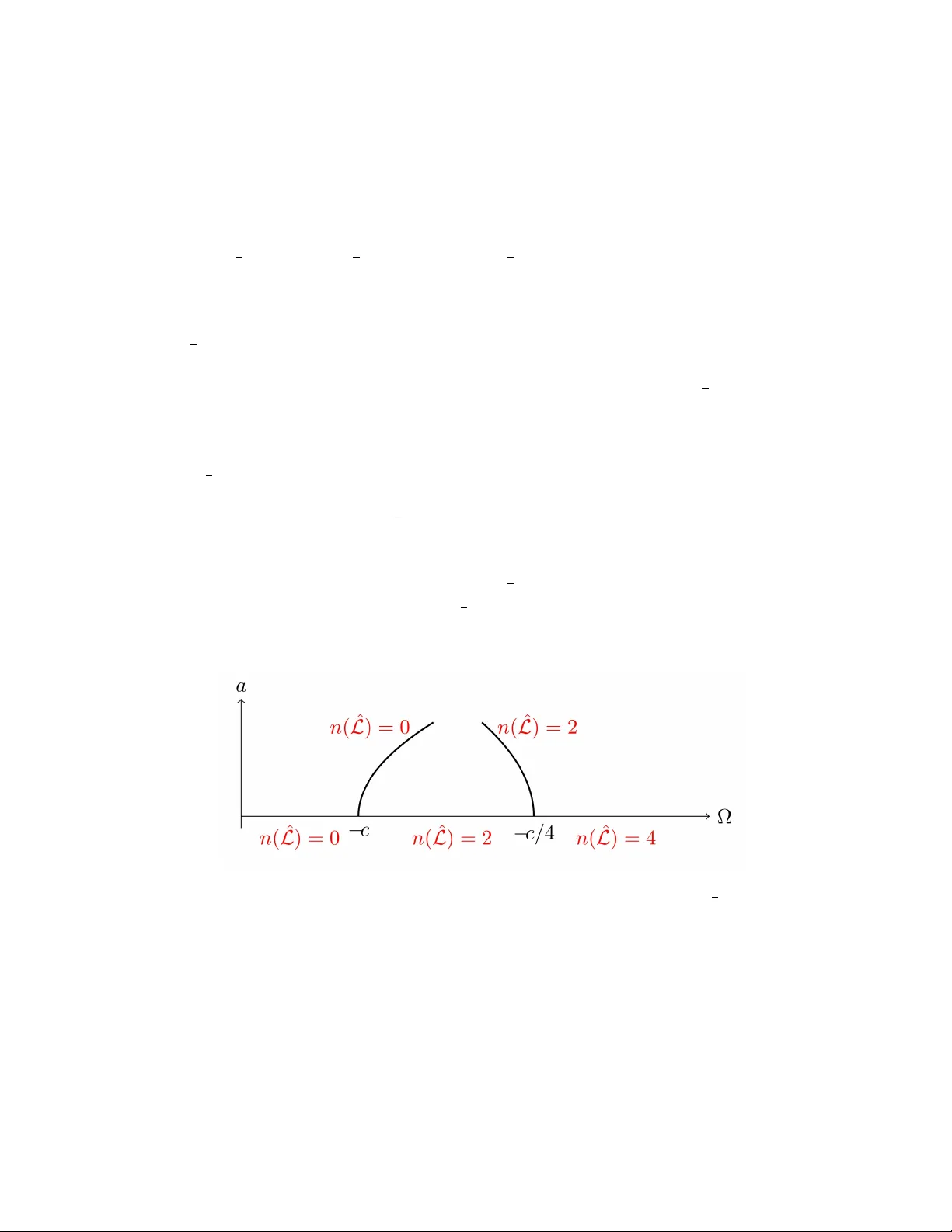
BIFUR CA TIONS OF SOLIT AR Y W A VES IN A COUPLED SYSTEM OF LONG AND SHOR T W A VES JAMES HORNICK AND DMITR Y E. PELINO VSKY Abstract. W e consider families of solitary wa v es in the Kortew eg–de V ries (KdV) equation coupled with the linear Sc hr¨ odinger (LS) equation. This mo del has b een used to describ e interactions b etw een long and short wa v es. T o c haracterize families of solitary w av es, we consider a sequence of lo cal (pitchfork) bifurcations of the uncoupled KdV solitons. The first member of the sequence is the KdV soliton coupled with the ground state of the LS equation, which is prov en to b e the constrained minimizer of energy for fixed mass and momentum. The other members of the sequence are the KdV solitons coupled with the excited states of the LS equation. W e connect the first tw o bifurcations with the exact solutions of the KdV–LS system frequently used in the literature. 1. Intr oduction Coupling b et ween long nonlinear dispersive w a v es and short linear high-frequency w a v e pac k ets can b e mo deled by using the coupled system of the Kortew eg-de V ries (KdV) equation and the linear Sc hr¨ odinger (LS) equation: ( u t + αuu x + β u xxx + γ ( | ψ | 2 ) x = 0 , iψ t + κψ xx + σ uψ = 0 , (1.1) where α, β , γ , κ, σ are nonzero real constan ts, which depend on the small parameter of the original physical problem. The coupled KdV–LS system (1.1) was prop osed to describ e v arious ph ysical mo dels including the resonan t in teraction of capillary-gravit y wa v es [17], in teraction b et w een short surface wa v es and long in ternal wa v es [14], the electron propagation coupled to nonlinear ion-acoustic wa v es in a collisionless plasma [24], and more recen tly , the energy transp ort b y electrons in anharmonic lattices [6]. The KdV–LS system (1.1) was further used for mo deling of the interaction b et w een internal and surface wa v es in a tw o-la y er stratified fluid [7, 8] (see also [26]). Long internal solitons are mo deled by the KdV equation and the short mo dulated surface w av es are mo deled b y the LS equation. The in teraction provides a to ol to detect in ternal wa v es from the fluid surface [7]. F urther extensions of the coupled mo dels b etw een long and short wa v es were constructed recently for the deep water in [16]. Deriv ation of the KdV–LS system (1.1) w as reviewed in [23], where it w as p ointed out that the presence of different scales among the co efficien ts of the mo del mak es the rigorous deriv ation c hallenging. See also the follo w-up work [19] for the study of well-posedness of 1 2 J. HORNICK AND D. E. PELINOVSKY the coupled mo dels. By using the co ordinate transformation x → λ 1 x, t → λ 2 t, u → λ 3 u, ψ → λ 4 ψ with λ 1 = κ β , λ 2 = κ 3 β 2 , λ 3 = αβ κ 2 , λ 4 = p | αγ | β 2 κ 2 , the original coupled system (1.1) can b e transformed to the normalized form: ( u t + uu x + u xxx + s ( | ψ | 2 ) x = 0 , iψ t + ψ xx + k uψ = 0 , (1.2) where k = σ β ακ ∈ R , and s = sgn( αγ ) = ± 1 . If κ = O ( ε − 1 ), σ = O ( ε − 1 ) and γ = O ( ε 2 p ) in terms of the physically relev an t small parameter ε > 0 with some p ∈ (0 , 1), see [7], then k = O (1) is indep endent of ε , so that the normalized form (1.2) is also indep endent of ε . Similarly , the coupled mo del for the capillary–gra vit y w a v es with additional transp ort terms derived in [17] is transformed to the normalized form (1.2) b y using the Galilean transformation. The coupled KdV–LS system (1.2) is Hamiltonian with the follo wing conserv ed quan- tities: Q ( ψ ) = s k Z | ψ | 2 dx, (1.3) P ( u, ψ ) = 1 2 Z  u 2 + is k ( ψ ψ x − ψ ψ x )  dx, (1.4) H ( u, ψ ) = 1 2 Z  ( u x ) 2 − 1 3 u 3 + 2 s k | ψ x | 2 − 2 su | ψ | 2  dx, (1.5) whic h hav e the ph ysical meaning of mass, momentum, and energy , resp ectiv ely . The coupled KdV–LS system (1.2) admits a family of uncoupled KdV solitons, for whic h ψ = 0. Existence of coupled solitary wa v es with ψ  = 0 was studied recently in [3, 5]. Stabilit y of the explicit family of coupled solitary wa ves was shown in [18]. In the case s = − 1 and k < 0, coupled solitary w a v es w ere studied in [1, 2, 4] by using the concentration compactness method, from whic h the existence and orbital stabilit y of a global minimizer of energy H for fixed mass Q and momen tum P follo w. Within the v ariational metho ds, it is difficult to clarify the admissible v alues of the wa ve sp eed and frequency , for which the constrained minimizer of energy is realized, as well as the corresp onding profile ( u, ψ ) of the coupled solitary wa v es. The main purp ose of our work is to clarify the existenc e and stability of families of c ouple d solitary waves by studying their lo c al bifur c ations fr om the family of unc ouple d KdV solitons for s = +1 and k > 0 . This approac h allo ws us to connect the tw o families of coupled solitary w a v es obtained in [3] to the first tw o local (pitchfork) bifurcations in a sequence of bifurcations of the family of the uncoupled KdV solitons. BIFUR CA TIONS OF COUPLED SOLIT AR Y W A VES 3 By using the Ly apuno v–Schmidt reduction, we not only pro ve the existence of families of coupled solitary w a v es within the admissible v alues of the w a v e sp eed and frequency , but also we study the Morse index of the Hessian op erator asso ciated with the v ariational form ulation of the wa v e profile ( u, ψ ) as a constrained minimizer of energy for fixed mass and momentum. As the main outcome of our analysis, w e prov e that the coupled sign-definite solitary w av e is a constrained minimizer of energy and the coupled sign- indefinite solitary wa v es are saddle p oints of the constrained energy . As a part of explicit computations, w e also recov er the stability conclusion for the exact sign-definite solitary w a ves obtained in [18]. It is interesting that our conclusions remain v alid for b oth sup ercritical and subcritical pitc hfork bifurcations of coupled solitary wa v es. Based on n umerical approximations, w e sho w that b oth the sup ercritical and sub critical pitc hfork bifurcations do o ccur for the first t wo bifurcations, dep ending on the parameter k > 0 in the system (1.2) with s = +1. These results agree with the qualitative studies of pitc hfork bifurcations (among the other bifurcations) under the presence of symmetries in the generalized NLS equation [27]. The pap er is organized as follows. Section 2 presents our main results on the existence, bifurcations, and v ariational c haracterization of the solitary wa v es in the coupled KD V– LS system (1.2). Section 3 giv es details of analysis of the uncoupled KdV solitons with precise computations of the Morse index and the sequence of bifurcation p oin ts. Sections 4 and 5 rep ort on the analysis of the first tw o pitchfork bifurcations. The analysis in Sections 3, 4, and 5 pro vides the pro of of the main results. 2. Main resul ts 2.1. Existence of trav eling wa v es. W e consider the trav eling w a v e solutions of the coupled KdV–LS system (1.2) in the form: u ( x, t ) = U ( ξ ) , ψ ( x, t ) = e − iω t Ψ( ξ ) , ξ = x − ct, (2.1) where the profiles U : R → R and Ψ : R → C satisfy the following system of differential equations: ( U ′′′ − cU ′ + U U ′ + s ( | Ψ | 2 ) ′ = 0 , Ψ ′′ − ic Ψ ′ + k U Ψ + ω Ψ = 0 . (2.2) In tegrating the first equation of the system (2.2), we obtain U ′′ − cU + 1 2 U 2 + s | Ψ | 2 = C 1 , (2.3) where C 1 is an in tegration constan t. If U ( ξ ) → 0 and | Ψ( ξ ) | 2 → 0 as | ξ | → ∞ , then C 1 = 0. T o in tegrate the second equation of the system (2.2), w e use the p olar form Ψ = Ae i Θ and obtain ( A ′′ + ( ω + k U ) A + Θ ′ ( c − Θ ′ ) A = 0 , Θ ′′ A + 2Θ ′ A ′ − cA ′ = 0 . (2.4) 4 J. HORNICK AND D. E. PELINOVSKY Multiplying the second equation of the system (2.4) by A and in tegrating, we obtain Θ ′ = C 2 A 2 + c 2 , where C 2 is another in tegration constan t. If A ( ξ ) → 0 as | ξ | → ∞ , then w e ha v e to c ho ose C 2 = 0 to a v oid divergence of Θ ′ ( ξ ) at infinity , whic h yields Θ ′ ( ξ ) = c 2 . Equation (2.3) and the first equation of the system (2.4) are now written as the system of t w o second-order differen tial equations for the profiles U : R → R and A : R → R : ( U ′′ − cU + 1 2 U 2 + sA 2 = 0 , A ′′ + (Ω + k U ) A = 0 , (2.5) where Ω := ω + c 2 4 . The system (2.5) has the first in v ariant: H ( U, A ) = 1 2 ( U ′ ) 2 − c 2 U 2 + 1 6 U 3 + s k ( A ′ ) 2 + sU A 2 + Ω s k A 2 = E , (2.6) where E is constant along solutions of the system (2.5). The first in v ariant (2.6) gives the energy of the degree-tw o Hamiltonian system expressed b y (2.5). If the system admits the second in v ariant, then it is Liouville in tegrable [15]. Analysis of the exact solitary wa v e solutions to the system (2.5) w as dev elop ed in [3] (see also [5]). If A = 0, the system reduces to the scalar equation U ′′ − cU + 1 2 U 2 = 0 , (2.7) whic h is the trav eling w a v e reduction of the integrable KdV equation. Solving (2.7) yields the uncoupled KdV soliton for arbitrary k , U = 3 c sech 2  √ c 2 ξ  , A = 0 , (2.8) where c > 0 is assumed. If k = 1 6 , the system (2.5) is obtained from the tra v eling w av e reduction of the integrable (Melnik o v) system deriv ed in [20] and analyzed in [21, 22]: ( ( u t + uu x + u xxx ) x − 3 u y y + s ( | ψ | 2 ) xx = 0 , − iψ y + ψ xx + 1 6 uψ = 0 . (2.9) Then, u ( x, y , t ) = U ( x − ct ) and ψ ( x, y , t ) = e i Ω y A ( x − ct ) reduces (2.9) to (2.5) with k = 1 6 . Exact solutions for the coupled solitons of the Melniko v system (2.9) were obtained in [22]. F or k = 1 6 , the coupled soliton of the system (2.5) obtained from (2.9) is giv en by ( U = − 12Ω sech 2 ( √ − Ω ξ ) , A = p − 12 s Ω( c + 4Ω) sech( √ − Ω ξ ) , (2.10) where Ω < 0 is assumed. The solution (2.10) is well-defined if s ( c + 4Ω) > 0. If c > 0, this can b e satisfied with tw o options: (a) s = 1: Ω > − c 4 , BIFUR CA TIONS OF COUPLED SOLIT AR Y W A VES 5 (b) s = − 1: Ω < − c 4 . The exact solution (2.10) is widely used in the literature, e.g. [1, 18]. It exists b ecause the system (2.5) is Liouville in tegrable for k = 1 6 . Indeed, by using (3.2.26) and (3.2.27) in [15], w e obtain the second in v arian t of the degree-tw o Hamiltonian system: I ( U, A ) = A ( A ′ )( U ′ ) − U ( A ′ ) 2 + A 2  Ω U + 1 12 U 2 + s 4 A 2  + 3( c + 4Ω)(( A ′ ) 2 + Ω A 2 ) . (2.11) In addition to (2.8) and (2.10), there exists another family of exact solutions of the system (2.5) based on [3]. This additional family is not related to the tw o in tegrable cases. It exists for v arying v alues of the parameter k of the system (2.5): k = − 3Ω c − 2Ω , ( U = 2( c − 2Ω) sech 2 ( √ − Ω ξ ) , A = p 2 s ( c + 4Ω)( c − 2Ω) sech( √ − Ω ξ ) tanh( √ − Ω ξ ) , (2.12) where c > 0 and Ω < 0 are again assumed so that c − 2Ω > 0. The solution (2.12) is w ell-defined if s ( c + 4Ω) > 0, whic h is the same condition as for the solution (2.10) with the same t wo options (a) and (b). The family (2.12) for Ω = − c and s = − 1 corresp onds to k = 1, for whic h the second inv ariant of the system (2.5) can b e obtained by using (3.2.22) in [15]: I ( U, A ) = ( A ′ )( U ′ ) − cAU + s 3 A 3 + 1 2 AU 2 . (2.13) W e did not find the second in v ariant of the system (2.5) for other v alues of Ω and s in the solution (2.12). Remark 1. The exact solutions (2.10) and (2.12) exist for c < 0 if s = − 1 (and c − 2Ω > 0 for the solution (2.12)). However, we do not c onsider the values of c < 0 sinc e we would like to c onne ct the exact solutions (2.10) and (2.12) to the unc ouple d solitons in the form (2.8) by me ans of lo c al bifur c ations. Remark 2. The system (2.5) enjoys the fol lowing r eversibility symmetry: If U ( ξ ) and A ( ξ ) is the solution pr ofile, then so ar e U ( − ξ ) and ± A ( − ξ ) . The solution is invariant under the r eversibility symmetry if U is sp atial ly even and A is either sp atial ly even or o dd. The exact solutions (2.8), (2.10), and (2.12) ar e al l invariant under the r eversibility symmetry. Due to the tr anslational symmetry, the r epr esentations (2.8), (2.10), and (2.12) c an b e tr anslate d fr om the p oint of symmetry at ξ = 0 to any p oint ξ = ξ 0 ∈ R . 2.2. V ariational c haracterization. The profile ( U, Ψ) defined b y the system (2.2) is a critical p oint of the augmen ted energy functional: Λ( U, Ψ) = H ( U, Ψ) + cP ( U, Ψ) − ω Q (Ψ) . (2.14) Indeed, applying v ariational deriv ativ es to (2.14) yields the system ( − U ′′ − 1 2 U 2 − s | Ψ | 2 + cU = 0 , − s k Ψ ′′ − sU Ψ + ics k Ψ ′ − ω s k Ψ = 0 , whic h recov ers (2.2) due to (2.3) with C 1 = 0. 6 J. HORNICK AND D. E. PELINOVSKY By using the representation Ψ( ξ ) = A ( ξ ) e icξ 2 , w e obtain the profile ( U, A ) from the system (2.5). The profile ( U, A ) is a critical point of the action functional Λ( U, Ae icξ 2 ) = H ( U, A ) + cP ( U, 0) − Ω Q ( A ) = 1 2 Z  ( U ′ ) 2 + cU 2 − 1 3 U 3 + 2 s k ( A ′ ) 2 − 2 sU A 2 − 2Ω s k A 2  dξ , (2.15) with Ω = ω + c 2 4 . Indeed, the representation Ψ( ξ ) = A ( ξ ) e icξ 2 transforms Λ( U, Ψ) in (2.14) to the form (2.15), v ariational deriv ativ es of whic h generate the system (2.5). The following theorem gives the main result of this w ork. Theorem 1. Assume c > 0 , Ω < 0 , and s = sgn( k ) . If s = − 1 or if s = 1 and Ω < Ω c with Ω c = − c 16  √ 1 + 48 k − 1  2 , (2.16) then the unc ouple d soliton (2.8) is a lo c al minimizer of the c onstr aine d ener gy H for fixe d momentum P de gener ate only by the tr anslational symmetry. If s = 1 and Ω ∈ (Ω c , 0) , then the unc ouple d soliton (2.8) is a sadd le p oint of the c onstr aine d ener gy. F urthermor e, for k > J ( J − 1) 12 with J ∈ N , ther e exist a se quenc e { Ω ( j ) c } J j =1 of pitchfork bifur c ations (either sup er-critic al or sub-critic al) with Ω ( j ) c = − c 16  √ 1 + 48 k − 2 j + 1  2 , 1 ≤ j ≤ J, (2.17) such that new families bifur c ate fr om the family of unc ouple d solitons. The family with j = 1 is a lo c al minimizer of the c onstr aine d ener gy H for fixe d momentum P and mass Q de gener ate only by the tr anslational and r otational symmetries, wher e as the families with j = 2 , . . . , J ar e sadd le p oints of the c onstr aine d ener gy. Remark 3. We use s = sgn( k ) to ensur e that the se c ond variation of the action functional (2.15) at the family of the solitary waves with the pr ofile ( U, A ) b e b ounde d fr om b elow (but not fr om the ab ove). Remark 4. In the c ase of the lo c al minimizers of the c onstr aine d ener gy, the orbital stability of either the unc ouple d soliton (2.8) or the c ouple d solitary wave for p erturb ations ( w , z ) in H 1 ( R , R ) × H 1 ( R , C ) fol lows fr om a gener al ar gument in The or em 2.8 in [11] . However, for the c ase of the sadd le p oints of the c onstr aine d ener gy, the orbital instability do es not fol low imme diately unless the sp e ctr al instability c an b e pr oven, se e The or em 2.4 in [11] . We do not have the sp e ctr al instability of the unc ouple d soliton (2.8) sinc e the KdV e quation is quadr atic al ly c ouple d to the solution of the line ar Schr¨ odinger e quation in the KdV–LS system (1.2). Henc e, we ar e not able to c onclude on the orbital instability of the unc ouple d soliton (2.8) if s = 1 and Ω ∈ (Ω c , 0) . 2.3. Sc hematic illustration and the road map. Figure 1 presen ts the bifurcation diagram for the three families of solitary wa v e solutions of the system (2.5) with s = 1, k = 1 2 , and a fixed v alue of c > 0. The bifurcation parameter is Ω < 0. The family of uncoupled KdV solitons in the form (2.8) corresp onds to the horizontal line and defines BIFUR CA TIONS OF COUPLED SOLIT AR Y W A VES 7 the primary br anch for pitc hfork bifurcations. In Proposition 1, we sho w that the Morse index n ( b L ) (the num b er of negative eigen v alues of the Hessian op erator constrained b y t w o symmetries of the KdV–LS system) for the primary branch is 0 for Ω < − c , 2 for − c < Ω < − c 4 , and 4 for − c 4 < Ω < 0 (if k = 1 2 ). F or Ω < − c , the family of uncoupled KdV solitons is a lo cal minimizer of the constrained energy H for fixed momentum P , hence it is orbitally stable in the time evolution of the KdV–LS system (1.2). Bifurcations of new se c ondary families of coupled solitary w a v es o ccur at Ω = − c and Ω = − c 4 when the n ullit y index (the multiplicit y of the zero eigenv alue of the Hessian op erator) exceeds the num ber of symmetries. In Prop osition 2 and Figure 2, we show that the first bifurcation is a supercritical pitchfork bifurcation (if k = 1 2 ). F urthermore, in Prop ositions 3 and 4, w e show that the Morse index of the bifurcating family is 0 so that it is a lo cal minimizer of the constrained energy H for fixed momentum P and mass Q . The exact solution (2.10) giv es a global con tinuation of this bifurcation (but in the case k = 1 6 ). Finally , in Prop osition 5 and Figure 4, w e show that the second bifurcation is a sub crit- ical pitchfork bifurcation (if k = 1 2 ). F urthermore, in Prop ositions 6 and 7, w e show that the Morse index of the bifurcating family is 2 so that it is a saddle p oint of the constrained energy H for fixed momentum P and mass Q . The exact solution (2.12) bifurcates from the primary branc h for this exact v alue of k = 1 2 . How ev er, it is globally extended in the form (2.12) for different v alues of k in  0 , 1 2  that dep end on the bifurcation parameter Ω, see Figure 3. Figure 1. Schematic bifurcation diagram for s = 1 and k = 1 2 , which sho ws how the families of coupled solitary w a v es generalizing (2.10) and (2.12) are connected with the family (2.8) of the uncoupled KdV solitons. b L denotes the Hessian op erator constrained b y tw o symmetries of the KdV– LS system (1.2) and n ( b L ) is its Morse index. Remark 5. A c c or ding to the r eversibility symmetry in R emark 2, we obtain se c ondary br anches in subsp ac es of functions with even and o dd p arities in the Sob olev sp ac e H 2 ( R ) . We denote these subsp ac es by H 2 even ( R ) and H 2 odd ( R ) , r esp e ctively. 8 J. HORNICK AND D. E. PELINOVSKY 3. St ability and bifurca tions of the uncoupled KdV solitons 3.1. Hessian op erator for the solitary w a v es. The v ariational form ulation of the solitary wa ves with the profile ( U, A ) by using the action functional (2.15) relates the system of differen tial equations (2.5) with the three conserved quan tities of the KdV– LS system (1.2) giv en b y (1.3), (1.4), and (1.5). W e use this construction to define the Hessian op erator for the solitary wa v es. The Hessian op erator plays the central role in the analysis of stability and bifurcations of the solitary w a v es. Lemma 1. L et ( U, A ) ∈ H 1 ( R ) × H 1 ( R ) b e a critic al p oint of the action functional (2.15). The c orr esp onding Hessian is expr esse d by the line ar op er ator L : ( H 2 ( R )) 3 ⊂ ( L 2 ( R )) 3 → ( L 2 ( R )) 3 given by L = −   ∂ 2 ξ + U − c 2 sA 0 2 sA 2 s k  ∂ 2 ξ + k U + Ω  0 0 0 2 s k  ∂ 2 ξ + k U + Ω    . (3.1) Pr o of. Adding a p erturbation ( w , z ) to the profile ( U, Ψ) in the augmen ted energy func- tional (2.14) and using the tra v eling w a v e co ordinate ξ = x − ct , w e obtain the following expansion: Λ( U + w , Ψ + z ) = Z  1 2 ( U ′ + w ′ ) 2 − 1 6 ( U + w ) 3 + s k | Ψ ′ + z ′ | 2 − s ( U + w ) | Ψ + z | 2  dξ + c Z  1 2 ( U + w ) 2 + is 2 k [(Ψ + ¯ z )(Ψ ′ + z ′ ) − (Ψ + z )(Ψ ′ + z ′ )]  dξ − ω s k Z | Ψ + z | 2 dξ . Since ( U, Ψ) is a critical point of Λ( U, Ψ), w e get the expansion Λ( U + w , Ψ + z ) = Λ( U, Ψ) + 1 2 Q 2 ( w , z ) + 1 6 Q 3 ( w , z ) , where Q 2 and Q 3 are quadratic and cubic terms in ( w , z ). T o compute the Hessian op erator, we only collect the quadratic terms in Q 2 ( w , z ) = Z  ( w ′ ) 2 − U w 2 + 2 s k | z ′ | 2 − 2 sU | z | 2 − 2 sw (Ψ z + Ψ z )  dξ + c Z  w 2 + is k ( ¯ z z ′ − z z ′ )  dξ − 2 ω s k Z | z | 2 dξ . By using the v ariables Ψ = Ae icξ 2 , z = ( z 1 + iz 2 ) e icξ 2 , (3.2) BIFUR CA TIONS OF COUPLED SOLIT AR Y W A VES 9 with real A and ( z 1 , z 2 ), we rewrite Q 2 ( w , z ) in the form Q 2 ( w , z ) = Z  ( w ′ ) 2 − U w 2 + 2 s k [( z ′ 1 ) 2 + ( z ′ 2 ) 2 ] − 2 sU ( z 2 1 + z 2 2 ) − 4 sw Az 1  dξ + c Z w 2 dξ − 2Ω s k Z ( z 2 1 + z 2 2 ) dξ , where Ω = ω + c 2 4 . Representing Q 2 ( w , z ) as a quadratic form for L acting on ( w , z 1 , z 2 ) in ( L 2 ( R )) 3 yields the Hessian op erator L in the form (3.1). □ It follows from (3.1) that L is blo ck-diagonalized in to a 2 × 2 matrix Sc hr¨ odinger op erator L J : ( H 2 ( R )) 2 ⊂ ( L 2 ( R )) 2 → ( L 2 ( R )) 2 giv en by L J =  L 1 − 2 sA − 2 sA L 2  with  L 1 = − ∂ 2 ξ + c − U, L 2 = 2 s k  − ∂ 2 ξ − Ω − k U  , (3.3) and a scalar Sc hr¨ odinger op erator L 2 : H 2 ( R ) ⊂ L 2 ( R ) → L 2 ( R ). Since U and A decays to zero at infinit y exponentially fast and we hav e assumed that c > 0 and Ω < 0, W eyl’s theorem implies that the con tin uous sp ectrum of L is a union of the con tin uous sp ectra of L 1 and L 2 , whic h are giv en b y [ c, ∞ ) and 2 s k [ | Ω | , ∞ ), respectively . The con tin uous sp ectrum of L is strictly p ositive if and only if s = sgn( k ) , whic h is assumed from no w on, see Theorem 1 and Remark 3. The main task of the stability analysis by using the Lyapuno v theory is to compute the Morse index (the n um b er and m ultiplicit y of negativ e eigen v alues) and the degeneracy index (multiplicit y of the zero eigen v alue) of the Hessian operator L . T o achiev e the task, w e recall the following w ell-kno wn result, see [10]. Lemma 2. L et T : H 2 ( R ) ⊂ L 2 ( T ) → L 2 ( R ) b e the sc alar Schr¨ odinger op er ator given by T = − ∂ 2 x − γ sec h 2 ( x ) , γ > 0 . The c ontinuous sp e ctrum of T is σ c ( T ) = [0 , ∞ ) , wher e as the p oint sp e ctrum of T dep ends on γ and c onsists of simple eigenvalues: σ p ( T ) = ( −  1 2 p 1 + 4 γ − n − 1 2  2 , n = 0 , 1 , 2 , . . . , N ) \{ 0 } , (3.4) wher e N = ⌊ 1 2 ( √ 1 + 4 γ − 1) ⌋ with ⌊ a ⌋ denoting the flo or of a p ositive numb er a . Remark 6. If ⌊ 1 2 ( √ 1 + 4 γ − 1) ⌋ = 1 2 ( √ 1 + 4 γ − 1) , then 0 is the r esonanc e of the Schr¨ odinger op er ator T at the end p oint of σ c ( T ) = [0 , ∞ ) . It is exclude d fr om σ p ( T ) in (3.4), which then c onsists of N ne gative eigenvalues. If ⌊ 1 2 ( √ 1 + 4 γ − 1) ⌋ < 1 2 ( √ 1 + 4 γ − 1) , then σ p ( T ) in (3.4) c onsists of ( N + 1) ne gative eigenvalues. 10 J. HORNICK AND D. E. PELINOVSKY 3.2. Characterization of the uncoupled KdV solitons. Lemmas 1 and 2 give the necessary ingredien ts to study the v ariational c haracterization of the uncoupled KdV soli- ton with the profile ( U, 0), where U is giv en by (2.8). Since A = 0 for the uncoupled KdV soliton (2.8), the mass conserv ation Q pla ys no role in the v ariational c haracterization. Prop osition 1. Assume c > 0 , Ω < 0 , and s = sgn( k ) . If s = − 1 or if s = 1 and Ω < Ω c with Ω c = − c 16  √ 1 + 48 k − 1  2 , (3.5) then the unc ouple d KdV soliton with the pr ofile (2.8) is a lo c al minimizer of the c onstr aine d ener gy H for fixe d momentum P de gener ate only by the tr anslational symmetry. If s = 1 and Ω ∈ (Ω c , 0) , then the unc ouple d KdV soliton is a sadd le p oint of the c onstr aine d ener gy. Pr o of. F or the uncoupled KdV soliton with the profile (2.8), the Hessian op erator (3.1) is diagonal with ( L 1 , L 2 , L 2 ), where L 1 and L 2 are defined in (3.3). Putting y = √ c 2 ξ , w e con v ert L 1 and L 2 to the form used in Lemma 2: ( L 1 = c 4  − ∂ 2 y + 4 − 12sech 2 ( y )  , L 2 = c 2 | k |  − ∂ 2 y + 4 | Ω | c − 12 k sec h 2 ( y )  . (3.6) By Lemma 2, the normalized op erator T 1 = − ∂ 2 y + 4 − 12sech 2 ( y ) has three eigen v alues − 5 , 0 , 3 isolated from the con tin uous sp ectrum on [4 , ∞ ). Therefore, L 1 has a simple negativ e eigenv alue and a simple zero eigenv alue with the eigenfunction spanned by U ′ due to the translational symmetry . If s = sgn( k ) = − 1, the normalized op erator T 2 = − ∂ 2 y + 4 | Ω | c + 12 | k | sec h 2 ( y ) has no isolated eigenv alues from the con tin uous sp ectrum on h 4 | Ω | c , ∞  . If s = sgn( k ) = +1, the normalized op erator T 2 = − ∂ 2 y + 4 | Ω | c − 12 k sec h 2 ( y ) has the smallest eigen v alue at 4 | Ω | c − 1 4  √ 1 + 48 k − 1  2 . F or Ω < Ω c , where Ω c is giv en b y (3.5), it is strictly p ositive, whereas for Ω ∈ (Ω c , 0), it is strictly negativ e. W e conclude that for s = − 1 or if s = 1 and Ω < Ω c , the Morse index of the uncoupled KdV soliton with the profile ( U, 0) in (2.8) is exactly 1 and the degeneracy index is exactly 1. By Theorem 2.7 in [11], ( U, 0) is a lo cal constrained minimizer of energy H sub ject to fixed momentum P degenerate only b y the translational symmetry if and only if the slop e condition is satisfied: d dc P ( U, 0) > 0 . This is true since P ( U, 0) = 9 c 2 2 Z R sec h 4  √ cξ 2  dξ = 12 c 3 2 (3.7) BIFUR CA TIONS OF COUPLED SOLIT AR Y W A VES 11 so that d dc P ( U, 0) > 0 and the statement is prov en. If s = 1 and Ω ∈ (Ω c , 0), the Morse index of the uncoupled KdV soliton with the profile ( U, 0) in (2.8) is at least 3. By Theorem 2.7 in [11], ( U, 0) is a saddle p oint of the constrained energy . □ Remark 7. Op er ator L 2 in (3.6) admits zer o eigenvalues at { Ω ( n ) c } J j =1 , wher e Ω ( j ) c is given by (2.17) with Ω (1) c ≡ Ω c and J define d by the lar gest inte ger such that k > J ( J − 1) 12 . At Ω = Ω ( j ) , the primary br anch of the unc ouple d KdV solitons under go es a lo c al bifur c ation and a new se c ondary br anch of the c ouple d solitary waves app e ars. In Se ction 4 and 5, we study the first two bifur c ations, for which the new se c ondary br anches include the exact solutions (2.10) and (2.12), r esp e ctively. 4. Bifur ca tion of the coupled solit ar y w a ve a t Ω (1) c ≡ Ω c 4.1. The bifurcating branch of coupled solitary w a v es. By Prop osition 1, the first bifurcation along the family of the uncoupled KdV solitons o ccurs at Ω = Ω c , for which the first p ositiv e eigen v alue of the Sc hr¨ odinger op erator L 2 : H 2 ( R ) ⊂ L 2 ( R ) → L 2 ( R ) for Ω < Ω c passes through zero and b ecomes negative for Ω > Ω c . The first eigen v alue of L 2 corresp onds to the following eigenfunction: g ( ξ ) = sech p  √ c 2 ξ  , p = √ 1 + 48 k − 1 2 . (4.1) Note that Ω c = − c 4 and p = 1 if k = 1 6 , for whic h the profiles U in (2.8) and g in (4.1) coincide with the profile ( U, A ) of the coupled solitary wa v e giv en by (2.10) for Ω = Ω c . Since s = sgn( k ) = +1, the solution family (2.10) exists for Ω ∈ (Ω c , 0), for which the solution family (2.8) is a saddle p oin t of the constrained energy b y Proposition 1. The following result shows that the in tersection of the branc h of coupled solitary wa ves (2.10) with the branc h of uncoupled KdV solitons (2.8) at Ω = Ω c is not a coincidence but the outcome of a local pitc hfork bifurcation whic h is v alid for ev ery k > 0 near Ω = Ω c . Prop osition 2. Assume c > 0 , Ω < 0 , and s = sgn( k ) = 1 . L et U 0 b e given by (2.8) and g b e given by (4.1). Assume that ⟨ g 2 , L − 1 1 g 2 ⟩  = 0 , wher e L 1 is define d in (3.6). F or every Ω ne ar Ω c such that sgn(Ω − Ω c ) = − sgn( ⟨ g 2 , L − 1 1 g 2 ⟩ ) , ther e exists a unique family of solutions with the pr ofile ( U, A ) ∈ H 2 even ( R ) × H 2 even ( R ) satisfying ∥ U − U 0 ∥ H 2 ≤ C | Ω − Ω c | , ∥ A ∥ ≤ C p | Ω − Ω c | , for some Ω -indep endent c onstant C > 0 . Pr o of. W e represent the system of equations (2.5) as the root finding problem for the v ector field F ( U, A, Ω) : H 2 ( R ) × H 2 ( R ) × R → L 2 ( R ) × L 2 ( R ) , (4.2) with F ( U, A, Ω) =  − U ′′ + cU − 1 2 U 2 − sA 2 2 s k ( − A ′′ − (Ω + k U ) A )  , 12 J. HORNICK AND D. E. PELINOVSKY where c > 0 and k > 0 are fixed and s = sgn( k ) = 1. The Jacobian of F at ( U, A ) is giv en b y the matrix Schr¨ odinger operator L J : ( H 2 ( R ) 2 ⊂ ( L 2 ( R )) 2 → ( L 2 ( R )) 2 in (3.3). Ev aluating L J at ( U, A, Ω) = ( U 0 , 0 , Ω c ) with U 0 giv en by (2.8) and using p erturbation ( w , z , δ Ω) to ( U 0 , 0 , Ω c ) yields the expansion F ( U 0 + w , z , Ω c + δ Ω) = F ( U 0 , 0 , Ω c ) | {z } =0 +  L 1 0 0 L 2   w z  +  − 1 2 w 2 − sz 2 − 2 sw z − 2 s k δ Ω z  , (4.3) where the explicit form of the Sc hr¨ odinger op erators L 1 and L 2 is given in (3.6) for Ω = Ω c . The ro ot-finding problem for F can be rewritten in the form  L 1 0 0 L 2   w z  =  1 2 w 2 + sz 2 2 sw z + 2 s k δ Ω z  . (4.4) W e recall that ker L 1 = span( U ′ 0 ) and k er L 2 = span( g ), where U ′ 0 is o dd and g is even in ξ . T o eliminate the translational symmetry , we consider the implicit equation (4.4) on the subspace of even functions ( w , z ) ∈ H 2 even ( R ) × H 2 even ( R ), for which L 1 is inv ertible with a b ounded in v erse. The implicit equation (4.4) is closed on this subspace, thanks to the rev ersibilit y symmetry of the system (2.5), see Remark 2. Therefore, w e use the orthogonal decomp osition  w z  = a  0 g  +  w 1 z 1  , suc h that ⟨ g , z 1 ⟩ = 0 , (4.5) with a ∈ R b eing a (small) parameter defined b y the orthogonality constrain t with the standard inner pro duct ⟨· , ·⟩ in L 2 ( R ). The implicit equation (4.4) is rewritten in the form:  L 1 0 0 L 2   w 1 z 1  =  1 2 w 2 1 + s ( ag + z 1 ) 2 2 sw 1 ( ag + z 1 ) + 2 s k δ Ω( ag + z 1 )  . (4.6) Orthogonalit y of the second equation of system (4.6) to ker L 2 = span( g ) yields the solv- abilit y condition δ Ω a ∥ g ∥ 2 L 2 + k ⟨ g , w 1 ( ag + z 1 ) ⟩ = 0 . (4.7) Under the constrain t (4.7), L 2 is in v ertible with a b ounded in v erse on a subspace of L 2 ( R ) orthogonal to k er L 2 = span( g ). This allows us to rewrite the implicit equation (4.6) in the final form:  w 1 z 1  =  L − 1 1 0 0 L − 1 2  1 2 w 2 1 + s ( ag + z 1 ) 2 2 sw 1 ( ag + z 1 ) − 2 s ( ag + z 1 ) ⟨ g ,w 1 ( ag + z 1 ) ⟩ a ∥ g ∥ 2 L 2 ! . (4.8) By the implicit function theorem, there exists a unique solution ( w 1 , z 1 ) ∈ H 2 even ( R ) × H 2 even ( R ) to (4.8) such that ⟨ g , z 1 ⟩ = 0 for every (sufficien tly small) a ∈ R and the mapping a 7→ ( w 1 , z 1 ) is C ∞ . Let us denote the unique solution as ( w 1 ( a ) , z 1 ( a )). It follo ws from the principal terms of the system (4.8) that the mapping satisfies ∥ w 1 ( a ) ∥ H 2 ≤ C a 2 , ∥ z 1 ( a ) ∥ H 2 ≤ C | a | 3 , (4.9) BIFUR CA TIONS OF COUPLED SOLIT AR Y W A VES 13 for some C > 0 uniformly for small a ∈ R . F or precise computations, w e need the follo wing transformation w 1 ( a ) = a 2 w 2 + w 2 ( a ) , ∥ w 2 ( a ) ∥ H 2 ≤ C a 4 , (4.10) where the a -indep enden t function w 2 ∈ H 2 even ( R ) is giv en by w 2 = sL − 1 1 g 2 . Substituting ( w 1 ( a ) , z 1 ( a )) satisfying (4.9) and (4.10) in to (4.7), w e obtain δ Ω = − ka 2 ⟨ g 2 , L − 1 1 g 2 ⟩ ∥ g ∥ 2 L 2 + O ( a 4 ) , (4.11) whic h sho ws that sgn( δ Ω) = − sgn( ⟨ g 2 , L − 1 1 g 2 ⟩ ) since k > 0. This completes the pro of. □ 4.2. Characterization of the bifurcating branch. W e first compute the Morse index and the n ullit y index of the bifurcating branc h in Prop osition 2. Prop osition 3. L et ( U, A ) b e the pr ofile of the bifur c ating br anch for Ω ne ar Ω c given by Pr op osition 2. Its Morse index is e qual to 1 if ⟨ g 2 , L − 1 1 g 2 ⟩ < 0 and to 2 if ⟨ g 2 , L − 1 1 g 2 ⟩ > 0 , wher e as the nul lity index is e qual to 2 in b oth c ases. Pr o of. W e use the construction of Prop osition 2 with the profile U = U 0 + w 1 ( a ) and A = ag + z 1 ( a ) , (4.12) where ( w 1 ( a ) , z 1 ( a )) ∈ H 2 even ( R ) × H 2 even ( R ) satisfy the bounds (4.9). The parameter a > 0 parameterize the bifurcating branch, in particular, we hav e Ω = Ω c + δ Ω( a ), where δ Ω( a ) is given b y the expansion (4.11) with sgn( δ Ω) = − sgn( ⟨ g 2 , L − 1 1 g 2 ⟩ ). The Hessian blo ck L J defined by (3.3) can b e expanded b y using (4.12) as follo ws: L J =  L 1 − w 1 ( a ) − 2 s ( ag + z 1 ( a )) − 2 s ( ag + z 1 ( a )) L 2 − 2 s w 1 ( a ) − 2 s k δ Ω( a )  =  L 1 0 0 L 2  + a  0 − 2 sg − 2 sg 0  + a 2 − sL − 1 1 g 2 0 0 − 2 L − 1 1 g 2 + 2 ⟨ g 2 ,L − 1 1 g 2 ⟩ ∥ g ∥ 2 L 2 ! + O ( a 3 ) = L (0) J + aL (1) J + a 2 L (2) J + O ( a 3 ) , where we hav e used the leading-order terms for w 1 ( a ) and δ Ω( a ) from (4.10) and (4.11). W e are now lo oking at the eigen v alues and eigen v ectors of the eigen v alue equation L J v = λv . Since 0 is a double eigenv alue of L (0) J , we are lo oking for the splitting of the zero eigen v alue b y using the p erturbation theory . W e write v = v (0) + av (1) + a 2 v (2) + O ( a 3 ) , λ = aλ (1) + a 2 λ (2) + O ( a 3 ) , where v (0) = c 1  U ′ 0 0  + c 2  0 g  for some ( c 1 , c 2 ) ∈ R 2 . A t the order of O ( a ), w e obtain L (0) v (1) + L (1) v (0) = λ (1) v (0) . 14 J. HORNICK AND D. E. PELINOVSKY W riting in the comp onen t form, w e obtain v 1 =  f 1 g 1  :  L 1 f 1 − 2 sg ( c 2 g ) = λ (1) ( c 1 U ′ 0 ) , L 2 g 1 − 2 sg ( c 1 U ′ 0 ) = λ (1) ( c 2 g ) . Since ev en g 2 is orthogonal to U ′ 0 and o dd g U ′ 0 is orthogonal to even g , w e obtain by F redholm’s theory for linear inhomogeneous equations that λ (1) = 0. This yields the exact solution in the form f 1 = 2 sc 2 L − 1 1 g 2 , g 1 = 2 sc 1 L − 1 2 g U ′ 0 , where L − 1 1 is uniquely defined in the space of ev en functions and L − 1 2 is uniquely defined in the space of odd functions. Differentiating of ( − ∂ 2 ξ − Ω c − k U 0 ) g = 0 in ξ yields L 2 g ′ = 2 sU ′ 0 g , whic h ensures that g 1 = c 1 g ′ . A t the order of O ( a 2 ), we obtain L (0) v (2) + L (1) v (1) + L (2) v (0) = λ (2) v (0) . W riting in the comp onen t form, w e obtain v 2 =  f 2 g 2  : ( L 1 f 2 − 2 sg g 1 − s ( L − 1 1 g 2 )( c 1 U ′ 0 ) = λ (2) ( c 1 U ′ 0 ) , L 2 g 2 − 2 sg f 1 +  − 2 L − 1 1 g 2 + 2 ⟨ g 2 ,L − 1 1 g 2 ⟩ ∥ g ∥ 2 L 2  ( c 2 g ) = λ (2) ( c 2 g ) . T aking the inner pro duct of the first equation with U ′ 0 ∈ Ker( L 1 ) and also taking the inner pro duct of the second equation with g ∈ Ker( L 2 ), we get the linear system for ( c 1 , c 2 ) ∈ R 2 : − 4 c 1 ⟨ g U ′ 0 , L − 1 2 g U ′ 0 ⟩ − sc 1 ⟨ ( U ′ 0 ) 2 , L − 1 1 g 2 ⟩ = λ (2) c 1 ∥ U ′ 0 ∥ 2 L 2 , − 4 c 2 ⟨ g 2 , L − 1 1 g 2 ⟩ = λ (2) c 2 ∥ g ∥ 2 L 2 where we ha v e used the explicit expressions for f 1 , g 1 . Since the linear system is diagonal, w e get t w o different solutions related to the subspaces ( c 1 , c 2 ) = (1 , 0) and ( c 1 , c 2 ) = (0 , 1). F or the subspace ( c 1 , c 2 ) = (1 , 0), we pro ve that 4 ⟨ g U ′ 0 , L − 1 2 g U ′ 0 ⟩ + s ⟨ ( U ′ 0 ) 2 , L − 1 1 g 2 ⟩ = 0 , (4.13) whic h yields λ (2) = 0. This is consistent with the fact that the zero eigenv alue λ = 0 is preserv ed along the solution branc h with the profile ( U , A ) b y the translational symmetry . T o v erify (4.13), w e derive from U ′′ 0 = cU 0 − 1 2 U 2 0 , ( U ′ 0 ) 2 = cU 2 0 − 1 3 U 3 0 , that L 1 U 0 = − U ′′ 0 + cU 0 − U 2 0 = − 1 2 U 2 0 , L 1 U 2 0 = − 2 U 0 U ′′ 0 − 2( U ′ 0 ) 2 + cU 2 0 − U 3 0 = − 3 cU 2 0 + 2 3 U 3 0 . BIFUR CA TIONS OF COUPLED SOLIT AR Y W A VES 15 Hence we obtain ⟨ ( U ′ 0 ) 2 , L − 1 1 g 2 ⟩ = c ⟨ U 2 0 , L − 1 1 g 2 ⟩ − 1 3 ⟨ U 3 0 , L − 1 1 g 2 ⟩ = c ⟨ L − 1 1 U 2 0 , g 2 ⟩ − 1 3 ⟨ L − 1 1 U 3 0 , g 2 ⟩ = − c 2 ⟨ L − 1 1 U 2 0 , g 2 ⟩ − 1 2 ⟨ U 2 0 , g 2 ⟩ = c ⟨ U 0 , g 2 ⟩ − 1 2 ⟨ U 2 0 , g 2 ⟩ . On the other hand, since L − 1 2 g U ′ 0 = s 2 g ′ , we also obtain 4 ⟨ g U ′ 0 , L − 1 2 g U ′ 0 ⟩ = 2 s ⟨ g U ′ 0 , g ′ ⟩ = − s ⟨ U ′′ 0 , g 2 ⟩ = − cs ⟨ U 0 , g 2 ⟩ + s 2 ⟨ U 2 0 , g 2 ⟩ . Substituting these computations into the left-hand side of (4.13), w e obtain the zero result. F or the subspace ( c 1 , c 2 ) = (0 , 1), we get λ (2) = − 4 ⟨ g 2 , L − 1 1 g 2 ⟩ ∥ g ∥ 2 L 2 whic h shows that λ = a 2 λ (2) + O ( a 3 ) > 0 if ⟨ g 2 , L − 1 1 g 2 ⟩ < 0 and λ = a 2 λ (2) + O ( a 3 ) < 0 if ⟨ g 2 , L − 1 1 g 2 ⟩ > 0. Since L (0) J has only one negative eigen v alue at U = U 0 , the splitting of the double zero eigenv alue of L (0) J is clarified abov e, and the other eigenv alues of L (0) J are strictly p ositiv e, the cont inuit y of eigenv alues in a implies that the Morse index of L J is 1 if ⟨ g 2 , L − 1 1 g 2 ⟩ < 0 and 2 if ⟨ g 2 , L − 1 1 g 2 ⟩ > 0 for small a  = 0. Referring back to the Hessian op erator L given b y (3.1), it follows that the operator L 2 = − 2 s k ( ∂ 2 ξ + k U + Ω) admits a simple zero eigen v alue due to the rotational symmetry with L 2 A = 0. The rest of L 2 at U = U 0 and Ω = Ω c is strictly p ositiv e, hence the Morse index of L 2 is 0 for small a . This yields the claim on the Morse index of L . On the other hand, L has a double zero eigen v alue asso ciated with the translational and rotational symmetries, and the splitting of the double zero eigen v alue of L (0) J clarified ab o v e sho ws that the kernel of L is exactly double for small a . This yields the claim ab out the n ullity index of L . □ W e next clarify the constrained minimization prop erties of the bifurcating branc h b y using information ab out the Morse and n ullit y indices from Prop osition 3. Prop osition 4. L et ( U, A ) b e the pr ofile of the bifur c ating br anch for Ω ne ar Ω c given by Pr op osition 2. If either ⟨ g 2 , L − 1 1 g 2 ⟩ < 0 or ⟨ g 2 , L − 1 1 g 2 ⟩ > 0 , the bifur c ating br anch is a lo c al minimizer of the c onstr aine d ener gy H for fixe d momentum P and mass Q de gener ate only by the tr anslational and r otational symmetries. 16 J. HORNICK AND D. E. PELINOVSKY Pr o of. W e use again the decomp osition (4.12) with Ω = Ω c + δ Ω( a ), where ( w 1 ( a ) , z 1 ( a )) ∈ H 2 even ( R ) × H 2 even ( R ) satisfy the b ounds (4.9) and δ Ω( a ) is given b y the expansion (4.11). Hence, we compute  P ( U, 0) = 1 2 ∥ U 0 ∥ 2 L 2 + ⟨ U 0 , w 1 ( a ) ⟩ + 1 2 ∥ w 1 ( a ) ∥ 2 L 2 , Q ( A ) = s k  a 2 ∥ g ∥ 2 L 2 + 2 a ⟨ g , z 1 ( a ) ⟩ + ∥ z 1 ( a ) ∥ 2 L 2  . (4.14) W e recall the action functional (2.15) rewritten as Λ( U, Ψ) = H ( U, A ) + cP ( U, 0) + | Ω | Q ( A ) T o incorporate the constrain ts of fixed momen tum P and mass Q in the minimization of energy H , w e consider the Hessian op erator L on the constrained subspace of ( L 2 ( R )) 3 for the p erturbation ( w , z 1 , z 2 ) satisfying the following t w o constraints: ⟨ U, w ⟩ = 0 and ⟨ A, z 1 ⟩ = 0 , where w is the perturbation to U and z 1 + iz 2 is the p erturbation to A according to (3.2). The constrained Hessian op erator is denoted by ˆ L . By Theorem 3.2 in [11], the Morse index n ( ˆ L ) and the nullit y index z ( ˆ L ) are computed as  n ( ˆ L ) = n ( L ) − p 0 − z 0 , z ( ˆ L ) = z ( L ) + z 0 , (4.15) where p 0 and z 0 are the n um b er of p ositive and zero eigen v alues of the matrix D giv en by D = ∂ P ( U, 0) ∂ c ∂ P ( U, 0) ∂ | Ω | ∂ Q ( A ) ∂ c ∂ Q ( A ) ∂ | Ω | ! F or the bifurcating branch, we use parameters c and a 2 with the dep endence Ω = Ω c + δ Ω( a ) expressed in even p ow ers of the small amplitude a . Hence, w e in tro duce the function ( c, Ω) → a 2 b y solving the implicit equation Ω = Ω c + δ Ω( a ) for Ω close to Ω c . By using the chain rule, we obtain D =  ∂ P ( U, 0) ∂ c + ∂ P ( U, 0) ∂ a 2 ∂ a 2 ∂ c − ∂ P ( U, 0) ∂ a 2 ∂ a 2 ∂ Ω ∂ Q ( A ) ∂ c + ∂ Q ( A ) ∂ a 2 ∂ a 2 ∂ c − ∂ Q ( A ) ∂ a 2 ∂ a 2 ∂ Ω ,  It follows from (4.11) that ∂ a 2 ∂ c = ∥ g ∥ 2 L 2 sk ⟨ g 2 , L − 1 1 g 2 ⟩ d Ω c dc + O ( a 2 ) , ∂ a 2 ∂ Ω = − ∥ g ∥ 2 L 2 sk ⟨ g 2 , L − 1 1 g 2 ⟩ + O ( a 2 ) , BIFUR CA TIONS OF COUPLED SOLIT AR Y W A VES 17 where ⟨ g 2 , L − 1 1 g 2 ⟩  = 0 is assumed. By using (3.7) and (4.10) in (4.14), w e obtain ∂ P ( U, 0) ∂ c = 18 √ c + O ( a 2 ) , ∂ P ( U, 0) ∂ a 2 = ⟨ U 0 , w 2 ⟩ + O ( a 2 ) , ∂ Q ( A ) ∂ c = O ( a 2 ) , ∂ Q ( A ) ∂ a 2 = s k ∥ g ∥ 2 L 2 + O ( a 2 ) . Computing det D yields a simpler form ula det D = ∂ a 2 ∂ Ω  ∂ P ( U, 0) ∂ a 2 ∂ Q ( A ) ∂ c − ∂ P ( U, 0) ∂ c ∂ Q ( A ) ∂ a 2  = 18 √ c ∥ g ∥ 4 L 2 k 2 ⟨ g 2 , L − 1 1 g 2 ⟩ + O ( a 2 ) . If ⟨ g 2 , L − 1 1 g 2 ⟩ < 0, then det D < 0 for small a and D has one positive and one negative eigen v alues. By Proposition 3, we hav e z ( L ) = 2 and n ( L ) = 1 in this case. Since z 0 = 0 and p 0 = n ( L ) = 1, the count (4.15) implies that the bifurcating branc h is a lo cal minimizer of the constrained energy H for fixed momen tum P and mass Q . If ⟨ g 2 , L − 1 1 g 2 ⟩ > 0, then det D > 0 for small a and since the second diagonal en try is p ositiv e, − ∂ Q ( A ) ∂ a 2 ∂ a 2 ∂ Ω = ∥ g ∥ 4 L 2 k 2 ⟨ g 2 , L − 1 1 g 2 ⟩ + O ( a 2 ) > 0 , D has tw o p ositive eigenv alues. By Prop osition 3, we ha v e z ( L ) = 2 and n ( L ) = 2 in this case. Since z 0 = 0 and p 0 = n ( L ) = 2, the coun t (4.15) implies that the bifurcating branc h is a lo cal minimizer of the constrained energy H for fixed momen tum P and mass Q . In either case, w e ha v e z ( ˆ L ) = z ( L ) = 2, whic h implies that the lo cal minimizer of the constrained energy is only degenerate due to the translational and rotational symmetries of the coupled KdV–LS system (1.2). □ Remark 8. We have two differ ent c ases of the pitchfork bifur c ation. • If ⟨ g 2 , L − 1 1 g 2 ⟩ < 0 , the bifur c ating br anch exists for Ω > Ω c and it inherits the minimizer pr op erty of the c onstr aine d ener gy fr om the br anch of unc ouple d KdV solitons, which b e c omes a sadd le p oint of the c onstr aine d ener gy for Ω > Ω c by Pr op osition 1. This bifur c ation is classifie d as the sub critic al pitchfork bifur c ation. • If ⟨ g 2 , L − 1 1 g 2 ⟩ > 0 , the bifur c ating br anch exists for Ω < Ω c , wher e the br anch of unc ouple d KdV solitons is also a minimizer of the c onstr aine d ener gy by Pr op osi- tion 1. This bifur c ation c an b e classifie d as the sup er critic al pitchfork bifur c ation, but it differs fr om the standar d sup er critic al pitchfork bifur c ation in the absenc e of symmetries, wher e the bifur c ating br anch is usual ly unstable. 18 J. HORNICK AND D. E. PELINOVSKY Examples of pitchfork bifur c ations wher e b oth the primary and bifur c ating br anches c an b e stable or unstable for the same p ar ameters wer e given for a gener alize d NLS e quation in [27] . Remark 9. By using the exact solution (2.10) for k = 1 6 and s = 1 , we c ompute P ( U, 0) = 96 | Ω | 3 / 2 , Q ( A ) = 144( c − 4 | Ω | ) | Ω | 1 / 2 . This yields the expr ession for D in D = ∂ P ( U, 0) ∂ c ∂ P ( U, 0) ∂ | Ω | ∂ Q ( A ) ∂ c ∂ Q ( A ) ∂ | Ω | ! =  0 144 | Ω | 1 / 2 144 | Ω | 1 / 2 72 | Ω | − 1 / 2 ( c − 16 | Ω | )  (4.16) Sinc e det D < 0 , D has one p ositive and one ne gative eigenvalue. At the same time, Morse index for the exact solution (2.10) is e qual to 1 , se e L emma 3 b elow, henc e the c omputations in the pr o of of Pr op osition 4 ar e in agr e ement with (4.16). F urthermor e, sinc e k = 1 6 : Ω = − c 4 + a 2 12 c + O ( a 4 ) and ⟨ U 0 , w 2 ⟩ = 24 √ c Z R W ( y )sech 2 ( y ) dy = − 6 √ c , wher e W is given by (4.26), we obtain ∂ P ( U, 0) ∂ c + ∂ P ( U, 0) ∂ a 2 ∂ a 2 ∂ c = 18 √ c + 3 c ⟨ U 0 , w 2 ⟩ + O ( a 2 ) = O ( a 2 ) , in agr e ement with the first diagonal term of D in (4.16) b eing zer o. 4.3. The Hessian op erator for the exact solution (2.10). Here, w e v erify that the Hessian op erator L at the exact solution (2.10) for k = 1 6 and s = 1 has a simple negative eigen v alue and a double zero eigenv alue for the entire existence in terv al Ω ∈ (Ω c , 0), where Ω c = − c 4 . Due to the exact computation of D in (4.16), see Remark 9, this suggests that the exact solution (2.10) is a lo cal minimizer of the constrained energy H for fixed momentum P and mass Q degenerate only b y the translational and rotational symmetries. This result reco v ers the orbital stability prov en in [18] and extends the results of Prop ositions 3 and 4 b eyond the local bifurcation limit along the exact solution (2.10). Let k = 1 6 and s = 1. By using (2.10), we compute the blo ck L J of the Hessian operator L given b y (3.3) explicitly: L J =  − ∂ 2 ξ + c − 12 | Ω | sech 2 ( | Ω | 1 / 2 ξ ) − 4 p 3 | Ω | ( c − 4 | Ω | )sec h( | Ω | 1 / 2 ξ ) − 4 p 3 | Ω | ( c − 4 | Ω | )sec h( | Ω | 1 / 2 ξ ) 12  − ∂ 2 ξ + | Ω | − 2 | Ω | sech 2 ( | Ω | 1 / 2 ξ )  .  The exact solution (2.10) exists for Ω ∈  − c 4 , 0  . With a c hange of v ariables η = p | Ω | ξ , γ = c | Ω | , BIFUR CA TIONS OF COUPLED SOLIT AR Y W A VES 19 w e get L J = | Ω | L J ( γ ), where L J ( γ ) is giv en by L J ( γ ) =  − ∂ 2 η + γ − 12sec h 2 ( η ) − 4 p 3( γ − 4)sech( η ) − 4 p 3( γ − 4)sech( η ) 12  − ∂ 2 η + 1 − 2sech 2 ( η )  .  (4.17) The only parameter γ > 4 parametrizes L J ( γ ) and the result of Prop osition 3 suggests that for small | γ − 4 | , L J ( γ ) has a simple negativ e eigenv alue near − 5, a simple zero eigen v alue, and at least t wo p ositiv e eigenv alue (one is close to 0 and the other one is close to 3) b elow the essen tial sp ectrum on [ γ , ∞ ) ∪ [12 , ∞ ). The follo wing lemma guaran tees the p ersistence of this result for ev ery γ > 4. Lemma 3. The line ar op er ator L J ( γ ) admits simple ne gative and zer o eigenvalues for every γ > 4 . Pr o of. W e recall that L J ( γ ) in (4.17) admits a zero eigenv alue for ev ery γ > 4 due to the translational mo de L J  U ′ A ′  =  0 0  , (4.18) whic h exists for ev ery Ω ∈  − c 4 , 0  . T o prov e the assertion, we show that the zero eigen v alue of L J ( γ ) remains simple for all γ > 4. This implies b y contin uit y of eigen v alues in γ that L J ( γ ) admits a simple negativ e eigen v alue for ev ery γ > 4 since this is true for small γ ≳ 4. By lo oking at the zero eigen v alue of L J ( γ ) with the eigenv ector ( w , z ) ⊥ , we tak e w = 4 p 3( γ − 4) υ and rewrite the sp ectral problem in the equiv alent form:  L 1 ( γ ) υ = sech( η ) z , L 2 z = 4( γ − 4)sec h( η ) v . (4.19) where L 1 ( γ ) = − ∂ 2 η + γ − 12sec h 2 ( η ) and L 2 = − ∂ 2 η + 1 − 2sec h 2 ( η ) are t w o self-adjoint Sc hr¨ odinger op erators in L 2 ( R ) with the domains in H 2 ( R ). Due to the translational mo de (4.18), w e can find one deca ying solution of (4.19) in the form υ 0 = tanh( η )sech 2 ( η ) , z 0 = ( γ − 4) tanh( η )sec h( η ) . (4.20) The operator L 1 ( γ ) : H 2 ( R ) ⊂ L 2 ( R ) → L 2 ( R ) is inv ertible for ev ery γ ∈ (4 , 9) ∪ (9 , ∞ ). This implies that for ev ery z ∈ L 2 ( R ), there exists a unique υ = ( L 1 ( γ )) − 1 sec h( η ) z in H 2 ( R ) so that the system (4.19) can b e rewritten as the generalized eigen v alue problem L 2 z = µ K z , K = sec h( η )( L 1 ( γ )) − 1 sec h( η ) , µ = 4( γ − 4) . (4.21) The linear op erator K : L 2 ( R ) → L 2 ( R ) is self-adjoin t and compact due to the exp onen tial deca y of sec h( η ) as | η | → ∞ [13, Section 5.6]. F urthermore, L 2 : H 2 ( R ) ⊂ L 2 ( R ) → L 2 ( R ) is non-negative with a simple eigen v alue at 0 for the eigenfunction sec h( η ). Consequen tly , the generalized eigen v alue problem (4.21) admits the zero eigenv alue µ = 0 with the eigenfunction sec h( η ). W e claim that µ = 0 is algebraically simple for every γ ∈ (4 , 9) ∪ (9 , ∞ ). By the F redholm theorem, the simplicity of µ = 0 implies that ⟨K sech( η ) , sec h( η ) ⟩  = 0 , (4.22) 20 J. HORNICK AND D. E. PELINOVSKY where ⟨K sech( η ) , sec h( η ) ⟩ = ⟨ ( L 1 ( γ )) − 1 sec h 2 ( η ) , sec h 2 ( η ) ⟩ . Indeed, if γ = 4, w e hav e the explicit form ula, see (4.27) b elow, ( L 1 (4)) − 1 sec h 2 ( η ) = 1 4 ( η tanh( η ) − 1)sech 2 ( η ) , whic h yields ⟨ ( L 1 (4)) − 1 sec h 2 ( η ) , sec h 2 ( η ) ⟩ = − 1 4 . Because d dγ ( L 1 ( γ )) − 1 = − ( L 1 ( γ )) − 1 d dγ L 1 ( γ )( L 1 ( γ )) − 1 = − ( L 1 ( γ )) − 1 ( L 1 ( γ )) − 1 , it follows that d dγ ⟨ ( L 1 ( γ )) − 1 sec h 2 ( η ) , sec h 2 ( η ) ⟩ = −⟨ ( L 1 ( γ )) − 1 ( L 1 ( γ )) − 1 sec h 2 ( η ) , sec h 2 ( η ) ⟩ = −∥ ( L 1 ( γ )) − 1 sec h 2 ( η ) ∥ 2 < 0 . Hence, ⟨K sech( η ) , sech( η ) ⟩ is monotonically decreasing for γ ∈ (4 , 9) and remains nega- tiv e. Since L 1 (9)sec h 3 ( η ) = 0, it is clear that lim γ → 9 ± ⟨K sech( η ) , sec h( η ) ⟩ = ±∞ . Then, ⟨K sech( η ) , sec h( η ) ⟩ is monotonically decreasing for γ ∈ (9 , ∞ ) and remains p ositiv e b e- cause L 1 ( γ ) is strictly p ositiv e for γ > 9. Thus, the F redholm condition (4.22) for sim- plicit y of µ = 0 is prov en for every γ ∈ (4 , 9) ∪ (9 , ∞ ). Under the condition (4.22), the t wo-term decomposition z = z ⊥ − ⟨K z ⊥ , sec h( η ) ⟩ ⟨K sech( η ) , sec h( η ) ⟩ sec h( η ) , ⟨ z ⊥ , sec h( η ) ⟩ = 0 reduces (4.21) to the form Π 0 L 2 Π 0 z ⊥ = µ K ⊥ z ⊥ , K ⊥ z ⊥ = K z ⊥ − ⟨K z ⊥ , sec h( η ) ⟩ ⟨K sech( η ) , sec h( η ) ⟩ K sech( η ) (4.23) where Π 0 is an orthogonal pro jection from L 2 ( R ) to L 2 ( R ) | { sech( η ) } ⊥ . Since Π 0 L 2 Π 0 is self-adjoin t, strictly p ositive, and inv ertible with a b ounded inv erse in L 2 ( R ) and K ⊥ is self-adjoin t and compact in L 2 ( R ), the sp ectrum of the generalized eigen v alue problem (4.23) is purely discrete and consists of real eigenv alues µ  = 0. Due to the translational mo de (4.20), the set of eigen v alues includes the eigenv alue µ 0 ( γ ) = 4( γ − 4) with the eigenfunction z 0 = ( γ − 4) tanh( η )sec h( η ), for which K ⊥ z 0 = K z 0 . Eac h eigen v alue µ of the generalized eigen v alue problem (4.21) is geometrically simple, b ecause there is at most one linearly indep endent eigenfunction z ∈ H 2 ( R ) con v ergent to a one-dimensional subspace spanned e −| η | as | η | → ∞ due to the exp onential decay of sec h( η ) in K . Moreo v er, each eigen v alue µ  = 0 of (4.21) with the eigenfunction z ∈ H 2 ( R ) is algebraically simple since ⟨K z , z ⟩ = 1 µ ⟨ L 2 z , z ⟩  = 0 BIFUR CA TIONS OF COUPLED SOLIT AR Y W A VES 21 since L 2 is non-negativ e and z for µ  = 0 cannot b e spanned b y sec h( η ), the eigenfunction of L 2 . This can b e c hec k ed explicitly for µ 0 ( γ ) = 4( γ − 4) b y using (4.20): ⟨K z 0 , z 0 ⟩ = ⟨ υ 0 , sec h( η ) z 0 ⟩ = ( γ − 4) Z R tanh 2 ( η )sech 4 ( η ) dη = 4 15 ( γ − 4) > 0 . (4.24) Hence, the eigenv alue µ 0 ( γ ) = 4( γ − 4) is algebraically simple for every γ ∈ (4 , 9) ∪ (9 , ∞ ). T o include the exceptional case γ = 9, w e note that L 1 (9)sec h 3 ( η ) = 0 and L 2 sec h( η ) = 0. By using the decomp osition υ = a sech 3 ( η ) + υ ⊥ , z = b sech( η ) + z ⊥ , ⟨ sec h 3 ( η ) , υ ⊥ ⟩ = ⟨ sec h( η ) , z ⊥ ⟩ = 0 , w e obtain a and b uniquely from pro jections of the righ t-hand sides of the system (4.19) to the orthogonal complements of the k ernels of L 1 and L 2 to obtain a = − ⟨ sec h 2 ( η ) , w ⊥ ⟩ ⟨ sec h 2 ( η ) , sec h 3 ( η ) ⟩ , b = − ⟨ sec h 4 ( η ) , z ⊥ ⟩ ⟨ sec h 4 ( η ) , sec h( η ) ⟩ . In v erting L 1 (9) on the orthogonal subspace spanned by sec h 3 ( η ), w e obtain v ⊥ = Π 1 ( L 1 (9)) − 1 Π 1 sec h( η ) z ⊥ , where Π 1 is an orthogonal pro jection from L 2 ( R ) to L 2 ( R ) | { sech 3 ( η ) } ⊥ . Substituting v ⊥ to the equation for z ⊥ yields a generalized eigenv alue problem Π 0 L 2 Π 0 z ⊥ = µ K ⊥ z ⊥ , with µ = 4( γ − 4) and K ⊥ = Π 0 sec h( η )Π 1 ( L 1 (9)) − 1 Π 1 sec h( η )Π 0 . The sp ectrum of the generalized eigenv alue problem is again purely discrete and eac h eigen v alue is geometrically simple. F or the eigen v alue µ = 4( γ − 4) | γ =9 = 20, the eigen- function z 0 is o dd in η , hence a = b = 0 and ⟨K ⊥ z 0 , z 0 ⟩ = ⟨K z 0 , z 0 ⟩  = 0 as in (4.24). Hence, µ = 20 remains algebraically simple at γ = 9. □ 4.4. Numerical appro ximation of ⟨ g 2 , L − 1 1 g 2 ⟩ . Here, we chec k n umerically the v alue of ⟨ g 2 , L − 1 1 g 2 ⟩ , whic h app ears in Proposition 2 to separate the sup ercritical and subcritical pitc hfork bifurcations, see Remark 8. T o compute ⟨ g 2 , L − 1 1 g 2 ⟩ , we use the scaling transformation L − 1 1 g 2 = 4 c W ( y ) , y = √ c 2 ξ , and obtain W ( y ) from solutions of the linear inhomogeneous equation − W ′′ + 4 W − 12sech 2 ( y ) W = sech 2 p ( y ) . (4.25) Tw o solutions of the homogeneous equations are giv en by W 1 = tanh( y )sech 2 ( y ) , W 2 = 5 8 + 1 4 cosh 2 ( y ) + 15 8 sec h 2 ( y )( y tanh( y ) − 1) 22 J. HORNICK AND D. E. PELINOVSKY whic h are computed due to the symmetry mo de U ′ 0 b eing in the k ernel of L 1 , see also (4.18). The expression for W 2 has b een normalized with the W ronskian of W 1 and W 2 b eing equal to 1. W e obtain b y using the v ariation of parameter form ula that W ( y ) = W 1 ( y ) Z y y 0 W 2 g 2 dy − W 2 ( y ) Z y y 1 W 1 g 2 dy , (4.26) where y 0 and y 1 need to b e defined from the condition that W ∈ H 2 even ( R ). F or the first term in (4.26), since W 2 g 2 is even and W 1 is o dd, w e can set y 0 = 0 to ensure that R y 0 W 2 g 2 dy is o dd and W 1 R y 0 W 2 g 2 dy is ev en. Moreo v er, for | y | ≫ 1, we ha ve W 1 ( y ) ∼ e − 2 | y | , W 2 ( y ) ∼ e 2 | y | , and g 2 ( y ) ∼ e − 2 p | y | so that W 1 ( y ) R y 0 W 2 g 2 dy ∼ e − 2 p | y | deca ys to 0 exp onentially . F or the second term in (4.26), we note that R ∞ −∞ W 1 g 2 dy = 0 since W 1 is o dd and g 2 is ev en. Hence, we set y 1 = −∞ , whic h yields the exponential decay of W 2 ( y ) R y −∞ W 1 g 2 dy ∼ e − 2 p | y | to 0 for | y | ≫ 1. Moreo v er, we sho w that G ( y ) := W 2 ( y ) R y −∞ W 1 g 2 dy is ev en since G ( − y ) = W 2 ( − y ) Z − y −∞ W 1 ( y ′ ) g 2 ( y ′ ) dy ′ = W 2 ( y ) Z + ∞ y W 1 ( − y ′ ) g 2 ( − y ′ ) dy ′ = − W 2 ( y ) Z + ∞ y W 1 ( y ′ ) g 2 ( y ′ ) dy ′ = W 2 ( y ) Z y −∞ W 1 ( y ′ ) g 2 ( y ′ ) dy ′ = G ( y ) . Th us, W in (4.26) is even if y 0 = 0 and y 1 = −∞ . Moreo v er, W ( y ) → 0 as | y | → ∞ exp onen tially so that W ∈ H 2 even ( R ). Figure 2. Numerical approximation of R R g 2 W dy versus p . The expression (4.26) was used for the n umerical calculation of Z R g 2 W dy = √ c 3 8 ⟨ g 2 , L − 1 1 g 2 ⟩ , whic h is plotted in Figure 2 v ersus p . It follows from Figure 2 that the v alue of ⟨ g 2 , L − 1 1 g 2 ⟩ is p ositive for very small v alues of p and negative for larger v alues of p . Due to (4.1), the v alues of p are prop ortional to the v alues of k , where s = sgn( k ) = +1 implies that k > 0. BIFUR CA TIONS OF COUPLED SOLIT AR Y W A VES 23 In the sp ecial case k = 1 6 , w e hav e p = 1, for whic h we obtain the exact solution of (4.25): W ( y ) = 1 4 ( y tanh( y ) − 1)sec h 2 ( y ) . (4.27) Computing the integral yields R R g 2 W dy = − 1 4 for p = 1, in agreemen t with Figure 2. The v alue p = 1 correspond to the minim um of ⟨ g 2 , L − 1 1 g 2 ⟩ with resp ect to p . 5. Bifur ca tion of the coupled solit ar y w a ve a t Ω (2) c 5.1. The bifurcating branch of coupled solitary wa ves. By Proposition 1, the sec- ond bifurcation along the family of the uncoupled KdV solitons o ccurs at Ω = Ω (2) c , see (2.17), which w e denote as e Ω c = − c 16 ( √ 1 + 48 k − 3) 2 , k > 1 6 . (5.1) The restriction k > 1 6 is due to the existence of the second isolated eigenv alue of the Sc hr¨ odinger op erator L 2 , see (3.4) and (3.6). The second eigenv alue of L 2 corresp onds to the following eigenfunction: ˜ g ( ξ ) = sech q  √ c 2 ξ  tanh  √ c 2 ξ  , q = √ 1 + 48 k − 3 2 . (5.2) Figure 3. The existence curve Ω exact ( k , c ) in (5.3) (red) and the bifircation curv e e Ω c (blac k) versus k ∈  1 6 , 1 2  for c = 1. Since we require s = sgn( k ) = +1, the exact solution (2.12) is reco v ered from this bifurcation if k = 1 2 for whic h q = 1 and e Ω c = − c 4 , so that the profiles U in (2.8) and ˜ g in (5.2) coincide with the profile ( U, A ) of the exact solution (2.12) for Ω = − c 4 . The exact solution (2.12) exists for k ∈  0 , 1 2  at the sp ecific v alue of Ω = Ω exact ( k , c ) given b y Ω exact ( k , c ) = − ck 3 − 2 k . (5.3) Because Ω is required to be in  − c 4 , 0  , the exact solution (2.12) do es not exist if k > 1 2 . The dep endence of e Ω c in (5.1) and Ω exact ( k , c ) in (5.3) is shown v ersus k for fixed c = 1 24 J. HORNICK AND D. E. PELINOVSKY in Figure 3 by black and red color, resp ectively . The exact solution (2.12) exists for Ω exact ( k , c ) < e Ω c , which suggests the sub critical pitchfork bifurcation at e Ω c for k ∈  1 6 , 1 2  . The following result describ es the bifurcating branc h of coupled solitary w a v es at e Ω c . Prop osition 5. Assume c > 0 , Ω < 0 , and s = sgn( k ) = 1 . L et U 0 b e given by (2.8) and ˜ g b e given by (5.2). Assume that ⟨ ˜ g 2 , L − 1 1 ˜ g 2 ⟩  = 0 , wher e L 1 is define d in (3.6). F or every Ω ne ar ˜ Ω c such that sgn(Ω − e Ω c ) = − sgn( ⟨ ˜ g 2 , L − 1 1 ˜ g 2 ⟩ ) , ther e exists a unique family of solutions with the pr ofile ( U, A ) ∈ H 2 even ( R ) × H 2 odd ( R ) satisfying ∥ U − U 0 ∥ H 2 ≤ C | Ω − e Ω c | , ∥ A ∥ ≤ C q | Ω − e Ω c | , for some Ω -indep endent c onstant C > 0 . Pr o of. The pro of is analogous to the proof of Prop osition 2 but the v ector fields F in (4.2) is no w expanded near e Ω c . The op erator L 2 in (4.3) is no w defined b y (3.6) with Ω = e Ω c and δ Ω = Ω − e Ω c . The decomp osition (4.5) is p erformed with g replaced by ˜ g , from which w e obtain the implicit equation  L 1 0 0 L 2   w 1 z 1  =  1 2 w 2 1 + s ( a ˜ g + z 1 ) 2 2 sw 1 ( a ˜ g + z 1 ) + 2 s k δ Ω( a ˜ g + z 1 )  , (5.4) sub ject to the solv abilit y condition δ Ω a ∥ ˜ g ∥ 2 L 2 + k ⟨ ˜ g , w 1 ( a ˜ g + z 1 ) ⟩ = 0 . (5.5) Since k er L 1 = span( U ′ 0 ) is o dd and ker L 2 = span( ˜ g ) is o dd in ξ , w e consider now the implicit equation (5.4) on the subspace of functions ( w 1 , z 1 ) ∈ H 2 even ( R ) × H 2 odd ( R ), for whic h w 1 is ev en and z 1 is odd in ξ . The implicit equation (5.4) is closed in this subspace thanks to the reversibilit y symmetry of the system (2.5), see Remark 2. The solv ability condition (5.5) is needed b ecause the second equation of the system (5.4) con tains L 2 acting on o dd z 1 with o dd k er L 2 = span( ˜ g ). By the implicit function theorem for the system (5.4), w e obtain the following solution for the bifurcating branch U = U 0 + a 2 sL − 1 1 ˜ g 2 + w 2 ( a ) , A = a ˜ g + z 1 ( a ) , where ( w 2 ( a ) , z 1 ( a )) ∈ H 2 even ( R ) × H 2 odd ( R ) satisfy ∥ w 2 ( a ) ∥ H 2 ≤ C a 4 , ∥ z 1 ( a ) ∥ H 2 ≤ C | a | 3 . Expansion of the solv abilit y condition (5.5) then yields δ Ω = − ka 2 ⟨ ˜ g 2 , L − 1 1 ˜ g 2 ⟩ ∥ ˜ g ∥ 2 L 2 + O ( a 4 ) , whic h sho ws that sgn( δ Ω) = − sgn( ⟨ ˜ g 2 , L − 1 1 ˜ g 2 ⟩ ) since k > 0. This completes the pro of. □ BIFUR CA TIONS OF COUPLED SOLIT AR Y W A VES 25 5.2. Characterization of the bifurcating branch. W e first compute the Morse index and the n ullit y index of the bifurcating branc h in Prop osition 5. Prop osition 6. L et ( U, A ) b e the pr ofile of the bifur c ating br anch for Ω ne ar e Ω c given by Pr op osition 5. Its Morse index is e qual to 3 if ⟨ ˜ g 2 , L − 1 1 ˜ g 2 ⟩ < 0 and to 4 if ⟨ ˜ g 2 , L − 1 1 ˜ g 2 ⟩ > 0 , wher e as the nul lity index is e qual to 2 in b oth c ases. Pr o of. F ollo wing the same steps as in Proposition 3, w e find that the double zero eigen- v alue of the Hessian blo c k L J split in to a simple zero eigenv alue due to translational symmetry and a nonzero eigen v alue λ = aλ (1) + a 2 λ (2) + O ( a 3 ) with λ (1) = 0 , λ (2) = − 4 ⟨ ˜ g 2 , L − 1 1 ˜ g 2 ⟩ ∥ ˜ g ∥ 2 L 2 . Due to the splitting of the zero eigen v alue of L J for small a , the Morse index of L J is 2 if ⟨ ˜ g 2 , L − 1 1 ˜ g 2 ⟩ < 0 and 3 if ⟨ ˜ g 2 , L − 1 1 ˜ g 2 ⟩ > 0. In addition, the Schr¨ odinger op erator L 2 has a simple negativ e eigen v alue and a zero eigenv alue for small a . Referring bac k to the Hessian operator L whic h is block-diagonalized in to L J and L 2 , we obtain the Morse index of L b eing equal to 3 if ⟨ ˜ g 2 , L − 1 1 ˜ g 2 ⟩ < 0 and to 4 if ⟨ ˜ g 2 , L − 1 1 ˜ g 2 ⟩ > 0 for Ω  = e Ω c , whereas the n ullit y index of L is 2 for Ω  = e Ω c due to the simple zero eigen v alue of L J and the simple zero eigenv alue of L 2 . □ W e next clarify the constrained minimization prop erties of the bifurcating branc h b y using information ab out the Morse and n ullit y indices from Prop osition 6. Prop osition 7. L et ( U, A ) b e the pr ofile of the bifur c ating br anch for Ω ne ar e Ω c given by Pr op osition 5. If either ⟨ ˜ g 2 , L − 1 1 ˜ g 2 ⟩ < 0 or ⟨ ˜ g 2 , L − 1 1 ˜ g 2 ⟩ > 0 , the bifur c ating br anch is a sadd le p oint of the c onstr aine d ener gy H for fixe d momentum P and mass Q with exactly two ne gative eigendir e ctions and de gener ate only by the tr anslational and r otational symmetries. Pr o of. W e follow the same steps as in the pro of of Prop osition 4 and obtain the same determinan t formula with g replaced with ˜ g : det D = 18 √ c ∥ ˜ g ∥ 4 L 2 k 2 ⟨ ˜ g 2 , L − 1 1 ˜ g 2 ⟩ + O ( a 2 ) . If ⟨ ˜ g 2 , L − 1 1 ˜ g 2 ⟩ < 0, then det D < 0 and D has one p ositiv e and one negative eigenv alue. Hence p 0 = 1 and z 0 = 0. Since n ( L ) = 3 and z ( L ) = 2 b y Prop osition 6, the coun t (4.15) implies  n ( ˆ L ) = n ( L ) − p 0 − z 0 = 3 − 1 = 2 , z ( ˆ L ) = z ( L ) + z 0 = 2 . If ⟨ ˜ g 2 , L − 1 1 ˜ g 2 ⟩ > 0, then det D > 0 and since the second diagonal entry of D is again p ositiv e for small a , D has tw o p ositiv e eigenv alues so that p 0 = 2 and z 0 = 0. Since 26 J. HORNICK AND D. E. PELINOVSKY n ( L ) = 4 and z ( L ) = 2 b y Prop osition 6, the coun t (4.15) implies  n ( ˆ L ) = n ( L ) − p 0 − z 0 = 4 − 3 = 2 , z ( ˆ L ) = z ( L ) + z 0 = 2 . In either case, ˆ L has exactly t w o negative eigen v alues so that the bifurcating branch is a saddle p oin t of the constrained energy H for fixed momen tum P and mass Q with exactly t w o negativ e eigendirections. In addition, ˆ L has a double zero eigen v alue due to the translational and rotational symmetries of the coupled KdV–LS system (1.2). □ Remark 10. Sinc e the primary br anch of the unc ouple d KdV solitons is sp e ctr al ly stable at Ω = e Ω c (and for every Ω ), we do not know if the bifur c ating br anch of the c ouple d solitary waves is sp e ctr al ly unstable for Ω  = e Ω c . Ther efor e, we c annot use The or em 2.4 in [11] to c onclude on the orbital instability of the sadd le p oint of the c onstr aine d ener gy given in Pr op osition 7. 5.3. Sp ectral instabilit y of the bifurcating branc h. F urther to Remark 10, w e sho w here that the sp ectral stabilit y problem asso ciated with the bifurcating branch of Prop o- sition 5 admits a pair of neutrally stable eigenv alues of the negativ e Krein signature em b edded into the con tin uous sp ectrum of the p ositive Krein signature, see Lemma 4. The result holds in a range of the v alues of k which include the interv al  1 6 , 1 2  in Figure 3, and hence the exact solution (2.12) at the bifurcation p oint. Remark 11. We say that the p air of eigenvalues λ = ± iω with ω ∈ R of the sp e ctr al stability pr oblem with the eigenve ctors  w ± = ( w, z 1 , z 2 ) ∈ ( H 2 ( R )) 3 , se e (5.7) b elow, has ne gative Kr ein signatur e if ⟨L  w ± ,  w ± ⟩ L 2 < 0 . It fol lows fr om the gener al the ory (se e, e.g., [12] and [9] ) that the emb e dde d eigenvalues of the ne gative Kr ein signatur e split into unstable eigenvalues in the c ontinuation of the bifur c ating br anch p ast the bifur c ation p oint. However, to b e able to claim this splitting, we ne e d to c ompute a sc alar quantity for F ermi’s Golden R ule, which is c omputational ly c omplic ate d. We p ostp one further pr o of of the sp e ctr al instability of the bifur c ating br anch ne ar Ω = e Ω (2) c , and ne ar Ω = Ω ( j ) c for any j ≥ 2 , for a futur e work. T o formulate and prov e the claim, w e first deriv e the sp ectral stability problem for the coupled solitary w a v es with the profile ( U, Ψ). W e use the decomp osition u ( x, t ) = U ( ξ ) + w ( ξ , t ) , ψ ( x, t ) = e − iω t [Ψ( ξ ) + z ( ξ , t )] where ξ = x − ct , and obtain the linearization of the KdV–LS system (1.2): ( w t + ( U w ) ξ + w ξ ξ ξ − cw ξ + s (Ψ ¯ z + ¯ Ψ z ) ξ = 0 , iz t + z ξ ξ − icz ξ + ω z + k ( U z + Ψ w ) = 0 . (5.6) By using no w the v ariables (3.2), w e get      w t = ∂ ξ [ L 1 w − 2 sAz 1 ] , z 1 t = k 2 s L 2 z 2 , z 2 t = − k 2 s [ − 2 sAw + L 2 z 1 ] , (5.7) BIFUR CA TIONS OF COUPLED SOLIT AR Y W A VES 27 where L 1 and L 2 are given in (3.3) with Ω = ω + c 2 4 . Separating the v ariables b y using the exp onen tial functions e λt in the linearized equations (5.7), w e obtain the sp ectral stability problem: λ   w z 1 z 2   =   ∂ ξ 0 0 0 0 k 2 s 0 − k 2 s 0     L 1 − 2 sA 0 − 2 sA L 2 0 0 0 L 2     w z 1 z 2   ≡ J L λ   w z 1 z 2   , (5.8) where L is the Hessian op erator in Lemma 1 and J is the skew-adjoin t op erator satis- fying J ∗ = −J in ( L 2 ( R )) 3 . The con tin uous sp ectrum of (5.8) is found from the limit U ( ξ ) , A ( ξ ) → 0 as | ξ | → ∞ exponentially fast. The contin uous sp ectrum consists of three sp ectral bands: i R , i [ | Ω | , ∞ ) and i ( −∞ , −| Ω | ]. There exists no sp ectral gap near λ = 0 due to the KdV part of the system (5.7) and there exists a sp ectral gap i ( −| Ω | , | Ω | ) due to the LS part of the system (5.7). Lemma 4. L et ( U, A ) b e the pr ofile of the bifur c ating br anch for Ω ne ar ˜ Ω c given by Pr op osition 5. If k ∈ ( k − , k + ) , wher e k − = 8 − 5 √ 2 12 ≈ 0 . 077 , k + = 8 + 5 √ 2 12 ≈ 1 . 256 , (5.9) then the sp e ctr al stability pr oblem (5.8) admits a p air of eigenvalues λ = ± iω such that ω ∈ ( −∞ , −| Ω | ] ∪ [ | Ω | , ∞ ) with the c orr esp onding eigenve ctors  w ± = ( w , z 1 , z 2 ) ∈ ( H 2 ( R )) 3 satisfying ⟨L  w ± ,  w ± ⟩ L 2 < 0 . Pr o of. F or the uncoupled KdV solitons (2.8), we ha v e A = 0 and the sp ectral stability problem (5.8) is uncoupled. The first comp onent satisfies λw = ∂ ξ L 1 w , (5.10) whic h is the stabilit y problem for the KdV solitons. Since KdV solitons are sp ectrally , orbitally , and asymptotically stable [25], then λ ∈ i R for the sp ectral problem (5.10). The second and third components are diagonalized by the transformation z ± = z 1 ± iz 2 , which satisfy the uncoupled sp ectral problems λz ± = ∓ ik 2 s L 2 z ± . (5.11) F or an y isolated eigenv alue of L 2 in the set { λ n } J n =1 , where J ∈ N satisfies k > J ( J − 1) 12 , there exists a pair of purely imaginary eigenv alues λ = ± iω n of the spectral problem (5.11), where ω n = k 2 λ n . The corresp onding eigen vector  w = ( w , z 1 , z 2 ) ∈ ( H 2 ( R )) 3 satisfies ⟨L  w ,  w ⟩ L 2 < 0 if λ n < 0 and ⟨L  w ,  w ⟩ L 2 > 0 if λ n > 0. F or the bifurcating branch at Ω = e Ω c , we hav e λ 1 < 0, λ 2 = 0, and the remaining eigen v alues (if N ≥ 3) are strictly p ositive. The eigenv alues λ = ± iω 1 with ω 1 = k 2 λ 1 b elong to the contin uous spectrum i ( −∞ , −| Ω | ] ∪ [ | Ω | , ∞ ) if and only if λ 1 < e Ω c . This leads to the constraint | Ω c | > 2 | e Ω c | , rewritten explicitly as ( √ 1 + 48 k − 1) 2 > 2( √ 1 + 48 k − 3) 2 . 28 J. HORNICK AND D. E. PELINOVSKY Expanding yields 1 + 48 k − 10 √ 1 + 48 k + 17 < 0 , whic h is satisfied for 5 − 2 √ 2 < √ 1 + 48 k < 5 + 2 √ 2 . F urther expansion yields k ∈ ( k − , k + ) with k − , k + giv en by (5.9). □ 5.4. Numerical appro ximations of ⟨ ˜ g 2 , L − 1 1 ˜ g 2 ⟩ . F or the n umerical appro ximations of ⟨ ˜ g 2 , L − 1 1 ˜ g 2 ⟩ , we use the scaling transformation L − 1 1 ˜ g 2 = 4 c ˜ W ( y ) , y = √ c 2 ξ , and obtain ˜ W from solutions of the linear inhomogeneous equation − ˜ W ′′ + 4 ˜ W − 12sec h 2 ( y ) ˜ W = sech 2 q ( y ) tanh 2 ( y ) . (5.12) F or q = 1, the solution of (5.12) can b e computed explicitly as ˜ W ( y ) = 1 12 sec h 2 ( y )(3 y tanh( y ) − 1) , whic h yields Z R ˜ g 2 ˜ W dy = 1 60 . F or other v alues of q , we obtain ˜ W from (5.12) numerically b y using the same represen- tation (4.26) with g replaced by ˜ g . The n umerical appro ximation of the in tegral Z R ˜ g 2 ˜ W dy = √ c 3 8 ⟨ ˜ g 2 , L − 1 1 ˜ g 2 ⟩ is plotted in Figure 4 versus q . It follows from Figure 4 that the v alue of ⟨ ˜ g 2 , L − 1 1 ˜ g 2 ⟩ is p ositiv e for q < 2 and negativ e for q > 2. This also agrees with the exact v alue R R ˜ g 2 ˜ W dy = 1 60 for q = 1 and with the type of the sub critical pitc hfork bifurcation (Ω < e Ω c ) suggested b y the exact solution (2.12) for k ∈  1 6 , 1 2  , see Figure 3, where k ∈  1 6 , 1 2  corresp onds to q ∈ (0 , 1). Figure 4. Numerical approximation of R R ˜ g 2 ˜ W dy versus q . F unding declaration: The authors declare no funding. BIFUR CA TIONS OF COUPLED SOLIT AR Y W A VES 29 References [1] J. Alb ert and J. Angulo Pa v a. Existence and stabilit y of ground-state solutions of a schr¨ odinger-kdv system. Pr o c. R oyal So c. Edinbur gh A , 133:987–1029, 2003. [2] J. Alb ert and S. Bhattarai. Existence and stabilit y of a t wo-parameter family of solitary wa v es for an nls-kdv system. A dv. Diff. Eqs. , 18:1129–1164, 2013. [3] S. C. Anco, J. Hornick, S. Zhao, and T. W olf. Exact solitary w av e solutions for a coupled gkdv- sc hr¨ odinger system by a new o de reduction metho d. Stud. Appl. Math. , 154:e12768 (52 pages), 2025. [4] J. Angulo Pa v a. Stability of solitary wa v e solutions for equations of short and long disp ersive wa v es. Ele ctr onic J. Diff. Eqs. , 2006:118, 2006. [5] B. Brewer, C. Liu, and N. V. Nguy en. Explicit synchronized solitary wa v es for some mo dels for the in teraction of long and short wa v es in disp ersive media. Water Waves , 7:77—-115, 2025. [6] L. A. Cisneros-Ake and J. F. Solano Pel´ aez. Bright and dark solitons in the unidirectional long w av e limit for the energy transfer on anharmonic crystal lattices. Physic a D , 346:20–27, 2017. [7] W. Craig, P . Guyenne, and C. Sulem. The surface signature of internal wa v es. J. Fluid Me ch , 710:277–303, 2012. [8] W. Craig, P . Guyenne, and C. Sulem. In ternal w av es coupled to surface gravit y wa v es in three dimensions. Commun. Math. Sci. , 13:893—-910, 2015. [9] S. Cuccagna, D. Pelino vsky , and V. V ougalter. Sp ectra of p ositive and negative energies in the linearized nls problem. Comm. Pur e Appl. Math. , 58:1–29, 2005. [10] P . Drazin and R. Johnson. Solitons: an intr o duction . Cambridge T exts in Applied Mathematics. Cam bridge Universit y Press, 1989. [11] A. Geyer and D. E. P elinovsky . Stability of nonline ar waves in Hamiltonian dynamic al systems , v olume 288 of Mathematic al Surveys and Mono gr aphs . American Mathematical So ciety , Providence, RI, 2025. [12] M. Grillakis. Analysis of the linearization around a critical p oint of an infinite-dimensional hamil- tonian system. Comm. Pur e Appl. Math. , 43:299–333, 1990. [13] S. Gustafson and I. Sigal. Mathematic al c onc epts of quantum me chanics . Springer, Berlin, 2006. [14] Y. Hashizume. Interaction b et ween short surface w a ves and long in ternal w a ves. J. Phys. So c. Jap an , 48:631–638, 1980. [15] J. Hietarinta. Direct metho ds for the search of the second inv ariant. Phys. R ep. , 147:87–154, 1987. [16] A. Kairzhan, C. Kennedy , and C. Sulem. Interaction b et ween long in ternal w av es and free surface w av es in deep water. Water Waves , 6:477—-520, 2024. [17] T. Ka w ahara, N. Sugimoto, and T. Kakutani. Nonlinear interaction b etw een short and long capillary- gra vity wa v es. J. Phys. So c. Jpn. , 39:1379–1386, 1975. [18] C. Lin. Orbital stability of solitary wa v es of nonlinear schr¨ odinger-kdv equation. Journal of Partial Diff. Eqs. , 12:11–25, 1999. [19] C. Liu and N. V. Nguyen. Some mo dels for the interaction of long and short wa v es in dispersive media: P art ii: W ell-p osedness. Commun. Math. Sci. , 21:641–669, 2023. [20] V. K. Melniko v. On equations for wa v e interactions. L ett. Math. Phys. , 7:129–136, 1983. [21] V. K. Melniko v. A direct metho d for deriving a multisoliton solution for the problem of interaction of w av es on the (x,y) plane. Comm. Math. Phys. , 112:639–652, 1987. [22] V. K. Melnik ov. Reflection of wa ves in nonlinear in tegrable systems. J. Math. Phys. , 28:2603–2609, 1987. [23] N. V. Nguyen and C. Liu. Some mo dels for the interaction of long and short wa v es in dispersive media: P art i: Deriv ation. Water Waves , 2:327–359, 2020. [24] K. Nishik a wa, H. Ho jo, K. Mima, and H. Ik ezi. Coupled nonlinear electron-plasma and ion-acoustic w av es. Phys. R ev. L ett. , 710:148–151, 1974. [25] R. P ego and M. I. W einstein. Asymptotic stabilit y of solitary w a ves. Commun. Math. Phys. , 164:305– 349, 1994. 30 J. HORNICK AND D. E. PELINOVSKY [26] T. M. A. T aklo and W. Choi. Group resonan t in teractions betw een surface and in ternal gra vity w a ves in a t wo-la y er system. J. Fluid Me ch. , 892:A14, 2020. [27] J. Y ang. Stabilit y analysis for pitc hfork bifurcations of solitary wa v es in generalized nonlinear sc hr¨ odinger equations. Physic a D , 244:50–67, 2013. (J. Hornick) Dep ar tment of Ma thema tics and St a tistics, McMaster University, Hamil- ton, Ont ario, Canada, L8S 4K1 Email addr ess : hornickj@mcmaster.ca (D. E. Pelino vsky) Dep ar tment of Ma thema tics and St a tistics, McMaster University, Hamil ton, Ont ario, Canad a, L8S 4K1 Email addr ess : pelinod@mcmaster.ca