Stability of periodic waves in the model with intensity--dependent dispersion

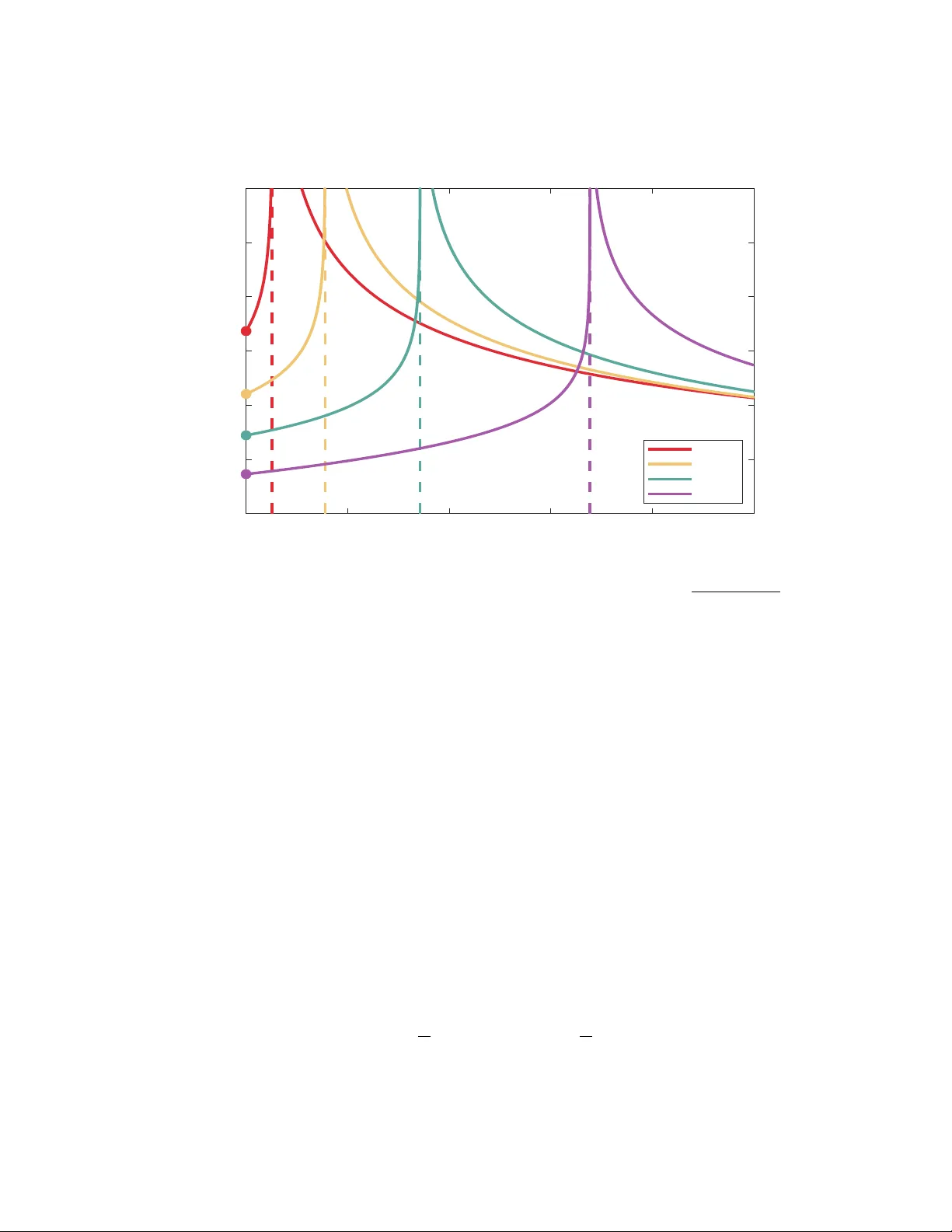
ST ABILITY OF PERIODIC W A VES IN THE MODEL WITH INTENSITY–DEPENDENT DISPERSION F ´ ABIO NA T ALI, DMITR Y E. PELINO VSKY, AND SHUO Y ANG W ANG Abstract. W e study standing p erio dic w a v es mo deled b y the nonlinear Sc hr¨ odinger equation with the in tensit y-dep enden t disp ersion co eﬃcien t. Spatial p erio dic proﬁles are smo oth if the frequency of the standing wa v es is b elow the limiting frequency , for which the proﬁles b ecome p eak ed (piecewise con tin uously diﬀeren tiable with a ﬁnite jump of the ﬁrst deriv ativ e). W e pro ve that there exist t wo families of the perio dic wa ves with smo oth proﬁles separated by a homo clinic orbit and the p erio d function (the energy-to- p erio d mapping) is monotonically increasing for the family inside the homo clinic orbit and decreasing for the family outside the homo clinic orbit. This prop erty allows us to deriv e a sharp criterion for the energetic stability of such standing p erio dic wa ves under time evolution if the p erturbations are p erio dic with the same p erio d for b oth families and, additionally , for the family outside the homo clinic orbit, spatially o dd with resp ect to the half-p erio d. By numerically approximating the sharp stability criterion, w e show that both families are energetically stable for small frequencies but become unstable when the frequency approac hes the limiting frequency of the p eaked wa ves. 1. Intr oduction W e consider the nonlinear Schr¨ odinger (NLS) equation, where the disp ersion co eﬃcien t dep ends linearly on the w av e in tensity . This mo del in one spatial dimension can b e written in the normalized form: iu t + (1 − | u | 2 ) u xx + | u | 2 u = 0 , (1.1) where u = u ( t, x ) and u : R × R → C . W e assume that u ( t, · ) is spatially perio dic with the p erio d L for any t ∈ R . If the disp ersion co eﬃcient is constant, the model is equiv alent to the cubic fo cusing NLS equation, one of the fundamen tal mo dels of nonlinear science [10, 17]. W e refer to (1.1) as the NLS–IDD e quation . 1.1. Bac kground and motiv ations. Mathematical mo dels with the in tensit y-dep enden t disp ersion terms hav e b een studied in the ph ysics of the coheren tly prepared multistate atoms [13], quantum w ell wa veguides [19], ﬁber-optics communication systems [23], and the quan tum harmonic oscillators in the presence of nonlinear eﬀective masses [4]. The NLS–IDD equation also arises as the contin uum limit of the Salerno lattice mo del [33], i∂ τ ψ n + (1 − | ψ n | 2 )( ψ n +1 + ψ n − 1 ) + µ | ψ n | 2 ψ n = 0 , (1.2) where µ ∈ R is the co eﬃcient of the onsite nonlinearity and ψ n = ψ n ( τ ) is the w av e function in ( τ , n ) ∈ R × Z . If µ = 2 + h 2 and ψ n ( τ ) = e 2 iτ u ( h 2 τ , hn ) with a smo oth 1 2 F. NA T ALI, D. E. PELINO VSKY, AND S. W ANG u = u ( t, x ), then expanding in p ow ers of the small stepsize h yields the NLS–IDD equation (1.1) from the Salerno mo del (1.2) at order O ( h 2 ). The mathematical analysis of mo del (1.1) without the lo cal cubic term | u | 2 u w as devel- op ed in [32], where it was sho wn that a contin uous family of bright solitons exists among the standing wa ve solutions. The spatial proﬁles of bright solitons ha v e tw o logarithmic singularities for the ﬁrst deriv ative and the contin uous parameter is giv en by the distance b et w een the t wo singularities. The energetic stabilit y of the brigh t solitons was obtained in [30] b y using the v ariational c haracterization of the singular proﬁles as minimizers of the mass sub ject to a ﬁxed energy . W ell-p osedness of the mo del w as not studied in [30, 32]. A similar mo del without the lo cal cubic term | u | 2 u and with the inv erted intensit y– dep enden t coeﬃcien t (1 − | u | 2 ) − 1 u xx w as considered in [28], where a family of dark solitons (tra veling wa v e solutions) w as shown to ha ve smo oth spatial proﬁles and the limiting black solitons (standing w av e solutions) were sho wn to b e energetically stable as constrained minimizers of the energy sub ject to ﬁxed mass and momen tum. Dark solitons in the quasilinear NLS equations with nonconstant disp ersion terms were considered in [20, 21, 22]. Both brigh t and dark solitons were also studied in the NLS equations with regularized disp ersion terms [1, 2, 29]. The NLS–IDD equation (1.1) was studied in [18], where the contin uous family of bright solitons is parameterized b y the frequency of the standing w av e solution u ( t, x ) = e iω t φ ( x ) with the spatially decaying poﬁle φ . The proﬁle φ smo oth for 0 < ω < 1 and p eaked (piecewise contin uously diﬀerentiable with a single jump of the ﬁrst deriv ative) for ω = 1. A sharp criterion for energetic stabilit y of bright solitons with resp ect to the spatially deca ying p erturbations in H 1 ( R ) was obtained in [18] from the v ariational c haracterization of the smooth proﬁles as local minimizers of the energy sub ject to a ﬁxed mass. The sharp criterion is given by the monotone increase of the mass with resp ect to the frequency , the latter condition is chec ked numerically . Energetic stability is equiv alen t to the orbital stability if the lo cal well-posedness of the NLS-IDD equation (1.1) can b e obtained in H 1 ( R ). Ho wev er, the state-of-the-art in the well-posedness of quasilinear NLS equations is not y et at the level of H 1 ( R ). Lo cal w ell-p osedness of the models whic h include (1.1) was prov en in Sob olev spaces of higher regularit y [15, 25, 31]. More recen tly , the lo cal well-posedness of quasilinear NLS equations w as established in H s ( R ) for s > 2 in [26] and for small data in H s ( R ) for s > 1 in [14]. Lo cal well-posedness of quasilinear NLS equations including the NLS–IDD equation (1.1) w as also extended to the p erio dic domain in Sob olev spaces of higher regularit y [7, 8, 9]. The main purp ose of this work is to study the ener getic stability of standing p erio dic waves with the smo oth pr oﬁles with r esp e ct to p erio dic p erturb ations of the same p erio d. The perio dic spatial domain is more practical for ph ysical exp erimen ts mo deled b y the NLS–IDD equation (1.1). The mathematical analysis of stability in the p erio dic setting in tro duces additional challenges b ecause the Morse index in the v ariational characteriza- tion ma y exceed a single negativ e eigenv alue. W e con trol the Morse index with a precise analysis of the monotonicit y of the p erio d function (the energy-to-p erio d mapping). Sim- ilarly to the scop es of [18], w e obtain a sharp criterion for the energetic stability of the ST ABILITY OF PERIODIC W A VES IN THE NLS-IDD MODEL 3 smo oth p erio dic w av es as local minimizers of the energy in H 1 per sub ject to ﬁxed mass, pro vided that the mass at the p erio dic w a ve proﬁle is monotonically increasing with re- sp ect to frequency ω for 0 < ω < 1. W e compute the latter criterion numerically and p oin t out inaccuracies in the previous n umerical approximations in [18] p erformed for the case of brigh t solitons. These main results of our study are describ ed next. 1.2. Main results. W e denote the space of square integrable L -p erio dic functions by L 2 per . F or s ≥ 0, the Sob olev space H s per is the set of p erio dic distributions such that ∥ f ∥ H s per := ∞ X k = −∞ (1 + | k | 2 ) s | ˆ f ( k ) | 2 ! 1 / 2 < ∞ , where ˆ f is the p erio dic F ourier transform of f (the F ourier series of f ). The space H s per is a Hilbert space with a natural inner pro duct denoted b y ⟨· , ·⟩ H s per . When s = 0, the space H s per is isometrically isomorphic to the space L 2 per , that is, L 2 per = H 0 per . The norm and inner pro duct in L 2 per are denoted b y ∥ · ∥ L 2 per and ⟨· , ·⟩ L 2 per . The time-dep endent NLS–IDD equation (1.1) admits the conserv ed energy H ( u ) and mass Q ( u ) giv en b y H ( u ) = Z T L  | u x | 2 + | u | 2 + log(1 − | u | 2 )  dx (1.3) and Q ( u ) = − Z T L log(1 − | u | 2 ) dx, (1.4) where R T L denotes the in tegral ov er the p erio dic domain T L with the spatial perio d L , whic h is indep enden t on the starting p oin t of integration. The conserved quan tities are w ell deﬁned in the set of functions X =  u ∈ H 1 per : ∥ u ∥ L ∞ < 1  . The NLS–IDD equation (1.1) also admits the conserv ed momentum P ( u ) if u  = 0, see [18]. Since the momentum does not pla y an y role in our study , we do not in tro duce it here. W e consider standing wa v es of the form u ( t, x ) = e iω t φ ( x ), where ω is the w av e fre- quency . Substituting this ansatz into (1 . 1), we obtain − (1 − φ 2 ) φ ′′ + ω φ − φ 3 = 0 , (1.5) whic h can b e rewritten as Newton’s equation for a 1D particle in a potential energy V : d 2 φ dx 2 = ( ω − φ 2 ) 1 − φ 2 φ = − dV dφ , V ( φ ) = 1 2 ( ω − φ 2 ) + 1 2 (1 − ω ) log 1 − ω 1 − φ 2 . (1.6) The total energy E of Newton’s particle is conserved along every solution of (1.6): E ( φ, φ ′ ) = 1 2 ( φ ′ ) 2 + V ( φ ) . (1.7) 4 F. NA T ALI, D. E. PELINO VSKY, AND S. W ANG The v ariational c haracterization of the spatial proﬁle φ is p ossible since the second-order equation (1.6) is the Euler–Lagrange equation for the augmented energy functional G ( u ) = H ( u ) + ω Q ( u ) , (1.8) deﬁned from the conserved energy H ( u ) and mass Q ( u ) in (1.3) and (1.4). The phase portrait in Figure 1.1 represen ts all b ounded solutions of the system (1.6) for 0 < ω < 1, see also [18]. There exist t wo families of p erio dic orbits with smo oth proﬁles separated b y a pair of homo clinic orbits. One family is inside one of the tw o homo clinic orbits with the left (negativ e) p erio dic orbits b eing symmetrically reﬂected from the right (p ositiv e) perio dic orbits due to the symmetry transformation: φ → − φ . The other family is outside the t w o homo clinic orbits and symmetrically span all four quadran ts of the phase plane. ? -1 -0.8 -0.6 -0.4 -0.2 0 0.2 0.4 0.6 0.8 1 ? 0 -0.5 -0.4 -0.3 -0.2 -0.1 0 0.1 0.2 0.3 0.4 0.5 Figure 1.1. The phase p ortrait of system (1.6) for ω = 0 . 5. The following theorem summarizes the existence properties of the tw o families of the p erio dic orbits. Theorem 1.1. Fix the sp atial p erio d L > 0 for the p erio dic domain T L and deﬁne ω L = 2 π 2 L 2 + 2 π 2 , Ω L = − 4 π 2 L 2 . F or any ω ∈ ( ω L , 1) , ther e exists a p erio dic orbit of system (1.6) with the smo oth pr oﬁle φ satisfying  0 < φ ( x ) < 1 , ∀ x ∈ T L , φ ( x − x 0 ) = φ ( x 0 − x ) , x 0 ∈ T L , ∀ x ∈ T L . (1.9) F or any ω ∈ (Ω L , 1) , ther e exists a p erio dic orbit of system (1.6) with the smo oth pr oﬁle φ satisfying  − 1 < φ ( x ) < 1 , ∀ x ∈ T L , φ ( x − x 0 ) = − φ ( x 0 − x ) = φ  L 2 − x + x 0  , x 0 ∈ T L , ∀ x ∈ T L . (1.10) ST ABILITY OF PERIODIC W A VES IN THE NLS-IDD MODEL 5 F or b oth families, x 0 is an arbitr ary tr anslational p ar ameter along the p erio dic orbit. Remark 1.2. F or simplicity of terminolo gy, we c al l the family of p erio dic orbits inside the homo clinic orbits satisfying (1.9) as the even waves and the family of p erio dic orbits outside the homo clinic orbits satisfying (1.10) as the o dd waves. Figur e 1.1 shows a former p erio dic orbit in blue and a latter p erio dic orbit in r e d to gether with its symmetric r eﬂe ction. The homo clinic orbits ar e shown by dashe d black lines. Eac h family of p erio dic orbits corresp ond to the energy level E ( φ, φ ′ ) = E given by the ﬁrst inv arian t (1.7). F or ω ∈ (0 , 1), the family of ev en w av es satisfying (1.9) corresp onds to E ∈ (0 , E ω ) and the family of o dd w av es satisfying (1.10) corresp onds to E ∈ ( E ω , ∞ ), where E ω = V (0) = 1 2 ω + 1 2 (1 − ω ) log (1 − ω ) is the energy level corresp onding to the homo clinic orbits for the saddle p oin t (0 , 0). If ω ∈ ( −∞ , 0), the family of o dd w a v es satisfying (1.10) corresp ond to E ∈ ( E ω , ∞ ), where E ω = V (0) is the energy lev el corresponding to the cen ter point (0 , 0). F or each energy lev el E ( φ, φ ′ ) = E , w e can deﬁne the p erio d function T ( E , ω ) by T ( E , ω ) = I dφ p 2( E − V ( φ )) , (1.11) where H corresp onds to the line integral taken along the closed p erio dic orbit. Figure 1.2 sho ws the dep endence of T ( E , ω ) v ersus E for ﬁxed v alues of ω ∈ (0 , 1), where the div ergence of T ( E , ω ) corresp onds to the homo clinic orbit at E = E ω . The ﬁgure suggests that, for ω ∈ (0 , 1), the mapping E → T ( E , ω ) is monotonically increasing for the ev en w av e and is monotonically decreasing for the o dd w a ve. These prop erties are formulated in the follo wing theorem. Theorem 1.3. The p erio d function T = T ( E , ω ) in (1.11) is a C 1 function of E ∈ (0 , ∞ ) \E ω if ω ∈ (0 , 1) and E ∈ ( E ω , ∞ ) if ω ∈ ( −∞ , 0) . F or any ω ∈ (0 , 1) , the mapping (0 , E ω ) ∋ E → T ( E , ω ) is monotonic al ly incr e asing. F or any ω ∈ ( −∞ , 1) , the mapping ( E ω , ∞ ) ∋ E → T ( E , ω ) is monotonic al ly de cr e asing. Due to smoothness and monotonicit y of the p erio d function in Theorem 1.3, one can uniquely deﬁne the energy level E = E L ( ω ) for an y spatial p erio d L > 0 in Theorem 1.1 from the ro ot of T ( E L ( ω ) , ω ) = L , where ω ∈ ( ω L , 1) for the even w av e and ω ∈ (Ω L , 1) for the o dd wa ve. F urthermore, the mappings ( ω L , 1) ∋ ω → E L ( ω ) and (Ω L , 1) ∋ ω → E L ( ω ) are C 1 . These smo othness prop erties play a central role in the energetic stabilit y analysis of the p erio dic wa ves. The Hessian op erator L = H ′′ ( φ ) + ω Q ′′ ( φ ) of the augmented energy functional (1.8) computed at the critical p oint with the proﬁle φ is deﬁned as L =   L + 0 0 L −   , L + = − ∂ 2 x + 1 + ( ω − 1) 1+ ϕ 2 (1 − ϕ 2 ) 2 , L − = − ∂ 2 x + 1 + ( ω − 1) 1 (1 − ϕ 2 ) , (1.12) 6 F. NA T ALI, D. E. PELINO VSKY, AND S. W ANG E 0 0.1 0.2 0.3 0.4 0.5 T 0 2 4 6 8 10 12 ! = 0 : 3 ! = 0 : 5 ! = 0 : 7 ! = 0 : 9 Figure 1.2. The p erio d function T ( E , ω ) v ersus E for ﬁxed v alues of ω . The dots denote the cutoﬀ v alue of E satisfying T ( E , ω ) = π p 2(1 − ω ) /ω for ω = ω L . The vertical lines show divergence of T ( E , ω ) at E = E ω . F or simplicity of notations, we set H s per := H s per × H s per , L 2 per := L 2 per × L 2 per , endo wed with their usual norms and scalar pro ducts. When necessary and since C can b e identiﬁed with R 2 , notations abov e can also b e used for complex-v alued functions in the follo wing sense: for f ∈ H s per w e ha ve f = f 1 + if 2 with f 1 , f 2 ∈ H s per . By studying the sp ectrum of L in L 2 per , we obtain the sharp criterion for the energetic stabilit y of the p erio dic wa v es with the spatial proﬁle φ stated in the follo wing theorem. Theorem 1.4. Fix the sp atial p erio d L > 0 as in The or em 1.1 and set x 0 = 0 . The pr oﬁle φ ∈ H 1 per is a C 1 function of ω for the even wave in ( ω L , 1) and for the o dd wave in (Ω L , 1) . F or any ω ∈ ( ω L , 1) , the even wave with the pr oﬁle φ is a lo c al minimizer of ener gy H ( u ) for a ﬁxe d mass Q ( u ) in H 1 per , which is de gener ate only due to tr anslational and r otational symmetries, if and only if the mapping ω → Q ( φ ) is monotonic al ly incr e asing. F or any ω ∈ (Ω L , 1) , the o dd wave with the pr oﬁle φ is a lo c al minimizer of ener gy H ( u ) for a ﬁxe d mass Q ( u ) in Y ⊂ H 1 per , wher e Y =  u ∈ H 1 per : u  L 2 − x  = − u  x − L 2  , ∀ x ∈ T L  , (1.13) which is only de gener ate by the r otational symmetry, if and only if the mapping ω → Q ( φ ) is monotonic al ly incr e asing. ST ABILITY OF PERIODIC W A VES IN THE NLS-IDD MODEL 7 By using accurate numerical approximations based on the ﬁrst in v arian t (1.7) and the p erio d function (1.11), w e can compute solutions of the implicit equation T ( E L ( ω ) , ω ) = L for a ﬁxed spatial p erio d L > 0 and the appro ximations of the spatial proﬁle φ of the p erio dic wa v e. Figure 1.3 shows the corresp onding results for the ev en wa v e satisfying (1.9) with x 0 = 0. The left panel plots ˜ E L ( ω ) := E L ( ω ) − E ω v ersus ω in ( ω L , 1) for L = 2 π , 3 π , 4 π and the righ t panel shows the spatial proﬁle φ = φ ( x ) v ersus x for L = 4 π and ω = 0 . 3 , 0 . 6 , 0 . 9. Numerical inaccuracies in the computations o ccur near ω = 1 and the end p oints in the n umerical data on the left panel are sho wn b y solid dots. The spatial proﬁle of the ev en p erio dic wa ve b ecomes p eaked as ω → 1. Solving (1.5) for ω = 1 yields the p eak ed proﬁle ω = 1 : φ ( x ) = cosh  L 2 − | x |  cosh  L 2  , x ∈  − L 2 , L 2  , (1.14) whic h is sho wn on the right panel b y dashed line. The corresp onding energy level can b e computed as E L ( ω = 1) = − 1 2 cosh 2  L 2  , (1.15) whic h is sho wn on the left panel b y open dots. An interpolation b et w een the righ t solid dot and the op en dot for (1.15) is sho wn by dotted line. ! 0 0.2 0.4 0.6 0.8 1 ~ E L -0.035 -0.03 -0.025 -0.02 -0.015 -0.01 -0.005 0 L = 2 : L = 3 : L = 4 : x -5 0 5 ? 0 0.2 0.4 0.6 0.8 1 ! = 0 : 3 ! = 0 : 6 ! = 0 : 9 ! = 1 Figure 1.3. Numerical approximations for the even w av es satisfying (1.9) with x 0 = 0. Left: the dep endence of ˜ E L v ersus ω for L = 2 π , 3 π , 4 π . Right: the spatial proﬁle φ versus x for ω = 0 . 3 , 0 . 6 , 0 . 9 and L = 4 π . Figure 1.4 shows the corresp onding results for the odd w av e satisfying (1.10) with x 0 = 0 for ω ∈ (Ω L , 1) with Ω L < 0. W e note the non-monotone dep endence of ˜ E L ( ω ) := E L ( ω ) − E ω v ersus ω on the left panel, whic h is not an obstacle to our analysis. The spatial 8 F. NA T ALI, D. E. PELINO VSKY, AND S. W ANG proﬁle of the p erio dic w av e b ecomes p eaked as ω → 1. Solving (1.5) for ω = 1 yields the o dd spatial proﬁle in the form: ω = 1 : φ ( x ) =                  − sinh  L 2 + x  sinh  L 4  x ∈  − L 2 , − L 4  sinh x sinh  L 4  x ∈  − L 4 , L 4  sinh  L 2 − x  sinh  L 4  x ∈  L 4 , L 2  , (1.16) whic h is sho wn on the right panel b y dashed line. The corresp onding energy level can b e computed as E L ( ω = 1) = 1 2 sinh 2  L 2  , (1.17) whic h is shown on the left panel by op en dots. The end p oints in the n umerical data on the left panel are shown by solid dots. An interpolation betw een the right solid dot and the op en dot for (1.17) is shown by dotted line. ! -1 -0.5 0 0.5 1 ~ E L 0 0.05 0.1 0.15 0.2 L = 2 : L = 3 : L = 4 : x -5 0 5 ? -1 -0.5 0 0.5 1 ! = 0 : 3 ! = 0 : 6 ! = 0 : 9 ! = 1 Figure 1.4. Numerical appro ximations for the odd wa v es satisfying (1.10) with x 0 = 0. Left: the dep endence of ˜ E L v ersus ω for L = 2 π , 3 π , 4 π . Right: the spatial proﬁle φ versus x for ω = 0 . 3 , 0 . 6 , 0 . 9 and L = 4 π . By using the n umerical approximation of the spatial proﬁle φ , we can also compute the mass Q ( φ ) for a ﬁxed spatial perio d L > 0 and plot it v ersus ω to v erify the sharp criterion for the energetic stabilit y of the perio dic wa v es giv en by Theorem 1.4. Figure 1.5 plots Q ( φ ) v ersus ω for L = 2 π , 3 π , 4 π . The dashed line shows the dep endence of Q ( φ ) in the limit L → ∞ , which corresp onds to the solitary w av es. The left panel presents the ST ABILITY OF PERIODIC W A VES IN THE NLS-IDD MODEL 9 mapping ω → Q ( φ ) for the even w a ve satisfying (1.9) and the righ t panel presen ts the same for the odd wa v e satisfying (1.10). The numerical inaccuracies o ccur near ω = 1 and the end p oin ts of the numerical data are shown by solid dots. By using (1.14) and (1.16), w e are able to compute Q ( φ ) analytically at ω = 1 for the p eaked wa v es, see (6.4) and (6.6) below, and sho w the result in Figure 1.5 b y open dots. An in terp olation betw een the righ t solid dot and the op en dot is shown by dotted line. ! 0 0.2 0.4 0.6 0.8 1 Q 0 0.5 1 1.5 2 2.5 3 ! -1 -0.5 0 0.5 1 Q 0 1 2 3 4 5 L = 2 : L = 3 : L = 4 : L ! 1 Figure 1.5. Dep endence of Q ( φ ) v ersus ω for L = 2 π , 3 π , 4 π and in the limit L → ∞ (dashed line). Left panel: the ev en w a ve satisfying (1.9). Righ t panel: the o dd wa v e satisfying (1.10). Based on the numerical approximations and the sharp criterion in Theorem 1.4, w e conclude from Figure 1.5 that b oth even and o dd perio dic w av es are energetically stable for smaller v alues of ω and energetically unstable for v alues of ω near ω = 1. T o b e precise, w e form ulate the following conjecture. Conjecture 1.5. Ther e is ω ∗ ∈ ( ω L , 1) and Ω ∗ ∈ (0 , 1) such that the even wave satisfying (1.9) is ener getic al ly stable for ω ∈ ( ω L , ω ∗ ) and unstable for ω ∈ ( ω ∗ , 1) , wher e as the o dd wave satisfying (1.10) is ener getic al ly stable for ω ∈ (Ω L , Ω ∗ ) and unstable for ω ∈ (Ω ∗ , 1) . Remark 1.6. The numeric al data in Figur es 1.2, 1.3, 1.4, and 1.5 ar e obtaine d with high numeric al ac cur acy, c ontr ol le d within 10 − 8 err or, sinc e the numeric al err or only arises in the c omputation of the p erio d function T ( E , ω ) and the wave pr oﬁle φ ( x ) fr om the c orr esp onding inte gr als. The dep endenc e of Q ( φ ) versus ω in the limit L → ∞ shown in Figur e 1.5 c ontr adicts the claim fr om [18, Figure 5] that the dep endenc e is monotonic al ly incr e asing ne ar ω = 0 and ω = 1 and de cr e asing for ω ∈ ( ω 1 , ω 2 ) for some 0 < ω 1 < ω 2 < 1 . A lthough the numeric al data on Q ( φ ) versus ω in [18] was c onsistent with the numeric al appr oximations of unstable eigenvalues in the sp e ctr al stability pr oblem, se e same Figur e 5 in [18] , we have found that the claim of stability of bright solitons ne ar ω = 1 in [18] is a numeric al artefact. It is r elate d with the c enter-diﬀer enc e appr oximations of the se c ond- or der derivatives with a lar ge stepsize, which wer e use d in [18] . By r e ducing the stepsize 10 F. NA T ALI, D. E. PELINO VSKY, AND S. W ANG or p erforming c omputations with adaptive metho ds dir e ctly fr om (1.7) and (1.11), we have found that Q ( φ ) is monotonic al ly de cr e asing in ω ne ar ω = 1 . A lthough our numeric al data has a tiny gap ne ar ω = 1 due to the lack of numeric al ac cur acy, c omp arison b etwe en the last numeric al data (solid right dots) and the analytic al ly c ompute d limiting value of Q ( φ ) at ω = 1 (op en dots) suggest the monotone de cr e ase of Q ( φ ) ne ar ω = 1 . 1.3. Metho dology and organization of the paper. The existence of p erio dic orbits stated in Theorem 1.1 is ob vious from the phase p ortrait shown in Figure 1.1. Neverthe- less, w e complemen t this dynamical system picture with the functional-analytic setup and pro ve the existence of p erio dic orbits based on the implicit function theorem. The family of ev en w av es satisfying (1.9) with x 0 = 0 is studied in a subspace of the Sob olev space H s per , s ≥ 0 constituted b y even p erio dic functions and denoted b y H s per , e . The family of odd w a ves satisfying (1.10) with x 0 = 0 is studied in a subspace constituted b y o dd p erio dic functions and denoted by H s per , o . These results are describ ed in Section 2. The monotonicit y of the p erio d function stated in Theorem 1.3 is prov en with tw o diﬀeren t methods for the even and o dd w a v es. F or the ev en w av e, w e use Chicone’s theorem [5] and conﬁrm the monotonicity criterion based on the explicit analysis of the logarithmic and p olynomial functions. F or the o dd wa ve, we estimate the p erio d function b y using conv exity of the integrand functions. These results are describ ed in Section 3. The energetic stabilit y criterion stated in Theorem 1.4 is pro v en in tw o steps. As a ﬁrst step, we analyze the Morse and nullit y indices of the Sc hr¨ odinger op erators L ± : H 2 per ⊂ L 2 per → L 2 per giv en b y (1.12), where the Morse index denoted by n ( L ± ) is the n umber of negativ e eigenv alues with the account of their multiplicities and the nullit y index denoted by z ( L ± ) is the multiplicit y of the zero eigen v alue. F or the even wa ve, we pro ve that n ( L + ) = z ( L + ) = z ( L − ) = 1 and n ( L − ) = 0. F or the o dd wa v e, we prov e that n ( L + ) = 2, n ( L − ) = z ( L + ) = z ( L − ) = 1. These results are describ ed in Section 4. As a second step, w e analyze the Morse and n ullity indices of the constrained op erator L + | { ϕ 0 } ⊥ , where the constrain t with φ 0 ≡ ϕ 1 − ϕ 2 is due to the ﬁxed mass Q restriction [12]. W e show that n ( L + | { ϕ 0 } ⊥ ) = 0 and z ( L + | { ϕ 0 } ⊥ ) = 1 for the ev en w a ve if and only if the mapping ω → Q ( φ ) is monotonically increasing, which yields Theorem 1.4 for the even w a ve. W e also sho w that n ( L + | { ϕ 0 } ⊥ ) = 1 and z ( L + | { ϕ 0 } ⊥ ) = 1 for the o dd w a ve if and only if the mapping ω → Q ( φ ) is monotonically increasing. This is still inconclusive for the energetic stability of the o dd wa v e. How ever, restricting H 1 per to the space Y of o dd p erturbations with resp ect to the half-p erio d allo ws us to obtain n ( L + | { ϕ 0 } ⊥ ∩Y ) = n ( L − | Y ) = 0 and z ( L + | { ϕ 0 } ⊥ ∩Y ) = z ( L − | Y ) = 1 if and only if the mapping ω → Q ( φ ) is monotonically increasing, whic h yields Theorem 1.4 for the o dd wa v e. These results are described in Section 5. W e note that the idea of restricting the space of p erio dic functions to o dd p erturbations with resp ect to the half-p erio d is prop osed in [11] for the stabilit y analysis of o dd w a ves in the cubic NLS equation. Finally , the numerical metho ds used to compute the data in Figures 1.2, 1.3, 1.4, and 1.5 are describ ed in Section 6. W e also elab orate Remark 1.6 ab out the limit L → ∞ with more details. ST ABILITY OF PERIODIC W A VES IN THE NLS-IDD MODEL 11 2. Existence of periodic w a ves W e prov e Theorem 1.1 within a functional analysis framework. Section 2.1 deﬁnes the basic facts used in the pro ofs. Sections 2.2 and 2.3 pro vide global con tin uations of the ev en and o dd w av es for the ﬁxed spatial p erio d L > 0. 2.1. Preliminary facts. W e ﬁrst recall some facts regarding F redholm op erators on a Banac h space X . An un b ounded op erator S : D ( S ) ⊂ X → X is called a F r e dholm op er ator if Range( S ) is closed and dim( Ker( S )) and dim(Cok er( S )) are both ﬁnite, where Cok er( S ) denotes the quotien t space given by Cok er( S ) = X  Range( S ) . The index of an un b ounded F redholm op erator S : D ( S ) ⊂ X → X is giv en b y ind( S ) = dim( Ker( S )) − dim(Coker( S )) ∈ Z . A F redholm op erator is of index zero if ind( S ) = 0. The follo wing lemma pro vides a result that is useful for our purp oses since we obtain a suitable relation b etw een c ( S ) = dim(Cok er( S )) and z ( S ) = dim( Ker( S )). Lemma 2.1. L et H b e a r e al Hilb ert sp ac e and let K ⊂ H b e a close d subsp ac e. Then, H / K ∼ = K ⊥ . Pr o of. Let us deﬁne T : H / K → K ⊥ giv en b y T ( u ) = u − P K u for an y u ∈ H , where P K is the orthogonal pro jection from H onto the closed subspace K . Since ||T ( u ) || H = || u − P K u || , w e obtain b y the Pythagorean theorem || u || 2 H = || P K u || 2 H + || u − P K u || 2 H = || P K u || 2 H + ||T ( u ) || 2 H . The equalit y implies ||T ( u ) || 2 H = || u || 2 H − || P K u || 2 H ≤ || u || 2 H , and thus, T is a b ounded op erator. T is a one-to-one op erator since T ( u ) = 0 implies u = P K u and this fact automatically implies u ∈ K . T o show that T is onto, we consider v ∈ K ⊥ . By the deﬁnition of orthogonal pro jection from H on to the closed subspace K , there exists u ∈ H suc h that v = u − P K u , and T is onto as desired. ■ Remark 2.2. If S : D ( S ) ⊂ H → H is an unb ounde d self-adjoint line ar op er ator with a close d r ange on a Hilb ert sp ac e H , then we have by L emma 2 . 1 that H  Range( S ) = H  Ker( S ) ⊥ ∼ = Ker( S ) ⊥⊥ = Ker( S ) . Ther efor e, if dim( Ker( S )) is ﬁnite, then S is always a F r e dholm op er ator of index zer o. W e conclude this section by stating a v ersion of the implicit function theorem used in our study , see [3, Theorem 8.3.1]. Theorem 2.3. Supp ose that X and Y ar e Banach sp ac es, that F : X × R → Y is of class C k , k ≥ 2 , and that F ( x 0 , λ 0 ) = 0 ∈ Y for some ( x 0 , λ 0 ) ∈ X × R . Supp ose also that (1) ∂ g F ( g , λ ) is a F r e dholm op er ator of index zer o when F ( g , λ ) = 0 for al l ( g , λ ) ∈ U . Her e U ⊂ X × R denotes an op en subset. (2) F or some ( x 0 , λ 0 ) ∈ X × R , ker( L λ 0 ) is one dimensional, wher e L λ 0 = ∂ g F ( x 0 , λ 0 ) . This me ans that k er( L λ 0 ) = { h ∈ X ; h = sh 0 for some s ∈ R } , h 0 ∈ X \{ 0 } . (3) The tr ansversality c ondition holds: ∂ 2 λ,g F [( x 0 , λ 0 )](1 , h 0 ) / ∈ Range( L λ 0 ) . 12 F. NA T ALI, D. E. PELINO VSKY, AND S. W ANG Then, ther e exists a 0 > 0 and a br anch of solutions { ( χ ( a ) , Λ( a )); a ∈ ( − a 0 , a 0 ) } ⊂ X × R , such that Λ(0) = λ 0 and χ (0) = x 0 . In addition, we have • F ( χ ( a ) , Λ( a )) = 0 for al l a ∈ ( − a 0 , a 0 ) . • a 7→ Λ( a ) and a 7→ χ ( a ) ar e of class C k − 1 on ( − a 0 , a 0 ) . • ther e exists an op en set U 0 ⊂ X × R such that ( x 0 , λ 0 ) ∈ U 0 and { ( g , λ ) ∈ U 0 ; F ( g , λ ) = 0 , g  = 0 } = { ( χ ( a ) , Λ( a )); a ∈ ( − a 0 , a 0 ) } . • If F is analytic, then χ and Λ ar e analytic functions on ( − a 0 , a 0 ) . 2.2. Existence of (p ositiv e) even perio dic w av es. T o prov e the existence of ev en p erio dic w av es, w e consider the subspace L 2 per , e con tained in L 2 per , whic h consists of ev en p erio dic functions, that is, functions in the Hilbert space L 2 per , e =  f ∈ L 2 per : f ( − x ) = f ( x ) a . e . x ∈  − L 2 , L 2  , where the spatial p erio d L > 0 is ﬁxed. The ﬁrst result establishes a lo cal bifurcation of small (p ositive) even p erio dic wa ves from the (p ositiv e) constan t solution φ = √ ω of the second-order equation (1.5). Prop osition 2.4. Ther e exists a 0 > 0 such that for al l a ∈ ( − a 0 , a 0 ) ther e exists an even p erio dic solution φ ∈ H 2 per , e to the se c ond-or der e quation (1.5) given by φ ( x ) = √ ω + ∞ X n =1 φ n ( x ) a n , (2.1) wher e { φ n } n ∈ N ar e uniquely determine d in H 2 per , e . The fr e quency ω of the L -p erio dic wave is given by ω = ω L + ∞ X n =1 ω 2 n a 2 n , (2.2) wher e ω L = 2 π 2 L 2 +2 π 2 and { ω 2 n } n ∈ N ar e uniquely determine d c onstants. F urthermor e, we have ω > ω L for smal l a  = 0 . Pr o of. W e outline the steps used to pro ve the existence of small–amplitude perio dic w a ves using Theorem 2 . 3. Let F : H 2 per , e × R → L 2 per , e b e the smo oth map deﬁned by F ( g , λ ) = − (1 − g 2 ) g ′′ + λg − g 3 . W e see that F ( g , λ ) = 0 if and only if g ∈ H 2 per , e satisﬁes (1 . 5) with corresponding frequency λ = ω ∈ R . Let λ 0 > 0 b e ﬁxed. The F r´ echet deriv ativ e of the function F with resp ect to the ﬁrst v ariable at ( √ λ 0 , λ 0 ) is giv en b y D g F ( p λ 0 , λ 0 ) f = − (1 − λ 0 ) f ′′ − 2 λ 0 f . The non trivial k ernel of D g F ( √ λ 0 , λ 0 ) is determined by functions h ∈ H 2 per , e suc h that b h ( n ) (1 − λ 0 )  2 π n L  2 − 2 λ 0 ! = 0 , n ∈ N \{ 0 } , ST ABILITY OF PERIODIC W A VES IN THE NLS-IDD MODEL 13 where b h ( n ) is the n -th co eﬃcient of the F ourier series of h ∈ L 2 per . W e see that D g F ( √ λ 0 , λ 0 ) has nontrivial kernel if, and only if, λ 0 = ( 2 πn L ) 2 2+ ( 2 πn L ) 2 > 0 for some n ∈ N \{ 0 } . In this case, w e ha ve Ker D g F ( p λ 0 , λ 0 ) = Span( e ϕ n ) , e ϕ n ( x ) = cos  2 π n L x  , n ∈ N \{ 0 } . In addition, since D g F ( √ λ 0 , λ 0 ) is a self-adjoin t op erator deﬁned in L 2 per , e with domain H 2 per , e , the transv ersalit y condition is also satisﬁed: cos  2 π n L x  / ∈ Ker D g F ( p λ 0 , λ 0 ) ⊥ = Range D g F ( p λ 0 , λ 0 ) . T o obtain p erio dic solutions with minimal spatial perio d L > 0, we m ust consider n = 1. Thus, we hav e λ 0 = 2 π 2 L 2 +2 π 2 = ω L and deﬁne the set S given by S = { ( g , λ ) ∈ U ; F ( g , λ ) = 0 } , where U =  ( g , λ ) ∈ H 2 per,e × ( λ 0 , 1) ; 0 < g < 1  . Let ( g , λ ) ∈ S b e a solution of the equation F ( g, λ ) = 0. First, w e pro v e that the linear op erator D g F ( g , λ ) = − (1 − g 2 ) ∂ 2 x + λ − 3 g 2 + 2 g g ′′ is a F redholm op erator of index zero. In fact, in order to simplify the notation, let us denote Q = D g F ( g , λ ) and P = (1 − g 2 ) − 1 Q. First, P is clearly a self-adjoin t operator. Thus, σ ( P ) = σ disc ( P ) ∪ σ ess ( P ), where σ ( P ) denotes the sp ectrum of P , and σ disc ( P ) and σ ess ( P ) denote, resp ectiv ely , the discrete and essential sp ectra of P . Since H 2 per , e is compactly em b edded in L 2 per , e , the op erator P has compact resolven t. Consequently , σ ess ( P ) = ∅ , and σ ( P ) = σ disc ( P ) consists of isolated eigen v alues with ﬁnite algebraic multiplicities (see e.g., [16, Section I I I.6]). Since ( g , λ ) ∈ S , w e see that 0 is an eigenv alue for P asso ciated with the eigenfunction g ′ and z ( P ) is ﬁnite. A basis for the subspace Ker( P ) can b e taken as { v 1 , · · · , v n } . On one hand, by Remark 2 . 2 we hav e L 2 per , e  Range( Q ) ∼ = Range( Q ) ⊥ = Ker( Q ∗ ) = Ker( P (1 − g 2 )) . Since { v 1 (1 − g 2 ) − 1 , · · · , v n (1 − g 2 ) − 1 } is a basis for the subspace Ker( Q ∗ ), it follo ws that z ( P ) = z ( Q ∗ ), and z ( Q ∗ ) is ﬁnite. On the other hand, w e ha ve Ker( P ) = Ker( Q ), so that z ( Q ∗ ) = z ( P ) = z ( Q ) and the index of the F redholm op erator Q is zero as desired. Th us, b y deﬁning λ 0 = ω L ∈ (0 , 1), the lo cal bifurcation theory established in The- orem 2 . 3 guaran tees the existence of an op en interv al I ⊂ (0 , 1) near ω L , an op en ball B ( √ ω L , r ) ⊂ H 2 per , e , around the equilibrium solution √ ω L , for some r > 0 and a smooth mapping ω ∈ I 7→ φ ∈ B ( √ ω L , r ) ⊂ H 2 per , e , (2.3) 14 F. NA T ALI, D. E. PELINO VSKY, AND S. W ANG suc h that F ( φ, ω ) = 0 for all ω ∈ I and φ ∈ B ( √ ω L , r ). Next, we determine the ﬁrst terms in the expansions (2 . 1) and (2 . 2). T o simplify the notation, let us deﬁne s = √ ω L . The T aylor expansion of the square-ro ot function at ω L yields √ ω = s + ω 2 2 s a 2 + O ( a 4 ) . The correction terms ω 2 and { φ 1 , φ 2 , φ 3 } are uniquely determined by the following recur- rence relations        O ( a ) : − (1 − s 2 ) φ ′′ 1 − 2 s 2 φ 1 = 0 , O ( a 2 ) : − (1 − s 2 ) φ ′′ 2 − 2 s 2 φ 2 + 2 sφ 1 φ ′′ 1 − 3 sφ 2 1 = 0 , O ( a 3 ) : − (1 − s 2 ) φ ′′ 3 − 2 s 2 φ 3 + ω 2 ( φ ′′ 1 − 2 φ 1 ) + 2 s ( φ 1 φ ′′ 2 + φ 2 φ ′′ 1 ) − 6 sφ 1 φ 2 − φ 3 1 + φ 2 1 φ ′′ 1 = 0 . (2.4) W e see that φ 1 ( x ) = cos( k x ) satisﬁes the equation containing the term O ( a ) for k = 2 π L since ω L = 2 π 2 L 2 +2 π 2 . Solving the inhomogeneous equation for O ( a 2 ), w e obtain φ 2 ( x ) = s 2 + 3 12 s (1 − s 2 ) (cos(2 k x ) − 3) . W e need to ﬁnd the constan t ω 2 in the third equation of (2 . 4). The inhomogeneous equation at O ( a 3 ) admits a solution φ 3 ∈ H 2 per , e if, and only if, the righ t-hand side is orthogonal to φ 1 , whic h selects uniquely the correction ω 2 = s 4 + 6 s 2 − 9 6( s 2 − 1) = 9 − 6 ω L − ω 2 L 6(1 − ω L ) . Since ω 2 > 0, the solution (2.1) with (2.2) exists for ω > ω L near ω L . This ﬁnishes the pro of of the prop osition. ■ Remark 2.5. The bifur c ating solution obtaine d in Pr op osition 2 . 4 is unique in H 2 per , e , up to the p ar ametrization pr ovide d by the bifur c ation p ar ameter. This uniqueness is ensur e d sinc e the Lyapunov–Schmidt r e duction r e quir es the applic ation of the implicit function the or em. In the c ase of a one-dimensional kernel, the bifur c ation o c curs along a single br anch of solutions. The implicit function the or em then guar ante es the existenc e of a unique smo oth curve of solutions that bifur c ates fr om the c onstant solution. The next result establishes a global con tin uation of (p ositiv e) even p erio dic w av es from the lo cal bifurcating solution obtained in Prop osition 2.4. Prop osition 2.6. The lo c al solution obtaine d in Pr op osition 2 . 4 is glob al, that is, φ exists for al l ω ∈ ( ω L , 1) . In addition, the p air ( φ, ω ) ∈ H 2 per , e × ( ω L , 1) is c ontinuous with r esp e ct to the p ar ameter ω ∈ ( ω L , 1) and it satisﬁes (1 . 5) . Pr o of. T o extend the lo cal curve in (2 . 3) to a global curve, w e need to prov e that every b ounded and closed subset R ⊂ S is a compact set con tained in H 2 per , e × ( ω L , 1). T o this end, w e w ant to prov e that R is sequentially compact, that is, if { ( φ m , ω m ) } m ∈ N is a ST ABILITY OF PERIODIC W A VES IN THE NLS-IDD MODEL 15 sequence in R , there exists a subsequence of { ( φ m , ω m ) } m ∈ N that con v erges to a p oint in R . Up to a subsequence, w e obtain ω m → ω in [ ω L , 1] , (2.5) and φ m  φ in H 2 per , e , (2.6) as m → + ∞ . Next, { φ m } is a b ounded sequence in H 2 per , e and it satisﬁes 0 < φ m < 1. Since the embedding H 2 per , e  → H 1 per , e is compact and H 1 per , e is a Banach algebra, w e obtain φ 3 m → φ 3 in H 1 per , e as m → + ∞ . In particular, w e hav e φ 2 m → φ 2 in H 1 per , e  → C per , e and b y (2 . 6), we obtain (1 − φ 2 m ) φ ′′ m  (1 − φ 2 ) φ ′′ in L 2 per , e , (2.7) as m → + ∞ . Since in particular φ 3 m → φ 3 in L 2 per , e as m → + ∞ , w e obtain b y (2 . 5) and (2 . 7) that the pair ( φ, ω ) ∈ H 2 per , e × [ ω L , 1] satisﬁes − (1 − φ 2 ) φ ′′ + ω φ − φ 3 = 0 . (2.8) W e see from (2 . 8) that ω < 1, since smooth p erio dic solutions to this equation do not exist when ω = 1. Moreo v er, if ω = ω L , the constant solution φ = √ ω L is the only solution to (2 . 8). Th us ω ∈ ( ω L , 1) as requested and we hav e φ > 0. On the other hand, if there exists t 0 ∈ [0 , L ] such that lim t → t 0 φ ( t ) = 1, then ω = 1, whic h is a con tradiction, since in this case there are no p erio dic solutions of (2 . 8). Therefore, w e obtain 0 < φ < 1 as requested. Finally , by (2 . 2) the frequency ω of the p erio dic wa v e is not constant. By applying [3, Theorem 9.1.1] we can extend globally the lo cal bifurcation curv e giv en in (2 . 3). More precisely , there is a con tinuous mapping ω ∈ ( ω L , 1) 7→ φ ∈ H 2 per , e , where φ solv es equation (2 . 8). ■ Remark 2.7. Sinc e φ is c ontinuous, satisﬁes 0 < φ < 1 , and ther e is no t ± ∈ [0 , L ] such that lim t → t − φ ( t ) = 0 and lim t → t + φ ( t ) = 1 , we obtain that ther e exist m and M that dep end on ω ∈ ( ω L , 1) such that 0 < m < M < 1 and m < φ ( x ) ≤ M for every x ∈ [0 , L ] . In fact, sinc e φ is c ontinuous on the c omp act set [0 , L ] , we have m = min [0 ,L ] φ ( x ) , M = max [0 ,L ] φ ( x ) . Prop ositions 2.4 and 2.6, as well as Remark 2.7, justify the existence result stated in Theorem 1.1 for the even wa v e satisfying (1.9) with x 0 = 0. 2.3. Existence of odd perio dic wa v es. T o pro v e the existence of o dd p erio dic w av es, w e consider the subspace L 2 per , o con tained in L 2 per , whic h consists of o dd p erio dic functions, that is, L 2 per , o =  f ∈ L 2 per : f ( − x ) = − f ( x ) a . e . x ∈  − L 2 , L 2  , 16 F. NA T ALI, D. E. PELINO VSKY, AND S. W ANG where the spatial p erio d L > 0 is ﬁxed. The ﬁrst result gives a lo cal bifurcation of small o dd p erio dic wa ves from the zero solution φ = 0 of the second-order equation (1.5). Prop osition 2.8. Ther e exists a 0 > 0 such that for al l a ∈ ( − a 0 , a 0 ) ther e exists an o dd p erio dic solution φ ∈ H 2 per , o to the se c ond-or der e quation (1 . 5) given by φ ( x ) = ∞ X n =1 φ 2 n − 1 ( x ) a 2 n − 1 , (2.9) wher e { φ n } n ∈ N ar e uniquely determine d functions in L 2 per , o . The fr e quency ω of the L - p erio dic wave is given by ω = Ω L + ∞ X n =1 ω 2 n a 2 n , (2.10) wher e Ω L = − 4 π 2 L 2 and { ω 2 n } n ∈ N ar e uniquely determine d c onstants. F urthermor e, we have ω > Ω L for smal l a  = 0 . Pr o of. The pro of is similar to that of Prop osition 2 . 4 and therefore, w e only outline the main steps. Indeed, let G : H 2 per , o × R → L 2 per , o b e the smo oth map deﬁned by G ( g , λ ) = − (1 − g 2 ) g ′′ + λg − g 3 . W e see that G ( g, λ ) = 0 if, and only if, g ∈ H 2 per , o satisﬁes (1 . 5) with corresponding frequency λ = ω ∈ R . Let λ 0 ∈ R b e ﬁxed. The F r´ ec het deriv ative of the function G with resp ect to the ﬁrst v ariable at (0 , λ 0 ) is then given by D g G (0 , λ 0 ) f = − f ′′ + λ 0 f . The non trivial k ernel of D g G (0 , λ 0 ) is determined by functions h ∈ H 2 per , o suc h that b h ( n ) −  2 π n L  2 + λ 0 ! = 0 , n ∈ N \{ 0 } . Since D g G (0 , λ 0 ) has non trivial k ernel if and only if λ 0 = −  2 π n L  2 < 0 for some n ∈ N \{ 0 } , w e ha ve Ker D g G (0 , λ 0 ) = [ e ϕ n ] , e ϕ n ( x ) = sin  2 π n L x  , n ∈ N \{ 0 } . T o obtain p erio dic solutions with the minimal spatial p erio d L > 0, we m ust consider n = 1. Thus, we hav e λ 0 = − 4 π 2 L 2 = Ω L . The remainder of the pro of is iden tical to the one in Proposition 2 . 4 but in order to complete the proof, w e shall compute the ﬁrst terms in the expansions (2 . 9) and (2 . 10). Indeed, for k = 2 π L the corrections terms ω 2 and { φ 1 , φ 3 } are uniquely determined b y the follo wing recurrence relations  O ( a ) : − φ ′′ 1 − k 2 φ 1 = 0 , O ( a 3 ) : − φ ′′ 3 − k 2 φ 3 + ω 2 φ 1 + φ 2 1 φ ′′ 1 − φ 3 1 = 0 . (2.11) W e see that φ 1 ( x ) = sin( k x ) satisﬁes the equation containing the term O ( a ). T o ﬁnd the constant ω 2 in the second equation of (2 . 11), w e use the fact that the inhomogeneous ST ABILITY OF PERIODIC W A VES IN THE NLS-IDD MODEL 17 equation at O ( a 3 ) admits a solution φ 3 ∈ H 2 per , o if, and only if, the right-hand side is orthogonal to φ 1 , whic h selects uniquely the correction ω 2 = 3 4 (1 + k 2 ) . Since ω 2 > 0, the solution (2.9) with (2.10) exists for ω > Ω L near Ω L . Finally , we solve the inhomogeneous equation for O ( a 3 ) and obtain φ 3 ( x ) = − 1 + k 2 32 k 2 sin(3 k x ) . This ﬁnishes the pro of of the prop osition. ■ Remark 2.9. Using analo gous c omputations as in Pr op osition 2 . 6 , we c an establish that the lo c al solution obtaine d in Pr op osition 2 . 8 is glob al, that is, φ exists for al l ω ∈ (Ω L , 1) . In addition, the p air ( φ, ω ) ∈ H 2 per , o × (Ω L , 1) is c ontinuous with r esp e ct to the p ar ameter ω ∈ (Ω L , 1) and it satisﬁes (1 . 5) . F urthermor e, ther e exists M that dep ends on ω ∈ (Ω L , 1) such that − 1 < − M < 0 < M < 1 and M = max [0 ,L ] φ ( x ) = − min [0 ,L ] φ ( x ) . Prop osition 2.8 and Remark 2.9 justify the existence result stated in Theorem 1.1 for the o dd wa v e satisfying (1.10) with x 0 = 0. 3. Monotonicity of the period function W e prov e Theorem 1.3 by analysing the p erio d function T = T ( E , ω ) introduced in (1.11). The p erio d function is asso ciated with the p erio dic orbits on the phase plane for the system of ordinary diﬀerential equations    φ ′ = ξ , ξ ′ = ω ϕ 1 − ϕ 2 − ϕ 3 1 − ϕ 2 . (3.1) It follo ws from the theory of ordinary diﬀerential equations that the solution φ dep ends smo othly on the parameter E = E ( φ, φ ′ ), where the energy function is E ( φ, φ ′ ) = 1 2 ( φ ′ ) 2 + V ( φ ) , V ( φ ) = 1 2 ( ω − φ 2 ) + 1 2 (1 − ω ) log 1 − ω 1 − φ 2 . (3.2) F or ω ∈ (0 , 1), the even wa v e satisfying (1.9) corresp onds to E ∈ (0 , E ω ) and the o dd w av e satisfying (1.10) corresp onds to E ∈ ( E ω , ∞ ), where E ω = E (0 , 0) corresp onds to the energy lev el of the pair of homo clinic orbits from the saddle p oint (0 , 0) whic h surround the cen ter p oin ts ( ± √ ω , 0). W e note that V ( ± √ ω ) = 0 and lim ϕ →± 1 V ( φ ) = + ∞ . F urthermore, V ( φ ) ≥ 0 for all φ ∈ [ − 1 , 1] and V ′ ( φ ) > 0 for all φ ∈ ( √ ω , 1). Section 3.1 giv es the pro of of ∂ E T ( E , ω ) > 0, E ∈ (0 , E ω ) for the p erio dic orbits inside the homo clinic orbit (the ev en w av es). Section 3.2 giv es the pro of of ∂ E T ( E , ω ) < 0, 18 F. NA T ALI, D. E. PELINO VSKY, AND S. W ANG E ∈ ( E ω , ∞ ) for the p erio dic orbits outside the pair of homo clinic orbits (the o dd wa v es). The latter result also holds for ω ∈ ( −∞ , 0) and E ∈ ( E ω , ∞ ), for whic h E ω = E (0 , 0) corresp onds to the energy level of the center p oint (0 , 0). 3.1. Monotonicit y for even p erio dic w av es. By the main theorem in [5], the p erio d function T ( E , ω ) is monotonically increasing in E in (0 , E ω ) if I ′′ ( φ ) > 0 for φ ∈ (0 , 1), where I ( φ ) = V ( φ ) [ V ′ ( φ )] 2 . (3.3) Note that the theorem in [5] can b e applied b ecause V ( √ ω ) = 0 is prop erly normalized at the cen ter p oint ( √ ω , 0). Computing V ′ ( φ ) = − φ ( ω − φ 2 ) 1 − φ 2 , V ′′ ( φ ) = − ω + ( ω − 3) φ 2 + φ 4 (1 − φ 2 ) 2 , V ′′′ ( φ ) = 2(1 − ω ) φ ( φ 2 + 3) (1 − φ 2 ) 3 , w e obtain from (3.3) that I ′′ ( φ ) = 6 V ( V ′′ ) 2 − 2 V V ′ V ′′′ − 3( V ′ ) 2 V ′′ ( V ′ ) 4 =: P ( φ ) ( V ′ ( φ )) 4 (1 − φ 2 ) 4 , (3.4) where P ( φ ) = 3 φ 2 ( ω − φ 2 ) 2 A ( φ ) +  3 A ( φ ) 2 + 2(1 − ω ) φ 2 (3 + φ 2 )( ω − φ 2 )  B ( φ ) , with A ( φ ) := ω + ( ω − 3) φ 2 + φ 4 , B ( φ ) := ω − φ 2 + (1 − ω ) log 1 − ω 1 − φ 2 . Since P dep ends on φ 2 , w e in tro duce t = φ 2 and redeﬁne P , A , and B as functions of t : P ( t ) = 3 t ( ω − t ) 2 A ( t ) +  3 A ( t ) 2 + 2(1 − ω ) t (3 + t )( ω − t )  B ( t ) , t ∈ [0 , 1) , (3.5) with A ( t ) = ω + ( ω − 3) t + t 2 , B ( t ) = ω − t + (1 − ω ) log 1 − ω 1 − t . (3.6) Figure 3.1 sho ws the dep endence of P v ersus t for ω = 0 . 5. The plot suggests that • P ( t ) has a quadruple zero at t = ω , • P ( t ) > 0 for t ∈ (0 , ω ) ∪ ( ω , 1). These facts are prov en rigorously in Lemmas 3.1 and 3.3 below. Lemma 3.1. The function P given by (3.5) and (3.6) is r e al analytic on (0 , 1) and it admits a zer o of the quadruple or der at t = ω , such that P ′ ( ω ) = P ′′ ( ω ) = P ′′′ ( ω ) = 0 , P (4) ( ω ) = 4(9 − 6 ω − ω 2 ) 1 − ω > 0 . (3.7) Conse quently, ther e exists δ > 0 such that P ( t ) > 0 for t ∈ [ ω − δ, ω + δ ] \{ ω } . ST ABILITY OF PERIODIC W A VES IN THE NLS-IDD MODEL 19 t 0 0.2 0.4 0.6 0.8 1 P 0 0.05 0.1 0.15 0.2 Figure 3.1. The dep endence of P versus t giv en by (3.5) for ω = 0 . 5. Pr o of. The function P ( t ) is real analytic on (0 , 1), b ecause the logarithmic function in B is analytic for t < 1 and other functions are polynomials in t . The T a ylor series of P at t = ω can b e written as P ( t ) = ∞ X n =0 P ( n ) ( ω ) n ! ( t − ω ) n . W e hav e B ( ω ) = 0, and B ′ ( t ) = − ω − t 1 − t , B ′′ ( t ) = 1 − ω (1 − t ) 2 , (3.8) whic h implies B ( t ) = ( t − ω ) 2 2(1 − ω ) + ( t − ω ) 3 3(1 − ω ) 2 + ( t − ω ) 4 4(1 − ω ) 3 + O (( t − ω ) 5 ) . (3.9) F urthermore, we deﬁne G ( t ) := 3 A ( t ) 2 + 2(1 − ω ) t (3 + t )( ω − t ) (3.10) and expand G ( t ) = 3 ω 2 − 12 ω t + (21 − 4 ω + ω 2 ) t 2 − (20 − 8 ω ) t 3 + 3 t 4 = 12 ω 2 (1 − ω ) 2 + 2 ω (1 − ω )(15 − 19 ω )( t − ω ) + (1 − ω )(21 − 43 ω )( t − ω ) 2 + O (( t − ω ) 3 ) . (3.11) 20 F. NA T ALI, D. E. PELINO VSKY, AND S. W ANG Similarly , we expand 3 tA ( t ) = 3 t ( ω + ( ω − 3) t + t 2 ) = − 6 ω 2 (1 − ω ) − 15 ω (1 − ω )( t − ω ) − (9 − 12 ω )( t − ω ) 2 + O (( t − ω ) 3 ) . (3.12) Substituting (3.9) in to (3.5) yields P ( t ) = ( t − ω ) 2  3 tA ( t ) + G ( t )  1 2(1 − ω ) + ( t − ω ) 3(1 − ω ) 2 + ( t − ω ) 2 4(1 − ω ) 3 + O (( t − ω ) 3 )  . By using (3.11) and (3.12), we compute co eﬃcients of p o wers ( t − ω ) in P ( t ): ( t − ω ) 2 : − 6 ω 2 (1 − ω ) + 12 ω 2 (1 − ω ) 2 2(1 − ω ) = 0 , ( t − ω ) 3 : − 15 ω (1 − ω ) + 2 ω (1 − ω )(15 − 19 ω ) 2(1 − ω ) + 12 ω 2 (1 − ω ) 2 3(1 − ω ) 2 = 0 , ( t − ω ) 4 : − (9 − 12 ω ) + (1 − ω )(21 − 43 ω ) 2(1 − ω ) + 2 ω (1 − ω )(15 − 19 ω ) 3(1 − ω ) 2 + 12 ω 2 (1 − ω ) 2 4(1 − ω ) 3 = 9 − 6 ω − ω 2 6(1 − ω ) , This yields (3.7). The remainder of P ( t ) can be written in the integral form: P ( t ) = 1 3! ( t − ω ) 4 Z 1 0 (1 − s ) 3 P (4) ( ω + s ( t − ω )) ds. and there exists δ ′ > 0, such that P (4) ( t ) is contin uous on t ∈ ( ω − δ ′ , ω + δ ′ ). By taking  = 1 2 P (4) ( ω ) and δ < δ ′ , there is a lo cal strictly p ositive estimation P ( t ) ≥ 1 48 P (4) ( ω )( t − ω ) 4 > 0 , t ∈ [ ω − δ, ω ) ∪ ( ω , ω + δ ] , whic h yields the assertion on positivity of P ( t ) near t = ω . ■ T o estimate the global b ehavior of the function P ( t ) for t ∈ (0 , 1), w e use the following b ounds on the function B ( t ) obtained from (3.8). Lemma 3.2. The function B deﬁne d in (3.6) c an b e estimate d as ( ω − t ) 2 2(1 − t ) ≤ B ( t ) ≤ ( ω − t ) 2 2(1 − ω ) , t ∈ (0 , ω ) , (3.13) and B ( t ) ≤ ( ω − t ) 2 2(1 − t ) , t ∈ ( ω , 1) . (3.14) Pr o of. It follows from (3.8) that B can b e written in the integral form: B ( t ) = Z ω t ω − s 1 − s ds, t ∈ (0 , 1) . ST ABILITY OF PERIODIC W A VES IN THE NLS-IDD MODEL 21 F or t ∈ (0 , ω ), let 0 < t ≤ s ≤ ω , so that 1 1 − t ≤ 1 1 − s ≤ 1 1 − ω . Then, we hav e B ( t ) ≤ 1 1 − ω Z ω t ( ω − s ) ds = ( ω − t ) 2 2(1 − ω ) and B ( t ) ≥ 1 1 − t Z ω t ( ω − s ) ds = ( ω − t ) 2 2(1 − t ) . This yields (3.13). Similarly , for t ∈ ( ω , 1), let ω ≤ s ≤ t < 1, so that 1 1 − t ≥ 1 1 − s . Then, w e ha ve B ( t ) ≤ 1 1 − t Z ω t ( ω − s ) ds = ( ω − t ) 2 2(1 − t ) . This yields (3.14). ■ W e use Lemma 3.2 to extend Lemma 3.1 and to guaran tee that P ( t ) is p ositive for ev ery t ∈ (0 , 1). This is obtained b y controlling the deriv ativ e of P in t separately for t ∈ (0 , ω ) and t ∈ ( ω , 1). Lemma 3.3. The function P is monotonic al ly de cr e asing on (0 , ω ) and incr e asing on ( ω , 1) . Pr o of. T o sho w that P ′ ( t ) < 0 for t ∈ (0 , ω ) and P ′ ( t ) > 0 for t ∈ ( ω, 1), w e use (3.5) rewritten as P ( t ) = Q ( t ) + B ( t ) G ( t ) , where Q ( t ) := 3 t ( ω − t ) 2 A ( t ) with A and B deﬁned in (3.6) and G deﬁned in (3.10). By using (3.8) for B ′ ( t ), as w ell as Q ′ ( t ) = 3( t − ω )  5 t 3 + ( ω − 12) t 2 + ω (9 − 2 ω ) t − ω 2  , G ′ ( t ) = 2  6 t 3 + 6(2 ω − 5) t 2 + ( ω 2 − 4 ω + 21) t − 6 ω  , w e obtain P ′ ( t ) = Q ′ ( t ) + B ′ ( t ) G ( t ) + B ( t ) G ′ ( t ) =  B ( t ) − ( ω − t ) 2 2(1 − t )  G ′ ( t ) + ( ω − t ) 2 1 − t  1 2 G ′ ( t ) + 1 − t ( ω − t ) 2 ( Q ′ ( t ) + B ′ ( t ) G ( t ))  =  B ( t ) − ( ω − t ) 2 2(1 − t )  G ′ ( t ) − ( ω − t ) 3 1 − t  6 + (1 − ω ) t − 6 t 2  , (3.15) where the last identit y is derived directly from 1 − t ( ω − t ) 2 ( Q ′ ( t ) + B ′ ( t ) G ( t )) = 1 t − ω  3(1 − t )  5 t 3 + ( ω − 12) t 2 + ω (9 − 2 ω ) t − ω 2  + G ( t )  = 1 t − ω  − 12 t 4 + (31 + 5 ω ) t 3 + (7 ω 2 − 28 ω − 15) t 2 + 3 ω (5 − ω ) t  = − 12 t 3 + (31 − 7 ω ) t 2 + 3( ω − 5) t 22 F. NA T ALI, D. E. PELINO VSKY, AND S. W ANG and 1 2 G ′ ( t ) + 1 − t ( ω − t ) 2 ( Q ′ ( t ) + B ′ ( t ) G ( t )) = − 6 t 3 + (5 ω + 1) t 2 + ( ω 2 − ω + 6) t − 6 ω = ( ω − t )  6 t 2 + ( ω − 1) t − 6  . F or t ∈ (0 , ω ), w e use the estimate (3.13) and obtain 0 ≤ B ( t ) − ( ω − t ) 2 2(1 − t ) ≤ ( ω − t ) 2 2(1 − ω ) − ( ω − t ) 2 2(1 − t ) = ( ω − t ) 3 2(1 − t )(1 − ω ) . (3.16) Since 6 + (1 − ω ) t − 6 t 2 ≥ min { 6 , 1 − ω } > 0 , t ∈ [0 , 1] , for ev ery ω ∈ (0 , 1), it follows from (3.15) and the lo w er b ound in (3.16) that P ′ ( t ) < 0 for t ∈ (0 , ω ) if G ′ ( t ) < 0. On the other hand, if G ′ ( t ) > 0, then w e use the upp er b ound in (3.16) and obtain P ′ ( t ) ≤ ( ω − t ) 3 (1 − t )(1 − ω )  1 2 G ′ ( t ) − (1 − ω )(6 + t − ω t − 6 t 2 )  = 2( ω − t ) 3 (1 − t )(1 − ω )  3 t 3 + 3( ω − 4) t 2 + (10 − ω ) t − 3  . W e sho w that the last expression in the brac kets is negative, whic h yields P ′ ( t ) < 0 for t ∈ (0 , ω ) if G ′ ( t ) > 0. Indeed, w e hav e 3 t 3 + 3( ω − 4) t 2 + (10 − ω ) t − 3 = 3( t − 1) 3 − (1 − ω ) t (3 t − 1) whic h implies 3( t − 1) 3 − (1 − ω ) t (3 t − 1) ≤ 3( t − 1) 3 < 0 , 1 3 ≤ t < 1 and 3( t − 1) 3 − (1 − ω ) t (3 t − 1) = ( t − 1)  3( t − 1) 2 + 1 − ω 1 − t t (3 t − 1)  < 0 , 0 < t ≤ 1 3 , since 1 − ω 1 − t < 1 for t ∈ (0 , ω ) and 3( t − 1) 2 + 1 − ω 1 − t t (3 t − 1) ≥ 3( t − 1) 2 + t (3 t − 1) = 3 − 7 t + 6 t 2 ≥ 4 3 , 0 ≤ t ≤ 1 3 . F or t ∈ ( ω , 1), w e use again that 1 2 G ′ ( t ) − (1 − ω )(6 + (1 − ω ) t − 6 t 2 ) = 2  3( t − 1) 3 − (1 − ω ) t (3 t − 1)  < 0 , whic h yields G ′ ( t ) 6 + (1 − ω ) t − 6 t 2 < 2(1 − ω ) . ST ABILITY OF PERIODIC W A VES IN THE NLS-IDD MODEL 23 By using (3.14), w e know that B ( t ) − ( ω − t ) 2 2(1 − t ) ≤ 0, so that we can estimate (3.15) for t ∈ ( ω , 1) as follows: P ′ ( t ) = (6 + (1 − ω ) t − 6 t 2 )  B ( t ) − ( ω − t ) 2 2(1 − t )  G ′ ( t ) 6 + (1 − ω ) t − 6 t 2 − ( ω − t ) 3 1 − t  > (6 + (1 − ω ) t − 6 t 2 )  2(1 − ω )  B ( t ) − ( ω − t ) 2 2(1 − t )  − ( ω − t ) 3 1 − t  = (6 + (1 − ω ) t − 6 t 2 )  2(1 − ω ) B ( t ) − ( t − ω ) 2  . By using the deﬁnition of B in (3.6) and the v ariable x := t − ω 1 − ω ∈ (0 , 1), we get T aylor series expansion 2(1 − ω ) B ( t ) − ( t − ω ) 2 = 2(1 − ω ) 2 log 1 − ω 1 − t − 2(1 − ω )( t − ω ) − ( t − ω ) 2 = 2(1 − ω ) 2  − log (1 − x ) − x − 1 2 x 2  = 2(1 − ω ) 2 ∞ X n =3 x n n , whic h is strictly p ositiv e for x ∈ (0 , 1). Hence, P ′ ( t ) > 0 for t ∈ ( ω , 1). ■ The p erio d function T ( E , ω ) giv en b y (1.11) can b e rewritten for the even p erio dic w av es explicitly by T even ( E , ω ) = 2 Z M m dφ p 2 E + (1 − ω ) log(1 − φ 2 ) − (1 − ω ) log (1 − ω ) + φ 2 − ω , (3.17) where m := min x ∈ [ − L 2 , L 2 ] φ ( x ) ∈ (0 , √ ω ) and M := max x ∈ [ − L 2 , L 2 ] φ ( x ) ∈ ( √ ω , 1) are giv en by ro ots of V ( φ ) = E for E ∈ (0 , E ω ), see Remark 2.7. By using Lemma 3.3, we pro ve monotonicity of the p erio d function in E stated in Theorem 1.3. Prop osition 3.4. F or every ω ∈ (0 , 1) , the p erio d function T even ( E , ω ) given by (3.17) is monotonic al ly incr e asing in E ∈ (0 , E ω ) such that lim E → 0 T even ( E , ω ) = 2 π r 1 − ω 2 ω , lim E →E ω T even ( E , ω ) = + ∞ , Pr o of. Lemma 3.3 implies that P ( t ) > 0 for t ∈ (0 , 1) \{ ω } , which yields I ′′ ( φ ) > 0 for φ ∈ (0 , 1) by (3.4). Since V ( φ ) ≥ 0 and V ( √ ω ) = 0, we can apply the main theorem from [5] b y using the translated co ordinate ϕ = φ − √ ω . Since I ′′ ( φ ) > 0, the main theorem of [5] states that the p erio d function T even ( E , ω ) is monotonically increasing in E ∈ (0 , E ω ) for ev ery ω ∈ (0 , 1). The limit for T even ( E , ω ) as E → 0 follows from the linearization of the cen ter p oint ( √ ω , 0). The div ergence of T even ( E , ω ) as E → E ω follo ws from the inﬁnite p erio d of the homo clinic orbit to the saddle equilibrium p oint (0 , 0). ■ 24 F. NA T ALI, D. E. PELINO VSKY, AND S. W ANG 3.2. Monotonicit y for o dd p erio dic w av es. The p erio d function T ( E , ω ) giv en by (1.11) can b e rewritten for the o dd perio dic w a ves explicitly by T odd ( E , ω ) = 4 Z M 0 dφ p 2 E + (1 − ω ) log(1 − φ 2 ) − (1 − ω ) log (1 − ω ) + φ 2 − ω , (3.18) where M := − min x ∈ [ − L 2 , L 2 ] φ ( x ) ∈ (0 , √ ω ) = max x ∈ [ − L 2 , L 2 ] φ ( x ) ∈ ( √ ω , 1) is a positive root of V ( φ ) = E for E ∈ ( E ω , ∞ ), see Remark 2.9. The pro of of monotonicit y of the p erio d function in E is easier for the o dd p erio dic wa ves. The following prop osition justiﬁes the result stated in Theorem 1.3. Prop osition 3.5. F or every ω ∈ (0 , 1) , the p erio d function T odd ( E , ω ) given by (3.18) is monotonic al ly de cr e asing in E ∈ ( E ω , ∞ ) such that lim E →E ω T odd ( E , ω ) = + ∞ , lim E →∞ T odd ( E , ω ) = 0 . Pr o of. Using the same transformation t = φ 2 as in Section 3.1, w e redeﬁne V ( φ ) in (3.2) as W ( t ) := 1 2 ( ω − t ) + 1 2 (1 − ω ) log 1 − ω 1 − t , t ∈ (0 , 1) . Similarly , w e redeﬁne M ∈ ( √ ω , 1) as q := M 2 ∈ ( ω , 1). Since E = V ( M ) = W ( q ), w e use the c hange of v ariables t = φ 2 for t ∈ (0 , q ) and t = q u for u ∈ (0 , 1) and rewrite the in tegral (3.18) in the equiv alent form: T odd ( E , ω ) = 4 Z M 0 dφ p 2[ V ( M ) − V ( φ )] = √ 2 Z q 0 dt p t [ W ( q ) − W ( t )] = Z 1 0 √ 2 q p u [ W ( q ) − W ( q u )] du. Since V ′ ( φ ) > 0 for φ ∈ ( √ ω , 1), we hav e W ′ ( q ) > 0. The chain rule ∂ T odd ∂ E = ∂ T odd ∂ q  ∂ E ∂ q  − 1 = 1 W ′ ( q ) ∂ T odd ∂ q implies that for a ﬁxed ω ∈ (0 , 1), monotonicit y of T odd ( E , ω ) in E and q coincide. Although the in tegral for T odd ( E , ω ) is weakly singular at u = 0 and u = 1, the deriv ative of T odd ( E , ω ) in q yields also w eakly singular integrals and, hence, it can b e computed b y p oin t wise diﬀeren tiation as in ∂ T odd ∂ q = 1 √ 2 q Z 1 0 du p u [ W ( q ) − W ( q u )] − √ 2 q 2 Z 1 0 W ′ ( q ) − uW ′ ( q u ) p u [ W ( q ) − W ( q u )] 3 du, ST ABILITY OF PERIODIC W A VES IN THE NLS-IDD MODEL 25 where the second in tegral remains weakly singular at u = 1 since W ( q ) − W ( uq ) = O (1 − u ) and W ′ ( q ) − uW ′ ( q u ) = O (1 − u ) as u → 1. The function W ( t ) is strictly conv ex since W ′ ( t ) = t − ω 2(1 − t ) W ′′ ( t ) = 1 − ω 2(1 − t ) 2 > 0 . If F ( t ) := tW ′ ( t ) − W ( t ), then F ′ ( t ) = tW ′′ ( t ) > 0 for t ∈ (0 , 1), so that F ( q ) > F ( q u ) for ev ery u ∈ (0 , 1). This implies for u ∈ (0 , 1) that q W ′ ( q ) − W ( q ) > q uW ′ ( q u ) − W ( q u ) , ⇒ W ( q ) − W ( q u ) < q [ W ′ ( q ) − uW ′ ( q u )] . Since p u [ W ( q ) − W ( q u )] > 0 for u ∈ (0 , 1), it follows that 1 √ q 1 p u [ W ( q ) − W ( q u )] < √ q W ′ ( q ) − uW ′ ( q u ) √ u [ W ( q ) − W ( q u )] 3 / 2 , u ∈ (0 , 1) , whic h pro ves that ∂ T odd ∂ q < 0 , q ∈ ( ω , 1) , This yields the desired monotonicit y in E by the chain rule. The div ergence of T odd ( E , ω ) as E → E ω follo ws from the inﬁnite perio d of the homo clinic orbit to the saddle equilibrium p oin t (0 , 0). The zero limit of T odd ( E , ω ) as E → ∞ follo ws from (3.18) b y the dominated con vergence theorem since M ∈ ( √ ω , 1) is ﬁnite. ■ Remark 3.6. The r esult of Pr op osition 3.5 is true for ω ∈ ( −∞ , 0) with the only change lim E →E ω T odd ( E , ω ) = 2 π p | ω | . which is c ompute d fr om the line arization of the c enter p oint (0 , 0) for ω ∈ ( −∞ , 0) . Al l other c omputations ar e identic al to the pr o of of Pr op osition 3.5. 4. Spectral anal ysis near the periodic w a ves Consider the Hessian op erator L = H ′′ ( φ ) + ω Q ′′ ( φ ) deﬁned in (1 . 12) as an op erator on L 2 per with the domain in H 2 per . Since L is a diagonal comp osition of the Sc hr¨ odinger op erators L + and L − in L 2 per with the domain in H 2 per , the sp ectrum of L is a sup erp osition of the sp ectra of L + and L − . According to [24], the sp ectrum of either L + or L − consists of an un b ounded sequence of real eigenv alues λ 0 < λ 1 ≤ λ 2 < λ 3 ≤ λ 4 ... < λ 2 n − 1 ≤ λ 2 n · · · , where equalit y means that λ 2 n − 1 = λ 2 n is a double eigenv alue. By [6, Theorem 3.1.2(ii)], if ϕ is an eigenfunction asso ciated to the eigen v alue λ 2 n − 1 or λ 2 n , then ϕ has exactly 2 n zero es on the p erio dic domain. T o characterize the Morse index of L ± denoted b y n ( L ± ) and the n ullity index of L ± denoted b y z ( L ± ), w e use the follo wing theorem, see [27, Theorem 3.1]. 26 F. NA T ALI, D. E. PELINO VSKY, AND S. W ANG Theorem 4.1. L et M = − ∂ 2 x + Q ( x ) b e a line ar Schr¨ odinger op er ator with the even, L - p erio dic, b ounde d p otential Q and let { ϕ 1 , ϕ 2 } b e line arly indep endent solutions of M ϕ = 0 satisfying  ϕ 1 (0) = 1 , ϕ ′ 1 (0) = 0 , and  ϕ 2 (0) = 0 , ϕ ′ 2 (0) = 1 . (4.1) Assume that ther e exists θ ∈ R such that ϕ 1 ( x + L ) = ϕ 1 ( x ) + θ ϕ 2 ( x ) , and ϕ 2 ( x + L ) = ϕ 2 ( x ) , (4.2) and that the L -p erio dic eigenfunction ϕ 2 has two zer os on the p erio dic domain. The zer o eigenvalue of M in L 2 per is simple if θ  = 0 and double if θ = 0 . It is the se c ond eigenvalue of M if θ ≥ 0 and the thir d eigenvalue of M if θ < 0 . Remark 4.2. Sinc e the line ar op er ator L + is r elate d to the line arization of the se c ond- or der e quation (1.6) on the p erio dic orbit with the pr oﬁle φ , the two solutions in The or em 4.1 ar e c onstructe d fr om the ﬁrst invaria nt (1.7) and the p ar ameter θ c an b e c ompute d fr om the derivative of the p erio d function T ( E , ω ) with r esp e ct to E . Se e [12, Section 3.2] . 4.1. Sp ectral analysis of even p erio dic wa ves. W e pro ceed separately with the anal- ysis of the Schr¨ odinger op erators L + and L − deﬁned in (1 . 12) and computed at the even w av es of Theorem 1.1 with the proﬁle φ satisfying (1.9). Prop osition 4.3. n ( L + ) = z ( L + ) = 1 , that is, 0 is a simple eigenvalue of L + asso ciate d with the eigenfunction φ ′ , and ther e is only one ne gative eigenvalue, which is simple. In addition, the r emainder of the sp e ctrum of L + in L 2 per c onsists of a discr ete set of p ositive eigenvalues with ﬁnite multiplicities. Pr o of. On comparison with M in Theorem 4.1, we hav e Q = 1 + ( ω − 1) 1 + φ 2 (1 − φ 2 ) 2 , (4.3) where 0 < φ < 1 is the spatial proﬁle of the L -p erio dic orbit in Theorem 1.1 satisfying (1.9) with x 0 = 0 and ω ∈ ( ω L , 1). Hence, Q is even, L -p erio dic, and b ounded. Consider the family of p erio dic orbits of the second-order equation (1.6) asso ciated with the perio d function T ( E , ω ) for the energy level E = E ( φ, φ ′ ) given b y the ﬁrst in v ariant (1.7) with E ∈ (0 , E ω ). Due to monotonicit y of the mapping E → T ( E , ω ) for ﬁxed ω ∈ (0 , 1) in Theorem 1.3, there exists a unique E = E L ( ω ) of T ( E L ( ω ) , ω ) = L for a ﬁxed spatial p erio d L > 0 and ω ∈ ( ω L , 1). W e further deﬁne φ L ( ω ) ∈ (0 , 1) as a root of V ( φ ) = E for E = E L ( ω ). Tw o ro ots exist for the maxim um and minimum of the spatial proﬁle φ , see Remark 2.7. Since V ′ ( φ ) = − φ ( ω − φ 2 ) 1 − φ 2 , w e ha ve V ′ ( φ L ( ω ))  = 0 for either choice for φ L ( ω ). Equations (1.6) and (1.7) imply that φ ′′ (0) = − V ′ ( φ L ( ω )) and ∂ φ (0) ∂ E     E = E L ( ω ) = 1 V ′ ( φ L ( ω )) , (4.4) ST ABILITY OF PERIODIC W A VES IN THE NLS-IDD MODEL 27 where the family of p erio dic orbits parameterized b y E is restricted to ev en functions by using the translational inv ariance of the second-order equation (1.6). Since L + is a linearized op erator for (1.6), w e obtain tw o linearly indep endent solutions of L + ϕ = 0 in Theorem 4.1 by using ϕ 1 ( x ) = ∂ φ ( x ) ∂ E     E = E L ( ω ) V ′ ( φ L ( ω )) , ϕ 2 ( x ) = − φ ′ ( x ) V ′ ( φ L ( ω )) . (4.5) Since φ is ev en, we obtain (4.1) from (4.4). The second solution ϕ 2 is L -p erio dic and has t wo zeros on the p erio dic domain according to the assumption of Theorem 4.1. Computing the ﬁrst solution ϕ 1 after the p erio d L , we obtain ϕ 1 ( L ) = ∂ φ ( L ) ∂ E     E = E L ( ω ) V ′ ( φ L ( ω )) and ϕ ′ 1 ( L ) = ∂ φ ′ ( L ) ∂ E     E = E L ( ω ) V ′ ( φ L ( ω )) =: θ . Since φ ( T ( E , ω )) = φ (0) and φ ′ ( T ( E , ω )) = 0, taking deriv ative of these equations in E at the energy lev el E = E L ( ω ) implies that ϕ 1 ( L ) = 1 and θ = − ∂ T ∂ E     E = E L ( ω ) φ ′′ (0) V ′ ( φ L ( ω )) = ∂ T ∂ E     E = E L ( ω ) [ V ′ ( φ L ( ω ))] 2 , where we ha ve used (4.4) again. The L -p erio dicity of Q implies that ϕ 1 satisﬁes (4.2) with the sign of θ given by the s ign of the deriv ative of the mapping E → T ( E , ω ) at E = E L ( ω ). Since θ > 0 by Prop osition 3.4, Theorem 4.1 pro ves the assertion. ■ Remark 4.4. L et L > 0 b e ﬁxe d. Using the implicit function the or em and the fact that Ker( L + ) = Span( φ ′ ) with φ ′ b eing o dd, it is p ossible to pr ove that the mapping ω 7→ φ ∈ H 2 per , e is C 1 for every ω ∈ ( ω L , 1) . In addition, diﬀer entiating (1.6) with r esp e ct to ω yields the derivative e quation: L + dφ dω = − φ 1 − φ 2 . (4.6) This impr oves Pr op osition 2.6, wher e the mapping ω 7→ φ ∈ H 2 per , e is only state d to b e c ontinuous for every ω ∈ ( ω L , 1) . Prop osition 4.5. n ( L − ) = 0 and z ( L − ) = 1 , that is, 0 is a simple eigenvalue of L − asso ciate d with the eigenfunction φ and the r emainder of the sp e ctrum of L − in L 2 per c onsists of a discr ete set of p ositive eigenvalues with ﬁnite multiplicities. Pr o of. Since 0 < φ < 1 w e obtain from the deﬁnition of L − that L − = − ∂ 2 x + ω − φ 2 1 − φ 2 . Since φ is p ositive and satisﬁes (1 . 5), w e obtain that L − φ = 0. By standard Flo quet theory in [24], we deduce that zero is the ﬁrst eigen v alue of L − whic h is simple. Again, the last part of the prop osition is obtained from the fact that L − is a self-adjoint operator and the compact embedding H 2 per  → L 2 per . ■ Prop ositions 4 . 3 and 4 . 5 imply the follo wing result for the case of ev en p erio dic wa v es. 28 F. NA T ALI, D. E. PELINO VSKY, AND S. W ANG Corollary 4.6. The Hessian op er ator L deﬁne d by (1.12) in L 2 per with domain H 2 per has one ne gative eigenvalue which is simple. Zer o is a double eigenvalue with asso ciate d eigenfunctions ( φ ′ , 0) and (0 , φ ) . In addition, the r emainder of the sp e ctrum c onsists of a discr ete set of p ositive eigenvalues with ﬁnite multiplicities. 4.2. Sp ectral analysis of o dd p erio dic wa ves. W e pro ceed separately with the anal- ysis of the Schr¨ odinger op erators L + and L − deﬁned in (1 . 12) and computed at the o dd w av es of Theorem 1.1 with the proﬁle φ satisfying (1.10). Prop osition 4.7. n ( L + ) = 2 and z ( L + ) = 1 , that is, 0 is a simple eigenvalue of L + asso ciate d with the eigenfunction φ ′ , and ther e ar e two ne gative simple eigenvalues. The r emainder of the sp e ctrum of L + in L 2 per c onsists of a discr ete set of p ositive eigenvalues with ﬁnite multiplicities. Pr o of. W e can pro v e the assertion in tw o diﬀerent wa ys. Pro of I. The p otential Q in the linear op erator M of Theorem 4.1 is deﬁned by the same expression (4.3), where − 1 < φ < 1 is the spatial proﬁle of the L -p erio dic orbit in Theorem 1.1 satisfying (1.10) with x 0 = 0 and ω ∈ (Ω L , 1). Hence, Q is ev en, L -p erio dic, and b ounded. Since φ is even with resp ect to x = L 4 due to the second prop ert y in (1.10), Q has the minimum p erio d L 2 and it is also ev en with resp ect to x = L 4 . Therefore, we can rep eat the pro of of Prop osition 4.3 and in tro duce the family of o dd p erio dic orbits for the energy level E = E ( φ, φ ′ ) with E ∈ ( E ω , ∞ ). Again, due to monotonicity of the mapping E → T ( E , ω ) for ﬁxed ω ∈ ( −∞ , 1) in Theorem 1.3, there exists a unique E = E L ( ω ) of T ( E L ( ω ) , ω ) = L for a ﬁxed spatial p erio d L > 0 and ω ∈ (Ω L , 1). W e further deﬁne φ L ( ω ) ∈ (0 , 1) as a unique ro ot of V ( φ ) = E for E = E L ( ω ), see Remark 2.9, with the same prop ert y (4.4) and the same deﬁnition (4.5) of tw o solutions of L + ϕ = 0. T o satisfy the initial da ta in (4.1) for the t wo solutions, w e can use the translational in v ariance of the second-order equation (1.6) and translate the family of o dd p erio dic orbits to the family of even p erio dic orbits b y φ ( x ) → φ  x − 1 4 T ( E , ω )  . (4.7) Then, assumptions of Theorem 4.1 are satisﬁed and the second solution ϕ 2 is L -p erio dic and has t wo zeros on the perio dic domain, whereas the ﬁrst solution ϕ 1 satisﬁes (4.2) with the same deﬁnition of θ : θ = ∂ T ∂ E     E = E L ( ω ) [ V ′ ( φ L ( ω ))] 2 . Since θ < 0 by Prop osition 3.5, Theorem 4.1 pro ves the assertion for every ω ∈ (Ω L , 1). Pro of I I. W e deﬁne the restrictions of L + to the o dd and ev en subspaces L 2 per , o ⊂ L 2 per and L 2 per , e ⊂ L 2 per and denote them b y L + , o and L + , e , resp ectively . Since φ is o dd, φ ′ is an elemen t of Ker( L + , e ) but is not an element of Ker( L + , o ). Using (1.6), we hav e for an y ω ∈ (Ω L , 1), ( L + , o φ, φ ) L 2 per = 2( ω − 1) Z L 0 φ 4 (1 − φ 2 ) 2 dx < 0 . ST ABILITY OF PERIODIC W A VES IN THE NLS-IDD MODEL 29 This implies b y Couran t’s minimax characterization of eigen v alues of the self-adjoint op erator L + , o that n ( L + , o ) ≥ 1. By Krein-Rutman’s Theorem, the ﬁrst eigenv alue of L + is simple and it is asso ciated to a sign-deﬁnite eigenfunction whic h needs to b e even. Since 0 is an eigenv alue of L + , e asso ciated with the sign-v arying eigenfunction φ ′ , this implies that n ( L + , e ) ≥ 1. Th us, w e ha v e n ( L + ) = n ( L + , o ) + n ( L + , e ) ≥ 2, but since φ ′ has only t w o zeros on the p erio dic domain, the zero eigenv alue is nothing but the third eigenv alue of L + b y Theorem 4.1 whic h further implies the assertion for every ω ∈ (Ω L , 1). ■ Remark 4.8. L et L > 0 b e ﬁxe d. Using the implicit function the or em and the fact that Ker( L + ) = Span( φ ′ ) with φ ′ b eing even, it is p ossible to pr ove again that the mapping ω 7→ φ ∈ H 2 per , o is C 1 for every ω ∈ (Ω L , 1) with the same derivative e quation (4.6). Prop osition 4.9. n ( L − ) = 1 and z ( L − ) = 1 , that is, 0 is a simple eigenvalue of L − asso ciate d with the eigenfunction φ , and ther e is only one ne gative eigenvalue, which is simple. The r emainder of the sp e ctrum of L − in L 2 per c onsists of a discr ete set of p ositive eigenvalues with ﬁnite multiplicities. Pr o of. On comparison with M in Theorem 4.1, we hav e Q = 1 + ω − 1 1 − φ 2 , (4.8) where − 1 < φ < 1 for ev ery ω ∈ (Ω L , 1). Similarly to Pro of I of Prop osition 4.7, the L -p erio dic and b ounded Q in (4.8) is ev en with resp ect to b oth x = 0 and x = L 4 and has the minimal p erio d L 2 . After the translation (4.7) with E = E L ( ω ), the low est eigen v alue of L + in L 2 per , o is at 0, asso ciated with the translated eigenfunction φ ′ ( x ) → φ ′  x − L 4  , whic h is now o dd. It follows from the relation b etw een L − and L + : L − = L + + 2(1 − ω ) φ 2 (1 − φ 2 ) 2 , ω < 1 , that the low est eigenv alue of L − in L 2 per , o is greater than the lo west eigen v alue of L + in L 2 per , o . Therefore, L − is strictly p ositive in L 2 per , o . T o study eigenv alues of L − in L 2 per , e after the translation (4.7) with E = E L ( ω ), we note that L − has the zero eigenv alue in L 2 per , e asso ciated with the translated eigenfunction φ ( x ) → φ  x − L 4  , whic h is now even. Since this eigenfunction for the zero eigenv alue of L − in L 2 per , e has tw o zeros on the perio dic domain, there exists a negativ e eigen v alue of L − in L 2 per , e and b y Theorem 4.1, 0 is the second simple eigen v alue of L − in L 2 per , e . Com bining with p ositivity of L − in L 2 per , o , w e ha ve the assertion. ■ 30 F. NA T ALI, D. E. PELINO VSKY, AND S. W ANG Prop ositions 4 . 7 and 4 . 9 imply the following result for the case of o dd p erio dic wa v es. Corollary 4.10. The Hessian op er ator L deﬁne d by (1.12) in L 2 per with domain H 2 per has thr e e ne gative eigenvalues, which ar e semi-simple. Zer o is a double eigenvalue with asso ciate d eigenfunctions ( φ ′ , 0) and (0 , φ ) . In addition, the r emainder of the sp e ctrum c onsists of a discr ete set of p ositive eigenvalues with ﬁnite multiplicities. 5. Constrained ener gy minimiza tion of periodic w a ves F or the w a ve proﬁle φ ∈ H 1 per giv en b y either even or odd p erio dic w av e in Theorem 1.1, w e can deﬁne the energy H ( φ ) and mass Q ( φ ) computed from (1.3) and (1.4). W e recall from Remarks 4.4 and 4.8 that the mapping ω → φ ∈ H 1 per is C 1 for either ev en or o dd p erio dic w av e. Since φ ∈ H 1 per is a critical p oin t of the augmented energy functional G ( u ) giv en b y (1.8), we hav e d dω G ( φ ) = d dω H ( φ ) + ω d dω Q ( φ ) + Q ( φ ) = Q ( φ ) , whic h implies that the mapping ω → G ( φ ) is C 2 and d 2 dω 2 G ( φ ) = d dω Q ( φ ) = 2 ⟨ φ 1 − φ 2 , dφ dω ⟩ L 2 per . By Corollaries 4.6 and 4.10, the Morse index for the Hessian operator L = H ′′ ( φ ) + ω Q ′′ ( φ ) giv en b y (1.12) is nonzero so that φ ∈ H 1 per is a saddle point of G ( u ). W e further clarify if φ ∈ H 1 per is a lo cal minimizer of energy H ( u ) under the constrain t of ﬁxed mass Q ( u ), whic h is degenerate only due to symmetries. The NLS–IDD equation (1.1) can b e form ulated as a Hamiltonian system in the co- ordinate u = p + iq with ( p, q ) ∈ H 1 per . The t w o basic symmetries of the NLS–IDD equation (1.1) are the translation and rotation symmetries. If u = u ( t, x ) is a solution, so are e − iθ u ( t, x ) and u ( x − ξ , t ) for any θ , ξ ∈ R . Considering u = p + iq , this yields the in v ariance under the tw o transformations given by S 1 ( θ )  p q  :=  cos θ − sin θ sin θ cos θ   p q  (5.1) and S 2 ( ξ )  p q  :=  p ( · − ξ , · ) q ( · − ξ , · )  . (5.2) A standing w a ve solution of the form u ( t, x ) = e iω t φ ( x ) is giv en b y S 1 ( ω t )  φ ( x ) 0  =  cos( ω t ) sin( ω t )  φ ( x ) . The actions S 1 and S 2 in (5.1) and (5.2) deﬁne unitary groups in H 1 per with inﬁnitesimal generators giv en b y S ′ 1 (0) :=  0 − 1 1 0  and S ′ 2 (0) =  1 0 0 1  ∂ x . ST ABILITY OF PERIODIC W A VES IN THE NLS-IDD MODEL 31 Separating the v ariables for the p erturbation as u ( t, x ) = e iω t ( φ ( x ) + p ( x, t ) + iq ( x, t )) w e obtain the tw o-dimensional k ernel of the Hessian op erator (1.12) spanned b y the tw o symmetry transformations: S ′ 1 (0)  φ 0  =  0 φ  and S ′ 2 (0)  φ 0  =  φ ′ 0  . These symmetry mo des agree with the eigenfunctions in Ker( L ) giv en by Corollaries 4.6 and 4.10. If w e consider v ariation of energy H ( u ) under ﬁxed mass Q ( u ), then w e deﬁne the linear constrain t on the real part of the p erturbation: ⟨ φ 0 , p ⟩ L 2 per = 0 , φ 0 ≡ φ 1 − φ 2 . (5.3) The Morse index of L + acting on p c hanges under the constrain t and w e study how it c hanges separately for the even and odd p erio dic wa v es. 5.1. Constrained energy minimization of even p erio dic solutions. Under the con- strain t (5.3), we deﬁne the Morse and nullit y indices of the constrained op erator L + | { ϕ 0 } ⊥ and denote them by n ( L + | { ϕ 0 } ⊥ ) and z ( L + | { ϕ 0 } ⊥ ). Prop osition 5.1. n ( L + | { ϕ 0 } ⊥ ) = 0 and z ( L + | { ϕ 0 } ⊥ ) = 1 if and only if the mapping ω → Q ( φ ) is monotonic al ly incr e asing at ω ∈ ( ω L , 1) . Pr o of. Since ⟨ φ 0 , φ ′ ⟩ L 2 per = 0, w e ha v e φ ′ ∈ Ker( L + | { ϕ 0 } ⊥ ) by Prop osition 4.3. It follo ws b y [12, Theorem 2.7] that n ( L + | { ϕ 0 } ⊥ ) = n ( L + ) − 1 = 0 , z ( L + | { ϕ 0 } ⊥ ) = z ( L + ) = 1 if and only if ⟨L − 1 + φ 0 , φ 0 ⟩ L 2 per < 0 , where equation (4.6) implies that ⟨L − 1 + φ 0 , φ 0 ⟩ L 2 per = −⟨ φ 0 , dφ dω ⟩ L 2 per = − 1 2 d dω Q ( φ ) = − 1 2 d 2 dω 2 G ( φ ) . This completes the pro of of the assertion. ■ Prop ositions 4.5 and 5.1 imply the following result, which yields the assertion of The- orem 1.4 for even p erio dic wa ves. Corollary 5.2. The Hessian op er ator L deﬁne d by (1.12) in L 2 per with domain H 2 per under the c onstr aint (5.3) is non-ne gative and admits a double zer o eigenvalue with asso ciate d eigenfunctions ( φ ′ , 0) and (0 , φ ) if and only if the mapping ω → Q ( φ ) is monotonic al ly incr e asing at ω ∈ ( ω L , 1) . 32 F. NA T ALI, D. E. PELINO VSKY, AND S. W ANG 5.2. Constrained energy minimization of o dd p erio dic solutions. W e recall the deﬁnition (1.13) for Y ⊂ H 1 per spanned b y functions whic h are odd with resp ect to the half-p erio d. W e deﬁne the Morse and n ullity indices of the constrained operator L − | Y and denote them b y n ( L − | Y ) and z ( L − | Y ). Under the additional constraint (5.3), w e deﬁne the Morse and n ullity indices of the constrained op erator L + | { ϕ 0 } ⊥ ∩Y and denote them b y n ( L + | { ϕ 0 } ⊥ ∩Y ) and z ( L + | { ϕ 0 } ⊥ ∩Y ). Prop osition 5.3. n ( L + | { ϕ 0 } ⊥ ∩Y ) = z ( L + | { ϕ 0 } ⊥ ∩Y ) = 0 if and only if the mapping ω → Q ( φ ) is monotonic al ly incr e asing at ω ∈ (Ω L , 1) . F urthermor e, n ( L − | Y ) = 0 and z ( L − | Y ) = 1 . Pr o of. Since φ ′ / ∈ Y and φ ∈ Y , we ha ve φ ′ / ∈ Ker( L + | Y ) and φ ∈ Ker( L − | Y ) so that z ( L + | Y ) = 0 and z ( L − | Y ) = 1. Since the eigenfunctions of L + and L − for the smallest (negativ e) eigen v alue are ev en with resp ect to the half-p erio d, we also hav e n ( L + | Y ) = 1 and n ( L − | Y ) = 0. In addition, w e ha v e φ 0 ∈ Y . It follo ws by [12, Theorem 2.7] that n ( L + | { ϕ 0 ∩Y } ⊥ ) = n ( L + | Y ) − 1 = 0 , z ( L + | { ϕ 0 ∩Y } ⊥ ) = z ( L + | Y ) = 0 if and only if ⟨L − 1 + φ 0 , φ 0 ⟩ L 2 per < 0 , where equation (4.6) implies again that ⟨L − 1 + φ 0 , φ 0 ⟩ L 2 per = −⟨ φ 0 , dφ dω ⟩ L 2 per = − 1 2 d dω Q ( φ ) = − 1 2 d 2 dω 2 G ( φ ) . This completes the pro of of the assertion. ■ Prop osition 5.3 implies the following result, which yields the assertion of Theorem 1.4 for o dd p erio dic wa ves. Corollary 5.4. The Hessian op er ator L deﬁne d by (1.12) in L 2 per with domain H 2 per ∩ Y under the c onstr aint (5.3) is non-ne gative and admits a simple zer o eigenvalue with the asso ciate d eigenfunction (0 , φ ) if and only if the mapping ω → Q ( φ ) is monotonic al ly incr e asing at ω ∈ (Ω L , 1) . 6. Numerical appr oxima tions Giv en a ﬁxed ω ∈ (0 , 1), the energy level of homo clinic orbit E ω ∈ (0 , ∞ ) is computed, and then the perio d function T ( E , ω ) for the ev en and o dd perio dic wa v es is appro ximated separately by using (3.17) and (3.18), respectively . The p erio d function is plotted on Figure 1.2. F or the even wa ves, since the perio d function div erges as E → E − ω , the grid on (0 , E ω ) are deﬁned in tw o regions ( E ω − 10 − 3 , E ω ) with 2000 equally spaced grid points and (0 , E ω − 10 − 3 ) with 300 equally spaced grid p oints. F or the o dd w a v es, the grids are deﬁned analogously as on ( E ω , E ω + 10 − 2 ) with 100 grid points and ( E ω + 10 − 2 , 0 . 5) with 300 grid p oints. W e ev aluate the in tegrals with the absolute and relativ e tolerances giv en by  abs = 10 − 10 and  rel = 10 − 8 resp ectiv ely . Selected v alues ω = 0 . 3 , 0 . 5 , 0 . 7 , 0 . 9 are plotted in Figure 1.2 with T = 2 π q 1 − ω 2 ω at E = 0 represen ted by solid dots. ST ABILITY OF PERIODIC W A VES IN THE NLS-IDD MODEL 33 Once the p erio d function T ( E , ω ) is computed, w e ﬁx the spatial p erio d L > 0 and ﬁnd the uniquely deﬁned energy level E L ( ω ) from a ro ot of T ( E L ( ω ) , ω ) = L . This is p ossible due to monotonicit y of the p erio d function with resp ect to E in Theorem 1.3. W e use Newton’s ro ot-ﬁnding metho d for a grid { ω j } M j =1 of v alues of ω in either ( ω L , 1) or (Ω L , 1), see Theorems 1.1 and 1.3. W e thus obtain the v alues {E j } M j =1 for E L ( ω j ), whic h are plotted on the left panels of Figures 1.3 and 1.4 relativ e to E ω , for ˜ E L ( ω ) = E L ( ω ) − E ω . Th us, the solid dots for ω = ω L corresp ond to ˜ E L ( ω ) = −E ω in Figure 1.3 and the solid dots for ω = Ω L corresp ond to ˜ E L ( ω ) = 0 on Figure 1.4. Numerical inaccuracies o ccur in the computations of E L ( ω ) near ω = 1 due to the wa ve proﬁles becoming steep, and this is indep enden t of the grid { ω j } M j =1 . The solid dots on the left panels of Figures 1.3 and 1.4 show the end p oints for whic h the accuracy is veriﬁed within 10 − 8 computational error. The limiting v alues of E L ( ω ) at ω = 1 obtained from (1.15) and (1.17) are shown b y op en dots on the left panels of Figures 1.3 and 1.4. An in terp olation is p erformed b etw een the last n umerical data for E L ( ω ) and the v alue of E L ( ω = 1) and it is sho wn by the dotted line on the left panels of Figures 1.3 and 1.4. F or the computed set { ( E i , ω i ) } M i =1 , the proﬁle φ = φ ( x ) of the ev en p erio dic wa ve satisfying (1.9) with x 0 = 0 is obtained by numerical integration of x = F even ( φ ) = Z M ϕ dφ q 2 E L ( ω ) − ( ω − φ 2 ) − (1 − ω ) log 1 − ω 1 − ϕ 2 , φ ∈ [ m, M ] , (6.1) where m and M are obtained from tw o p ositiv e ro ots of V ( φ ) = E L ( ω ) for ω ∈ ( ω L , 1) and E L ( ω ) ∈ (0 , E ω ), see Remark 2.7. The solution proﬁle is deﬁned implicitly as x = F even ( φ ) ∈  0 , L 2  with φ (0) = M and φ  L 2  = m . It is extended from  0 , L 2  to  − L 2 , 0  b y using the even reﬂection: φ ( − x ) = φ ( x ). This yields the wa v e proﬁles on the right panel of Figure 1.3. The dashed line sho ws the p eaked proﬁle at ω = 1 giv en analytically b y (1.14). F or the computed set { ( E i , ω i ) } M i =1 , the proﬁle φ = φ ( x ) of the o dd perio dic w av e satisfying (1.10) with x 0 = 0 is obtained by numerical integration of x = F odd ( φ ) = − Z ϕ 0 dφ q 2 E L ( ω ) − ( ω − φ 2 ) − (1 − ω ) log 1 − ω 1 − ϕ 2 , φ ∈ [0 , M ] , (6.2) where M is obtained from the only p ositiv e root of V ( φ ) = E L ( ω ) for ω ∈ (Ω L , 1) and E L ( ω ) ∈ ( E ω , ∞ ), see Remark 2.9. The solution proﬁle is deﬁned implicitly as x = F odd ( φ ) ∈  0 , L 4  with φ (0) = 0 and φ  L 4  = M . It is extended from  0 , L 4  to  − L 2 , 0  b y using the symmetries of the o dd perio dic wa v e: φ ( − x ) = − φ ( x ) = − φ  L 2 − x  . This yields the wa ve proﬁles on the right panel of Figure 1.4. The dashed line shows the p eak ed proﬁle at ω = 1 given analytically b y (1.16). 34 F. NA T ALI, D. E. PELINO VSKY, AND S. W ANG W e compute the mass Q ( φ ) sho wn in Figure 1.5 v ersus ω by using the in tegration in the φ v ariable. F or the even p erio dic w a ve, we use Q ( φ ) = − 2 Z L/ 2 0 log(1 − φ 2 ) dx = 2 Z M ϕ log(1 − φ 2 ) q 2 E L ( ω ) − ( ω − φ 2 ) − (1 − ω ) log 1 − ω 1 − ϕ 2 dφ. (6.3) Computing the in tegral n umerically for { ( E i , ω i ) } M i =1 yields the left panel of Figure 1.5. The n umerical data are again missing near ω = 1 and the last a v ailable data is sho wn b y the solid dots, for whic h the accuracy of 10 − 8 is guaranteed. The op en dots show the limiting v alues of Q ( φ ) at ω = 1, which can b e computed analytically as ω = 1 : Q ( φ ) = 2 L log  2 cosh  L 2  − L 2 + π 2 6 − Li 2 ( e − 2 L ) , (6.4) where Li 2 denotes the dilogarithm function Li 2 ( z ) := − Z z 0 ln(1 − u ) u du. In terp olation b et w een the last av ailable data (righ t solid dots) and the limiting v alue of Q ( φ ) at ω = 1 (op en dots) is shown by the dotted line on Figure 1.5. The dashed line on the left panel of Figure 1.5 sho ws the limiting v alue of Q ( φ ) v ersus ω in the soliton case with L = ∞ , for which the in tegral for Q ( φ ) is still computed on the compact interv al. The dep endence of Q ( φ ) versus ω is similar to the p erio dic case L < ∞ and displa ys a single maxim um b efore the p eak for which ω = 1 , L = ∞ : Q ( φ ) = π 2 6 . F or the o dd perio dic w a ve, we use Q ( φ ) = − 4 Z L/ 4 0 log(1 − φ 2 ) dx = 4 Z ϕ 0 log(1 − φ 2 ) q 2 E L ( ω ) − ( ω − φ 2 ) − (1 − ω ) log 1 − ω 1 − ϕ 2 dφ. (6.5) Computing the integral numerically for { ( E i , ω i ) } M i =1 yields the right panel of Figure 1.5. The limiting v alue of Q ( φ ) at ω = 1 is computed analytically as ω = 1 : Q ( φ ) = 2 L log  2 sinh  L 4  − L 2 2 + π 2 3 − 2Li 2 ( e − L ) . (6.6) W e note that ω = 1 , L = ∞ : Q ( φ ) = π 2 3 whic h is double compared to the case of the ev en p erio dic wa v e. This corresp onds to the fact that the o dd p erio dic w av e represen ts t w o solitons on a single p erio d for large L . T able 1 represents the n umerical v alues of Q ( φ ) used in Figure 1.5 for ω = 1. These n umerical v alues are computed from (6.4) and (6.6). Finally , we expand Remark 1.6 to discuss the three-branched b ehavior of Q ( φ ) versus ω in the soliton limit L = ∞ observed in [18] and disputed in Figure 1.5. W e cannot ST ABILITY OF PERIODIC W A VES IN THE NLS-IDD MODEL 35 L Q (even, ω = 1) Q (o dd, ω = 1) 2 π 1.66837567259328 2.73100651970082 3 π 1.64645514903036 3.11961052401896 4 π 1.64502171315626 3.24288332619890 T able 1. The numerical v alues of Q ( φ ) used in Figure 1.5 for ω = 1. repro duce the three-branc hed b eha vior by using (6.3) and (6.5). Ev en if w e tak e few er n umber of grid p oin ts, we would ev aluate Q ( φ ) with a low er accuracy but still observ e the t w o-branched b eha vior of Q ( φ ) versus ω in Figure 1.5. The reason for the three-branc hed b ehavior of Q ( φ ) observ ed in [18] is due to the ﬁnite- diﬀerence approximation applied to the diﬀeren tial equation (1.5) and to the Hessian op erator L in (1.12) with the uniform grid of x v alues. The larger grid spacing leads to inaccurate computations of φ near the maxim um φ (0) = M and results in highly inaccurate computations of Q ( φ ). W e ﬁx ω ∈ (0 , 1) and consider the diﬀeren tial equation (1.5) on the truncated interv al [ − L, L ] with L = 20. Since the bright solitons deca y exp onentially to zero at inﬁnity , we can use the Diric hlet b oundary conditions φ ( ± L ) = 0. W e replace [ − L, L ] by the uniform grid of N p oin ts { x i } N i =1 with the spacing ∆ x = 2 L N − 1 and compute approximations for the solution proﬁle { φ i } N i =1 with φ 1 = φ N = 0. The second deriv ative can b e constructed using the cen tral diﬀerence metho d as { ( D 2 φ ) j } N − 1 j =2 giv en b y ( D 2 φ ) j = φ j − 1 − 2 φ j + φ j +1 (∆ x ) 2 , j = 2 , . . . N − 1 . The residual of the diﬀerential equation (1.5) is deﬁned by R j = (1 − φ 2 j )( D 2 φ ) j − ( ω − φ 2 j ) φ j , j = 2 , . . . N − 1 , and w e in tro duce the mapping T : R N − 2 → R N − 2 suc h that T ( φ ) = R . The ﬁrst deriv ative of the mapping is giv en b y the Jacobian matrix J = ∇ T ∈ R N − 2 × N − 2 with the nonzero elemen ts giv en by J j,j ± 1 = 1 − φ 2 j (∆ x ) 2 , J j,j = − 2(1 − φ 2 j ) (∆ x ) 2 − 2 φ j ( D 2 φ ) j − ω + 3 φ 2 j , 2 ≤ j ≤ N − 2 . T o minimize the residual Φ( φ ) = 1 2 ∥ T ( φ ) ∥ 2 , we implement the linear Newton’s metho d in the iterations { φ ( k ) } ∞ k =0 deﬁned b y J ( φ ( k +1) − φ ( k ) ) = − T ( φ ( k ) ) starting with a suitable initial guess φ (0) j = min { 0 . 9 , √ 2 ω } sech( √ ω x j ) , j = 2 , . . . N − 1 . T o av oid o v ersho ot, we perform backtrac k line searc h by starting from a = 1 and reducing to ﬁnd a ∈ (0 , 1] that satisﬁes the decreasing condition Φ( φ ( k ) + aψ ( k ) ) ≤ Φ( φ ( k ) )(1 − ca ) , where ψ ( k ) = − J − 1 T ( φ ( k ) ) , 36 F. NA T ALI, D. E. PELINO VSKY, AND S. W ANG for a small c = 10 − 4 . When this is achiev ed, w e accept and up date the next iteration as φ ( k +1) = φ ( k ) + aψ ( k ) , after whic h w e compute J ( k +1) , T ( φ ( k +1) ), and ψ ( k +1) . The algorithm is terminated when the conv ergence condition ∥ T ( φ ( k +1) ) ∥ / √ N − 2 ≤  tol with a small tolerance  tol = 10 − 8 . This iterative metho d yields the solution proﬁle { ( x j , φ j ) } N j =1 , from whic h w e compute the mass integral Q ( φ ) by using the trap ezoidal method. Figure 6.1 sho ws the plot of Q ( φ ) versus ω for tw o spacings ∆ x = 0 . 1 and ∆ x = 0 . 2, compared to the dep endence computed from (6.3) in the limit L → ∞ (dashed line). The latter dep endence is in terpreted as the limit ∆ x → 0 in the ﬁnite-diﬀerence metho d. The ﬁnite-diﬀerence appro ximation with ∆ x > 0 for the diﬀeren tial equation (1.5) leads to the three-branc hed b ehavior rep orted in [18]. W e computed the mass in tegral for the v alues of ω in [0 . 005 , 0 . 93] on an equally spaced grid of 100 p oints. Since the n umerical data are not accurate near ω = 1, w e p erform the quadratic extrapolation to extend the v alues of the mass in tegral from the last numerical data at ω = 0 . 93 into the interv al [0 . 93 , 1]. Th us, we conclude that the three-branched b ehavior of Q ( φ ) v ersus ω is a n umerical artefact of the ﬁnite-diﬀerence metho d. ! 0.2 0.4 0.6 0.8 1 Q 0 0.5 1 1.5 2 2.5 3 3.5 " x = 0 : 2 " x = 0 : 1 " x ! 0 Figure 6.1. The dep endence of the mass integral Q ( φ ) computed by the ﬁnite-diﬀerence metho d v ersus ω for ∆ x = 0 . 1 , 0 . 2. The dashed line sho ws the same dep endence computed by using (6.3) for L → ∞ . Ac knowledgemen t. W e w ould like to thank P . G. Kevrekidis for suggesting that the three-branched b ehavior of the mass versus the frequency observed in [18] can b e explained as a n umerical artefact of the ﬁnite-diﬀerence method and for preparing a preliminary version of Figure 6.1. A part of this work is p erformed as the undergraduate BSc thesis of S. W ang at McMaster Univ ersit y . ST ABILITY OF PERIODIC W A VES IN THE NLS-IDD MODEL 37 References [1] J. Alb ert and H. Arbunich, “Stabilit y of b ound states for regularized nonlinear Schr¨ odinger equations, Stud. Appl. Math. 153 (2024) e12780 (37 pages). [2] P . Antonelli, J. Arbunich, and C. Sparb er, “Regularizing nonlinear Schr ¨ ¨ odinger equations through partial oﬀ-axis v ariations”, SIAM J. Math. Anal. 51 (2019) 110–130. [3] B. Buﬀoni and J. T oland, Analytic theory of global bifurcation, Princeton Universit y Press, Prince- ton, 2016. [4] J.-H. Chang, C.-Y. Lin, R.-K. Lee, “Quantum harmonic oscillators with nonlinear eﬀective masses in the w eak densit y appro ximation”, Ph ys. Scripta 97 , (2022) 025205. [5] C. Chicone, The monotonicity of the p erio d function for planar Hamiltonian vector ﬁelds, J. Diﬀ. Equat. , 69 (1987), 310–321. [6] M.S.P . Eastham, The Sp e ctr al The ory of Perio dic Diﬀer ential Equations , T exts in Mathematics, Scottish Academic Press, Edin burgh; Hafner Press, New Y ork, 1973. [7] R. F eola and F. Iandoli, “Lo cal well-posedness for quasi-linear NLS with large Cauch y data on the circle”, Ann. I.H.P oincar ´ e 36 (2019) 119–164. [8] R. F eola and F. Iandoli, “Local w ell-p osedness for the quasi-linear Hamiltonian Schr¨ odinger equation on tori”, J. Math. Pures Appl. 157 (2022) 243–281. [9] T. F eola, B. Gr´ eb ert, and F. Iandoli, “Long time solutions for quasilinear Hamiltonian p erturbations of Sc hr¨ odinger and Klein-Gordon equations on tori”, Anal. PDE 16 (2023) 1133–1203. [10] G. Fibic h, The Nonline ar Schr¨ odinger Equation: Singular Solutions and Optic al Col lapse (New Y ork: Springer, 2015) [11] T. Gallay and M. Hˇ a rˇ a gu¸ s, “Orbital stability of p erio dic wa ves for the nonlinear Sc hr¨ odinger equa- tion”, J. Dynam. Diﬀ. Eqs. 19 (2007) 825–865. [12] A Geyer and D. E. Pelino vsky , Stability of Nonline ar Waves in Hamiltonian Dynamic al Systems , Mathematical Surv eys and Monographs 288 (AMS, Pro vidence, 2025) [13] A.D. Greentree, D. Richards, J.A. V accaro, A.V. Duran t, S.R. de Echaniz, D.M. Segal, and J.P . Marangos, “In tensity-dependent disp ersion under conditions of electromagnetically induced trans- parency in coheren tly prepared m ultistate atoms”, Ph ys. Rev. A 67 (2003), 023818. [14] M. Ifrim and D. T ataru, “Global solutions for 1d cubic dispersive equations, part I I I: The quasilinear Sc hr¨ odinger ﬂo w”, In v en tiones Math. 242 (2025) 221–304 [15] C. E. Kenig, G. Ponce, and L. V ega, “The Cauch y problem for quasi-linear Schr¨ odinger equations”, In v en t. Math. 158 (2004) 343–388. [16] T. Kato, Perturbation theory for linear op erators, Springer, Berlin, (1976). [17] P . G. Kevrekidis, D. J. F rantzesk akis, and R. Carretero-Gonz´ alez, The defo cusing nonline ar Schr¨ odinger e quation: F r om dark solitons to vortic es and vortex rings , (Society for Industrial and Applied Mathematics, Philadelphia, P A, 2015). [18] P .G. Kevrekidis, D.E. P elinovsky , and R.M. Ross, “Stabilit y of smo oth solitary w av es under the in tensit y–dep enden t disp ersion”, IMA J. Appl. Math. 89 (2024) 989–1005. [19] A.A. Koser, P .K. Sen, and P . Sen, “Eﬀect of in tensity dep endent higher-order disp ersion on fem- tosecond pulse propagation in quan tum w ell w av eguides”, J. Mo d. Opt. 56 (2009) 1812–1818. [20] A. de Laire and S. Lop ez-Martinez, “Existence and decay of trav eling wa ves for the nonlo cal Gross- Pitaevskii equation”, Comm. PDEs 47 (2022) 1732–1794. [21] A. de Laire and S. Lop ez-Martinez, ‘Gray and black solitons of nonlo cal Gross-Pitaevskii equations: existence, monotonicit y and nonlo cal-to-lo cal limit”, Calc. V ar. PDEs 64 (2025) 138 (45 pages). [22] A. de Laire and E. Le Quiniou, “Exotic trav eling wa ves for a quasilinear Schr¨ odinger equation with nonzero bac kground”, arXiv: 2311.08918, version 2 (2025). [23] C.Y. Lin, J.H. Chang, G. Kurizki, and R.K. Lee, “Solitons supp orted by in tensit y-dep enden t dis- p ersion”, Optics Letters 45 (2020), 1471–1474. 38 F. NA T ALI, D. E. PELINO VSKY, AND S. W ANG [24] W. Magnus and S. Winkler, Hill’s equation, T racts in Pure and Applied Mathematics, Wiley , New Y ork, (1966). [25] J. L. Marzuola, J. Metcalfe, and D. T ataru, “Quasilinear Schr¨ odinger equations, I I: small data and cubic nonlinearities”, Ky oto J. Math. 54 (2014) 529–546. [26] J. L. Marzuola, J. Metcalfe, and D. T ataru, “Quasilinear Sc hr¨ odinger equations I I I: Large data and short time”, Arc h. Ration. Mec h. Anal. 242 (2021) 1119–1175. [27] A. Nev es, Flo quet’s the or em and the stability of p erio dic waves , J. Dyn. Diﬀ. Equat., 21 (2009), 555-565. [28] D. E. P elinovsky and M. Plum, “Stability of blac k solitons in optical systems with intensit y- dep enden t disp ersion”, SIAM J. Math. Anal. 56 (2024) 2521–2568. [29] D.E. Pelino vsky and M. Plum, “Dynamics of black solitons in a regularized nonlinear Schrodinger equation”, Pro ceeding AMS 152 (2024) 1217–1231. [30] D. E. Pelino vsky , R. M. Ross, and P . G. Kevrekidis, “Solitary w av es with intensit y-dep endent dis- p ersion: v ariational characterization”, J. Phys. A: Math. Theor. 54 (2021) 445701 (15 pages) [31] M. Poppenberg, “Smo oth solutions for a class of fully nonlinear Schr¨ odinger type equations”, Non- linear Anal. 45 (2001) 723–741. [32] R. M. Ross, P . G. Kevrekidis, and D. E. Pelino vsky , “Lo calization in optical systems with an in tensit y-dep enden t disp ersion”, Quart. Appl. Math. 79 (2021), 641–665. [33] M. Salerno, “Quantum deformations of the discrete nonlinear Schr¨ odinger equation”, Phys. Rev. A 46 (1992) 4856-4859. (F. Natali) Dep ar tment of Ma thema tics - St a te University of Maring ´ a, Maring ´ a, P aran ´ a, Brazil, 87020900 Email addr ess : fmanatali@uem.br (D. E. Pelino vsky) Dep ar tment of Ma thema tics and St a tistics, McMaster University, Hamil ton, Ont ario, Canada, L8S 4K1 Email addr ess : pelinod@mcmaster.ca (S. W ang) Dep ar tment of Ma thema tics and St a tistics, McMaster University, Hamil ton, Ont ario, Canada, L8S 4K1 Email addr ess : wangs455@mcmaster.ca

Stability of periodic waves in the model with intensity--dependent dispersion

Original Paper

Comments & Academic Discussion

Leave a Comment

Original Paper

Related Papers

Comments & Academic Discussion

Leave a Comment