Spectral Higher-Order Neural Networks
Neural networks are fundamental tools of modern machine learning. The standard paradigm assumes binary interactions (across feedforward linear passes) between inter-tangled units, organized in sequential layers. Generalized architectures have been al…
Authors: Gianluca Peri, Timoteo Carletti, Duccio Fanelli
Spectral Higher -Order N eural N etw orks Gianluca P eri 1 , Timoteo Car letti 2 , Duccio F anelli 1 , Diego Febbe 1 1 U niv ersity of Florence, Italy 2 U niv ersity of Namur , Belgium {gianluca.peri, duccio.fanelli, diego.febbe}@unifi.it timoteo.carletti@unamur.be Abstract Neural netw orks are fundamental tools of moder n machine lear ning. The standard paradigm assumes binary interactions (across f eedforward linear passes) between inter -tangled units, organized in sequential la yers. Generalized arc hitectures ha v e been also designed that mo v e be y ond pairwise interactions, so as to account f or higher -order couplings among computing neurons. Higher -order netw orks are ho we ver usually deplo y ed as augmented graph neural networks ( gnn s), and, as such, pro ve solel y advantag eous in conte xts where the input e xhibits an explicit hypergraph s tr ucture. Here, we present Spectr al Higher -Order N eural N etwor ks ( shonn s), a new algorithmic strategy to incorporate higher -order interactions in general-purpose, f eedf or ward, netw ork structures. shonn s lev erages a reformulation of the model in terms of spectral attr ibutes. This allow s to mitigate the common stability and parameter scaling problems that come along weighted, higher -order , f or ward propagations. 1 Introduction Higher -Order Neural Netw orks ( honn s) can claim a long history in the field of machine lear ning, despite ha ving being o v erlook ed f or many y ears. T o the best of our kno w ledge, the first conceptual attempt to account f or higher order schemes dates bac k to 1986, with the introduction of the so called sigma-pi units [ 1 ]. These are str uctures that first group the in puts into clusters, then compute the product within each cluster , and finally sum the obtained products. Sigma-pi units hav e been conceived, from the very beginning, as neural networks. The acron ym honn became popular onl y one year after their actual f or malization [ 2 , 3 ]. The field of moder n deep lear ning has how e ver steered to progressiv ely fa v or dense neural netw ork models: pair wise interactions among neurons are combined into weighted sums bef ore being f ed, as an input, to apposite non linear functions. This orientation has persisted despite the fact that architectures f eatur ing higher -order interactions potentiall y offer g reater e xpressivity than those restricted to binary couplings. This is likel y attr ibutable to the ensuing parameters scaling and associated computational costs. F or a typical f eedforw ard neural netw ork model, also ter med Multi Layer P er ceptr on ( mlp ), one can e xpect a parameter scaling of the order 𝑂 ( 𝑁 2 ) , f or an y giv en pair of nested la yers of size 𝑁 . Con versel y , for a higher -order network with tr iadic interactions (include tw o body cor relations from the departing la y er) the total parameter count scales as 𝑂 ( 𝑁 3 ) . The latter approach is impractical due to the prohibitiv ely high training times required f or real-w orld applications. Further more, the necessity of navig ating an e xtensiv e parameter space often results in suboptimal solutions. Despite v ar ious effor ts to mitigate the parameter scaling problem, honn s hav e generall y f ailed to achiev e the same le vel of mainstream adoption as multi-la y er perceptron mlp models. T w o notable e xamples include the af orementioned pi-sigma units [1], and Π -nets [4, 5]. In recent y ears, sev eral machine lear ning subfields hav e emerg ed from the integ ration of various higher - order processing techniques. Prominent among these is the attention mechanism emplo yed in modern transf or mer architectures; other notable e xamples include Gated Linear Units ( gl u ) and f actor ization 1 machines for recommendation systems [ 6 , 7 , 8 ]. The field’ s most direct adoption of higher -order neural netw orks ar guably occurs within Hypergraph Neural Netw orks ( hgnn s) and Simplicial Neural Netw orks ( snn s) [ 9 , 10 ]. Both arc hitectures generalize Graph Neural Netw orks ( gnn s) to inputs with higher -order structures by adapting the message-passing algor ithms to h ypergraphs. It should be noted, ho we v er, that these models not onl y suffer from the curse of dimensionality ( 𝑂 ( 𝑁 3 ) parameter scaling, a lo wer bound which applies to the most conser vativ e setting where just triadic interactions are incor porated) but are also inherently constrained to datasets possessing an explicit hyper g raph structure. The objectiv e of our w ork is to address the intrinsic limitations that hav e hindered the broader adoption and advancement of higher -order neural netw orks. This is achie ved through Spectral Higher -Order N eural N etw orks ( shonn s), where tr iadic interactions are integ rated into the standard mlp f or ward pass. The computational cost (as measured by the parameters scaling) is reduced to 𝑂 ( 𝑁 2 ) due to an effective w eight reparametrization that exploits the spectral attributes of the inv olv ed transf er matr ices [ 11 ]. Moreov er , w e demonstrate that shonn s possess full expressivity , as the y are capable of universal approximation f or an y continuous function. In a manner similar to hgnn s and snn s, our proposed scheme operates on complete h ypergraphs of neurons; consequentl y , higher -order interactions are distributed throughout the architecture rather than being confined to isolated functional blocks. In the follo wing, w e present the mathematical foundation of honn s, f ocusing on the specific case of triadic interactions. These ser v e as the fundamental building blocks of the higher -order neural structure. W e will then tur n to demonstrate their univ ersal approximation proper ties, as anticipated abo ve. Dedicated benchmark tests ha ve been per f or med, both in classification and reg ression modalities. Our results suggest that higher -order networks, integrated with the spectral parametr ization, achie ve super ior per f or mance o ver traditional low -order counter par ts, without incur ring additional computational ov erhead. 2 R esults 2.1 Higher-Or der La y ers Consider a standard mlp and f ocus on two adjacent lay ers. Assume 𝑥 𝑖 to denote the signal associated to the depar ting lay er , made of 𝑁 individual units. The signal 𝑦 𝑘 ref er red to the 𝑘 -th neuron at the ar r iving la yer can be computed as follo ws the usual forw ard propagation, namel y: 𝑦 𝑘 = 𝑁 𝑖 = 0 𝑤 𝑘 𝑖 𝑥 𝑖 , (1) where 𝑤 𝑘 𝑖 is the 𝑘 , 𝑖 -th element of the rectangular w eight matr ix 𝑊 ( 1 ) 𝐾 × 𝑁 + 1 and 𝐾 stands for the size of the second la y er (see panel (a) Fig. 1). Notice that the sum in (1) runs on 𝑁 + 1 elements, because w e ha ve chosen to deploy the scalar bias via a dedicated bias neur on , 𝑥 𝑁 . An element-wise non-linearity 𝜎 : R 𝐾 → R 𝐾 is then applied to the obtained activation vector 𝒚 = ( 𝑦 1 , . . . , 𝑦 𝐾 ) ⊤ , to expand the model’ s h ypothesis space. W e can e xtend the abo v e sc heme be y ond 1 -simple xes b y accounting f or higher -order interactions betw een la y ers. W e begin b y adding a quadratic ter m and thus recast (1) in the f or m: 𝑦 𝑘 = 𝑁 𝑖 = 0 𝑤 𝑘 𝑖 𝑥 𝑖 + 𝑁 − 1 0 ≤ 𝑖 ≤ 𝑗 ˜ 𝑤 𝑘 𝑖 𝑗 𝑥 𝑖 𝑥 𝑗 , (2) where ˜ 𝑤 𝑘 𝑖 𝑗 is no w the element of a tr idimensional tensor 𝐾 × 𝑁 × 𝑁 . See middle panel of Fig. 1 for a graphical representation of the ensuing patter n of interaction. Without loss of g enerality , we ha ve chosen not to include a bias ter m in the higher -order interaction defined in (2) . Hencef or th, we shall assume this distinction without further mention. Notabl y , the non-linear ity is integrated directl y into the network topology , thereby obviating the requirement f or an e xplicit non linear post-processing activation step - a sensible depar ture from standard architectures. 2 𝑥 1 𝑥 2 𝑥 3 𝑥 4 𝑥 5 𝑦 1 𝑦 2 𝑦 3 𝑦 𝑘 = 𝑁 𝑖 = 0 𝑤 𝑘 𝑖 𝑥 𝑖 (a) Standard connectivity of a neu- ral network. 𝑥 1 𝑥 2 𝑥 3 𝑥 4 𝑥 5 𝑦 1 𝑦 2 𝑦 3 𝑦 𝑘 = 𝑁 𝑖 = 0 𝑤 𝑘 𝑖 𝑥 𝑖 + 𝑁 − 1 0 ≤ 𝑖 ≤ 𝑗 ˜ 𝑤 𝑘 𝑖 𝑗 𝑥 𝑖 𝑥 𝑗 (b) Standard higher -order ( triadic ) f or ward propagation structure. 𝑥 1 𝑥 2 𝑥 3 𝑥 4 𝑥 5 𝑦 1 𝑦 2 𝑦 3 𝑦 𝑘 = 𝑁 𝑖 = 0 𝑤 𝑘 𝑖 𝑥 𝑖 + 𝑖 ≤ 𝑗 ( ˜ 𝜆 ( 𝑖 𝑛 ) 𝑖 𝑗 − ˜ 𝜆 ( 𝑜𝑢 𝑡 ) 𝑘 ) ˜ 𝜙 𝑘 𝑖 𝑗 𝑥 𝑖 𝑥 𝑗 (c) Forward propagation of a spec- tral higher -order neural network. Figure 1: Car toon representing different neural arc hitectures. The standard neural netw orks (panel 1a) with input neurons, 𝑥 𝑖 , generating output signals, 𝑦 𝑘 , via weighted a v erages, i.e., linear combinations (colored ar row s) f ollo wed by the application of a local nonlinearity (not sho wn). The standard tr iadic higher -order netw ork (panel 1b) is obtained by adding to the previous architecture, w eighted sums of h yperlinks, mimic king the tw o body interaction 𝑥 𝑖 1 𝑥 𝑖 2 (symbolized by the curved ar ro ws connecting a couple ( 𝑥 𝑖 1 , 𝑥 𝑖 2 ) to an output 𝑦 𝑘 , each pair with its own specific color). The spectral higher -order networks (panel 1c), reduces the number of used parameters b y e xploiting the spectral decomposition. This yields an effective parameter sharing among h yperlinks (the curv ed arrow s connecting a couple ( 𝑥 𝑖 1 , 𝑥 𝑖 2 ) to se veral outputs 𝑦 𝑘 , share the same color). Model (2) can be seen as a second order approximation of the full honn e xpansion [3] 𝑦 𝑘 = 𝑤 ( 0 ) 𝑘 + 𝑖 𝑤 ( 1 ) 𝑘 𝑖 𝑥 𝑖 + 𝑖 , 𝑗 𝑤 ( 2 ) 𝑘 𝑖 𝑗 𝑥 𝑖 𝑥 𝑗 + 𝑖 , 𝑗 ,ℓ 𝑤 ( 3 ) 𝑘 𝑖 𝑗 ℓ 𝑥 𝑖 𝑥 𝑗 𝑥 ℓ + . . . . (3) Ho we v er , it should be noted that in practical implementations, the aforementioned sum mus t be tr uncated; under these conditions, the e xpressiv e po w er of (3) remains to be pro ven. Additionall y , the rapid g ro wth in the parameters ’ count renders an y practical implementation computationally prohibitiv e. From a more g eneral perspectiv e, model (3) can be inter preted as the T a ylor e xpansion 1 of the f ollowing non linear update r ule 𝑦 𝑘 = 𝑁 𝑖 = 0 𝑤 𝑘 𝑖 𝑥 𝑖 + 𝑁 − 1 0 ≤ 𝑖 ≤ 𝑗 ≤ . . . ≤ 𝑛 𝑓 𝑥 𝑖 , 𝑥 𝑗 , . . . , 𝑥 𝑛 ; 𝜽 ( 𝑘 , 𝑖 , 𝑗 , . . ., 𝑛 ) , (5) 1 By setting 𝑛 = 2 one can appro ximate 𝑓 ( 𝑥 𝑖 , 𝑥 𝑗 ; 𝜽 ) as follo ws 𝑓 ( 𝑥 𝑖 , 𝑥 𝑗 ; 𝜽 ) = 𝑓 ( 0 ; 𝜽 ) + 𝜕 𝑓 𝜕 𝑥 𝑖 𝑥 𝑖 + 𝜕 𝑓 𝜕 𝑥 𝑗 𝑥 𝑗 + 1 2 " 𝜕 2 𝑓 𝜕 𝑥 2 𝑖 𝑥 2 𝑖 + 2 𝜕 2 𝑓 𝜕 𝑥 𝑖 𝜕 𝑥 𝑗 𝑥 𝑖 𝑥 𝑗 + 𝜕 2 𝑓 𝜕 𝑥 2 𝑗 𝑥 2 𝑗 # + . . . . (4) The 0 -th and 1 -th orders can be identified with the bias and the linear ter m, i.e., a standard mlp . The tr uly no vel ter m, is the second order one, 𝑥 𝑖 𝑥 𝑗 , 𝑖 , 𝑗 ∈ { 1 , 2 } . 3 where 𝑓 is a generic coupling function and 𝜽 ( 𝑘 , 𝑖 , 𝑗 , . . . , 𝑛 ) sets the patter n of activ e higher order cor relations. As w e shall prov e, model choice (2) possesses univ ersal appro ximation capabilities, pro vided the transf ormation is iterativ ely applied through a deep sequence of hidden lay ers. Stated differentl y , one can approximate any continuous function by coupling sufficiently man y quadratic interactions of the type accommodated f or in (2) (see Appendix A). This implies a drastic decrease in comple xity compared to (3), thus enabling more scalable implementations. A primar y f actor hinder ing the widespread adoption of the latter models within the deep learning community has to do with a phenomenon closel y related to the curse of dimensionality . The number of parameters needed f or an usual mlp netw ork of fixed depth gro ws as 𝑁 2 , where 𝑁 ref ers to size of the la yers. The tr iadic h yperedge model suffers from an 𝑂 ( 𝑁 3 ) parameter e xplosion, which substantiall y increases the computational burden in practical applications. The main result of this work is a solution to this latter problem, via an efficient reparameterization scheme that induces weight shar ing across the architecture. The recipe represents a generalization of the spectr al parametrization which has been recently proposed as a viable alter nativ e to the usual optimization frame works [12] (see section 4.1). Applied to the classical mlp (1), the spectral f or mulation yields 𝑦 𝑘 = 𝑖 ( 𝜆 ( 𝑖 𝑛 ) 𝑖 − 𝜆 ( 𝑜 𝑢𝑡 ) 𝑘 ) 𝜙 𝑘 𝑖 𝑥 𝑖 , (6) where elements 𝜙 𝑘 𝑖 define the eigen v ectors of a square transfer operator , 𝝀 ( 𝑖 𝑛 ) ∈ R 𝑁 and 𝝀 ( 𝑜 𝑢𝑡 ) ∈ R 𝐾 the associated eig env alues, ref er red to depar ture and ar rival nodes, respectiv ely . By optimizing onl y the eigen values and preser ving the or iginal eigen v ectors the cost is 𝑂 ( 𝑁 ) , w e achie ve thus a significant efficiency gain ov er the or iginal setting, which requires direct w eight optimization. By e xtending the spectral paradigm to accommodate higher -order f or w ard propag ation through triadic interactions, as specified in (2), one ev entually obtains: 𝑦 𝑘 = 𝑖 ( 𝜆 ( 𝑖 𝑛 ) 𝑖 − 𝜆 ( 𝑜 𝑢𝑡 ) 𝑘 ) 𝜙 𝑘 𝑖 𝑥 𝑖 + 𝑖 ≤ 𝑗 ( ˜ 𝜆 ( 𝑖 𝑛 ) 𝑖 𝑗 − ˜ 𝜆 ( 𝑜 𝑢𝑡 ) 𝑘 ) ˜ 𝜙 𝑘 𝑖 𝑗 𝑥 𝑖 𝑥 𝑗 . (7) The derivation of the abo ve result is giv en in the Methods section. A pictorial representation of the spectral higher order algorithm is provided in the r ight panel of Fig. 1. Hold constant the scalar quantities ˜ 𝜙 𝑘 𝑖 𝑗 defined within the tr iadic summation, and just train the generalized eigen v alues ˜ 𝜆 (in) 𝑖 𝑗 , ˜ 𝜆 (out) 𝑘 tog ether with the entire parameter suite associated with the linear f or w ard pass (both the eig env ectors and the eigen values). Consequentl y , the parametr ic comple xity required to optimize the g eneralized model—including tw o-body interactions—is reduced to 𝑂 ( 𝑁 2 ) , in contrast to the 𝑂 ( 𝑁 3 ) scaling inherent in a naiv e implementation. W e refer to Appendix B f or a comprehensive analy sis of the inv olv ed parameter scalings. In summary , b y adopting the spectral ansatz, the triadic higher-order model can be trained with the same parametr ic complexity as a standard mlp 2 . In the f ollowing section, w e will begin to explore the practical side of dealing with a spectral triadic architecture. As a first pedagogical e xample w e shall f ocus on a perceptron, a simple two lay ers module, r un agains t benchmark datasets f or classification tasks. 2.2 T riadic P erceptr ons T o assess the fundamental per f or mance of the shonn framew ork, w e first conduct tes ts on a single la y er perceptron, operated in classification mode agains t the mnist dataset [ 13 , 14 ]. The results are reported in Figure 2a, and sho w clear per f or mance and stability gaps, f a voring the spectral triadic model. Note that f or these, and subsequent, e xper iments we trained 3 separate models for each architecture, to acquire an uncer tainty measure. T o ensure the robustness of our findings w e e valuated the perceptron models on f ashion-mnist [15]. The results, displa yed in F igure 2b, cor roborate our pre vious conclusions. Ev en from these preliminary tests, it is clear that the spectral paradigm not only substantiall y impro v es parameter scaling but also mitigates the numer ical ins tability and gradient saturation issues inherent 2 Recall that, under the family of gd optimizers routinely used f or deep lear ning application, ev er y omitted parameter represents a cor responding reduction in the total count of par tial der ivativ es required dur ing backpropag ation. 4 (a) Results on mnist (b) Results on f ashion-mnist Figure 2: Results of the perceptrons’ training on mnist and f ashion-mnist (via Adam optimizer). W e performed learning r ate warm-up , f ollow ed b y a reduce-learning-rat e-on-plateau protocol, to guard agains t a possible dependence of the results on an unlucky hyperparameter choice. The direct space tr iadic model is plagued b y ins tability and confidence saturation problems, while the standard perceptron lacks in expressivity . At variance, the spectral tr iadic model (i) ac hiev es the same per f or mances of the s tandard triadic netw ork, with a substantiall y more efficient parameter scaling and (ii) it is also wa y more stable. in standard higher -order neural netw orks trained in direct space. In the ne xt section we will turn to considering the multi-la y ered generalization of the tw o lay ered models. 2.3 T riadic mlp s P erceptrons can be staked recursiv ely to create Multi Layer P erceptr ons with increased expressivity po wer . The same applies to tr iadic perceptrons of the type analyzed abov e. A standard 3 -la yer neural netw ork is the simplest mlp architecture 𝑦 𝑘 = 𝐻 𝑖 𝑤 ( 2 ) 𝑘 𝑖 𝜎 𝑗 𝑤 ( 1 ) 𝑖 𝑗 𝑥 𝑗 ! , (8) where 𝑤 ( 1 ) 𝑖 𝑗 , 𝑤 ( 2 ) 𝑘 𝑖 are the elements of the weight matr ices of the first and second lay er respectivel y , and 𝜎 is an appropr iate non-linear filter (usually a ReLU function) to potentiate the degree of e xpressivity be y ond the trivial linear setting. It can be prov en that (8) appro ximate an y continuous function with arbitrar y precision as long as the hidden dimension 𝐻 is larg e enough, giv en the comple xity of the task [ 16 ]. This high degree of e xpressiv eness, ho w e v er , entails an inter pretability trade-off; it is notoriously difficult to elucidate the inner w orkings of this class of models. From (2) , it is evident that an elementar y triadic perceptron can represent quadratic mappings, offer ing a clear adv antage in e xpressivity o ver standard perceptron models. F ur ther more, by hierarchicall y stac king triadic perceptrons a multi-lay er configuration rev eals a notable prog ression in the model’ s hypothesis 5 Figure 3: S tandard mlp v s. spectral tr iadic mlp on CIF AR -10. The models w ere trained with the Adam optimizer , follo wing a halving-lr -on-plateau scheduler . The results show a clear advantag e f or the tr iadic architecture. Figure 4: Standard mlp -mixer vs a spectral tr iadic version of it, on CIF AR -10. For this experiment the Adam optimizer was used with fixed lear ning rate. From the results, it seems that the spectral f or ward propagation not onl y sho ws a sufficient degree of expressivity , but also acts as an implicit regular izer , pre venting ov er fitting. space, e.g., a 2 -la yer tr iadic mlp is able to represent pol ynomial mappings up to the f our th deg ree. In this sense, it prov es equiv alent to a higher -order perceptron with pentadic interactions (5-body interactions, a further step up in the higher -order hierarc hy), but with a significantl y lo wered parameter count. It can be sho wn that a 𝑁 -la yer triadic mlp is able to represent any pol ynomial with degree 2 𝑁 − 1 (see Methods section f or more details). Building upon this result, we demonstrate that any continuous function can be represented by a sufficiently wide and deep triadic mlp . This holds f or both the direct-space parametrization in Eq. (2) (see Appendix A) and the spectral parametr ization, as discussed in Section 4.3. R ecall that this latter setting comes with a concomitant compression of the relev ant parameter space. W e also remark that the incremental expressivity , as gained b y prog ressiv ely adding more triadic lay ers, could enhance the inter pretability of the proposed framew ork. T o assess empirically the capabilities of spectral higher -order mlp s, w e tested their perf or mances on CIF AR -10 [ 17 ]. Specifically , we compared the run on a standard, 4 la yers, mlp architecture, equipped with a non-linear activation function (ReL U), ag ainst an equivalentl y shaped spectral tr iadic mlp . The results are shown in Figure 3, and remarkabl y indicate better perf or mances f or our no v el architecture, despite the absence of a point-wise non topological activation function 𝜎 . Ha ving established the reliability of the tr iadic mlp , it is important to highlight its potential f or integration into e xisting architectures. One may in fact consider replacing con ventional mlp modules with triadic lay ers to effectivel y boost model capabilities. T o substantiate this claim, w e considered a state-of-the-art arc hitecture f or vision, the mlp -mixer [ 18 ], which we modified b y replacing mlp modules with tr iadic spectral perceptrons. Ev en in such vas tly different context, spectral higher -order netw orks e xhibit a significant per f or mance advantag e, as clearl y depicted in Figure 4. W e ref er the reader to 6 Appendix C for extended regression anal ysis, which confirms the abo ve conclusions. 3 Discussion W e here introduced the spectral parameterization for higher -order, tr iadic, forw ard propagation. This ne w frame work opens up the perspective to incorporate hyper links into f eedf orward neural netw orks, without sacrificing the customary 𝑂 ( 𝑁 2 ) scaling. Indeed, to the best of our kno w ledg e, the proposed spectral parametr ization e xhibits the most fa v orable parameter scaling among all exis ting higher-order neural netw ork architectures. Our e xper iments demonstrate that the ne wl y proposed h yper -linked neural architectures exhibit high efficacy e ven in the absence of explicit, pointwise activ ation functions, while simultaneousl y mitig ating the stability issues typically associated with tr iadic configurations trained in direct space. The introduced class of netw orks also possess a highly configurable hypothesis space: indeed, the maximum comple xity of the e xpressed mapping can be tailored b y adjusting the network depth. This tunability can be e xtremely useful in conte xt where the polynomial order of the targ eted mapping is appro ximatel y kno wn. F or this reason, we identify the application of these networks to ph ysical contexts ( e.g. via pinn s [ 19 ]) as a ke y future researc h direction. Fur ther more, the results referred to deep architectures ( mlp s, mlp -mixer s) already indicate that higher -order spectral networks outper f or m their standard, direct space, counterpar ts. At last, we hav e derived universal approximation theorems f or this class of tr iadic architectures, r igorously granting their e xpressive po wer . The collectiv e bulk of theoretical and empir ical results here presented clear ly sho ws that elements of h ypergraph theory can be fruitfully integrated into deep lear ning framew orks to enhance model per f or mance. Future research is required to comprehensiv ely ev aluate the full potential of this interdisciplinary frame w ork. 4 Methods 4.1 The Spectral Parame trization Assume a weight matrix 𝑊 𝐾 × 𝑁 of the links betw een neural la y ers of size 𝑁 and 𝐾 respectiv ely . The spectral parametrization approach [ 11 ] f ocuses on the implied adjacency matrix between the 𝑁 + 𝐾 neurons of the under lying bipar tite g raph: 𝐴 = O 𝑁 × 𝑁 O 𝑁 × 𝐾 𝑊 𝐾 × 𝑁 O 𝐾 × 𝐾 (9) The 𝐴 matrix operates the f orward pass on the global activation vector of the bipar tite g raph, usually called 𝒂 . Follo wing the action of 𝐴 on 𝒂 , the signal that interests the neurons of the last la yer is ev entually stoc ked in the final 𝐾 entr ies of 𝒂 . The f or ward pass of information mediated by 𝐴 is independent of its diagonal elements. This allow s us to define an augmented v ersion of 𝐴 with non-zero diagonal entr ies, which ser ves as the fundamental operator f or implementing the spectral parametrization. Specificall y we can e xpress the modified adjacency matr ix in the f or m 𝐴 = ΦΛΦ − 1 , with Λ ∈ R ( 𝑁 + 𝐾 ) × ( 𝑁 + 𝐾 ) diagonal eig env alues matrix, and with Φ : Φ = I 𝑁 × 𝑁 O 𝑁 × 𝐾 𝜙 𝐾 × 𝑁 I 𝐾 × 𝐾 (10) where I denotes the identity matr ix. At last, giv en the proper ties of Φ − 1 , is possible to show [ 11 ] that the elements 𝑤 𝑘 𝑖 which populate the sub-diagonal block of 𝐴 can be rewritten as: 𝑤 𝑘 𝑖 = ( 𝜆 ( 𝑖 𝑛 ) 𝑖 − 𝜆 ( 𝑜 𝑢𝑡 ) 𝑘 ) 𝜙 𝑘 𝑖 (11) Where 𝜆 ( 𝑖 𝑛 ) 𝑖 is the 𝑖 -th element of the first por tion of the eigen value diagonal, and 𝜆 ( 𝑜 𝑢𝑡 ) 𝑘 is the 𝑘 -th of the last one. This no vel parametr ization f or the network’ s w eights offers the versatility to achie v e a multitude of different goals, spanning pruning techniques, input feature relev ance detection, architecture search strategies, and, as w e shall see, parameters’ reduction paradigms [12, 20, 21, 22]. 7 4.2 Spectral Parame trization of T riadic Netw orks In equation (2) the ˜ 𝑤 𝑘 𝑖 𝑗 tensor element can be thought as a matrix element, ˜ 𝑤 𝑘 𝑖 ′ : here 𝑖 ′ represents an appropriate inde x which enumerates the set of unordered pairs ( 𝑖 , 𝑗 ) , 0 ≤ 𝑖 ≤ 𝑗 < 𝑁 in le xicog raphical order: ( 0 , 0 ) → 0 , ( 0 , 1 ) → 1 , . . . , ( 0 , 𝑁 − 1 ) → 𝑁 − 1 , ( 1 , 1 ) → 𝑁 , . . ., ( 𝑁 − 1 , 𝑁 − 1 ) → 𝑁 ( 𝑁 + 1 ) 2 − 1 In close form 𝑖 ′ is giv en b y: 𝑖 ′ = 𝑗 − 𝑖 + 𝑖 − 1 𝑘 = 0 ( 𝑁 − 𝑘 ) . (12) The le xicographical bijection (12) allo ws the deplo yment of the spectral parametr ization f or tr iadic interactions: we first use (12) to map the tridimensional w eight tensor [ ˜ 𝑤 𝑘 𝑖 𝑗 ] into the w eight matrix [ ˜ 𝑤 𝑘 𝑖 ′ ] ; we can then simply express [ ˜ 𝑤 𝑘 𝑖 ′ ] via the spectral parametr ization. From (2) we get: 𝑦 𝑘 = 𝑖 ( 𝜆 ( 𝑖 𝑛 ) 𝑖 − 𝜆 ( 𝑜 𝑢𝑡 ) 𝑘 ) 𝜙 𝑘 𝑖 𝑥 𝑖 + 𝑖 ′ ( ˜ 𝜆 ( 𝑖 𝑛 ) 𝑖 ′ − ˜ 𝜆 ( 𝑜 𝑢𝑡 ) 𝑘 ) ˜ 𝜙 𝑘 𝑖 ′ 𝑥 𝑖 ′ (13) with 𝑥 𝑖 ′ = 𝑥 𝑖 𝑥 𝑗 . Finall y w e can e xpand 𝑖 ′ back to 2 dimensions: 𝑦 𝑘 = 𝑖 ( 𝜆 ( 𝑖 𝑛 ) 𝑖 − 𝜆 ( 𝑜 𝑢𝑡 ) 𝑘 ) 𝜙 𝑘 𝑖 𝑥 𝑖 + 0 ≤ 𝑖 ≤ 𝑗 ( ˜ 𝜆 ( 𝑖 𝑛 ) 𝑖 𝑗 − ˜ 𝜆 ( 𝑜 𝑢𝑡 ) 𝑘 ) ˜ 𝜙 𝑘 𝑖 𝑗 𝑥 𝑖 𝑥 𝑗 , (14) to ev entually obtain equation (7). 4.3 Expressiv eness of a T riadic Multila y er P erceptr on In this section, we ex amine the e xpressivity of the tr iadic mlp and establish a universal appro ximation result f or the proposed architecture. Let us consider a neural network lay er with propag ation rule from input 𝒙 to output 𝒚 giv en b y Eq (2) . For sake of clarity and without loss of generality , the input bias ter m is no w (and just in this section) incor porated in the triadic interaction. The f ollowing expression thus holds: 𝑦 𝑘 = 𝑖 𝑤 𝑘 𝑖 𝑥 𝑖 + 𝑖 ≤ 𝑗 ˜ 𝑤 𝑘 𝑖 𝑗 𝑥 𝑖 𝑥 𝑗 (15) Further bias ter ms of subsequent tr iadic la yers will not be considered, just as e xposed in Sec. 2.1. In shor t, we will denote the abo ve transformation with the compact notation 𝒚 = HONN ( 𝒙 ) . A ccording to Eq. (7) , impose the spectr al parame trization of the weights { 𝑤 𝑘 𝑖 } and { ˜ 𝑤 𝑘 𝑖 𝑗 } amounts to wr ite: 𝑤 𝑘 𝑖 = 𝜆 (in) 𝑖 − 𝜆 (out) 𝑘 𝜙 𝑘 𝑖 ˜ 𝑤 𝑘 𝑖 𝑗 = ˜ 𝜆 (in) 𝑖 𝑗 − ˜ 𝜆 (out) 𝑘 ˜ 𝜙 𝑘 𝑖 𝑗 , (16) where 𝜆 (in) 𝑖 , 𝜆 (out) 𝑘 , 𝜙 𝑘 𝑖 , ˜ 𝜆 (in) 𝑖 𝑗 , ˜ 𝜆 (out) 𝑘 are tunable , ˜ 𝜙 𝑘 𝑖 𝑗 are fixed to the initialization values. (17) As already mentioned, this choice enables one to effectivel y reduce the number of tunable parameters, which now scales as 𝑂 ( 𝑁 2 ) . In essence, training the spectral version of an higher order neural network of the type defined by Eq. (15) comes with a computational cost (as quantified by parameters ’ scaling) comparable to that associated with standard mlp . Star ting from this setting w e will pro v e the f ollo wing Theorem. 8 Theorem 4.1. Giv en 𝒙 ∈ 𝑋 ⊂ R 𝑛 , the space H of functions ℎ ( 1 , 𝒙 ) , defined by iter atively composing honn layers of the f orm of Eq. (15) with the parame trization defined by Eqs. (16) , (17) , is dense in 𝐶 ( 𝑋 , R 𝑛 ) , namely the space of r eal-valued continuous functions on the compact set 𝑋 . Le veraging the celebrated Stone- W eiers trass Theorem, the proof of Theorem 4.1 can be ar ticulated by sho wing that: P 𝑚 ( 𝑥 1 , · · · , 𝑥 𝑛 ) ⊆ H , (18) where P 𝑚 ( 𝑥 1 , · · · , 𝑥 𝑛 ) s tands for a g ener ic 𝑚 -degree pol ynomial in R 𝑛 . In Appendix A we will present also a version of this result in direct space, namely without the constraints imposed b y Eqs (16) - (17) . In this latter setting, the architecture aligns with those outlined in [ 4 , 5 ]. While this result ma y be intuitive, to the best of our kno w ledge, no f ormal proof has y et been documented in the literature. Bef ore demostrating Theorem 4.1 in its full generality , we first outline the proof strategy in a simplified case where the input is restricted to a scalar, one-dimensional v ar iable, namel y x = ( 𝑥 ) ∈ R , supplemented with a tr ivial bias ter m, 1 . The proof proceeds by iterativ el y constructing pol ynomials of increasing degree through the composition of successiv e lay ers in the honn . The first step (see Lemma 4.1) is dev oted to the creation of polynomials of second deg ree. Let us remember that we start with 1 , 𝑥 (and their combinations), hence we pass from a first degree pol ynomial to polynomials with deg rees one step higher , so to increase e xpressivity . It should be noted that we require these second-order pol ynomials to be capable of representing any arbitrar y second-order polynomial. Our goal is to demons trate the exis tence of a parameter configuration for a honn with three output nodes which is capable to g enerate three linearl y independent second-order polynomials, denoted as 𝑦 0 ( 𝑥 ) , 𝑦 1 ( 𝑥 ) and 𝑦 2 ( 𝑥 ) . The sought claim will be hence indirectly pro v en. Indeed we will show that a second set of weights, f or mall y a new la yer added to the honn , e xists such that the standard basis elements of P 2 ( 𝑥 ) , i.e., 1 , 𝑥 and 𝑥 2 , can be obtained from linear combinations of 𝑦 𝑗 ( 𝑥 ) that make use of the abo v e mentioned w eights (see Fig. 5 f or a pictor ial representation of the claim). Once this step is achie ved, we can iterate the construction b y building polynomials of degree three upon adding extra lay ers, and so f or th up to any desired degree. Let us conclude this introduction with two remarks. First, the construction here presented can be e xtended to build polynomials of arbitrary degree in 𝑛 v ar iables (see Fig. 6 f or a pictor ial representation and Lemma 4.2 and 4.3 f or a f or mal proof ). Second, the mechanism by which we prov e e xpressivity does not necessar ily reflect the configuration produced b y an optimization process acting directly on the honn w eights. This, ho we v er, poses no limitation, as our pr imar y objective is to establish the e xistence of such e xpressivity rather than the recov er y of the "optimal" parameter setting. In the case of input ( 1 , 𝑥 ) , the higher -order nonlinear interaction generates a ter m that scales like 𝑥 2 , in the output function 𝒚 = HONN ( 1 , 𝑥 ) . In the follo wing we will sho w , that the spectral parameters go verning the update rule can be assigned so to map 𝒚 into a basis f or P 2 ( 𝑥 ) = Span { 1 , 𝑥 , 𝑥 2 } . Lemma 4.1. Consider the output of a spectral lay er of the form stipulated by Eq. (15) , with the par ametrization giv en by Eqs. (16) - (17) applied to a one-dimensional input 𝑥 (tog ether with the bias term), namely : 𝒚 = HONN ( 1 , 𝑥 ) , (19) wher e 𝒚 = ( 𝑦 0 , 𝑦 1 , 𝑦 2 ) . Hence, a solution exists (in terms of the trained spectr al parame ters) such that P 2 ( 𝑥 ) = Span { 1 , 𝑥 , 𝑥 2 } ⊆ Span { 𝑦 0 , 𝑦 1 , 𝑦 2 } , i.e., the elements 𝑦 𝑖 ∈ P 2 ( 𝑥 ) are linearly independent. Pr oof. W e begin by wr iting the e xplicit expressions for 𝑦 0 , 𝑦 1 , 𝑦 2 : 𝑦 0 = ( 𝑤 00 + ˜ 𝑤 000 ) 1 + ( 𝑤 01 + ˜ 𝑤 001 ) 𝑥 + ˜ 𝑤 011 𝑥 2 , 𝑦 1 = ( 𝑤 10 + ˜ 𝑤 100 ) 1 + ( 𝑤 11 + ˜ 𝑤 101 ) 𝑥 + ˜ 𝑤 111 𝑥 2 , 𝑦 2 = ( 𝑤 20 + ˜ 𝑤 200 ) 1 + ( 𝑤 21 + ˜ 𝑤 201 ) 𝑥 + ˜ 𝑤 211 𝑥 2 . (20) 9 1 𝑥 𝑦 0 𝑦 1 𝑦 2 1 𝑥 𝑥 2 𝑊 − 1 Figure 5: Graphical sk etch of Lemma 4.1, illus trating the inter-la yer connections ( 1 , 𝑥 ) → 𝒚 described in Eq. (21) , under the triangular ansatz and in the simple setting where the onl y nonlinear interactions arise from the last column of matr ix 𝑊 . Subsequently , the elements of 𝒚 can be linear ly remapped to the canonical basis of P 2 ( 𝑥 ) . The black dashed arrow s represent the linear passag e cor responding to the first sum ter m of Eq. (15) , while the orange solid lines represent the higher -order interactions, namel y second sum in Eq. (15), here just restricted to 𝑥 and itself. From Eq. (20) w e can define the associated matr ix 𝑊 acting from the space Span { 1 , 𝑥 , 𝑥 2 } to Span { 𝑦 0 , 𝑦 1 , 𝑦 2 } : 𝑊 = © « 𝑤 00 + ˜ 𝑤 000 𝑤 01 + ˜ 𝑤 001 ˜ 𝑤 011 𝑤 10 + ˜ 𝑤 100 𝑤 11 + ˜ 𝑤 101 ˜ 𝑤 111 𝑤 20 + ˜ 𝑤 200 𝑤 21 + ˜ 𝑤 201 ˜ 𝑤 211 ª ® ¬ . (21) Imagine that one can find a (at least one) specific combination of the weights, under the imposed spectral parametrization, suc h that det ( 𝑊 ) ≠ 0 . Then, we can prov e that { 𝑦 0 , 𝑦 1 , 𝑦 2 } g enerates the space P 2 ( 𝑥 ) , as claimed, and consequentl y in v er t the abo ve matr ix to remap the output into the canonical basis through a linear lay er whose weights incorporate 𝑊 − 1 (see Fig. 5 f or a visual representation of the proposed procedure). T o reach this goal, we sho w that 𝑊 can be f orced into an upper tr iangular f or m, with non zero elements across the main diagonal, which in tur n amounts to set out det ( 𝑊 ) ≠ 0 , as wished. More concretely , we will demonstrate that the spectral parametr ization is sufficiently flexible to turn to zero all the entr ies under the diagonal of matr ix (21), while k eeping the diagonal ter ms nonzero. In f or mulae: 𝑤 10 = − ˜ 𝑤 100 = ⇒ 𝜆 (in) 0 − 𝜆 (out) 1 𝜙 10 = − ˜ 𝑤 100 = ⇒ 𝜙 10 = − ˜ 𝑤 100 𝜆 (in) 0 − 𝜆 (out) 1 , 𝜆 (in) 0 ≠ 𝜆 (out) 1 , 𝑤 20 = − ˜ 𝑤 200 = ⇒ 𝜆 (in) 0 − 𝜆 (out) 2 𝜙 20 = − ˜ 𝑤 200 = ⇒ 𝜙 20 = − ˜ 𝑤 200 𝜆 (in) 0 − 𝜆 (out) 2 , 𝜆 (in) 0 ≠ 𝜆 (out) 2 , 𝑤 21 = − ˜ 𝑤 201 = ⇒ 𝜆 (in) 1 − 𝜆 (out) 2 𝜙 21 = − ˜ 𝑤 201 = ⇒ 𝜙 21 = − ˜ 𝑤 201 𝜆 (in) 1 − 𝜆 (out) 2 , 𝜆 (in) 1 ≠ 𝜆 (out) 2 , (22) and 𝑤 00 ≠ − ˜ 𝑤 000 = ⇒ 𝜆 (in) 0 − 𝜆 (out) 0 𝜙 00 ≠ − ˜ 𝑤 000 = ⇒ 𝜙 00 ≠ − ˜ 𝑤 000 𝜆 (in) 0 − 𝜆 (out) 0 , 𝑤 11 ≠ − ˜ 𝑤 101 = ⇒ 𝜆 (in) 1 − 𝜆 (out) 1 𝜙 11 ≠ − ˜ 𝑤 101 = ⇒ 𝜙 11 ≠ − ˜ 𝑤 101 𝜆 (in) 1 − 𝜆 (out) 1 , ˜ 𝑤 211 ≠ 0 = ⇒ ˜ 𝜆 (in) 11 − ˜ 𝜆 (out) 2 ˜ 𝜙 211 ≠ 0 = ⇒ ˜ 𝜆 (out) 2 ≠ ˜ 𝜆 (in) 11 and ˜ 𝜙 211 ≠ 0 . (23) 10 The conditions stemming from Eqs. (22) and (23) can be straightf or w ardly fulfilled b y (i) setting ˜ 𝜙 211 ≠ 0 . Notice that ˜ 𝜙 211 is a non tunable parameter and thus it gets per manently frozen to the v alue assigned f ollowing initialization. (ii) exploiting the fact that 𝜙 𝑖 𝑗 can be tuned at will to set them to the v alues prescr ibed in Eq. (17) . Under the abo ve mentioned conditions, matr ix 𝑊 is reduced to a upper triangular f or m with non zero diagonal entr ies. As such, it can be in verted which immediately yields that Span { 𝑦 0 , 𝑦 1 , 𝑦 2 } = P 2 ( 𝑥 ) , namely the proof of the Lemma. □ The proof can be adapted easily to deal with the subsequent step that aims at g enerating P 3 ( 𝑥 ) from P 2 ( 𝑥 ) , with the inclusion of one additional cubic ter m. By iterating f or w ard the process, with the inclusion of just one non-linear monomial per step, it readily yields P 𝑚 ( 𝑥 ) , f or any generic 𝑚 degree. Instead of detailing the der ivation of the abo v e results with ref erence to the scalar setting, we shall tur n to discuss the general case of polynomial P 𝑚 ( 𝒙 ) , where 𝒙 ∈ R as addressed in Theorem 4.1. Firs t, we s tar t by computing the number 𝐷 of monomials whic h are associated to a complete pol ynomial of degree 𝑚 in R 𝑛 . This is giv en by : 𝐷 = 𝑚 𝑘 = 0 𝑛 + 𝑘 − 1 𝑘 = 𝑚 𝑘 = 0 𝑛 + 𝑘 − 1 𝑛 − 1 = 𝑛 + 𝑚 − 1 𝑘 = 𝑛 − 1 𝑘 𝑛 − 1 = 𝑚 + 𝑛 𝑛 , (24) where in the last chain of identities of Eq. (24) w e used the hoc key stic k identity . Then, to prov e the Theorem w e proceed with a ladder strategy that w e outline in the f ollo wing. Giv en { 𝑒 0 , · · · , 𝑒 𝑞 } , 𝑞 + 1 elements of the canonical basis of P 𝑚 ( 𝑥 1 , · · · , 𝑥 𝑛 ) , we provide an iterativ e recipe to yield a nov el and independent element 𝑒 𝑞 + 1 until reaching the sought dimension 𝐷 . The first step of the ladder strategy (or the initial lev el of an induction proof ) ref ers to the input f eatures (potentiated with the bias ter m): 1 , 𝑥 1 , · · · , 𝑥 𝑛 , which also belong to the canonical basis of P 𝑚 ( 𝑥 1 , · · · , 𝑥 𝑛 ) . The f ollowing Lemma holds: Lemma 4.2. The first step of the induction proof of Theorem 4.1 Giv en ( 1 , 𝒙 ) = ( 1 , 𝑥 1 , · · · , 𝑥 𝑛 ) , then ther e exists a set of w eights 𝑤 𝑘 𝑖 and ˜ 𝑤 𝑘 𝑖 𝑗 par ametrized according to Eqs. (16) , (17) suc h that Span { 1 , 𝑥 1 , · · · , 𝑥 𝑛 , 𝑥 ¯ ℎ 𝑥 ¯ 𝑘 } ⊆ Span { 𝑦 0 , · · · , 𝑦 𝑛 + 1 } wher e 𝒚 = 𝐻 𝑂 𝑁 𝑁 ( 1 , 𝒙 ) . Pr oof. Consider 𝒚 = ( 𝑦 0 , 𝑦 1 , · · · , 𝑦 𝑛 + 1 ) = HONN ( 1 , 𝒙 ) , where HONN stands for a neural netw ork la yer defined b y Eq. (15) with 𝑛 + 1 nodes, as the in put and 𝑛 + 2 nodes f or the output. R estr ict to the case where the just one non-linear term is produced (at each iteration or , equivalentl y , added lay er) b y the interaction among 𝑥 ¯ ℎ and 𝑥 ¯ 𝑘 , f or any g ener ic ¯ ℎ and ¯ 𝑘 (raging from 1 to 𝑛 ). Then, the general output 𝒚 can be wr itten as: 𝑦 0 = ( 𝑤 00 + ˜ 𝑤 000 ) 1 + · · · + ( 𝑤 0 𝑗 + ˜ 𝑤 00 𝑗 ) 𝑥 𝑗 + · · · + ˜ 𝑤 0 ¯ ℎ ¯ 𝑘 𝑥 ¯ ℎ 𝑥 ¯ 𝑘 , 𝑦 1 = ( 𝑤 10 + ˜ 𝑤 100 ) 1 + · · · + ( 𝑤 1 𝑗 + ˜ 𝑤 10 𝑗 ) 𝑥 𝑗 + · · · + ˜ 𝑤 1 ¯ ℎ ¯ 𝑘 𝑥 ¯ ℎ 𝑥 ¯ 𝑘 , . . . 𝑦 𝑖 = ( 𝑤 𝑖 0 + ˜ 𝑤 𝑖 00 ) 1 + · · · + ( 𝑤 𝑖 𝑗 + ˜ 𝑤 𝑖 0 𝑗 ) 𝑥 𝑗 + · · · + ˜ 𝑤 𝑖 ¯ ℎ ¯ 𝑘 𝑥 ¯ ℎ 𝑥 ¯ 𝑘 , . . . 𝑦 𝑛 + 1 = ( 𝑤 𝑛 + 1 , 0 + ˜ 𝑤 𝑛 + 1 , 00 ) 1 + · · · + ( 𝑤 𝑛 + 1 , 𝑗 + ˜ 𝑤 𝑛 + 1 , 0 𝑗 ) 𝑥 𝑗 + · · · + ˜ 𝑤 𝑛 + 1 , ¯ ℎ ¯ 𝑘 𝑥 ¯ ℎ 𝑥 ¯ 𝑘 , (25) with an associated matrix, connecting 𝒚 to the ne w basis { 1 , 𝑥 1 , · · · , 𝑥 𝑛 , 𝑥 ¯ ℎ 𝑥 ¯ 𝑘 } , giv en b y: 𝑊 = © « 𝑤 00 + ˜ 𝑤 000 · · · 𝑤 0 𝑗 + ˜ 𝑤 00 𝑗 · · · ˜ 𝑤 0 ¯ ℎ ¯ 𝑘 . . . · · · · · · 𝑤 𝑖 0 + ˜ 𝑤 𝑖 00 · · · 𝑤 𝑖 𝑗 + ˜ 𝑤 𝑖 0 𝑗 · · · ˜ 𝑤 𝑖 ¯ ℎ ¯ 𝑘 . . . · · · · · · 𝑤 𝑛 + 1 , 0 + ˜ 𝑤 𝑛 + 1 , 00 · · · 𝑤 𝑛 + 1 , 𝑗 + ˜ 𝑤 𝑛 + 1 , 0 𝑗 · · · ˜ 𝑤 𝑛 + 1 , ¯ ℎ ¯ 𝑘 ª ® ® ® ® ® ® ® ¬ . (26) 11 1 𝑥 1 𝑥 2 𝑦 0 𝑦 1 𝑦 2 𝑦 3 1 𝑥 1 𝑥 2 𝑥 1 𝑥 2 𝑊 − 1 𝑦 0 𝑦 1 𝑦 2 𝑦 3 𝑦 4 · · · Figure 6: Graphical sketch of the ladder demonstration scheme proposed in Lemmas 4.2, 4.3. Here the input ( 1 , 𝑥 1 , 𝑥 2 ) is provided to the honn with output ( 𝑦 0 , 𝑦 1 , 𝑦 2 , 𝑦 3 ) , which can be linearl y remapped, via 𝑊 − 1 , to the ne w canonical basis augmented with a ne w nonlinear term, f or instance 𝑥 1 𝑥 2 . The procedure then continues by creating ne w ter ms: 𝑥 2 1 , 𝑥 2 2 , and so on. As in Fig. 5, dashed black lines indicate linear transf er , while orange ones indicate nonlinear interactions. As shown with ref erence to the simple scalar setting e xamined abov e, it is sufficient to sho w that a set of spectral w eights e xists suc h that det ( 𝑊 ) ≠ 0 . This ensures that { 𝑦 0 , · · · , 𝑦 𝑛 + 1 } g enerates Span { 1 , 𝑥 1 , · · · , 𝑥 𝑛 , 𝑥 ¯ ℎ 𝑥 ¯ 𝑘 } , namely that the produced output can be remapped onto the expanded canonical basis via a linear transf or mation associated to 𝑊 − 1 (see Fig. 6). Follo wing the reasoning outlined abo v e, we shall set to pro v e that a specific choice of the parameters e xists that tur ns 𝑊 into an upper triangular matr ix, with non zero diagonal elements. Specificall y , we seek to set to zero all the terms 𝑤 𝑖 𝑗 , 𝑖 > 𝑗 , while imposing 𝑤 𝑖 𝑗 ≠ 0 , 𝑖 = 𝑗 . T o this end write: 𝑤 𝑖 𝑗 + ˜ 𝑤 𝑖 0 𝑗 = 0 , if 𝑖 > 𝑗 , 𝑤 𝑖 𝑗 + ˜ 𝑤 𝑖 0 𝑗 ≠ 0 , if 𝑖 = 𝑗 , ˜ 𝑤 𝑛 + 1 , ¯ ℎ ¯ 𝑘 ≠ 0 . (27) The first of the abo v e conditions, e xpressed in terms of the spectral parametrization Eq. (16), yields: 𝜆 (in) 𝑗 − 𝜆 (out) 𝑖 𝜙 𝑖 𝑗 = − ˜ 𝑤 𝑖 0 𝑗 = ⇒ 𝜙 𝑖 𝑗 = − ˜ 𝑤 𝑖 0 𝑗 𝜆 (in) 𝑗 − 𝜆 (out) 𝑖 , 𝜆 (in) 𝑗 ≠ 𝜆 (out) 𝑖 , ∀ 𝑖 > 𝑗 , (28) The second set of conditions, prescr ibed in Eq. (27), results in 𝜆 (in) 𝑗 − 𝜆 (out) 𝑖 𝜙 𝑖 𝑗 ≠ − ˜ 𝑤 𝑖 0 𝑗 = ⇒ 𝜙 𝑖 𝑗 ≠ − ˜ 𝑤 𝑖 0 𝑗 𝜆 (in) 𝑗 − 𝜆 (out) 𝑖 , ∀ 𝑖 = 𝑗 . (29) 12 Both requirements (28) , (29) can be easil y fulfilled since the spectral eigen vector entr ies 𝜙 𝑖 𝑗 (tog ether with the associated eig env alues) are full y trainable. The last condition of Eq. (27) reads, ˜ 𝑤 𝑛 + 1 , ¯ ℎ ¯ 𝑘 ≠ 0 = ⇒ ˜ 𝜆 (in) ¯ ℎ ¯ 𝑘 − ˜ 𝜆 (out) 𝑛 + 1 ˜ 𝜙 𝑛 + 1 , ¯ ℎ ¯ 𝑘 ≠ 0 = ⇒ ˜ 𝜆 (out) 𝑛 + 1 ≠ ˜ 𝜆 (in) ¯ ℎ ¯ 𝑘 . (30) This is the only condition imposed on the trainable higher -order spectral parameters (together with initializing ˜ 𝜙 𝑛 + 1 , ¯ ℎ ¯ 𝑘 ≠ 0 ) and, as such, it can be accommodated f or without clashes in the process of nested parameters handling. This ends the proof of the Lemma. □ As we can see from Eq. (28) the parameters 𝑤 𝑖 00 are free to be set to zero, reco vering the numerical setup where the biases are not included in the higher -order sum of Eq. (15). W e can proceed f or ward to pro v e the f ollowing Lemma, which constitutes the main inductiv e step of the proof. In turn, the f ollowing proof combined with the preceding Lemma, will return a complete proof of the sought Theorem 4.1. Lemma 4.3. The g eneral step of the induction proof of Theorem 4.1 Giv en { 𝑒 0 , · · · , 𝑒 𝑞 } , with 𝑞 < 𝐷 − 1 and 𝑒 0 ≡ 1 , 𝑒 1 ≡ 𝑥 1 , · · · , 𝑒 𝑛 ≡ 𝑥 𝑛 , . Then ther e exists a set of w eights 𝑤 𝑘 𝑖 and ˜ 𝑤 𝑘 𝑖 𝑗 par ametrized according to Eqs. (16) , (17) suc h that Span { 1 , 𝑒 1 , · · · , 𝑒 𝑞 , 𝑒 ¯ ℎ 𝑒 ¯ 𝑘 } ⊆ Span { 𝑦 0 , · · · , 𝑦 𝑞 + 1 } wher e 𝒚 = 𝐻 𝑂 𝑁 𝑁 ( 1 , 𝒆 ) . Pr oof. The scheme applied to the proof of Lemma 4.2 can be straightf or wardl y generalized to deal with a set of monomials { 𝑒 0 , · · · , 𝑒 𝑞 } , with 𝑞 < 𝐷 − 1 . In particular, 𝑒 0 ≡ 1 , 𝑒 1 ≡ 𝑥 1 , · · · , 𝑒 𝑛 ≡ 𝑥 𝑛 , and define 𝑒 𝑞 + 1 ≡ 𝑒 ¯ ℎ 𝑒 ¯ 𝑘 , f or an y integers ¯ ℎ and ¯ 𝑘 (smaller than 𝑞 ). It is immediate to show that this setting maps e xactly onto the one analyzed abo ve in Lemma 4.2. In other words, the produced output can be tur ned into a canonical basis via a linear transf or mation that is granted by the in verse of an upper tr iangular matrix with non zero deter minant. One can thus g enerate, an y monomial ¯ 𝑞 in the rang e 𝑞 < ¯ 𝑞 < 𝐷 , as an iterativ e sequence of the algor ithm descr ibed abov e. □ W e hav e thus pro v ed b y induction that a basis f or P 𝑚 ( 𝑥 1 , · · · , 𝑥 𝑛 ) can be iterativel y constructed by an ad hoc choice of the spectral parameters, thus implying that, sufficiently larg e, spectral higher order neural netw orks of the type here considered, possess the expressivity required to appro ximate arbitrar y pol ynomials of any degrees 𝑚 and dimensions 𝑛 . An illustrativ e scheme to depict the strategy emplo y ed in the proof is display ed in Figure 6. The function ℎ ( 𝒙 ) , as obtained b y stacking an arbitrar y number of la yers (with the needed number of nodes to store the basis elements), can thus mimic a general polynomial of arbitrar y degree. Theref ore, thanks to the Stone- W eierstr ass theor em , it can appro ximate a targ et continuous function defined on a compact set to the desired le vel of appro ximation. 13 𝑥 1 𝑥 𝑥 2 1 𝑥 𝑥 2 𝑥 3 𝑥 4 𝑝 ( 4 + ) 𝑝 ( 4 + ) 𝑤 0 , 1 , ˜ 𝑤 0 , 1 , 1 = 0 𝑤 1 , 0 , ˜ 𝑤 1 , 1 , 1 = 0 𝑤 2 , 0 , 𝑤 2 , 1 = 0 Figure 7: Graphical sketch of the universality proof f or tr iadic multilay er perceptrons. The structure of the f or w ard pass (2) allo ws our network to build standard basis of the polynomial v ector spaces. Specificall y , in this to y e xample it is easy to see that a sufficiently larg e 𝑘 -th lay er can yield the standard basis of the v ector space P 2 𝑘 − 1 ( R ) . This in tur n implies that the subsequent lay er will be able to generate polynomial functions 𝑓 : R → R 𝑛 at least up to the 2 𝑘 − 1 order . W e keep track of the inher ited lev el of expressivity with the 𝑝 ( ◦+ ) node tag (in the e xample in figure 𝑘 = 3 ). A Proof of the e xpressiv eness in Direct Space In the f ollowing we shall denote b y P 𝑘 ( R 𝑛 ) the v ector space of all polynomials of 𝑛 v ar iables, up to 𝑘 -th degree; we will also use the notation 𝑚 ( ℎ ) to ref er to an element of deg ree ℎ , of the standar d basis , i.e. , composed by the s tandard monomials of P 𝑘 ( R 𝑛 ) . Bef ore del ving into the general theorem on the expressiv eness of (non-spectral) deep triadic mlp s, it is instructiv e to consider the basic case of a triadic netw ork with just one input neuron. Given a scalar input 𝑥 as a firs t ke y observation we note that the f or ward pass, see Eq. (2) in the main te xt, allo ws the model to output the standard basis of the space P 2 ( R ) , in the second la y er (pro vided enough neurons are supplied). Indeed, if one equips the second la yer with 3 neurons, it is manifes tly possible to set the w eights 𝑤 𝑘 𝑖 , ˜ 𝑤 𝑘 𝑖 𝑗 so as to obtain output (propor tional to) 1 on the first neuron of the second la yer , (proportional to) 𝑥 on the second, and (propor tional to) 𝑥 2 on the third. W e hav e thus reco v ered the standard basis of P 2 ( R ) . The second ke y obser vation consists in noticing that this process can be iterated across subsequent la yers: given a neural la yer containing the standard basis of the space P 𝑘 ( R ) , the f or ward pass that f ollo ws Eq. (2) can generate the standard basis of the space P 2 𝑘 ( R ) in the ne xt lay er (once again, if enough neurons are present). The third, and final, observation is that, giv en the standard basis of P 𝑘 ( R ) , the f or w ard pass dictated by Eq. (2) is clearl y able to output an y polynomial function at least up to degree 𝑘 in the successiv e la y er , no matter the size of the targ et output v ector . These three obser vations, once put together , clear l y impl y that a single-input tr iadic mlp , if larg e enough, can reg ress any polynomial function of 𝑥 . By lev eraging on the Stone–W eierstr ass theorem, w e can thus conclude that a sufficiently larg e, single-input, tr iadic mlp can approximate any continuous function of 𝑥 , ev en in the absence of a non-linear activ ation function. This result amounts to an univ ersal appro ximation theorem f or tr iadic neural netw orks with one-dimensional inputs, in direct space. A simple graphical sketch of the pro vided arguments is displa y ed in Fig. 7. 14 The abo ve qualitativ e descr iption can be put on solid mathematical ground thanks to Theorem A.1, which holds true in the g eneral setting of 𝑛 v ar iables. As a preliminar y result, let us state and prov e the f ollo wing Lemma: Lemma A.1. A triadic per ceptron, with a sing le output neuron, processing as an input the standar d base of the vect or space P 𝑘 ( R 𝑛 ) can output any monomial 𝑚 up to order 2 𝑘 . Pr oof. The proof is established by contradiction. Let us focus on the single neuron of the next la yer: suppose it exis ts a monomial ˜ 𝑚 of order 𝛼 ≤ 2 𝑘 that cannot be g enerated b y the model f or ward pass, i.e. cannot be wr itten in the f or m 𝑖 𝑤 0 𝑖 𝑚 ( 𝑘 ) 𝑖 + 𝑖 , 𝑗 ˜ 𝑤 0 𝑖 𝑗 𝑚 ( 𝑘 ) 𝑖 𝑚 ( 𝑘 ) 𝑗 , (31) and so it does not belong to the span: ˜ 𝑚 ∉ span { 𝑚 ( 𝑘 ) 𝑖 } ∪ { 𝑚 ( 𝑘 ) 𝑖 𝑚 ( 𝑘 ) 𝑗 } , (32) where 𝑚 ( 𝑘 ) 𝑖 and 𝑚 ( 𝑘 ) 𝑗 are two monomials of degree 𝑘 (note that the indicies 𝑖 , 𝑗 span all the order 𝑘 standard basis monomials). Ho we v er, note that one can alwa ys wr ite the selected monomial as: ˜ 𝑚 = 𝑚 ′ · 𝑚 ′′ , (33) where 𝑚 ′ and 𝑚 ′′ are tw o monomials of order 𝛼 ′ , 𝛼 ′′ ≤ 𝑘 . This is clearl y an element of the span of { 𝑚 ( 𝑘 ) 𝑖 𝑚 ( 𝑘 ) 𝑗 } , thus leading to a contradiction. □ Theorem A.1. A sufficiently larg e triadic multilayer percep tron is able to appro ximate any continuous function 𝑓 : R 𝑛 → R 𝜈 with an arbitrary deg ree of pr ecision. Pr oof. Let us star t b y pro ving that a large enough tr iadic multilay er perceptron, with in put 𝒙 ∈ R 𝑛 , can g enerate a standard basis f or an y polynomial v ector space P 𝑘 ( R 𝑛 ) , regardless of ho w large 𝑘 is. This proof is by induction: the base case consists in obser ving that a tr iadic perceptron, with in put la yer of size 𝑣 , b y definition holds in its first lay er a standard basis of the vector space P 1 ( R 𝑛 ) ( i.e. 𝑥 , 𝑦 , 𝑧 , . . . ; and as w e ar gued in previous sections the absence of the constant bias term as neural activation is ir relev ant). For the inductive step we want to sho w that, given a collection of monomials { 𝑚 ( 𝑘 ) 𝑖 } that f or ms the standard basis f or the v ector space P 𝑘 ( R 𝑛 ) , a triadic perceptron gathering such a collection as an input is able to output, at the next lay er , the standard basis of the v ector space P 2 𝑘 ( R 𝑛 ) (once again, assuming the ne xt lay er has enough neurons). Thanks to Lemma A.1, w e know that the proposed f or ward pass is able to g enerate any monomial up to order 2 𝑘 as output. Since the lemma applies to each next lay er neuron (with new weights each time), it is sufficient to pro ve that the triadic perceptron can to generate an y collection of monomials up to order 2 𝑘 as an output, i.e. it is able to g enerate the standard basis of the polynomial vector space P 2 𝑘 ( R 𝑛 ) , thus concluding the proof of the inductiv e step. A sufficiently large tr iadic multilay er perceptron is able to generate an y standard basis { 𝑚 ( 𝑠 ) 𝑖 } of the pol ynomial vector space, regardless of the value of 𝑠 (maximum order) or 𝑛 (number of variables, i.e input size). This in tur n implies that, b y adding a ne w neural lay er on top of the e xisting ones, w e will be able to represent any polynomial function 𝑝 : R 𝑛 → R 𝜈 up to order 𝑠 , with 𝜈 size of the lastl y added la y er . Giv en that there is no bound to the order 𝑠 (it can be made as larg e as wished b y adding new la yers), this means that a sufficiently large tr iadic multilay er perceptron is able to represent any polynomial function, of any order . This at last allo ws us to in vok e the Stone–W eierstr ass theorem to finally pro ve that the model, if giv en enough neurons in enough la yers, is capable to appro ximating, with an arbitrar y degree of precision, an y continuous function. □ 15 B P arameter scaling com parison with state-of-the-art models The no vel hyper graph architecture can be manif estl y re-inter preted as a deep polynomial architecture. In the literature similar models hav e been discussed [ 4 , 5 ], but remarkabl y the proposed spectral variant yields a smaller parameter scaling when compared with other state-of-the-art pol ynomial architectures, as w e shall see in this section. For a perceptron with 𝑁 input and output neurons, a spectral triadic network has the f ollo wing parametrization 𝑦 𝑘 = 𝑖 𝑤 𝑘 𝑖 𝑥 𝑖 + 𝑖 ≤ 𝑗 ( ˜ 𝜆 ( 𝑖 𝑛 ) 𝑖 𝑗 − ˜ 𝜆 ( 𝑜 𝑢𝑡 ) 𝑘 ) ˜ 𝜙 𝑘 𝑖 𝑗 𝑥 𝑖 𝑥 𝑗 , (34) note that the output is a polynomial of order 2 . Since the generalized eigen vectors ˜ 𝜙 𝑘 𝑖 𝑗 are not trained this implies the handling of tw o parameter matr ices ( 𝑊 , ˜ Λ ( 𝑖 𝑛 ) ), and a single parameter v ector ( ˜ 𝝀 ( 𝑜 𝑢𝑡 ) ). The number of inv ol ved parameters is thus: 𝑃 𝑠 𝑝 𝑒 𝑐 𝑡 𝑟 𝑎 𝑙 ( 𝑁 ) = 𝑁 ( 𝑁 + 1 ) | {z } 𝑊 + 𝑁 ( 𝑁 + 1 ) 2 | {z } ˜ Λ ( 𝑖 𝑛 ) + 𝑁 | {z } ˜ 𝝀 ( 𝑜𝑢 𝑡 ) = 3 2 𝑁 2 + 5 2 𝑁 . (35) If instead w e choose to parametrize spectrally also the linear transf er w e get: 𝑦 𝑘 = 𝑖 ( 𝜆 ( 𝑖 𝑛 ) 𝑖 − 𝜆 ( 𝑜 𝑢𝑡 ) 𝑘 ) 𝜙 𝑘 𝑖 𝑥 𝑖 + 𝑖 , 𝑗 ( ˜ 𝜆 ( 𝑖 𝑛 ) 𝑖 𝑗 − ˜ 𝜆 ( 𝑜 𝑢𝑡 ) 𝑘 ) ˜ 𝜙 𝑘 𝑖 𝑗 𝑥 𝑖 𝑥 𝑗 . (36) Notice that the triadic par t is unaltered, but instead of parameter izing the linear transf er with a single w eight matr ix 𝑊 w e are no w using one matr ix ( 𝜙 ) and two v ectors ( 𝝀 ( 𝑖 𝑛 ) , 𝝀 ( 𝑜 𝑢𝑡 ) ). This, of course, implies the f ollowing parameter scaling: 𝑃 𝑓 𝑢𝑙 𝑙 𝑠 𝑝 𝑒 𝑐 𝑡 𝑟 𝑎 𝑙 ( 𝑁 ) = 3 𝑁 + 1 | {z } 𝝀 ( 𝑖 𝑛 ) , 𝝀 ( 𝑜𝑢 𝑡 ) , ˜ 𝝀 ( 𝑜𝑢 𝑡 ) + 𝑁 ( 𝑁 + 1 ) | {z } 𝜙 + 𝑁 ( 𝑁 + 1 ) 2 | {z } ˜ Λ ( 𝑖 𝑛 ) = 3 2 𝑁 2 + 9 2 𝑁 + 1 (37) Notabl y , this resultant scaling remains super ior to the most parsimonious deep polynomial architectures cur rentl y documented in the literature. This is 𝑃 𝑐 𝑐 𝑝 ( 𝑁 ) = 3 𝑁 2 + 𝑁 f or the ccp decomposition v ersion of the ProdP oly network [4], as elaborated in the ne xt sub-section. B.1 CCP Decomposition In the CCP decomposition a polynomial of order 2 is instead obtained via the f ollowing: 𝒚 = 𝜷 + 𝐶 𝑈 𝑇 [ 1 ] 𝒙 + 𝐶 ( 𝑈 [ 2 ] ⊙ 𝑈 [ 1 ] ) 𝑇 ( 𝒙 ⊙ 𝒙 ) (38) where ⊙ indicates the Khatri-Rao product. Giv en, as bef ore, an input dimension and an output dimension equal to 𝑁 , this new parametr ization introduces a deg ree of ambiguity since a new hidden dimension 𝐾 is present. In fact, 𝐶 is a 𝑁 × 𝐾 matrix, and 𝑈 [ 𝑖 ] are all 𝑁 × 𝐾 matrices as well. This ne w v ar iable could impl y an increment or a reduction of the number of trainable parameters. For a f air comparison, we just take 𝐾 to be equal to 𝑁 , and this yields the f ollo wing parameter scaling f or the ccp decomposition: 𝑃 𝑐 𝑐 𝑝 ( 𝑁 ) = 3 𝑁 2 + 𝑁 (39) The result is indeed e xpected since we deal with three 𝑁 × 𝑁 matrices ( 𝐶 , 𝑈 𝑇 [ 1 ] , 𝑈 𝑇 [ 2 ] ), and a v ector 𝜷 of length 𝑁 . 16 Figure 8: Heatmap comparison between the function 𝑓 ( 𝑥 , 𝑦 ) = 𝑥 4 + 𝑦 4 + 2 𝑥 2 𝑦 2 − 2 𝑥 2 (on the left) and the reconstructed data b y a triadic spectral mlp with hidden dimension ℎ 𝑑 𝑖 𝑚 = 20 and 𝑛 ℓ = 3 number of la yers (by including input and output) and trained with the Adam optimizer and fix ed learning rate . (a) (b) Figure 9: R eg ression of e xper imental data, oppor tunely rescaled, representing a spiking neural-like beha viour of a relaxation nonlinear circuit [ 23 , 24 ]. On the left, w e can see the charg e of a capacitor indicated as 𝑥 ( 𝑡 ) , fully reconstructed while on the right the reg ression of a spiking cur rent denoted by 𝑦 ( 𝑡 ) . This fit has been car r ied out by implementing a tr iadic mlp with hidden dimension ℎ 𝑑 𝑖 𝑚 = 20 and 𝑛 ℓ = 20 number of lay ers (including input and output) and trained with the Adam optimizer, f ollowing a halving-lr -on-plateau scheduler . Here, self-coupling pairs are not included into the implementation. C R egression Here w e repor t on a gallery of regression tests based on the proposed architectures, both on mock and real data. These results ser ve primar ily as a visual demonstration of the expressiv e po w er of the proposed netw ork. A g eneral theorem concer ning univ ersality is presented in Sec. 4.3. W e first regressed the double-well profile 𝑓 ( 𝑥 , 𝑦 ) = 𝑥 4 + 𝑦 4 + 2 𝑥 2 𝑦 2 − 2 𝑥 2 with a tr iadic spectral mlp (see Fig. 8). As sho wn in the figure, the targ et function (depicted in the left panel) is accurately reconstructed (r ight panel), with a test mae of 9 . 5 × 10 − 6 . W e also present a fit of experimental data of a two-dimensional dynamical sys tem representing a nonlinear circuit e xhibiting neural-like spiking beha vior (see [ 23 , 24 ]). As it can be appreciated by visual inspection, a tr iadic mlp implementation is able to closel y track the abr upt behavioral chang es as display ed 17 b y the recorded data and reproduce the spiking dynamics, with a mean a verag e er ror mae 8 × 10 − 3 . Code A v ailability The code used f or the tests repor ted in this paper is a vailable at the f ollowing link: https://github. com/gianluca- peri/hyperspectral R efer ences [1] Y . Shin and J. Ghosh, “The pi-sigma netw ork: an efficient higher -order neural network f or patter n classification and function appro ximation, ” IJCNN-91-Seattle International Joint Confer ence on N eural N etw orks , vol. i, pp. 13–18 v ol.1, 1991. [2] G. E. H. e. a. David E. R umelhar t, James L. McClelland, P arallel distributed processing: explorations in the micros tr uctur e of cognition, vol. 1: foundations . The MIT Press, 1986. [3] C. Giles and T . Maxwell, “Learning, in variance, and generalization in high-order neural networks., ” Applied optics , v ol. 26 23, pp. 4972–8, 1987. [4] G. G. Chr ysos, S. Mosc hoglou, G. Bour itsas, J. Deng, Y . Panag akis, and S. Zaf eir iou, “Deep pol ynomial neural netw orks, ” IEEE transactions on pattern analysis and machine intellig ence , v ol. 44, no. 8, pp. 4021–4034, 2021. [5] G. G. Chr ysos, M. Georgopoulos, J. Deng, J. Kossaifi, Y . P anagakis, and A. Anandk umar , “ Augmenting deep classifiers with polynomial neural networks, ” in Eur opean Conf erence on Computer Vision , pp. 692–716, Springer , 2022. [6] A. V aswani, N. Shazeer, N. Parmar , J. Uszk oreit, L. Jones, A. N. Gomez, L. Kaiser , and I. Polosukhin, “ Attention is all you need, ” in N eural Information Processing Systems , 2017. [7] N. Shazeer , “Glu variants impro v e transformer , ” 2020. [8] S. Rendle, “F actor ization machines, ” 2010 IEEE International Conf erence on Data Mining , pp. 995– 1000, 2010. [9] Y . Feng, H. Y ou, Z. Zhang, R. Ji, and Y . Gao, “Hypergraph neural netw orks, ” in AAAI Conf erence on Artificial Intellig ence , 2018. [10] S. Ebli, M. Defferrard, and G. Spreemann, “Simplicial neural netw orks, ” ArXiv , 2020. [11] L. Giambagli, L. Buffoni, T . Carletti, W . Nocentini, and D. F anelli, “Machine lear ning in spectral domain, ” N ature Communications , v ol. 12, no. 1, p. 1330, 2021. [12] L. Chicchi, L. Giambagli, L. Buffoni, T . Carletti, M. Cia varella, and D. F anelli, “T raining of sparse and dense deep neural netw orks: Fe wer parameters, same per f or mance, ” Physical Review E , v ol. 104, no. 5, p. 054312, 2021. [13] F . Rosenblatt, “ The perceptron: a probabilistic model f or inf or mation storage and organization in the brain., ” Psyc hological r eview , vol. 65 6, pp. 386–408, 1958. [14] Y . LeCun, C. Cor tes, and C. Burg es, “The mnist database of handwr itten digits.” http://yann. lecun.org/exdb/mnist/ , 1998. [15] H. Xiao, K. Rasul, and R. V ollgraf, “Fashion-mnis t: a nov el image dataset f or benchmarking machine learning algorithms, ” ArXiv , v ol. abs/1708.07747, 2017. 18 [16] M. Leshno, V . Y . Lin, A. Pink us, and S. Schock en, “Multila yer f eedf or ward netw orks with a nonpol ynomial activation function can approximate any function, ” Neur al Ne tworks , v ol. 6, no. 6, pp. 861–867, 1993. [17] A. Krizhev sky , “Lear ning multiple la y ers of f eatures from tin y imag es, ” in T ec hnical R epor t, U niver sity of T oronto , 2009. [18] I. O. T . et al., “Mlp-mix er: An all-mlp architecture f or vision, ” in Neur al Information Processing Sys tems , 2021. [19] M. Raissi, P . Perdikaris, and G. E. Karniadakis, “Phy sics-inf or med neural netw orks: A deep learning frame work f or sol ving f or ward and inv erse problems in vol ving nonlinear partial differential equations, ” J. Comput. Phys. , vol. 378, pp. 686–707, 2019. [20] L. Buffoni, E. Civitelli, L. Giambagli, L. Chicchi, and D. F anelli, “Spectral pr uning of full y connected la yers, ” Scientific Reports , vol. 12, no. 1, p. 11201, 2022. [21] L. Chicchi, L. Buffoni, D. Febbe, L. Giambagli, R. Marino, and D. Fanelli, “Estimating global input rele vance and enf orcing sparse representations with a scalable spectral neural netw ork approach, ” arXiv preprint arXiv :2406.01183 , 2024. [22] G. Peri, L. Chicc hi, D. F anelli, and L. Giambagli, “Spectral architecture search f or neural netw ork models, ” npj Artificial Intellig ence , vol. 1, p. 43, Dec 2025. [23] D. Febbe, R. Mannella, R. Meucci, and A. Di Garbo, “Dynamical beha viour of a new model f or the ujt relaxation oscillator , ” Chaos, Solitons & F ractals , v ol. 183, p. 114906, 2024. [24] D. F ebbe, A. Di Garbo, R. Mannella, R. Meucci, and D. Fanelli, “Chaos and synchronization in the ujt relaxation oscillator , ” in 2024 IEEE W orkshop on Complexity in Engineering (COMPENG) , pp. 1–7, IEEE, 2024. 19
Original Paper
Loading high-quality paper...
Comments & Academic Discussion
Loading comments...
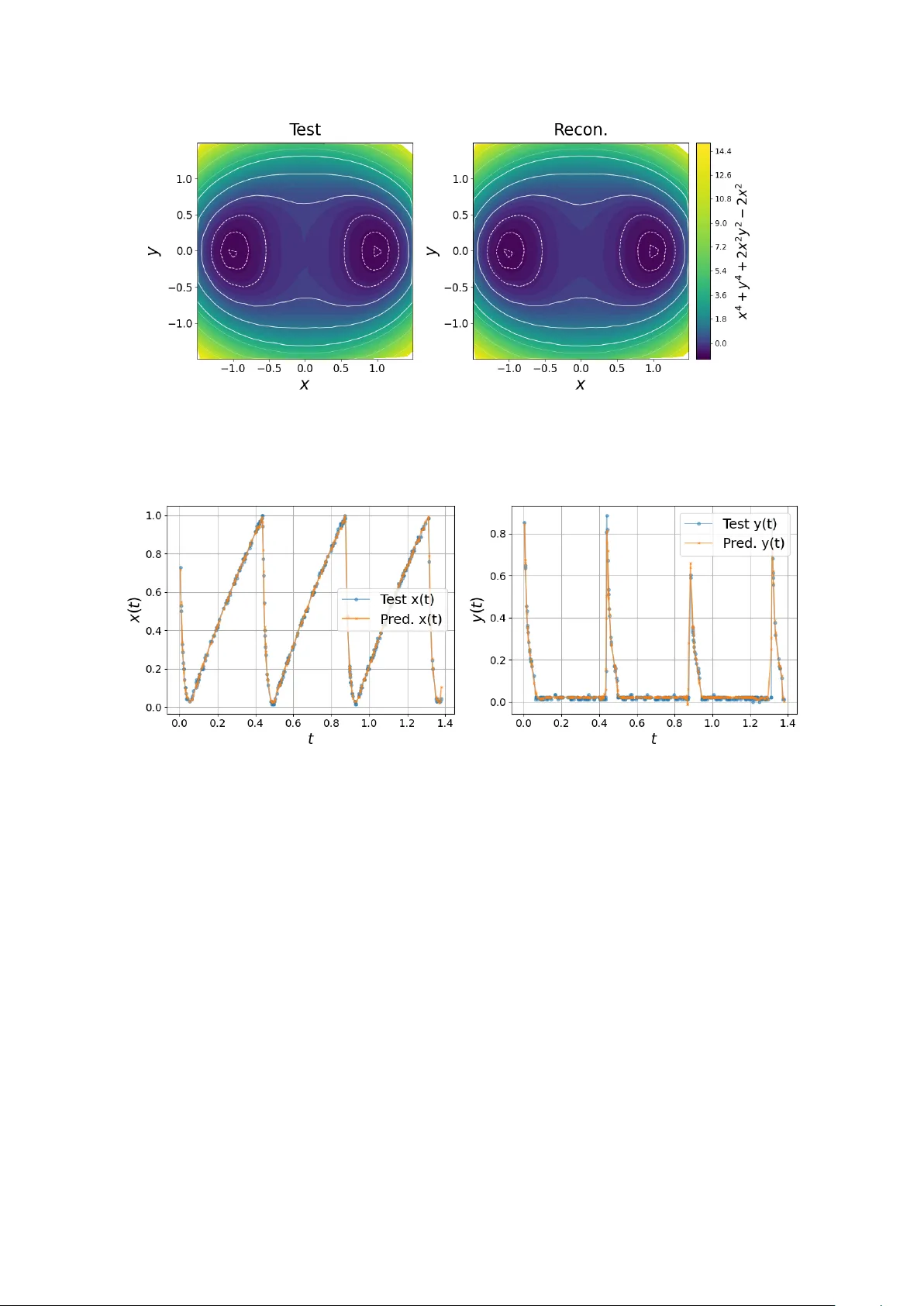
Leave a Comment