Evolutionary Discovery of Reinforcement Learning Algorithms via Large Language Models

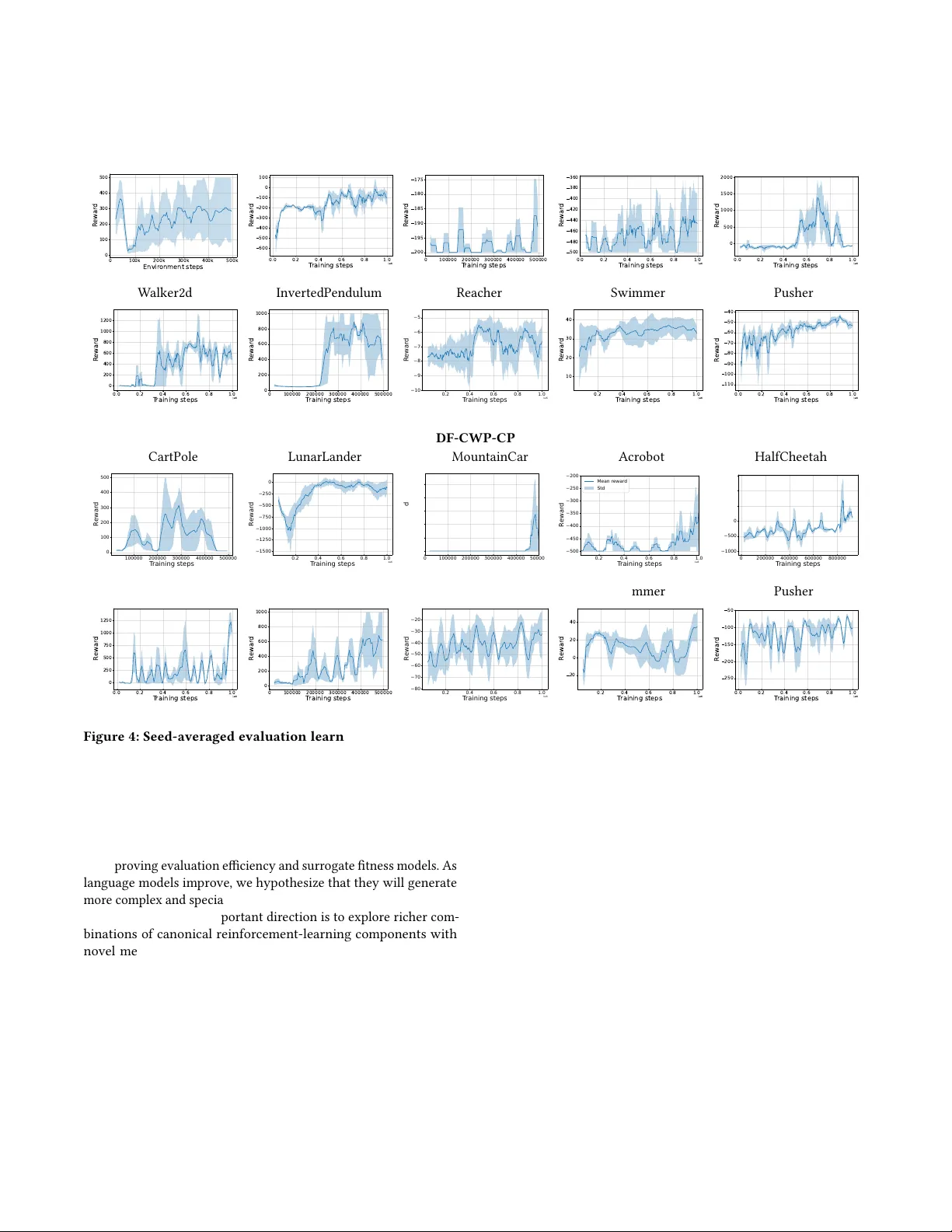
Evolutionary Discov er y of Reinforcement Learning Algorithms via Large Language Mo dels Alkis Sygkounas Machine Perception and Interaction Lab, Ör ebro University Sweden alkis.sygkounas@oru.se Amy Lout Machine Perception and Interaction Lab, Ör ebro University Sweden amy .lout@oru.se Andreas Persson Machine Perception and Interaction Lab, Ör ebro University Sweden andreas.persson@oru.se Abstract Reinforcement learning algorithms are dened by their learning up- date rules, which are typically hand-designed and xed. W e present an evolutionary framework for discovering reinforcement learning algorithms by searching directly over executable update rules that implement complete training procedures. The approach builds on REvolve, an evolutionary system that uses large language mo d- els as generative variation operators, and extends it fr om rewar d- function discovery to algorithm disco very . T o promote the emer- gence of nonstandard learning rules, the search excludes canonical mechanisms such as actor–critic structures, temporal-dierence losses, and value bootstrapping. Because reinfor cement learning algorithms are highly sensitive to internal scalar parameters, we introduce a post-evolution r enement stage in which a large lan- guage model proposes feasible hyperparameter ranges for each evolved update rule . Evaluated end-to-end by full training runs on multiple Gymnasium benchmarks, the discovered algorithms achieve competitive performance relative to established baselines, including SA C, PPO , DQN, and A2C. Ke ywords Reinforcement learning, ev olutionary algorithms, large language models, algorithm discovery 1 Introduction In reinforcement learning, the update rule determines how experi- ence is transformed into parameter updates, which directly shape the learning behavior . Although automated discov ery has been applied to some aspects of reinforcement le arning, such as archi- tecture design [ 27 , 31 , 36 ], hyperparameter tuning [ 5 , 26 , 35 ], and training-signal design [ 10 , 37 ], the up date rule typically remains xed. A small number of works have attempted to further elevate the discovery by exploring the learning of up date rules intrinsi- cally , either by optimizing dierentiable update functions [ 22 ], or by evolving structured loss expr essions [ 4 ]. Howev er , these meth- ods operate over restricted, parameterized repr esentations of the learning rule, such as dier entiable update networks or symbolic loss forms, and therefore cannot generate fundamentally dierent update rules expressed as executable training logic. As a result, the update rule remains one of the core components of reinforcement learning that has not yet been the subject of fully automated design. Searching over reinforcement-learning update rules is incom- patible with gradient-based or other locally guided optimization because the search space consists of discrete program structures implementing full training procedures, rather than continuous pa- rameters or dierentiable update modules. Even small changes to the update logic can induce qualitatively dierent learning dynam- ics, and reinforcement-learning algorithms are known to be highly sensitive to implementation details [ 6 , 12 ]. Hyperparameters that stabilize one up date rule often fail for another [ 25 ], prev enting eective local renement through small perturbations. As a result, each up date rule must b e treated as a distinct algorithm whose quality can only be assessed through complete training runs. Un- der these conditions, population-base d evolutionary methods are a natural t, since they compare candidate algorithms using end-to- end performance without requiring gradients or smooth objective structure [4, 13, 15]. Evolutionary algorithms and genetic programming have been applied to a wide range of machine-learning tasks, including neural network e volution, hyperparameter optimization, controller synthe- sis, and symbolic policy search [8, 13, 15]. A key practical require- ment in these settings is the ability to generate ospring that are both syntactically valid and executable, enabling ev olutionary oper- ators to explore the search space without producing predominantly invalid variants [ 4 ]. Reinforcement-learning update rules, however , violate this requirement because they are implemented as tightly coupled training proce dures rather than isolated obje ctive functions. As a r esult, e ven small structural code changes can break dependen- cies between components or invalidate required data ows, leading to failed or undened training behavior [ 6 , 12 , 25 ]. Consequently , unguided mutation and crossover are unlikely to r eliably produce functional update rules, underscoring the nee d for a guided mecha- nism that proposes coherent, executable modications to complete training logic. Recent work suggests that large language models (LLMs) can serve as such proposal mechanisms within evolutionary pipelines, enabling structured exploration of complex design spaces. In rein- forcement learning, this approach has been use d to optimize reward functions by generating rewar d implementations whose utility is assessed through training outcomes [ 9 , 20 ]. Related ideas have also been explored for program and code evolution within genetic programming frameworks [ 4 , 11 ], as well as for broader evolution- ary computation, such as population-based and quality-diversity search in neural architecture optimization [ 21 ]. However , across these lines of w ork, e volutionary search typically targets individual components of learning systems, while the reinforcement-learning update rule itself remains xed. In this work, we investigate ev olutionary search with large lan- guage models to discover novel reinforcement-learning algorithms by directly searching ov er learning update rules. Our approach builds on REvolve [ 9 ], which formulates re ward-function discov- ery as an evolutionary process using island populations [ 3 ] and Alkis Sygkounas, Amy Loutfi, and Andreas Persson language-model-based variation. W e apply the same evolutionary structure to a dierent sear ch space. Howe ver , instead of evolving r e- ward functions, w e evolv e learning update rules as e xecutable code under a xed policy architectur e, optimizer , and training congura- tion. In this setting, each candidate update rule denes a distinct reinforcement-learning algorithm. T o encourage the synthesis of noncanonical learning rules and to assess whether genuinely new update rules can emerge, we prohibit the use of standard mecha- nisms such as actor–critic decomposition [ 16 ], bootstrappe d value targets [ 33 ], and temporal-dierence error computation [ 33 ]. Each candidate algorithm is evaluated by full training on a xed set of environments, and selection is based on aggregated empirical performance. W e further extend REvolve with a post-evolution hy- perparameter optimization applied to top-performing algorithms to evaluate robustness and improv e stability under xed training bud- gets. An overview of the proposed method is illustrated in Figure 1. In summary , the main contributions of this pap er are as follows: • W e formulate reinforcement-learning algorithm discov ery as an evolutionary search process over executable learn- ing update rules, enabling the direct synthesis of complete learning algorithms. • W e extend REvolve to search in the update-rule space us- ing LLM-guided mutation and crossover , with explicit con- straints that exclude canonical RL mechanisms to promote the discovery of nonstandard algorithms. • W e empirically demonstrate that the proposed framework discovers new r einforcement-learning algorithms that achie ve competitive performance across multiple Gymnasium bench- marks after post-evolution hyperparameter optimization. 2 Related W ork Several lines of w ork have focused on automating components of reinforcement learning systems that are external to the learning update rule itself. This includes neural architecture search for rein- forcement learning agents [ 27 , 31 , 36 ], large-scale hyperparameter optimization frameworks targeting training stability and sample ef- ciency [ 13 , 35 ], and methods that automate the design of auxiliary objectives or training signals [ 10 , 14 ]. These approaches impro ve performance by modifying architectures, hyp erparameters, or train- ing signals, while the underlying update rule is typically held xed. Evolutionary and population-based methods provide a comple- mentary line of work that impro ves learning performance by op- erating over policies, parameters, or architectures within a xed training loop. This includes neuro-evolution approaches that evolve policy parameters or network structures [ 28 , 32 ], evolutionary strategies applied to p olicy optimization [ 15 , 30 ], population-based training methods that adapt hyp erparameters during learning [ 13 ], and evolutionary generation of environments and curricula [ 34 ]. More recently , large language models have been incorp orated into similar iterative optimization pipelines for reinforcement learn- ing and related domains, including generating or rening reward specications and training objectives [ 9 , 20 ], and proposing policy- level code or heuristics that are evaluated and selected through performance [11]. Gymnasium Environments Algorithm Population Per generation Post-evolution β i ∗ ¯ F k ( g ) ℒ f 1 ℒ f 2 ℒ f n ℒ ∗ Figure 1: Illustrative overview of the proposed method. A p op- ulation of candidate algorithms is iteratively evolved. In each generation (solid arrows), a large language model proposes coherent variants ( L 𝑓 1 , L 𝑓 2 , . . . , L 𝑓 𝑛 ), which are evaluated via training in Gymnasium environments to obtain tness scores ( ¯ 𝐹 ( 𝑔 ) 𝑘 ) that are subsequently used for sele ction and p opulation updates. Post-evolution (dashed arrows), a hyperparameter setting ( 𝛽 ★ 𝑖 ), selecte d via LLM-guided optimization, optimizes the resulting best update rule ( L ★ ), which is then advanced for nal evaluation. Collectively , existing approaches have explored automated and evolutionary optimization of architectures, hyperparameters, re- wards, environments, and policy parameters. They have addition- ally introduced language models as generators within such search processes. However , with the exception of work that learns or evolves update rules in restricted forms [ 2 , 4 , 22 ], these approaches treat the reinforcement learning update rule itself as xed. In con- trast, our work targets algorithm discovery at the level of the update rule, treating the executable learning logic as the object of e volu- tionary search. 3 Methodology For this work, we consider reinforcement learning problems de- ned by a Markov decision process M = (S , A , 𝑃 , 𝑟 ) . At interaction step 𝑡 , the agent observes 𝑠 𝑡 ∈ S , selects an action 𝑎 𝑡 ∈ A ac- cording to a policy 𝜋 𝜃 ( 𝑎 | 𝑠 ) and parameterized by 𝜃 , receives reward 𝑟 𝑡 , and transitions to 𝑠 𝑡 + 1 , producing experience tuples 𝑒 𝑡 = ( 𝑠 𝑡 , 𝑎 𝑡 , 𝑟 𝑡 , 𝑠 𝑡 + 1 , 𝑑 𝑡 ) . The accumulated experience is denoted D 𝑡 = { 𝑒 0 , . . . , 𝑒 𝑡 } . Hence, a reinforcement learning algorithm is de- ned by its learning update rule , where each candidate update rule 𝑓 species an executable training procedure whose cor e comp onent is a dierentiable loss function: L 𝑓 ( 𝜃 , 𝜉 𝑡 ; D 𝑡 ) , where 𝜃 denotes the policy parameters (including a xed architec- ture trunk and output head), and 𝜉 𝑡 denotes all auxiliary trainable components and internal state introduced by the up date rule (e.g., parameters of auxiliar y networks or target models) that are updated Evolutionary Discovery of Reinforcement Learning Algorithms via Large Language Models during training. The induced parameter updates are given by: Δ 𝜃 𝑡 = − 𝜂 𝑓 ∇ 𝜃 L 𝑓 ( 𝜃 𝑡 , 𝜉 𝑡 ; D 𝑡 ) , Δ 𝜉 𝑡 = − 𝜂 𝜉 𝑓 ∇ 𝜉 L 𝑓 ( 𝜃 𝑡 , 𝜉 𝑡 ; D 𝑡 ) , where 𝜂 𝑓 and 𝜂 𝜉 𝑓 are rule-specic update coecients. The resulting training dynamics are subsequently: 𝜃 𝑡 + 1 = 𝜃 𝑡 + Δ 𝜃 𝑡 , 𝜉 𝑡 + 1 = 𝜉 𝑡 + Δ 𝜉 𝑡 . The up date rule therefore denes the program-level mapping 𝑓 ( 𝜃 𝑡 , 𝜉 𝑡 , D 𝑡 ) : = Δ 𝜃 𝑡 . The search space F consists of all executable update rules of this form that induce valid parameter updates, i.e., 𝜃 𝑡 + Δ 𝜃 𝑡 ∈ Θ for all admissible ( 𝜃 𝑡 , 𝜉 𝑡 , D 𝑡 ) . Under a xed policy architecture, optimizer , and training loop, each distinct 𝑓 ∈ F denes a distinct reinforcement learning algorithm. 3.1 Training Performance and Fitness Each update rule 𝑓 ∈ F is evaluated by executing a complete reinforcement learning training run. For a xed environment M 𝑖 , let: T ( 𝑓 , M 𝑖 ) = { 𝑅 𝑖 ,𝑡 ( 𝑓 ) } 𝑇 𝑡 = 1 , denote the stochastic training-and-evaluation process that produces a sequence of evaluation returns by p eriodically evaluating the policy 𝜋 𝜃 𝑡 during training. Training is performed independently on a xed set of environments { M 𝑖 } 𝑁 𝑖 = 1 . For each environment, performance is summarize d by the maxi- mum evaluation return attained over the training horizon, MTS 𝑖 ( 𝑓 ) = max 𝑡 ≤ 𝑇 𝑅 𝑖 ,𝑡 ( 𝑓 ) , corresponding to the b est policy produced by the update rule during training. T o account for dierences in reward scale across environ- ments, these scores are normalized using environment-specic reference bounds 𝐿 𝑖 and 𝑈 𝑖 , ˜ 𝐹 𝑖 ( 𝑓 ) = MTS 𝑖 ( 𝑓 ) − 𝐿 𝑖 𝑈 𝑖 − 𝐿 𝑖 . The evolutionary tness is dened as the mean normalized perfor- mance across environments, 𝐹 ( 𝑓 ) = 1 𝑁 𝑁  𝑖 = 1 ˜ 𝐹 𝑖 ( 𝑓 ) . 3.2 Evolutionary Selection Mechanism The evolutionary process follows the same process as presented in REvolve [ 9 ]. At initialization, each island is populated with an independently sampled set of update rules. Let P ( 𝑔 ) 𝑘 denote the population of island 𝑘 at generation 𝑔 , with xed population size 𝑁 . At each generation, a total of 𝑀 new candidate update rules are generated across all islands, with variation applied independently within each island population. Let: ¯ 𝐹 ( 𝑔 ) 𝑘 = 1 𝑁  𝑓 ∈ P ( 𝑔 ) 𝑘 𝐹 ( 𝑓 ) , denote the mean tness of the current population of island 𝑘 . A newly generated candidate 𝑓 is accepted if: 𝐹 ( 𝑓 ) ≥ ¯ 𝐹 ( 𝑔 ) 𝑘 . Accepted candidates replace the lowest-tness members of P ( 𝑔 ) 𝑘 , keeping the population size constant. 3.3 V ariation Operators New candidates are generated using macro mutation and diversity- aware crossover , selected stochastically with probabilities 𝑝 and 1 − 𝑝 , respectively . In REvolve , micro mutations operate on short- reward expressions, where local edits can pr oduce graded behav- ioral changes. For update rules, early generations contain low- performing algorithms, whose deciencies are structural rather than local. Hence, minor token edits do not lead to meaningful im- provements and often destabilize training. Macro mutation, on the other hand, rewrites exactly one semantically coherent component of the update rule in a single step, enabling substantial changes to the learning logic [17, 29, 32]. Crossover combines two parent update rules. If parents are se- lected purely by tness, crossover frequently recombines a rule with a near duplicate created in a recent mutation, yielding o- spring that dier only trivially from their par ents and collapsing population diversity [ 19 ]. T o avoid this, par ent selection incorpo- rates structural dissimilarity measured via normalized Levenshtein distance [18]. Parent 1 is drawn from the current island population P ( 𝑔 ) 𝑘 using a tness-proportional softmax: 𝑃 ( 𝑓 1 ) = exp ( 𝜏 𝐹 ( 𝑓 1 ) ) Í 𝑓 ∈ P ( 𝑔 ) 𝑘 exp ( 𝜏 𝐹 ( 𝑓 ) ) , 𝜏 > 0 . The tness values are normalized such that 𝐹 ( 𝑓 ) ∈ [ 0 , 1 ] , where the structural dissimilarity measure 𝑑 lev ( 𝑓 1 , 𝑓 2 ) is dened as a nor- malized Levenshtein distance taking values in [ 0 , 1 ] . Conditional on 𝑓 1 , Parent 2 is sampled accor ding to the combined score: 𝑆 ( 𝑓 2 | 𝑓 1 ) = 𝛼 𝐹 ( 𝑓 2 ) + ( 1 − 𝛼 ) 𝑑 lev ( 𝑓 1 , 𝑓 2 ) , where 𝑑 lev ( 𝑓 1 , 𝑓 2 ) is computed b etween the source-code representa- tions of the corresponding compute_loss functions, and 𝛼 ∈ [ 0 , 1 ] balances tness and structural dissimilarity . The resulting sampling distribution is consequently: 𝑃 ( 𝑓 2 | 𝑓 1 ) = exp ( 𝜏 𝑆 ( 𝑓 2 | 𝑓 1 ) ) Í 𝑓 ∈ P ( 𝑔 ) 𝑘 exp ( 𝜏 𝑆 ( 𝑓 | 𝑓 1 ) ) . Higher tness increases selection probability , but structurally similar candidates are penalized unless they oer clear performance advantages. This discourages cr ossover between a parent and its mi- nor variants and promotes recombination b etween high-performing yet distinct update rules. The variation operator then selects macro mutation or crossover with pr obabilities 𝑝 and 1 − 𝑝 , respectively , and applies the selected operator to generate a new candidate. 3.4 LLM-Based Generative Operator Macro mutation and crosso ver are implemented through a condi- tional generative operator: 𝑓 ′ ∼ 𝑞 𝜙 ( 𝑓 1 , 𝑓 2 , op , R , E ) , realized using a large language model. The operator takes as input the parent update rules ( 𝑓 1 , 𝑓 2 ) , the selected variation instruction Alkis Sygkounas, Amy Loutfi, and Andreas Persson op ∈ { macro , crossover } , summary training metrics R , and the envi- ronment interface E specifying obser vation and action spaces. The output 𝑓 ′ is represented as an executable implementation of an up- date rule, including the denition of the loss L 𝑓 ′ and any auxiliary state updates for 𝜉 . During evolutionary variation, the generation process is constrained to forbid explicit instantiation of canoni- cal reinforcement learning mechanisms, including actor–critic de- composition, bootstrapp ed value targets, and temporal-dierence updates. These constraints are applied only during evolutionary search. 3.5 Post-Evolution: LLM-Guided Hyperparameter Optimization (LLM-HPO ) REvolve terminates after evolutionary search without additional tuning of selecte d individuals. For the evolution of update rules, this is insucient as reinforcement learning algorithms are highly sensitive to internal scalar parameters, and a xed parameterization can severely underestimate the quality of an update rule [ 6 , 12 ]. Instead, we let each evolv ed update rule ˆ 𝑓 dene a family of algo- rithms parameterized by 𝛽 ∈ R 𝑑 , wher e 𝛽 collects all internal scalar coecients of the rule. After evolutionary convergence, w e optimize the top- 𝐾 update rules { ˆ 𝑓 1 , . . . , ˆ 𝑓 𝐾 } by appro ximating: max 𝛽 ∈ B ˆ 𝑓 𝐹  𝑓 𝛽  , where 𝐹 ( ·) denotes the aggregated tness across e valuation envi- ronments and B ˆ 𝑓 ⊂ R 𝑑 is a rule-specic feasible parameter region. Exhaustive search ov er B ˆ 𝑓 is infeasible when tness must be eval- uated through full training runs on multiple environments. For each ˆ 𝑓 , the language model is provided with the full up date- rule implementation together with the sp ecications of the evalua- tion environments, and returns bounded numeric intervals: B ˆ 𝑓 = 𝑑 Ö 𝑗 = 1 [ ℓ 𝑗 , 𝑢 𝑗 ] , one for each internal scalar parameter 𝛽 𝑗 . These intervals dene an LLM-guided search region that restricts exploration to numerically plausible ranges conditioned on both the algorithm structure and the environment suite. A sweep then uniformly samples parameter vectors 𝛽 from B ˆ 𝑓 , instantiates the corresponding update rule 𝑓 𝛽 , and evaluates its tness separately for each environment using the same evaluation protocol as during evolution. For each ˆ 𝑓 𝑖 , the parameter vector: 𝛽 ★ 𝑖 = arg max 𝛽 𝐹  𝑓 𝛽  , observed during this sampling-based optimization is retained, yield- ing the nal rened algorithm 𝑓 𝛽 ★ 𝑖 . The policy architecture, opti- mizer , rollout procedure, and training loop remain xed throughout this stage. 4 Experiments For experiments, we perform evolutionary search using two large language models as generative operators, namely GPT -5.2 and Claude 4.5 Opus. For each language model, we conduct two in- dependent evolutionary runs with dierent ev olutionary random seeds. Each run is executed for 10 generations, and at ev ery genera- tion, each island produces 24 new candidate update rules. V ariation operators ar e applied with xed probabilities 𝑝 macro = 0 . 65 and 𝑝 cross = 0 . 35 , while div ersity-aware crosso ver is regulated by a Levenshtein distance weight 𝛼 = 0 . 5 . Candidate update rules are evaluated across a xed set of envi- ronments: CartPole-v1, MountainCar-v0, Acrobot-v1, LunarLander- v3, and HalfCheetah-v5. CartPole-v1 ser ves as a minimal control task for verifying basic learning functionality . MountainCar-v0 and Acr obot-v1 feature sparse rewards in discrete action spaces. LunarLander-v3 combines discrete control with shaped rewards and more complex dynamics. HalfCheetah-v5 represents a high- dimensional continuous-control task with dense rewards. T ogether , this suite spans discrete and continuous action spaces as well as sparse and dense reward regimes, and consists of environments with established reward scales that support consistent tness nor- malization and comparison across tasks [ 1 , 7 , 23 , 24 ]. Figure 2 pro- vides representative visualizations of the Gymnasium benchmark environments used for training and evaluation. Each candidate update rule is evaluated by training it on each of the ve environments using 𝑆 = 5 independent random seeds per environment, yielding 25 training runs per candidate. For a given environment, p erformance is summarized as the average across seeds of the maximum evaluation (best checkpoint model) return achieved during training. These environment-level scores are then normalized to the unit interval using environment-specic reward bounds as described in Section 3.2, and aggregated across environments to obtain the nal scalar tness used for ev olution- ary sele ction. Additional details on environment choice and tness computation are provided in Appendix A. All evolutionary experi- ments were conducted on four A100 GP Us with 40 GB of memory each. Under this setup, a single evolutionary generation required approximately 30 hours of wall-clock time. 5 Results Figure 3 shows the e volutionary progress obtained with GPT -5.2 and Claude 4.5 Opus. For each language model, r esults ar e reported for two independent evolutionary runs with dierent random seeds. At each generation, the plotted value corresponds to the best- performing up date rule in the population at that generation, as measured by the aggregated tness dened in Se ction 3.2. Both language models exhibit a monotonic increase in maximum t- ness across generations for both evolutionary seeds, as seen in Figure 3. GPT -5.2 consistently attains higher tness values than Claude 4.5 Opus throughout evolution, with nal-generation tness in the range [ 0 . 65 , 0 . 69 ] across seeds, compared to [ 0 . 37 , 0 . 47 ] for Claude 4.5 Opus. The shaded regions denote the min–max range across the two evolutionary seeds, indicating moderate variability without qualitative divergence between runs. Final algorithm selection and evaluation. At the end of ev olution- ary search, we select the highest-tness update rule from the nal generation of each evolutionary seed. For GPT -5.2, this yields two distinct algorithms corresponding to the two indep endent evolution- ary runs. Update rules evolved using Claude 4.5 Opus consistently Evolutionary Discovery of Reinforcement Learning Algorithms via Large Language Models (a) CartPole (b) LunarLander (c) MountainCar (d) Acrobot (e) HalfChe etah (f ) W alker2d (g) InvertedPendulum (h) Reacher (i) Swimmer ( j) Pusher Figure 2: Representative Gymnasium environments used for training (top row ) and evaluation ( bottom row). 0 1 2 3 4 5 6 7 8 9 Generation 0.25 0.30 0.35 0.40 0.45 0.50 0.55 0.60 0.65 0.70 F itness GPT -5.2 Claude Opus 4.5 Figure 3: Evolution of maximum population tness across generations for GPT -5.2 and Claude 4.5 Opus. Curves show the mean across two evolutionary seeds, with shaded regions indicating the standard deviation across seeds. achieved substantially lower tness and did not pr oduce competi- tive candidates in the nal generation, and are ther efore excluded from further analysis. Each selected algorithm is evaluated on the full suite of ten envi- ronments shown in Figure 2, including both the ve environments used during evolutionary search and ve additional environments not seen during tness optimization. For each environment, we report the best performance achieved after post-evolution hyper- parameter optimization, following the evaluation protocol dened in Se ction 3.2. This procedure reects the maximal performance attainable by a given update rule under a xed training budget. The two highest-performing algorithms identied by this process are coined Condence-Guided For ward Policy Distillation (CG-FPD) and Dierentiable Forward Condence- W eighted Planning with Controllability Prior (DF-CWP-CP) . At a high level, CG-FPD trains a policy by distilling short-horizon plans from a learned latent dynamics model, using planning solely as a supervise d teacher signal. In contrast, DF-CWP-CP optimizes the policy via dierentiable short-horizon world-model rollouts that incorporate condence-weighted desirability and controllability objectives. Both algorithms avoid value functions, p olicy gradients, and Bellman-style updates, and instead r ely on planning-derived learning signals. Detailed descriptions of their internal mechanisms are provided in Appendix B. Generalization across environments. Evolutionary tness is com- puted on only ve training environments, which may lead to over- tting. T o assess generalization, we evaluate the two selected algo- rithms, CG-FPD and DF-CWP-CP , on ten environments (Figure 2), including the ve training and ve unse en ones. All evaluations follow the same protocol as during ev olution, and results report the best performance after post-evolution hyperparameter tuning. W e compare against PPO , A2C, DQN, and SAC baselines using an identical 256 × 256 MLP policy architecture ( Appendix A.1). T able 1 shows the maximum evaluation return per environment. Training stability . Beyond nal performance, we analyze learn- ing dynamics to assess stability . Figure 4 shows seed-averaged evaluation curves for the two best evolv ed algorithms. In most environments, both reach high performance within the training budget, but learning is often non-monotonic and not consistently maintained at the end. Despite this, the best checkp oints (T able 1) correspond to policies that solve or perform competitively on the tasks. Alkis Sygkounas, Amy Loutfi, and Andreas Persson Environment PPO A2C DQN SA C CG-FPD DF-CWP-CP CartPole 500 . 0 ± 0 . 0 500 . 0 ± 0 . 0 500 . 0 ± 0 . 0 – 500 . 0 ± 0 . 0 500 . 0 ± 0 . 0 LunarLander 246 . 60 ± 30 . 9 246 . 60 ± 13 . 4 250 . 10 ± 4 . 10 – 241 . 20 ± 11 . 0 260 . 60 ± 19 . 12 MountainCar − 128 . 12 ± 44 . 64 − 134 . 20 ± 8 . 70 − 147 . 80 ± 40 . 40 – − 105 . 80 ± 10 . 51 − 108 . 67 ± 7 . 34 Acrobot − 63 . 5 ± 0 . 8 − 213 . 6 ± 202 . 5 − 61 . 90 ± 0 . 10 – − 90 . 6 ± 5 . 86 − 78 . 67 ± 8 . 72 HalfChe etah 1579 . 13 ± 643 . 80 795 . 91 ± 147 . 70 – 4988 . 5 ± 2667 . 70 2407 . 88 ± 311 . 90 2103 . 80 ± 246 . 70 Reacher − 3 . 15 ± 0 . 14 − 6 . 48 ± 0 . 57 – − 2 . 05 ± 0 . 19 − 2 . 67 ± 0 . 15 − 5 . 43 ± 0 . 44 Swimmer 95 . 0 ± 29 . 20 49 . 08 ± 1 . 07 – 87 . 84 ± 23 . 50 247 . 54 ± 35 . 53 219 . 82 ± 32 . 33 Inverted Pendulum 1000 . 0 ± 0 . 0 1000 . 0 ± 0 . 0 – 1000 . 0 ± 0 . 0 1000 . 0 ± 0 . 0 1000 . 0 ± 0 . 0 W alker2d 3163 . 20 ± 397 . 20 801 . 50 ± 291 . 10 – 4595 . 30 ± 252 . 20 1603 . 80 ± 146 . 70 1297 . 63 ± 62 . 77 Pusher − 25 . 50 ± 0 . 32 − 32 . 41 ± 0 . 81 – − 25 . 50 ± 0 . 32 − 27 . 23 ± 0 . 86 − 39 . 88 ± 0 . 92 T able 1: Mean ± standard deviation of the maximum evaluation return p er environment. Each algorithm is trained with ve seeds; for each se ed, the checkpoint with the highest evaluation return is evaluated over 100 episodes, and results report the mean and standard deviation across seeds. Dashes (– ) indicate inapplicability ( e.g., SA C for discrete environments, DQN for continuous control). PPO and A2C support both action typ es and are evaluated alongside the evolved methods (CG-FPD and DF-CWP-CP) on all compatible environments. 5.1 Ablation Studies Sensitivity to the Levenshtein weight 𝛼 . W e study the eect of the Levenshtein r egularization weight 𝛼 (Eq. 3.3) on evolutionary dynamics by comparing 𝛼 = 0 (no structural regularization) and 𝛼 = 1 (full regularization). A s shown in Figure 5, enforcing struc- tural similarity improves both convergence speed and nal tness relative to unconstrained mutation, indicating that similarity-aware variation stabilizes sear ch in update-rule space. Across evolutionary runs, 𝛼 = 0 and 𝛼 = 1 reach maximum tness values of approx- imately 0 . 50 and 0 . 56 , respectively . In contrast, the intermediate setting 𝛼 = 0 . 5 , used for all main experiments reported in Figure 3, consistently attains higher nal tness in the range [ 0 . 65 , 0 . 69 ] across both evolutionary seeds. This pattern indicates that partial structural regularization yields a mor e eective balance between preserving functional code structure and enabling exploratory vari- ation. 0 1 2 3 4 5 6 7 8 9 Generation 0.400 0.425 0.450 0.475 0.500 0.525 0.550 F itness α = 0 α = 1 Figure 5: Ablation of the Levenshtein regularization weight 𝛼 in the evolutionary objective (Eq. 3.3). Cur ves show best population tness per generation for 𝛼 = 0 and 𝛼 = 1 , aver- aged across evolutionary seeds. T erminal value bootstrap. W e ablate CG-FPD by adding a ter- minal value estimate to its planner . Specically , w e introduce a value head 𝑉 ( ℎ ) trained with one-step temporal-dierence learning (TD(0)), i.e., regression to the immediate reward plus the estimated value of the ne xt state, on the same robust-normalized re ward used by CG-FPD . Its output is used only as a bounded terminal bonus in the planner score, and all other policy components and settings are identical to the baseline. Acr oss all tested environments, adding a terminal-value bo otstrap reduces peak p erformance relative to CG-FPD but consistently lowers variance across seeds, indicating improved stability . This suggests that CG-FPD is not limited by missing long-horizon return estimates; rather , introducing a learned value signal biases planning and degrades peak p erformance, even when used only as a bounded terminal bonus. The stability gains imply that value estimates act as a regularizer for planning, at the cost of restricting high-performing behavior . Environment CG-FPD ( baseline) CG-FPD + value bootstrap MountainCar-v0 -105.80 ± 10.51 -122.12 ± 7.32 LunarLander-v3 241.20 ± 11.00 194.68 ± 7.04 Reacher -2.67 ± 0.15 -3.27 ± 0.11 T able 2: Ablation of terminal value b ootstrap added to CG- FPD. Results report mean ± standard deviation of peak eval- uation return over random seeds. 6 Limitation & Future W ork The framework is computationally expensive, since each candidate update rule must be evaluated through full reinfor cement-learning training across multiple environments and random se eds, which restricts the scale of evolutionary search. In the curr ent setting, the discovered algorithms arise from no vel recombinations of existing reinforcement-learning mechanisms rather than from fundamen- tally new update forms, reecting both the structure of the search space and the representational limits of the language model used to generate candidate rules. Evolutionary Discovery of Reinforcement Learning Algorithms via Large Language Models CG-FPD CartPole LunarLander MountainCar Acrobot HalfCheetah 0 100k 200k 300k 400k 500k Envir onment steps 0 100 200 300 400 500 R ewar d 0.0 0.2 0.4 0.6 0.8 1.0 T raining steps 1e6 600 500 400 300 200 100 0 100 R ewar d 0 100000 200000 300000 400000 500000 T raining steps 200 195 190 185 180 175 R ewar d 0.0 0.2 0.4 0.6 0.8 1.0 T raining steps 1e6 500 480 460 440 420 400 380 360 R ewar d 0.0 0.2 0.4 0.6 0.8 1.0 T raining steps 1e6 0 500 1000 1500 2000 R ewar d W alker2d InvertedPendulum Reacher Swimmer Pusher 0.0 0.2 0.4 0.6 0.8 1.0 T raining steps 1e6 0 200 400 600 800 1000 1200 R ewar d 0 100000 200000 300000 400000 500000 T raining steps 0 200 400 600 800 1000 R ewar d 0.2 0.4 0.6 0.8 1.0 T raining steps 1e6 −10 −9 −8 −7 −6 −5 Rewar d 0.2 0.4 0.6 0.8 1.0 T raining steps 1e6 10 20 30 40 R ewar d 0.0 0.2 0.4 0.6 0.8 1.0 T raining steps 1e6 110 100 90 80 70 60 50 40 R ewar d DF-CWP-CP CartPole LunarLander MountainCar Acrobot HalfCheetah 100000 200000 300000 400000 500000 T raining steps 0 100 200 300 400 500 Rewar d 0.2 0.4 0.6 0.8 1.0 T raining steps 1e6 −1500 −1250 −1000 −750 −500 −250 0 Rewar d 0 100000 200000 300000 400000 500000 T raining steps −200 −195 −190 −185 −180 −175 Rewar d 0.2 0.4 0.6 0.8 1.0 T raining steps 1e6 −500 −450 −400 −350 −300 −250 −200 Rewar d Mean reward Std 0 200000 400000 600000 800000 T raining steps −1000 −500 0 500 1000 1500 Rewar d W alker2d InvertedPendulum Reacher Swimmer Pusher 0.0 0.2 0.4 0.6 0.8 1.0 T raining steps 1e6 0 250 500 750 1000 1250 R ewar d 0 100000 200000 300000 400000 500000 T raining steps 0 200 400 600 800 1000 R ewar d 0.2 0.4 0.6 0.8 1.0 T raining steps 1e6 −80 −70 −60 −50 −40 −30 −20 Rewar d 0.2 0.4 0.6 0.8 1.0 T raining steps 1e6 20 0 20 40 R ewar d 0.0 0.2 0.4 0.6 0.8 1.0 T raining steps 1e6 250 200 150 100 50 R ewar d Figure 4: Seed-averaged evaluation learning curves for the two evolved algorithms across ten environments. T op: CG-FPD. Bottom: DF-CWP-CP. Cur ves show evaluation return smoothed with a moving average; shaded regions indicate one standard deviation across se eds. CartPole, InvertedPendulum, and MountainCar are trained for 500k steps, while all other environments are trained for 1M steps. Peak evaluation returns obser ved at the p er-seed level are attenuated in the seed-averaged smoothed curves. Future work will, therefore, focus on scaling ev olutionary search by improving evaluation eciency and surrogate tness models. A s language models improve , we hypothesize that they will generate more complex and specialized update rules, potentially conditioned on task structure. An important direction is to explore richer com- binations of canonical reinforcement-learning comp onents with novel mechanisms generated by language mo dels, and to study task-adaptive algorithm discovery . 7 Conclusion In this work, we pr esented an evolutionary framework for discov- ering reinforcement-learning algorithms by searching directly o ver executable update rules. Building on REvolve , candidate training procedures are generated by large language models and selected based on empirical performance across environments, shifting op- timization from architectures and hyperparameters to the learning procedure itself. The evolved update rules achieve competitive performance across a diverse benchmark suite without relying on predened actor-critic or temporal-dierence structures. These results demonstrate that update-rule space is a viable target for evolutionary search and that language models can serve as eective generative operators over algorithmic code for automated reinforcement-learning algorithm discovery . Acknowledgments This work is supported by Knut and Alice W allenb erg Foundation via the W allenberg AI A utonomous Sensors Systems and the W allen- berg Scholars Grant. W e also acknowledge the National Academic Alkis Sygkounas, Amy Loutfi, and Andreas Persson Infrastructure for Supercomputing in Sweden (NAISS), partially funded by the Swedish Research Council through grant agreement no. 2022-06725, for awarding this project access to the LUMI super- computer , owned by the EuroHPC Joint Undertaking and hosted by CSC (Finland) and the LUMI consortium. References [1] Hazim Alzorgan and Abolfazl Razi. 2025. Monte Carlo Beam Search for Actor- Critic Reinforcement Learning in Continuous Control. arXiv preprint (2025). https://arxiv .org/abs/2505.09029v1 Reports HalfCheetah-v4 returns around 12750 for strong baselines. [2] Marcin Andrychowicz, Misha Denil, Sergio Gomez, Matthew W Homan, David Pfau, T om Schaul, Brendan Shillingford, and Nando De Freitas. 2016. Learning to learn by gradient descent by gradient descent. Advances in neural information processing systems 29 (2016). [3] Erick Cantú-Paz et al . 1998. A survey of parallel genetic algorithms. Calculateurs paralleles, reseaux et systems repartis 10, 2 (1998), 141–171. [4] John D. Co-Re yes, Xue Bin Peng, Sergey Levine, Pieter Abbeel, and John Schul- man. 2021. Evolving Reinfor cement Learning Algorithms. In 9th International Conference on Learning Representations (ICLR) . https://openreview .net/forum? id=9XlAMdLMrB [5] Theresa Eimer , Marius Lindauer, and Roberta Raileanu. 2023. Hyp erparameters in reinforcement learning and how to tune them. In International conference on machine learning . PMLR, 9104–9149. [6] Logan Engstrom, Andrew Ilyas, Shibani Santurkar , Dimitris Tsipras, Firdaus Janoos, Larry Rudolph, and Aleksander Madry . 2020. Implementation mat- ters in deep p olicy gradients: A case study on ppo and trpo. arXiv preprint arXiv:2005.12729 (2020). [7] Farama Foundation. 2023. Gymnasium: A Standard API for Reinforcement Learning. https://gymnasium.farama.org/. Gymnasium documentation. [8] Jörg KH Franke, Gregor Köhler , No or Awad, and Frank Hutter . 2019. Neural architecture evolution in deep reinforcement learning for continuous control. arXiv preprint arXiv:1910.12824 (2019). [9] Rishi Hazra, Alkis Sygkounas, Andreas Persson, Amy Lout, and Pedro Zuid- berg Dos Martires. 2025. REvolve: Reward Evolution with Large Language Models using Human Feedback. In The Thirteenth International Conference on Learning Representations . https://op enreview .net/forum?id=cJP UpL8mOw [10] T airan He, Y uge Zhang, Kan Ren, Minghuan Liu, Che W ang, W einan Zhang, Y uqing Y ang, and Dongsheng Li. 2022. Reinforcement learning with automated auxiliary loss search. Advances in neural information processing systems 35 (2022), 1820–1834. [11] Erik Hemb erg, Stephen Moskal, and Una-May O’Reilly . 2024. Evolving code with a large language model. Genetic Programming and Evolvable Machines 25, 2 (2024), 21. [12] Peter Henderson, Riashat Islam, Philip Bachman, Joelle Pineau, Doina Precup, and David Meger . 2018. Deep reinforcement learning that matters. In Proceedings of the AAAI conference on articial intelligence , V ol. 32. [13] Max Jaderberg, V alentin Dalibard, Simon Osindero, W ojciech M Czarnecki, Je Donahue, Ali Razavi, Oriol Vinyals, Tim Green, Iain Dunning, Karen Si- monyan, et al . 2017. Population based training of neural networks. arXiv preprint arXiv:1711.09846 (2017). [14] Max Jaderberg, V olodymyr Mnih, W ojciech Marian Czarnecki, T om Schaul, Jo el Z Leibo, David Silver , and Koray Kavukcuoglu. 2016. Reinforcement learning with unsupervised auxiliar y tasks. arXiv preprint arXiv:1611.05397 (2016). [15] Shauharda Khadka and Kagan T umer . 2018. Evolution-guided policy gradient in reinforcement learning. Advances in Neural Information Processing Systems 31 (2018). [16] Vijay Konda and John Tsitsiklis. 1999. Actor-critic algorithms. Advances in neural information processing systems 12 (1999). [17] John R. Koza. 1992. Genetic Programming: On the Programming of Computers by Means of Natural Selection . MIT Press, Cambridge, MA, USA. [18] VI Lcvenshtcin. 1966. Binar y coors capable or ‘correcting deletions, insertions, and reversals. In Soviet physics-doklady , V ol. 10. [19] Joel Lehman and Kenneth O Stanley . 2011. Evolving a div ersity of virtual crea- tures through nov elty search and local competition. In Proceedings of the 13th annual conference on Genetic and evolutionary computation . 211–218. [20] Y echeng Jason Ma, William Liang, Guanzhi W ang, De- An Huang, Osbert Bastani, Dinesh Jayaraman, Yuke Zhu, Linxi Fan, and Anima Anandkumar . 2024. Eureka: Human-Level Re ward Design via Coding Large Language Mo dels. In The T welfth International Conference on Learning Representations . https://openreview .net/ forum?id=IEduRUO55F [21] Muhammad Umair Nasir , Sam Earle, Julian T ogelius, Steven James, and Christo- pher Cleghorn. 2024. Llmatic: neural architecture search via large language models and quality diversity optimization. In procee dings of the Genetic and Evolutionary Computation Conference . 1110–1118. [22] Junhyuk Oh, Rishabh Agarwal, Kelvin Xu, Dale Schuurmans, Quoc V . Le, and Mohammad Norouzi. 2020. Discovering Reinforcement Learning Al- gorithms. In Advances in Neural Information Processing Systems (NeurIPS) , V ol. 33. 1060–1070. https://papers.nips.cc/paper_les/paper/2020/hash/ a322852ce0df73e204b7df bce9c8cfd0- Abstract.html [23] OpenAI Gym. 2016. Leaderboard Solved Denitions (LunarLander-v2). https: //github.com/openai/gym/wiki/Leaderboard. Lists average reward 200 as solved for LunarLander . [24] OpenAI Gym. 2016. MountainCar-v0. https://github.com/openai/gym/wiki/ mountaincar- v0. OpenAI Gym Wiki. [25] Andrew Patterson, Samuel Neumann, Martha White, and Adam White. 2024. Empirical design in reinfor cement learning. Journal of Machine Learning Research 25, 318 (2024), 1–63. [26] Supratik Paul, Vitaly Kurin, and Shimon Whiteson. 2019. Fast ecient hyper- parameter tuning for policy gradient methods. Advances in Neural Information Processing Systems 32 (2019). [27] Hieu Pham, Melody Guan, Barret Zoph, Quoc Le, and Je Dean. 2018. Ecient neural architecture search via parameters sharing. In International conference on machine learning . PMLR, 4095–4104. [28] Esteban Real, Alok Aggarwal, Y anping Huang, and Quoc V Le. 2019. Regularized evolution for image classier architecture search. In Procee dings of the aaai conference on articial intelligence , V ol. 33. 4780–4789. [29] Esteban Real, Sherry Moore, Andrew Selle, Saurabh Saxena, Y utaka Leon Sue- matsu, Jie T an, Quoc V Le, and Alexey Kurakin. 2017. Large-scale evolution of image classiers. In International conference on machine learning . PMLR, 2902– 2911. [30] Tim Salimans, Jonathan Ho, Xi Chen, Szymon Sidor, and Ilya Sutskever . 2017. Evolution strategies as a scalable alternative to r einforcement learning. arXiv preprint arXiv:1703.03864 (2017). [31] Rei Sato, Jun Sakuma, and Y ouhei Akimoto . 2021. Advantagenas: Ecient neural architecture search with credit assignment. In Proceedings of the AAAI Conference on Articial Intelligence , V ol. 35. 9489–9496. [32] Kenneth O Stanley and Risto Miikkulainen. 2002. Ev olving neural networks through augmenting topologies. Evolutionary computation 10, 2 (2002), 99–127. [33] Richard S Sutton, David McAllester , Satinder Singh, and Yishay Mansour . 1999. Policy gradient methods for reinforcement learning with function approximation. Advances in neural information processing systems 12 (1999). [34] Rui W ang, Joel Lehman, Je Clune, and Kenneth O Stanley . 2019. Paired open- ended trailblazer (poet): Endlessly generating increasingly complex and diverse learning environments and their solutions. arXiv preprint (2019). [35] Zhongwen Xu, Hado P van Hasselt, and David Silver . 2018. Meta-gradient reinforcement learning. Advances in neural information processing systems 31 (2018). [36] Barret Zoph and Quoc V . Le. 2017. Neural Architecture Search with Reinforce- ment Learning. In 5th International Conference on Learning Representations (ICLR) . https://openreview .net/forum?id=r1Ue8Hcxg Oral Presentation. [37] Haosheng Zou, T ongzheng Ren, Dong Y an, Hang Su, and Jun Zhu. 2021. Learning task-distribution reward shaping with meta-learning. In Proceedings of the AAAI Conference on A rticial Intelligence , V ol. 35. 11210–11218. Evolutionary Discovery of Reinforcement Learning Algorithms via Large Language Models Appendix O verview This appendix is organized as follows. App endix A provides detailed environmental specications, reward denitions, and tness nor- malization. Appendix B describ es the two best-evolved algorithms, CG-FPD and DF-CWP-CP, including their internal mechanisms, and presents the terminal-value bootstrap ablation for CG-FPD and its implementation details. Appendix C reports the prompts used for the models. A Environment Details A.1 Fair Comparison and Fixed Policy Trunk T o isolate the eect of the learning update rule, we control rep- resentational capacity and optimization across all methods. Our PPO and SA C baselines use the standard MLP policy ar chitecture with two 256-unit hidden layers, and we adopt the same policy trunk and action head dimensions for all discovered algorithms. Concretely , the policy network is xed to a two-layer 256 × 256 T anh MLP with a linear output head, and is trained with the same optimizer ( Adam, lr = 3 × 10 − 4 ). In the algorithm-discov ery setting, candidate metho ds are therefore constrained to mo dify only the internal learning logic (e.g., the loss and auxiliary objectives) while keeping the policy parameterization and optimizer identical. This design ensures that performance dierences are attributable to the learned update rule rather than to netw ork size, architecture choice, or optimizer tuning. All discovered algorithms and baselines are evaluated every 5000 steps. Environment State Dim. Action Space Action T ype CartPole-v1 4 { 0 , 1 } Discrete MountainCar-v0 2 { 0 , 1 , 2 } Discrete LunarLander-v3 8 { 0 , 1 , 2 , 3 } Discrete Acrobot-v1 6 { 0 , 1 , 2 } Discrete InvertedPendulum-v4 4 R 1 Continuous HalfCheetah-v5 17 R 6 Continuous Hopper-v4 11 R 3 Continuous W alker2d-v4 17 R 6 Continuous Reacher-v4 11 R 2 Continuous Swimmer-v4 8 R 2 Continuous T able 3: Obser vation dimensionality and action space char- acteristics of the Gymnasium environments. A.2 Fitness Computation and Normalization This section describes how scalar tness values are computed from raw evaluation rewar ds during evolutionary search. Per-seed evaluation. For a xed update rule and environment, training is executed independently across multiple random seeds. During training, evaluation episodes are periodically run and the resulting episodic returns are logged. For each seed 𝑠 , we record the maximum evaluation return achiev ed during training, 𝑅 ( 𝑠 ) max = max 𝑡 ≤ 𝑇 𝑅 ( 𝑠 ) 𝑡 , where 𝑅 ( 𝑠 ) 𝑡 denotes the evaluation return at evaluation step 𝑡 . Environment Reward CartPole-v1 + 1 per timestep the pole remains upright. MountainCar-v0 − 1 p er timestep until the goal is reached. LunarLander-v3 Shaped reward on position, velocity , and angle; fuel penalties; + 100 for landing, − 100 for crash. Acrobot-v1 − 1 per timestep until the upright terminal state is reached. InvPendulum-v4 + 1 p er timestep while upright; termination on instability . HalfCheetah-v5 Forward v elocity minus control cost. Hopper-v4 Forward velocity minus control cost plus alive bonus ( + 1 ). W alker2d-v4 Forward velocity minus control cost plus alive bonus ( + 1 ). Reacher-v4 Negative distance to target minus control cost (max reward = 0 ). Swimmer-v4 Forward velocity minus control cost. T able 4: Reward denitions of the Gymnasium benchmark environments. Environment-level aggregation. For each environment 𝑖 , we ag- gregate performance across seeds by averaging the per-seed max- ima, ¯ 𝑅 𝑖 = 1 𝑆 𝑆  𝑠 = 1 𝑅 ( 𝑠 ) max . This metric captures the best performance an update rule is capable of achieving under each environment, indep endent of learning speed or interme diate instability . Normalization to unit-scale tness. Because environments dier substantially in reward scale and diculty , raw returns are not directly comparable. W e therefore normalize environment-level scores using xed reference bounds ( 𝐿 𝑖 , 𝑈 𝑖 ) : 𝐹 𝑖 = clip  ¯ 𝑅 𝑖 − 𝐿 𝑖 𝑈 𝑖 − 𝐿 𝑖 , 0 , 1  . Here, 𝐿 𝑖 and 𝑈 𝑖 denote lower and upper refer ence rewar ds for envi- ronment 𝑖 . These b ounds ar e chosen base d on known task structure (e.g., per-step penalties or terminal rewar ds) and empirical calibra- tion runs, and are held xed across all evolutionary experiments. Overall tness. The nal scalar tness used for evolutionary selection is computed as the mean normalized score across envi- ronments, 𝐹 = 1 𝑁 𝑁  𝑖 = 1 𝐹 𝑖 . Only this scalar tness is exposed to the evolutionary process; no gradient information or intermediate training signals are used. A.3 Training Environment Fitness All training and evaluation environments are drawn fr om the Gym- nasium framework, which provides a standardized and widely adopted API for reinforcement learning benchmarks [ 7 ]. Because environments dier substantially in rewar d scale, episode structure, Alkis Sygkounas, Amy Loutfi, and Andreas Persson and termination conditions, raw evaluation r eturns are not directly comparable across tasks. W e therefore normalize performance us- ing envir onment-specic refer ence values derived from ocial task specications and established b enchmarking conventions. For MountainCar-v0, the environment assigns a reward of − 1 at every timestep until the agent reaches the goal position or the episode terminates after 200 steps. This yields feasible episodic returns in appro ximately [ − 200 , 0 ] . In practice, the OpenAI Gym benchmark denes MountainCar-v0 as solved when an agent achieves an average return of at least − 110 over 100 consecutive episodes [ 24 ]. W e treat this solved thr eshold as a meaningful upper reference point for normalization, rather than assuming the theoretical upper envelope of zero rewar d is achievable in practice. LunarLander-v3) uses a shaped reward function based on lander position, velocity , orientation, fuel consumption, and terminal out- comes. While the environment specication does not dene strict theoretical minimum or maximum returns, community benchmarks and the Op enAI Gym leaderboard conventionally regard an average return of 200 or higher as indicative of successful task completion [ 23 ]. Accordingly , performance b elow this threshold is not consid- ered solved, and normalized tness values reect relative progress toward this benchmark rather than binary success. For the HalfCheetah-v5 MuJoCo continuous control task, the reward is dened as forward velocity minus a control cost. Gym- nasium does not sp ecify a solved threshold or an explicit upp er bound on achievable return for this envir onment. Instead, perfor- mance is typically interpreted relative to empirical b enchmarks. In widely used open-source implementations and b enchmark reports, standard actor–critic methods such as SAC and PPO achieve mean episodic returns in the range of several thousand under typical train- ing budgets, with higher returns attainable under extended training and favorable hyperparameter settings [ 1 ]. W e use these empiri- cally observed scales solely to dene an upper reference range for normalized tness and not as a criterion for task completion or optimality . A.4 Metrics Feedback Training Metrics. For each update rule 𝑓 , training produces a sequence of losses { ℓ 𝑡 ( 𝑓 ) } , gradient norms { ∥ ∇ 𝜃 ℓ 𝑡 ( 𝑓 ) ∥ } , and pa- rameter norms { ∥ 𝜃 𝑡 ∥ } , where 𝜃 𝑡 denotes the policy parameters at update step 𝑡 . The loss ℓ 𝑡 ( 𝑓 ) quanties the magnitude and stability of the learning signal induced by the update rule. The gradient norm ∥ ∇ 𝜃 ℓ 𝑡 ( 𝑓 ) ∥ serves as an indicator of numerical stability , with large values signaling exploding gradients and near-zero values indicating vanishing updates. The parameter norm ∥ 𝜃 𝑡 ∥ captures long-term drift in the policy parameters and allows detection of pathological growth or collapse. Behavioral performance is mea- sured separately by the mean evaluation return 𝐽 𝑡 = E [ 𝑅 | 𝜋 𝜃 𝑡 ] , computed from p eriodic deterministic rollouts. T ogether , these quantities characterize optimization dynamics and policy quality without assuming any particular value-based or policy-gradient formulation. B Best Evolved Algorithms B.1 Cross-Entrop y Guided Fractal Plan Distillation CG-FPD The CG-FPD is a model-based reinforcement learning method that trains a policy through plan distillation . Learning is driven by a learned latent world model and a planning-based teacher , while execution at both training and evaluation time is performed by a single feedfor ward policy . The method maintains the following learned components: • a policy network 𝜋 𝜃 ( 𝑎 | 𝑠 ) , • a latent dynamics model 𝑓 𝜙 ( 𝑧 𝑡 , 𝑎 𝑡 ) → 𝑧 𝑡 + 1 , • auxiliar y reward and termination pr edictors, • an exponential moving av erage (EMA) target policy used for representation stabilization. Notably , the algorithm does not learn a value function, Q-function, or advantage estimator . B.1.1 Latent Representation and Dynamics Learning. Observations are processed by the policy network into latent feature vectors. A latent dynamics model predicts the next latent state given the current latent state and an action: 𝑧 𝑡 + 1 = 𝑓 𝜙 ( 𝑧 𝑡 , 𝑎 𝑡 ) . The dynamics mo del is trained using a combination of: (i) regres- sion toward target-p olicy latent features, (ii) re ward-aligned feature shaping, and (iii) contrastive stabilization losses. These objectives encourage the latent space to be both predictive and behaviorally relevant, without explicitly modeling full environment state or transition probabilities. B.1.2 P lanning as a T eacher Signal. The central discovered mecha- nism is a planning-based teacher used exclusively for supervision, referred to as Cross-Entrop y Guided Fractal Plan Distillation (CG- FPD) . At each policy update, the algorithm performs the following steps: (1) Sequence Sampling. A set of 𝐶 candidate action sequences of xed horizon 𝐻 is sampled from a proposal distribution centered on the current policy output. (2) Latent Rollout. Each sequence is rolled for ward in latent space using the learned dynamics model. (3) Sequence Scoring. Each imagine d trajectory is assigned a scalar score based on predicted reward, termination likeli- hood, and latent consistency penalties. (4) CEM Renement. A small numb er of Cross-Entropy Method (CEM) iterations renes the sequence distribution to ward high-scoring regions. (5) T eacher Construction. A teacher signal is formed from a weighted aggregation of the rst actions of the rened sequences. Formally , for a candidate action se quence a 0: 𝐻 − 1 = ( 𝑎 0 , . . . , 𝑎 𝐻 − 1 ) , the planner assigns a score: 𝑆 ( a 0: 𝐻 − 1 ) = 𝐻 − 1  𝑡 = 0 h 𝛾 𝑡 ˆ 𝑟 ( 𝑧 𝑡 , 𝑎 𝑡 ) + 𝜆 𝑠 ( 1 − ˆ 𝑑 ( 𝑧 𝑡 , 𝑎 𝑡 ) ) i − 𝜆 𝑐 C ( 𝑧 0: 𝐻 ) , Evolutionary Discovery of Reinforcement Learning Algorithms via Large Language Models where ˆ 𝑟 and ˆ 𝑑 denote learned reward and termination predictors, C is a latent consistency p enalty , and 𝛾 𝑡 represents the survival weighting induced by predicted termination. Only the rst action of each planned sequence is retained. This design preserves multi-step foresight while limiting the impact of compounding model error . After CEM renement, the teacher for state 𝑠 is dened using only the rst action: 𝑎 teach 0 = 𝐶  𝑖 = 1 𝑤 𝑖 𝑎 ( 𝑖 ) 0 , 𝑤 𝑖 = exp ( 𝑆 𝑖 / 𝜏 ) Í 𝑗 exp ( 𝑆 𝑗 / 𝜏 ) , where 𝑆 𝑖 is the scor e of sequence 𝑖 and 𝜏 is a temperature parameter . B.1.3 Policy Update via Distillation. The policy is trained to match the teacher signal produced by CG-FPD . For discrete action spaces, the teacher denes a target action distribution, and the policy is updated via cross-entropy . For continuous action spaces, the teacher is a target action vector , and the policy is trained via regression with additional regularization. The resulting planning loss is L plan =        CE  𝜋 𝜃 ( · | 𝑠 ) , 𝑝 teach ( · )  , (discrete)   𝜋 𝜃 ( 𝑠 ) − 𝑎 teach 0   1 , (continuous) , and is optimized jointly with auxiliary smoothness, diversity , an- choring, and representation-learning losses. All updates are per- formed via standard backpropagation, without computing returns, advantages, or policy gradients. B.1.4 Relation to Existing Methods. While individual components of the algorithm—latent dynamics models, sequence-based plan- ning, and policy distillation—are present in prior work, their com- bination in this conguration is uncommon. In particular , the ex- clusive use of planning as a super vised teacher , combine d with the absence of value functions or policy gradients, distinguishes the discovered algorithm from existing model-based and model-free approaches. B.1.5 Summary . In summary , the discover ed algorithm: • learns a policy without value functions or policy gradients, • uses latent-space planning exclusively as a supervise d teacher signal, • distills only the rst action of short-horizon imagined tra- jectories, • and was obtained through automated evolutionary search guided by a large language model. The complete optimization objective is implemented in the func- tion compute_loss , which aggregates latent dynamics learning, planning-based distillation, and auxiliary stabilization losses. B.2 Dual-Flow Condence W orld Planning with Controllability Prior (DF-CWP-CP) The DF-CWP-CP algorithm r elies on short-horizon world-model planning, condence-aware risk control, and latent policy-ow regularization to shape behavior . W orld models and condence. The algorithm learns dier entiable predictors for forward dynamics, reward, and termination, ˆ 𝑓 𝜙 ( 𝑠 𝑡 , 𝑎 𝑡 ) , ˆ 𝑟 𝜙 ( 𝑠 𝑡 , 𝑎 𝑡 , 𝑠 𝑡 + 1 ) , ˆ 𝑑 𝜙 ( 𝑠 𝑡 + 1 ) , operating directly in observation space. In parallel, condence heads estimate the reliability of each prediction, 𝑐 dyn 𝑡 = 𝜎 ( ˆ 𝑐 dyn ( 𝑠 𝑡 , 𝑎 𝑡 ) ) , 𝑐 r 𝑡 = 𝜎 ( ˆ 𝑐 r ( 𝑠 𝑡 , 𝑎 𝑡 , 𝑠 𝑡 + 1 ) ) , 𝑐 done 𝑡 = 𝜎 ( ˆ 𝑐 done ( 𝑠 𝑡 + 1 ) ) . The combined condence: 𝑐 𝑡 = 𝑐 dyn 𝑡 𝑐 r 𝑡 𝑐 done 𝑡 ∈ [ 0 , 1 ] , is used during planning to down-weight low-condence imagined transitions, explicitly discouraging exploitation of model error . Dual-ow policy regularization. The policy produces bounded latent action codes: ˜ 𝑎 𝑡 = tanh ( 𝜋 𝜃 ( 𝑠 𝑡 ) ) . T wo exponential moving average (EMA ) copies of the policy , 𝜋 𝜃 𝑓 (fast) and 𝜋 𝜃 𝑠 (slow ), dene reference latent ows. Training enforces alignment between the current latent temporal dierence Δ ˜ 𝑎 𝑡 = ˜ 𝑎 𝑡 + 1 − ˜ 𝑎 𝑡 and the corresponding EMA -induced ows Δ ˜ 𝑎 ( 𝑓 ) 𝑡 and Δ ˜ 𝑎 ( 𝑠 ) 𝑡 via cosine similarity penalties. These constraints representational drift and stabilize long-horizon b ehavior without critics or value esti- mates. Planning-based learning signal. At each update, the policy is optimized through dierentiable short-horizon imagined rollouts of length 𝐻 . From an initial state 𝑠 0 , the planner recursively computes 𝑠 𝑘 + 1 = 𝑠 𝑘 + ˆ 𝑓 𝜙 ( 𝑠 𝑘 , 𝑎 𝑘 ) , 𝑎 𝑘 = tanh ( 𝜋 𝜃 ( 𝑠 𝑘 ) ) . At each step, a bounded desirability score is accumulated, 𝑜 𝑘 = 𝑐 𝑘  ˆ 𝑟 𝜙 ( 𝑠 𝑘 , 𝑎 𝑘 , 𝑠 𝑘 + 1 ) − 𝜆 𝑑 ˆ 𝑑 𝜙 ( 𝑠 𝑘 + 1 )  − 𝜆 𝑟 ( 1 − 𝑐 𝑘 ) , where 𝜆 𝑑 penalizes termination and 𝜆 𝑟 penalizes low-condence predictions. The per-step score is saturated, ¯ 𝑜 𝑘 = tanh ( 𝑜 𝑘 ) , and aggregated into a local planning objective: 𝐺 = 1 𝐻 𝐻 − 1  𝑘 = 0 𝛾 𝑘 ¯ 𝑜 𝑘 . This quantity is not a return, value function, or advantage, but a short-horizon desirability optimized directly via backpropagation through the world model. Controllability augmentation. T o provide a learning signal in sparse or at-reward regimes, the planner additionally maximizes a controllability objective dened as the action-sensitivity of the desirability , 𝐶 = 1 𝐻 𝐻 − 1  𝑘 = 0 𝛾 𝑘 𝑐 𝑘     𝜕 ¯ 𝑜 𝑘 𝜕𝑎 𝑘     2 . This term encourages actions that meaningfully inuence predicte d outcomes. The gradient norm is clipp ed and regularized to prevent pathological sensitivity and is gated by model condence to avoid amplifying unreliable predictions. Alkis Sygkounas, Amy Loutfi, and Andreas Persson A nchor and regularization mechanisms. During imagined roll- outs, actions are softly anchored to the slow EMA policy , L anchor = E  𝑐 𝑘 ∥ 𝑎 𝑘 − 𝑎 ( 𝑠 ) 𝑘 ∥ 2 2  , reducing oscillations and instability when condence is sucient. Additional regularizers—including entrop y (for discrete actions), action-magnitude penalties, logit norms, and state-magnitude penal- ties—ensure bounded, conservative planning behavior . Optimization. W orld-model losses, condence calibration losses, latent ow regularization, auxiliary latent prediction, and the plan- ning objective: L plan = − 𝐺 − 𝜆 𝑐 𝐶 + regularizers , are jointly optimized using standar d gradient descent. The contribu- tion of the planning objective is gradually increased via a warm-up schedule. No Bellman equations, critics, value functions, advantage estimates, or policy-gradient objectives are used at any stage. B.2.1 Relation to Existing Methods. The algorithm combines model- based learning, planning, and representation regularization in a distinct way . Unlike classical model-based reinforcement learning, learned world mo dels are not used to form value functions, Bell- man targets, or policy gradients, but only to dene a local planning objective. Unlike model-predictive contr ol, planning is used only during training as a sup ervision signal; execution relies on a single feedfor ward policy without online optimization. EMA policies re- semble stabilization methods in representation learning, but her e dene reference temporal ows in latent action space rather than prediction targets. O verall, the metho d avoids value estimation and online planning while using short-horizon, condence-aware planning to shape the policy . Summary . O verall, the algorithm learns by repeatedly shap- ing the p olicy to b e (i) consistent with learned world dynamics, (ii) stable in latent temporal ow , and (iii) locally optimal under condence-aware, controllability-augmented planning. This r esults in a planning-driven learning framework that is distinct from both classical model-free reinforcement learning and standard mo del- predictive control. B.3 Ablation: Universal T erminal V alue Bootstrap for CG-FPD Objective. T est whether short-horizon planning in CG-FPD b en- ets from a bounded terminal value term without converting the method into an actor–critic. Implementation delta (vs. base CG-FPD).. • Added value head 𝑉 ( ℎ ) = MLP ( ℎ ) → R on p olicy fea- tures; optimized with TD(0) on the same robust-normalized reward used by the planner: 𝐿 𝑉 = Huber  𝑉 ( 𝑠 𝑡 ) , ˜ 𝑟 𝑡 + 𝛾 ( 1 − 𝑑 𝑡 ) 𝑉 ( 𝑠 𝑡 + 1 )  , ˜ 𝑟 𝑡 = tanh  𝑟 𝑡 − med 𝑟 1 . 4826 mad 𝑟 + 𝜀  . • Planner score augmentation at the terminal latent state ℎ 𝑇 : 𝑆 new = 𝑆 CG-FPD + 𝜆 e util max tanh  𝑉 ( ℎ 𝑇 ) − 𝜇 𝑉 𝜎 𝑉 + 𝜀  , where ( 𝜇 𝑉 , 𝜎 𝑉 ) are running global statistics of 𝑉 , and util max is the existing planner utility clip. • Gating and safety . No bo otstrap during a warm-up of 50 k steps; enable as a function of TD-RMSE EMA: enable if < 0 . 5 , disable if > 0 . 8 , linear in-between, yielding 𝜆 e ∈ [ 0 , 𝜆 ] . • T raining/infra unchange d. Policy head, optimizer , hori- zons, CEM settings, losses, and distillation remain identical; 𝑉 inuences only the teacher , not the policy loss. Default hyperparameters. 𝛾 = 0 . 99 , TD loss weight = 0 . 10 , 𝜆 ∈ { 0 . 1 , 0 . 3 , 0 . 6 } (swept), RMSE EMA rate = 0 . 05 , value-stat EMA rate = 0 . 01 , warm-up = 50 k steps. Reporting. Per environment: p eak eval return ( ↑ ) and se ed std ( ↓ ) for baseline vs. +bo otstrap, Δ to baseline, median steps-to-peak ( ↓ ), and fraction of see ds within 95% of best (“success rate” , ↑ ). Also log post–warm-up 𝜆 e to conrm engagement. Scope. This ablation keeps CG-FPD critic-free at the policy le vel; 𝑉 is auxiliary and used only for terminal bias in planning. Evolutionary Discovery of Reinforcement Learning Algorithms via Large Language Models C Prompts Box 1: SYSTEM PROMPT You are a research scientist designing a completely new reinforcement-learning algorithm ### Problem Context An agent interacts with an environment over discrete time steps. At each step t: s_t = current state (observation) provided by the environment a_t = action chosen by the agent s_{t+1}, r_t, done, info = env.step(a_t) The environment defines: - A state (observation) space S - An action space A - A transition function P(s_{t+1} | s_t, a_t) - A reward signal r_t (which may be re-interpreted by your algorithm) Termination: - done is either True or False Goal: Implement a completely new reinforcement-learning algorithm. For fair comparison, keep the same network layer sizes, the same action head, and the same optimizer settings as the baseline. You may redesign all other internal logic. Objective: The algorithm must improve long -horizon task performance, measured by cumulative environment reward over episodes, using a mathematically novel update rule. Research constraints: Invent a new algorithm that is NOT based on: - Bellman recursion or temporal-difference targets - Q-learning, actor-critic, or policy-gradient methods - Evolutionary optimization, cross-entropy methods, or imitation learning Required: Your algorithm must introduce an original internal learning mechanism that: - Defines an update rule directly from (s_t, a_t, r_t, s_{t+1}, done) - Updates model parameters to improve behavior - Works in both discrete and continuous action spaces - Avoids NaN/Inf and unstable numerics - Can produce stable learning in both discrete and continuous action spaces, - Optionally introduces internal normalization, adaptive signals, or auxiliary predictive modules, - Defines its own differentiable or emergent learning signal that replaces the standard value/policy gradient paradigm. --- ### Environment Awareness CartPole-v1 (discrete, obs.shape = (4,), actions = {0, 1}) MountainCar-v0 (discrete, obs.shape = (2,), actions = {0, 1, 2}) Acrobot-v1 (discrete, obs.shape = (6,), actions = {0, 1, 2}) HalfCheetah-v5 (continuous, obs.shape = (17,), action.shape = (6,), range = [-1.0, 1.0]) LunarLander-v3 (discrete, obs.shape = (8,), actions = {0, 1, 2, 3}) Therefore: - It must handle both **discrete** and **continuous** control. - It must generate valid actions for the respective spaces. - It must be general enough to run without manual code edits. - It must rely only on signals available from (s, a, r, s_next, done). ### Expected Output Behavior Your algorithm should: - Learn from environmental feedback even if the reward is sparse or delayed. - Show interpretable adaptation over time ( not random or unstable behavior). - Produce measurable improvements in ` eval /mean_reward ` during training. - Avoid unsafe numerical operations (NaN/inf in loss or gradients). ### Output Format Write your proposal as a structured research concept: **Algorithm Name:** **Core Idea:** Summarize the key intuition or mechanism behind your new update principle. **Mathematical Intuition (high level):** Describe the internal computation flow or pseudo-loss driving learning. Avoid any reference to existing RL algorithm names or terminology. Treat this as a conceptual research draft that will later be turned into a full Python implementation using a standardized base class . ### Integration Note Your output from this stage will be combined automatically with an implementation prompt that transforms it into runnable Python code. Ensure the concept you propose is **implementable using only standard PyTorch tensors** and functions available within the given framework. Explain your reasoning clearly and analytically. Alkis Sygkounas, Amy Loutfi, and Andreas Persson Box 2: STRUCT URAL MA CRO-MU T A TION ============================== EVOLUTIONARY OPERATOR: STRUCTURAL MACRO-MUTATION ============================== Your task is to apply a STRUCTURAL MACRO-MUTATION to the given algorithm. This operator authorizes a substantial rewrite of EXACTLY one major internal mechanisms of the algorithm but in a directed way: the mutation must be guided by the observed performance in the metrics, fitness summary, and any runtime errors. Use these signals to identify which internal mechanisms are underperforming, unstable, misaligned, or uninformative, and redesign the relevant internal components to correct these weaknesses. Mutations must not be arbitrary; they must be **justified by the failure patterns** visible in the provided results. The external API, class name, method names, policy architecture, optimizer, action-generation rules, and all refinement-stage restrictions remain unchanged. Only the internal learning logic may be structurally rewritten. --- ### Input Algorithm python ''' {Your_Algorithm} ''' ### Historical Metrics {Metrics} ### Fitness Summary {Fitness} ### Runtime Errors {Errors} --- ### Output Return the complete mutated of the algorithm as a full Python class named ` NewAlgo ` . Computation Budget: All algorithms receive the same total number of environment steps (e.g., 1 M). The rollout_len parameter in the base code only defines how often data are collected before an update call. You may internally decide how to use that data (full-batch, online, replay, or streaming), but you must stay within the same total sample budget for fairness. Rules: - Keep the **same policy network** for action output (two 256-unit + activation layers + linear head) and the same optimizer (Adam, lr=3e-4). - Keep all import statements at the top of the file , outside the class . Never import inside the class or assign modules to ` self ` (e.g., ` self.torch = torch ` is forbidden). - Use decorators directly (e.g., ` @torch.no_grad() ` ), never ` @self.torch.no_grad() ` . - Do not redesign exploration. You may adjust at most one scalar exploration- strength parameter for training (deterministic=False). When deterministic= True, evaluation must be fully deterministic. - Keep the existing class and method names ( ` __init__ ` , ` predict ` , ` learn ` , ` compute_loss ` , ` _update ` ), so the code remains compatible with the evaluation pipeline. - The algorithm must prioritize stable training: no exploding exploration, no action -shape changes, and no redefinition of the policy network - predict() must always return actions with correct shape: (act_dim,) for continuous or an integer for discrete. Do not add batch dimensions. -However, the internal learning logic must not directly reproduce any known RL training formula such as policy-gradient, TD, or Bellman-style updates. -The algorithm should not rely on explicit advantage estimates, critic targets, or likelihood-ratio terms. -Reward may be used in any differentiable way but not inside any policy-gradient, TD, or Bellman-style update. -The method must remain distinct from all known RL algorithms (e.g., PPO, A2C, REINFORCE, TD-error, SAC, or Q-learning). Important: You are free to define entirely new update rules or gradient signals, even if they deviate from conventional RL training, as long as they remain differentiable and trainable in PyTorch. You may combine or adapt principles from multiple paradigms to create a genuinely new mechanism that is not a copy or reimplementation of any existing RL algorithm. The algorithm must optimize behavior over long -horizon consequences rather than only immediate rewards. You are permitted to maintain temporally extended internal quantities that influence learning, as long as they do not compute or imitate returns, advantages, TD targets, Q-values, or critic functions. Your output must be inside python ''' NewAlgo ''' and the name of the class must be exactly this NewAlgo. Style of output: python ''' ''' Box 3: STRUCT URAL CROSSO VER ============================== EVOLUTIONARY OPERATOR: STRUCTURAL CROSSOVER ============================== You are given the current reinforcement-learning algorithm below, plus evaluation results, historical metric traces, fitness summaries, and any runtime errors. Your task is to apply a **STRUCTURAL CROSSOVER**: synthesize a new algorithm by integrating complementary internal components from **two parent algorithms** (the provided in - context samples). You must identify which internal mechanisms of each parent are strong or weak based on their reported metrics and fitness, and selectively recombine the strongest modules into a single coherent learning system. Crossover is **directed**, not random: differences in performance across parents must guide which parts you preserve, replace, or merge. You may blend, unify, or re-architect internal components, but the external API, class name, method names, policy architecture, optimizer, action rules, and all refinement-stage restrictions must remain unchanged. You must preserve: - the class name and all method names, - the fixed policy network architecture (two 256-unit + activation layers + linear head), - the optimizer and training budget, - differentiability and PyTorch compatibility, - the environment interface and action-generation rules, - the constraints that forbid standard RL methods (no policy gradients, no TD, no Q, no critics). You may recombine or redesign internal mechanisms in compute_loss(), internal shaping signals, latent transformations, or auxiliary modules. Your crossover must produce a **single ** integrated learning rule that forms a coherent algorithm rather than a concatenation of fragments. Use the performance differences between the two parents (reflected in their metrics, fitness, and errors) to decide: - which internal components to keep from parent A, - which components to inherit or modify from parent B, - which weak components to discard or rewrite. --- ### Input Algorithms python ''' {Your_Algorithm} ''' ### Historical Metrics {Metrics} ### Fitness Summary {Fitness} ### Runtime Errors {Errors} --- ### Output Return the **complete crossover-derived version** of the algorithm as a full Python class named ` NewAlgo ` . Evolutionary Discovery of Reinforcement Learning Algorithms via Large Language Models Box 4: STRUCT URAL CROSSO VER (P ART II) Computation Budget: All algorithms receive the same total number of environment steps (e.g., 1 M). The rollout_len parameter only defines how often data are collected before an update call. You may internally decide how to use that data (full-batch, online, replay, or streaming), but must remain within the same total sample budget. Rules: - Keep the **same policy network** for action output (two 256-unit + activation layers + linear head) and the **same optimizer** (Adam, lr=3e-4). - Keep all import statements at the **top of the file **, outside the class . Never import inside the class or assign modules to ` self ` (e.g., ` self.torch = torch ` is forbidden). - Use decorators directly (e.g., ` @torch.no_grad() ` ), never ` @self.torch.no_grad() ` . - Do not redesign exploration. You may adjust at most one scalar exploration- strength parameter for training (deterministic=False). When deterministic= True, evaluation must be fully deterministic. - Keep the existing class and method names ( ` __init__ ` , ` predict ` , ` learn ` , ` compute_loss ` , ` _update ` ), so the code remains compatible with the evaluation pipeline. - The algorithm must prioritize stable training: no exploding exploration, no action -shape changes, and no redefinition of the policy network - predict() must always return actions with correct shape: (act_dim,) for continuous or an integer for discrete. Do not add batch dimensions. -However, the internal learning logic must not directly reproduce any known RL training formula such as policy-gradient, TD, or Bellman-style updates. -The algorithm should not rely on explicit advantage estimates, critic targets, or likelihood-ratio terms. -Reward may be used in any differentiable way but not inside any policy-gradient, TD, or Bellman-style update. -The method must remain distinct from all known RL algorithms (e.g., PPO, A2C, REINFORCE, TD-error, SAC, or Q-learning). Important: You are free to define entirely new update rules or gradient signals, even if they deviate from conventional RL training, as long as they remain differentiable and trainable in PyTorch. You may combine or adapt principles from multiple paradigms to create a genuinely new mechanism that is not a copy or reimplementation of any existing RL algorithm. The algorithm must optimize behavior over long -horizon consequences rather than only immediate rewards. It must incorporate internal reasoning that reflects multi-step outcomes without using returns, advantages, TD updates, Q-values, critics, or any value-based targets. You are permitted to maintain temporally extended internal quantities that influence learning, as long as they do not compute or imitate returns, advantages, TD targets, Q-values, or critic functions. Your output must be inside python ''' NewAlgo ''' and the name of the class must be exactly ` NewAlgo ` . Style of output: python ''' '''