Empirical Likelihood for Nonsmooth Functionals

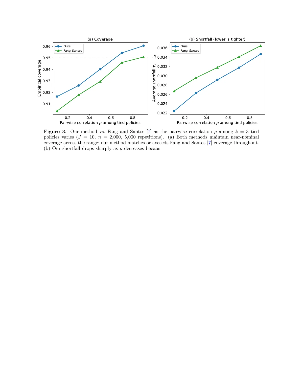
Empirical Lik eliho o d for Nonsmo oth F unctionals Hongseok Namk o ong Decision, Risk, and Op erations Division, Colum bia Business Sc ho ol namkoong@gsb.columbia.edu Abstract Empirical lik eliho od is an attractive inferential framework that resp ects natural parameter b oundaries, but existing approac hes t ypically require smoothness of the functional and mis- calibrate substan tially when these assumptions are violated. F or the optimal-v alue functional cen tral to p olicy ev aluation, smo othness holds only when the optimum is unique—a condition that fails exactly when rigorous inference is most needed where more complex p olicies hav e mo dest gains. In this w ork, we dev elop a b o otstrap empirical likelihoo d method for partially nonsmo oth functionals. Our analytic w orkhorse is a geometric reduction of the proﬁle lik eli- ho o d to the distance b et w een the score mean and a level set whose shap e (a tangent cone given b y nonsmoothness patterns) determines the asymptotic distribution. Unlike the classical pro of tec hnology based on T a ylor expansions on the dual optima, our geometric approach leverages prop erties of a deterministic conv ex program and can directly apply to nonsmo oth functionals. Since the ordinary bo otstrap is not v alid in the presence of nonsmo othness, w e deriv e a corrected m ultiplier b o otstrap approach that adapts to the unkno wn level-set geometry . 1 In tro duction Empirical likelihoo d (EL) is a nonparametric method of inference that retains many of the virtues of parametric likelihoo d without committing to a parametric mo del. Giv en data X 1 , . . . , X n , one maximizes the pro duct Q n i =1 p i o ver probabilit y vectors ( p 1 , . . . , p n ) sub ject to the constrain t that a parameter of in terest tak es a h yp othesized v alue. The resulting lik eliho o d-ratio statistic conv erges to χ 2 under the null, yielding conﬁdence regions that are automatically shap ed b y the data, re- sp ect natural parameter boundaries, and satisfy a Bartlett correction [ 18 ]. Because the construction requires no v ariance estimation and no distributional sp eciﬁcation, EL conﬁdence regions ha ve com- plemen tary adv antages to normal-theory counterparts in ﬁnite samples: they are range-resp ecting, transformation-in v ariant, and self-normalizing. These prop erties hav e made EL an attractive foun- dation for inference on means, quantiles, regression parameters, and smo oth functions thereof. F or a decision-maker choosing among comp eting options under uncertain ty , the app eal of EL is esp ecially direct. The shap e adaptation means that conﬁdence regions con tract along directions the data resolve w ell and expand where they do not, so the resulting b ounds on decision-relev an t quan tities are neither artiﬁcially wide nor miscalibrated. This pap er is motiv ated by whether these adv antages can be extended to a class of problems that is cen tral to mo dern data-driven decision- making but falls outside the scop e of existing EL theory: inference on the av erage reward under the b est av ailable p olicy , which often guides in v estment decisions for interv en tions with an initial ﬁxed setup cost. Motiv ating application A large and growing class of decision problems requires ev aluating candidate policies from data collected under a diﬀerent, unkno wn b ehavioral p olicy . In healthcare, a clinician considering a new treatment assignmen t rule sees only the outcomes of the assignments 1 that w ere actually made; in e-commerce, a platform testing pricing strategies observes rev enue only under the prices that were historically charged. F ormally , the observed data consist of cov ariates, an action or treatment drawn from the b eha vioral p olicy , and an outcome. The decision-maker has sev eral candidate p olicies, each mapping cov ariates to actions, and the quan tity of in terest is the v alue of the best a v ailable option, τ ( P 0 ) = max 1 ≤ j ≤ J { θ j ( P 0 ) := E P 0 [ Y π j ] } , (1) where Y π j is the potential outcome under p olicy π j . Because the counterfactual outcomes are not directly observed, estimating eac h p olicy v alue requires modeling n uisance functions—the prop ensit y score and the conditional outcome means— making the problem gen uinely semiparametric. Ov er the past decade, the double/debiased mac hine learning (DML) literature has provided a clean reduction of this diﬃculty [ 4 ]. After splitting the sample and ﬁtting n uisance mo dels on an auxiliary fold, one forms augmen ted inv erse-probabilit y w eighting (AIPW) scores on the ev aluation fold: X ni,j = b m π j ( W i ) ( W i ) + ⊮ { A i = π j ( W i ) } b e π j ( W i ) ( W i )  Y i − b m A i ( W i )  , j = 1 , . . . , J. (2) Under standard o v erlap and rate conditions on the n uisance estimators [ 4 , 1 , 12 ], the score v ec- tor satisﬁes a cen tral limit theorem centered at the true p olicy-v alue v ector, and its sample mean con verges at √ n -rate. The debiasing step thus conv erts a semiparametric problem into a nonpara- metric one: inference on the maximum of a √ n -normal score mean. Given these score vectors, it is natural to apply empirical likelihoo d. Wh y are ties relev an t? In man y applied settings, the primary question is not “which p ol- icy is b est?” but “do es the b est av ailable p olicy improv e enough ov er a simple default to justify its implementation cost?” A decision-maker comparing a complex p ersonalized treatmen t rule (whic h requires exp ensiv e real-time data collection and infrastructure) against a simpler rule that ignores certain co v ariates is p erforming exactly this kind of opp ortunity sizing. A growing b o dy of empirical w ork suggests that the gains from personalization are often modest: in education, p erson- alized tutoring p olicies frequen tly oﬀer only marginal impro vemen ts o ver static alternativ es [ 16 ]; in healthcare, heterogeneous treatment eﬀects are routinely small relative to a v erage eﬀects [ 5 ]; and in welfare-maximizing p olicy design, the impro v emen t from targeting ov er a uniform rule can b e negligible [ 13 ]. When sev eral candidate policies ac hieve similar expected rew ards, the set of optimal p olicies con tains multiple elements—and it is in this near-tied regime that a rigorous conﬁdence b ound on the b est attainable v alue is most decision-relev ant. It is also where existing metho ds break down. Limitations of existing EL approaches The existing EL mac hinery , how ever, do es not accom- mo date the nonsmo oth max functional ( 1 ). Both classical EL results for nonlinear functionals [ 18 , 6 ] and semiparametric EL extensions [ 8 , 3 ] require that the target map b e smo oth. Molanes-L´ op ez et al. [ 15 ] study EL for non-smo oth criterion functions, but their framew ork targets U-statistics and related criteria rather than the directionally diﬀeren tiable max functional that arises in p olicy ev al- uation. Applying them to ( 1 ) forces one of tw o w ork arounds. The ﬁrst is pr oje cte d joint EL : build a join t conﬁdence region for the full p olicy-v alue v ector and pro ject on to the maximum. This is v alid but pa ys a dimension- J critical v alue for a scalar target; at the 95% level with t wen ty p olicies, the 2 resulting b ound is signiﬁcan tly wider than necessary (Proposition 5 ). The second is sele cte d-p olicy EL : estimate the empirically b est p olicy and run one-dimensional EL on that co ordinate. This ignores selection uncertain ty and underco v ers badly near ties. Bey ond the conserv atism-v ersus-co verage tradeoﬀ, semiparametric bo otstrap calibration can create a computational b ottleneck. The b o otstrap metho d of Hjort et al. [ 8 ] requires reﬁtting all n uisance mo dels inside every resample, turning a mo derate inferential problem in to an exp ensive learning problem rep eated hundreds of times. F or smo oth targets, Brav o et al. [ 3 ] sidestep this cost by replacing the original momen t with an inﬂuence-function-corrected equation, restoring the Wilks prop ert y without resampling-lev el reﬁtting. Their ﬁx, ho wev er, relies on smo othness of the target functional and do es not extend to the nonsmo oth max functional ( 1 ). A further diﬃcult y is nonregularit y . When one p olicy is uniquely optimal, the max functional is Hadamard diﬀerentiabl e (HD) and a standard χ 2 calibration applies [ 6 ]. But the uniqueness assumption is itself at least as hard to verify as the inferential task: certifying that one p olicy is strictly b etter than all others requires the same kind of statistical evidence as the conﬁdence b ound one is trying to construct. When tw o or more policies are tied or near-tied—the regime argued ab ov e to b e the most decision-relev ant—the max functional is only Hadamard directionally diﬀeren tiable (HDD) and the geometry of the problem c hanges. The lo cal lev el set is no longer a hyperplane but a c one whose faces corresp ond to diﬀeren t tie-breaking patterns among the optimal p olicies. The standard χ 2 1 calibration, which is correct for h yp erplanes, systematically underestimates the critical v alue for cones b ecause it ignores this combinatorial face structure. The ordinary bo otstrap inherits this failure: it alw ays estimates the lev el set as a hyperplane (since sample ties o ccur with probabilit y zero), and therefore conv erges to χ 2 1 regardless of the true geometry [ 7 ]. Our exp erimen ts in Section 6 sho w that cov erage drops well b elo w the nominal level when t w o or more p olicies are near-tied. Corrected b o otstrap metho ds for nonsmo oth functionals exist [ 7 , 9 , 10 , 2 ], but they target plug-in estimators rather than proﬁle-divergence statistics and do not inherit the shap e-resp ecting, self-normalizing prop erties that mak e EL attractive in the ﬁrst place. 1.1 Con tributions W e dev elop a sc or e-pr oﬁle empiric al likeliho o d that targets the optimal v alue directly . When applied to our motiv ating problem, our metho d op erates on the AIPW score vectors ( 2 ) pro duced by a single nuisance ﬁt and requires no reﬁtting inside the b o otstrap loop. Our central tec hnical contribution is a primal geometric pro of strategy that replaces the dual Lagrange-m ultiplier expansion used in classical EL theory . In the standard approach—dev elop ed b y Ow en [ 18 ] and extended to semiparametric settings by Hjort et al. [ 8 ] and Brav o et al. [ 3 ]— one writes the EL ratio as a function of a dual parameter (the Lagrange m ultiplier enforcing the momen t constraint), p erforms a T aylor expansion of the dual optimalit y conditions around the true parameter v alue, and inv erts to obtain an asymptotic χ 2 limit. This dual route works well for smo oth estimating equations, but it encounters t wo obstacles for nonsmo oth targets like ( 1 ): the proﬁle ov er the nonsmo oth lev el set do es not reduce to a single moment constraint with a smo oth Lagrangian, so the standard KKT expansion has no smo oth analogue. Our primal pro of a v oids this obstacle b y w orking directly in the weight sp ac e of the empirical lik eliho o d. The k ey reduction (Theorem 1 ) shows that the Euclidean proﬁle statistic—the minim um ℓ 2 distance from uniform w eights to the set of rew eightings consisten t with the target v alue—equals the Mahalanobis distance from the score mean to the rescaled level set. This is a ﬁnite-dimensional con vex pro jection whose b eha vior dep ends entirely on the geometry of the target map, not on 3 the mechanics of a dual expansion. Whether the level set is lo cally a hyperplane or a cone then determines the asymptotic distribution and b o otstrap v alidity . In the smo oth (HD) case, the lev el set conv erges to a hyperplane, the Mahalanobis pro jection is a scalar ratio, and the proﬁle statistic con verges to χ 2 1 . An ordinary score bo otstrap—applied to the frozen score v ectors, with no n uisance reﬁt—is consistent (Theorem 6 ). In the nonsmo oth (HDD) case, the level set conv erges to a tangen t cone, the limit b ecomes the squared Mahalanobis distance from a Gaussian v ector to this cone, and the ordinary b o otstrap fails. W e dev elop a corrected calibration pro cedure based on a m ultiplier b o otstrap approac h (Theorem 9 ) that estimates the tangent cone from the data and computes the b o otstrap distance to the estimated cone. The same conclusions extend to general smo oth f -div ergences under a lo cal quadratic-geometry condition, b ecause the primal argumen t nev er in vok es a F enchel conjugate and therefore imposes no smoothness conditions on the div ergence beyond lo cal quadratic b eha vior near the uniform distribution. W e note t wo diﬀerences from existing semiparametric EL frameworks. First, the en tire primal analysis is deterministic once the score array is given: the geometric reduction is a statemen t ab out the structure of a con vex program, not about the probabilistic b eha vior of a dual optimizer. This makes the extension to the b o otstrap immediate—the same conv ex pro jection is applied to the b o otstrap score v ectors, and cone estimation handles the nonsmo oth case. By contrast, the standard dual approac h (e.g., Hjort et al. [ 8 ]) requires a sto chastic expansion of the Lagrange m ultiplier that m ust b e controlled uniformly o ver b o otstrap resamples, an analysis whose diﬃculty scales with the complexity of the momen t condition and that has no natural extension to nonsmo oth targets. Second, b ecause the geometric reduction op erates on the score array rather than on the original data, the b o otstrap inherits the score-lev el structure: once the AIPW scores ha v e b een formed, ev ery subsequent computation is O ( nJ ) p er resample, with no reference to the nuisance mo dels. An y semiparametric EL metho d whose bo otstrap is coupled to the nuisance-estimation step— including the framew ork of Hjort et al. [ 8 ]—must reﬁt all nuisance models inside ev ery resample, turning eac h b o otstrap dra w in to a full semiparametric learning problem. Even in our small-scale sim ulations, this diﬀerence leads to multiple orders of magnitude improv ement in computational eﬀort. Although w e dev elop the theory in detail for the max functional—the leading case in p ol- icy ev aluation and one whose combinatorial structure yields closed-form proﬁle b ounds—the core results (the primal geometric reduction, the level-set characterization, and b oth b o otstrap pro ce- dures) apply to any functional satisfying Assumption B , including other Hadamard directionally diﬀeren tiable maps such as quan tile and suprem um-norm functionals. 2 Related w ork Our work connects four strands of literature. Classical empirical lik eliho o d. Since Owen [ 17 ]’s seminal work that developed the theory of empirical lik eliho o d for means, several authors ha ve extended the framework to smooth functions of means and regression settings, and established the χ 2 calibration, Bartlett correctabilit y , and range-resp ecting property (see [ 18 ] and references therein). Our primal pro of strategy can be view ed as revisiting Owen’s original lik eliho o d-ratio construction from the weigh t-space p ersp ective 4 rather than the classical dual Lagrange multiplier persp ective [ 18 ], and showing that this viewpoint extends naturally to directionally diﬀerentiable maps where the dual route encoun ters fundamental obstructions. In particular, compared to Duc hi et al. [ 6 ]’s recen t generalized EL result for Hadamard diﬀeren tiable functionals, our approac h provides calibrated conﬁdence in terv als even for Hadamard diﬀeren tiable functionals suc h as the inﬁmum functional when there is multiple optima. Molanes- L´ op ez et al. [ 15 ] extend EL to non-smo oth criterion functions such as absolute deviations and U- statistics, establishing a Wilks-t yp e theorem under a lo cal smo othing device. Their non-smo othness is of a diﬀerent kind from ours: it lies in the criterion used to deﬁne the EL constraint, whereas in our setting the moment conditions are smo oth but the functional mapping scores to the target parameter is only directionally diﬀeren tiable. Semiparametric empirical lik eliho o d. Hjort et al. [ 8 ] extend empirical lik eliho o d to plug- in n uisance parameters and slow er-than- √ n rates, establishing both a Wilks phenomenon and b o otstrap v alidit y for semiparametric estimating equations. Their results are broad and p ow erful but require that the target b e deﬁned as the solution to a smo oth momen t condition; the max functional ( 1 ) do es not hav e this structure. Brav o et al. [ 3 ] sho w that naive tw o-step plug-in EL can fail to hav e a χ 2 limit even for smo oth targets—the n uisance estimation bias con taminates the EL ratio—and restore the Wilks prop erty by replacing the original moment with an inﬂuence- function-corrected equation. Their correction is essen tial for any practical semiparametric EL implemen tation, but lik e Hjort et al. [ 8 ] it applies to smo oth estimating equations. Our con tribution departs from b oth b y proﬁling the tar get functional itself —rather than an estimating equation whose solution equals the target—and b y handling the nonsmooth case where the level-set geom etry is a cone rather than a h yp erplane. Debiased inference and p olicy ev aluation. Chernozh uko v et al. [ 4 ] develop the double/debiased mac hine learning framew ork, providing general conditions under whic h cross-ﬁtted orthogonal scores achiev e √ n -normalit y for semiparametric targets even when n uisance functions are esti- mated at slow er-than-parametric rates. This framew ork supplies the score vectors that our metho d tak es as input. Athey and W ager [ 1 ] adapt these ideas to p olicy learning and oﬀ-p olicy ev aluation, deriving regret b ounds and inference for individual p olicy v alues under treatment-eﬀect hetero- geneit y . In a complementary direction, Li and Brunskill [ 14 ] study optimal v alue inference in the semiparametric setting and deriv e debiased semiparametric eﬃciency guaran tees under uniqueness of optima. Our contribution is in what happ ens after the scores are formed: constructing a proﬁle- div ergence statistic for the nonlinear scalar target and calibrating it correctly in both the smo oth and nonsmo oth regimes. Inference for nonsmo oth functionals. When tw o or more p olicies are tied for optimality , the max functional ( 1 ) is only (Hadamard) directionally diﬀeren tiable, and the ordinary bo otstrap fails. F ang and San tos [ 7 ] dev elop a general b o otstrap correction for directionally diﬀerentiable maps, es- tablishing consistency of a plug-in m ultiplier b o otstrap under cone-appro ximation conditions. Their framew ork is the closest an tecedent to our nonsmooth theory; the diﬀerence is that they calibrate a plug-in estimator while w e calibrate a proﬁle-divergence statistic. The t wo approac hes draw on the same lo cal cone information but pro duce diﬀerent inferen tial ob jects: a corrected conﬁdence in terv al versus a directly in vertible proﬁle b ound. Hong and Li [ 9 ] provide b o otstrap consistency results for directionally diﬀerentiable functions with applications to conditional v alue-at-risk and 5 related risk measures; Hong and Li [ 10 ] extend the analysis to M-estimators of nonsmo oth pa- rameters. Our w ork studies the same directional diﬀerentiabilit y structure but in the empirical lik eliho o d framework, whic h yields the simplex formulation of Prop osition 4 and the computational adv antages of score-lev el resampling. The remainder of the pap er is organized as follo ws. Section 3 in tro duces the score-proﬁle framew ork and establishes the cen tral geometric reduction that connects the proﬁle statistic to a Mahalanobis distance to a level set. Section 4 develops the smo oth (Hadamard diﬀerentiable) case, derives closed-form proﬁle bounds for the p olicy problem, and sho ws that an ordinary score b o otstrap is consistent. Section 5 handles the nonsmo oth case of tied p olicies, dev elops the corrected m ultiplier bo otstrap, and describes the full inferen tial procedure. Section 6 rep orts simul ation evidence on co verage, tightness, and computation time. 3 Score-proﬁle framew ork and geometric reduction W e b egin b y developing our inferential framework. First, w e deﬁne the score-proﬁle div ergence statistic that underpins all subsequen t results, then state the score regularity conditions and the running p olicy-ev aluation example (Section 3.1 ). Section 3.2 establishes the cen tral geometric reduction that connects the proﬁle statistic to a Mahalanobis distance, and Section 3.3 sho ws ho w the ﬁrst-order shape of the target functional’s lev el set determines the limiting distribution. Our inferential primitiv e is a triangular array of score v ectors X n 1 , . . . , X nn ∈ R d obtained after sample splitting and n uisance estimation. In policy ev aluation, the auxiliary sample is used to ﬁt prop ensit y and outcome models, and the ev aluation sample pro duces doubly robust scores for eac h candidate policy (see Example 1 in Section 3.1 for details). Giv en the score arra y , let ϕ : R d → R b e the target map with τ 0 = ϕ ( θ 0 ), and let f : R + → R ∪ { + ∞} be con v ex with f (1) = f ′ (1) = 0 and f ′′ (1) = 2. The sc or e-pr oﬁle f -diver genc e statistic is R n,f ( τ 0 ) := inf q ∈ ∆ n n nD f ( q ∥ 1 /n ) : ϕ  P n i =1 q i X ni  = τ 0 o , (3) where ∆ n = { q ≥ 0 : P i q i = 1 } and D f ( q ∥ 1 /n ) = n − 1 P n i =1 f ( nq i ). The Euclidean case f 2 ( t ) = ( t − 1) 2 will play a distinguished role: R n, 2 ( τ 0 ) := inf q ∈ ∆ n n P n i =1 ( nq i − 1) 2 : ϕ  P n i =1 q i X ni  = τ 0 o . (4) The statistic ( 3 ) proﬁles out the scalar target τ 0 while reweigh ting the score vectors, so that the in- feren tial problem reduces to a ﬁnite-dimensional divergence minimization on the already-computed scores. No nuisance model is revisited after the scores ha ve b een formed. W e fo cus on the χ 2 div er- gence to deﬁne proﬁles for the rest of this work and omit the extensions to the general f -div ergence case as it is a consequence of tedious T aylor expansions. 3.1 Score regularit y W e w ork directly with the score array and impose the follo wing high-level regularity condition. Assumption A (Score regularity) . Ther e exists a p ositive deﬁnite matrix Σ such that, writing ¯ X n = 1 n n X i =1 X ni , b Σ n = 1 n n X i =1 ( X ni − ¯ X n )( X ni − ¯ X n ) ⊤ , Z n = √ n ( ¯ X n − θ 0 ) , 6 the fol lowing hold: (i) Z n ⇒ Z ∼ N (0 , Σ) ; (ii) b Σ n p → Σ ; (iii) max 1 ≤ i ≤ n ∥ X ni − ¯ X n ∥ / √ n p → 0 . Condition (iii) is a Lindeb erg-type negligibility requirement that follo ws, for instance, from a uniform (2 + δ )-moment b ound. The assumption is standard in the double/debiased machine learning literature and holds for augmented in v erse-probabilit y w eighting scores under mild o v erlap and rate conditions on the nuisance estimators [ 4 , 1 , 12 ]. Example 1 (Policy ev aluation with doubly robust scores) : Let W denote cov ariates, a binary treatmen t assignmen t A ∈ { 0 , 1 } , and an observ ed outcome Y ∈ R . W rite Y ( a ) for the p otential outcome under treatment a , and let Π = { π 1 , . . . , π J } b e a ﬁnite class of deterministic p olicies π j : W → { 0 , 1 } . The p olicy v alue is V π ( P 0 ) = E [ Y ( π ( W )) ], and the target of inference is the b est p olicy v alue τ ( P 0 ) = max 1 ≤ j ≤ J V π j ( P 0 ). Deﬁne the prop ensity score e 0 ( w ) = P ( A = 1 | W = w ) and the conditional outcome functions m 0 ,a ( w ) = E [ Y | W = w, A = a ] for a ∈ { 0 , 1 } . W e imp ose the following standard conditions on the data-generating process and the n uisance estimators. (a) Unc onfounde dness. ( Y (0) , Y (1) ) ⊥ A | W . (b) Overlap. There exists η > 0 suc h that η ≤ e 0 ( w ) ≤ 1 − η for P 0 -almost every w . (c) Moment c ondition. There exists δ > 0 suc h that E [ | Y | 2+ δ ] < ∞ . (d) Sample splitting. The data are split into an auxiliary sample (used to ﬁt n uisance estimators b e, b m 0 , b m 1 ) and an indep enden t ev aluation sample of size n . The ev aluation-sample observ ations ( W i , A i , Y i ) n i =1 are i.i.d. conditional on the auxiliary s ample. (e) R ate c ondition. The n uisance estimators satisfy the pro duct rate ∥ b e − e 0 ∥ L 2 ( P 0 ) · max a ∈{ 0 , 1 } ∥ b m a − m 0 ,a ∥ L 2 ( P 0 ) = o p ( n − 1 / 2 ) , and each factor is o p (1). Conditions (a) and (b) are the standard iden tifying assumptions for causal inference from observ a- tional data [ 19 , 11 ]. Condition (e) is the doubly robust rate requirement: it permits eac h nuisance function to con verge slo wer than the n − 1 / 4 rate, so long as the pro duct of the tw o rates is o ( n − 1 / 2 ). This accommo dates mo dern nonparametric and machine-learning estimators; see Chernozh uko v et al. [ 4 ] for suﬃcien t conditions using cross-ﬁtting, and A they and W ager [ 1 ] and Kallus and Uehara [ 12 ] for adaptations to the policy ev aluation setting. Giv en these conditions, the ev aluation-sample AIPW scores X ni,j = b m π j ( W i ) ( W i ) + ⊮ { A i = π j ( W i ) } b e π j ( W i ) ( W i )  Y i − b m A i ( W i )  , j = 1 , . . . , J, satisfy Assumption A . The CL T (condition (i) ) and co v ariance consistency (condition (ii) ) follow from the double robustness of the AIPW estimator: the pro duct rate condition (e) ensures that 7 the bias from nuisance estimation is o p ( n − 1 / 2 ), so the scores b ehav e asymptotically as if the true n uisance functions w ere kno wn. The Lindeberg condition (iii) follo ws because the o verlap b ound (b) and the (2 + δ )-moment assumption (c) imply E [ | X ni,j | 2+ δ ] < ∞ uniformly in j , whic h is a standard suﬃcien t condition for Lindeberg negligibilit y in the triangular-arra y setting. ⋄ 3.2 Geometric reduction Starting with Ow en [ 17 ]’s seminal work, the standard route to EL asymptotics is b y using the dual reformulation: one writes the score-proﬁle statistic as a function of a Lagrange multiplier enforcing the moment constraint, p erforms a sto chastic T aylor expansion of the KKT conditions around the true parameter, and inv erts to obtain a χ 2 limit [ 18 , 8 ]. This dual route encounters t wo obstacles for nonsmo oth targets like τ = max j θ j . First, the proﬁle ov er the nonsmo oth level set do es not reduce to a single moment constrain t with a smo oth Lagrangian, so the standard KKT expansion has no smooth analogue. Second, even in the smooth case, a dual b o otstrap pro of requires a uniform smallness condition on the resampled Lagrange m ultiplier—a conditional empirical-pro cess argumen t in tert wined with the KKT expansion—that becomes esp ecially delicate when n uisance functions are reﬁt inside each resample. A formal dual representation and a detailed comparison are giv en in App endix A (Prop osition 11 ). Instead, we tak e a direct primal approach in this pap er. W e work directly in the w eigh t space of the empirical lik eliho o d and show that the proﬁle statistic admits an exact geometric in terpretation. Sp eciﬁcally , it equals the squared Mahalanobis distance from the score mean to the lev el set of the target map. F or t > 0, deﬁne the lo c al level set L t := { v ∈ R d : ϕ ( θ 0 + tv ) = τ 0 } . This is the set of all rescaled p erturbation directions along whic h the target functional retains its null-h yp othesized v alue. See App endix A.1 for the proof of the follo wing result. Theorem 1 (Geometric reduction) . Under Assumption A , R n, 2 ( τ 0 ) = d 2 b Σ n ( Z n , L 1 / √ n ) + o p (1) , wher e d 2 A ( z , S ) := inf v ∈ S ( z − v ) ⊤ A − 1 ( z − v ) for p ositive deﬁnite A and close d S ⊂ R d . T o see wh y this is true, consider what the proﬁle statistic ( 4 ) is actually computing. The problem is to ﬁnd probability w eigh ts ( q 1 , . . . , q n ) that make the weigh ted mean P i q i X ni satisfy the target constraint ϕ ( · ) = τ 0 , while staying as close as p oss ible to the uniform weigh ts q i = 1 /n in the squared-deviation sense P i ( nq i − 1) 2 . Reparameterizing the constraint b y writing the weigh ted mean as θ 0 + n − 1 / 2 v for some direction v ∈ L 1 / √ n , the problem b ecomes: for each direction v on the level set, what is the cheapest wa y to tilt the empirical weigh ts so that the reweigh ted mean lands at θ 0 + n − 1 / 2 v ? This tilting problem is a minim um-norm least-squares problem. With a i = nq i − 1 as the p erturbation from uniform and U ni = X ni − ¯ X n as the centered scores, the constraint b ecomes P i a i U ni = √ n ( v − Z n ) with cost P i a 2 i . The minim um-norm solution is a ni ( v ) = 1 √ n U ⊤ ni b Σ − 1 n ( v − Z n ) , (5) with total cost ( v − Z n ) ⊤ b Σ − 1 n ( v − Z n )—the squared Mahalanobis distance from the score mean Z n to the p oin t v . The key observ ation is that the p ositivity constraints 1 + a i ≥ 0 are asymptotically 8 inactiv e: the optimal p erturbations a ni ( v ) are of order n − 1 / 2 uniformly o v er bounded v , so the w eights q i = (1 + a i ) /n are strictly p ositiv e for all large n (the formal statement and proof are given in App endix A.1.1 , Prop osition 10 ). Minimizing the Mahalanobis cost o v er all directions v on the level set gives Theorem 1 . The en tire argumen t is deterministic once the score arra y is giv en: it is a statement ab out the structure of a con vex program, not about the sto c hastic b eha vior of a dual optimizer. No T aylor expansion of an optimized Lagrangian is needed, and no Gaussianit y of the scores is inv oked. The randomness en ters only through Z n and b Σ n , and the geometric question that remains is purely ab out the shap e of the lev el set L 1 / √ n . 3.3 Lev el sets to limiting distributions By Theorem 1 , the proﬁle statistic reduces to the squared Mahalanobis distance from Z n to the lev el set L 1 / √ n . Since Z n ⇒ Z ∼ N (0 , Σ), the limiting distribution of R n, 2 ( τ 0 ) is determined b y the ﬁrst-order shap e to which L 1 / √ n con verges as n grows. T o make this concrete, return to the motiv ating example. The max functional τ = max j θ j applied to J p olicy v alues has level set L t = { v ∈ R J : max 1 ≤ j ≤ J ( θ 0 j + tv j ) = τ 0 } . This is the set of all local p erturbation directions v that preserve the b est p olicy v alue at τ 0 . F or small t , the suboptimal p olicies—those with θ 0 k strictly b elo w τ 0 —are irrelev ant: their p erturb ed v alues θ 0 k + tv k remain b elow τ 0 as long as v sta ys bounded. The constraint therefore inv olves only the optimal p olicies J 0 = arg max j θ 0 j . Tw o cases arise. If a single policy is uniquely optimal ( | J 0 | = 1, sa y J 0 = { j 0 } ), then the constrain t reduces to v j 0 = 0: a hyp erplane in R J . As we will show in subsequen t sections, pro jecting Z n on to a hyperplane pro duces a scalar ratio that con verges to χ 2 1 —the familiar Wilks phenomenon. If tw o or more p olicies are tied for optimality ( | J 0 | > 1), the constrain t b ecomes max j ∈ J 0 v j = 0: a c one whose faces corresp ond to the diﬀerent tie-breaking patterns. Pro jecting Z n on to a cone yields a non- χ 2 limit that depends on the geometry of the cone and the co v ariance Σ. In b oth cases, L t con verges to a well-deﬁned limit set C as t ↓ 0, and the nature of C — h yp erplane or cone—determines the asymptotic distribution. The practitioner do es not need to kno w which case applies: whether | J 0 | = 1 or | J 0 | > 1 is itself an inferen tial question that is at least as hard as the conﬁdence b ound b eing sought, so any method that requires assuming uniqueness a priori is circular. Our framework handles b oth geometries with a single pro cedure by estimating C from the data (Section 5 ). The following assumption formalizes this conv ergence for a general target functional. Assumption B (Level-set conv ergence) . Ther e exists a close d set C ⊂ R d such that for every ﬁxe d M < ∞ , d H ( L t ∩ B M , C ∩ B M ) → 0 as t ↓ 0 , wher e d H denotes Hausdorﬀ distanc e and B M = { v : ∥ v ∥ ≤ M } . Assumption B is the only structural condition the subsequent theory requires of the target functional ϕ . In particular, the geometric reduction (Theorem 1 ), the asymptotic distribution (Theorem 3 ), and both b o otstrap pro cedures (Theorems 6 and 9 ) hold for an y ϕ satisfying this as- sumption; we dev elop the max functional in detail because it is the leading case in policy ev aluation and its com binatorial structure yields closed-form proﬁle b ounds. 9 The role of the truncation at radius M is technical: it ensures that conv ergence is stated on compacts, which suﬃces b ecause the minimizing pro jection in Theorem 1 lies in a b ounded region with high probabilit y . F or the max functional, the informal argumen t abov e can b e made precise. Prop osition 2 (Level-set structure of the max functional) . L et ϕ ( θ ) = max 1 ≤ j ≤ J θ j . If ∆ 0 := min k / ∈ J 0 ( τ 0 − θ 0 k ) > 0 (with ∆ 0 = + ∞ when J 0 = { 1 , . . . , J } ), then for every ﬁxe d M < ∞ and every 0 < t < ∆ 0 / M , L t ∩ B M = { v ∈ B M : max j ∈ J 0 v j = 0 } . Conse quently: (i) If | J 0 | = 1 , Assumption B holds with C = H = { v : v j 0 = 0 } , a hyp erplane. (ii) If | J 0 | > 1 , Assumption B holds with C = { v : max j ∈ J 0 v j = 0 } , a c one. Pr o of. See Appendix B.1 . Assumption B paired with Theorem 1 now reduces the calibration problem to understanding d 2 Σ ( Z, C ) for the appropriate limit set C . See App endix A.2 for a formal deriv ation. Theorem 3 (Distance-to-set limit) . Under Assumptions A and B , R n, 2 ( τ 0 ) = d 2 b Σ n ( Z n , C ) + o p (1) ⇒ d 2 Σ ( Z, C ) , Z ∼ N (0 , Σ) . Theorem 3 reduces the problem of calibrating the proﬁle statistic to identifying the ﬁrst-order limit set C . When C is a h yp erplane, the distance d 2 Σ ( Z, C ) is a scalar quadratic form and the limit is χ 2 1 —the standard Wilks calibration (Section 4 ). When C is a cone, ho wev er, the calibration problem is harder. The distance d 2 Σ ( Z, C ) is the minim um of a quadratic form ov er the faces of C , eac h face corresp onding to a diﬀerent subset of the tied p olicies that could attain the maximum. The resulting limit is a w eigh ted mixture of χ 2 distributions ( ¯ χ 2 ) whose mixing probabilities dep end on the unkno wn cone C and the co v ariance Σ—a non-piv otal distribution that cannot be tabulated. Applying the standard χ 2 1 critical v alue in this setting amoun ts to pro jecting onto a single face (the tangen t h yp erplane), ignoring all other faces of the cone, and systematically underestimates the true critical v alue. Section 5 develops a corrected b o otstrap that estimates the c one from the data and pro duces the correct critical v alue without requiring the practitioner to kno w J 0 . 4 Smo oth Statistical F unctionals Before turning to the main results of this pap er—b o otstrap calibration for nonsmooth functionals— w e develop the theory for smo oth targets. The smo oth case serves an exp ository and illustrative purp ose: it sho ws that the geometric framework recov ers classical results (the Wilks χ 2 1 limit and ordinary b o otstrap consistency) as sp ecial cases, and it introduces the closed-form proﬁle b ounds and the standard bo otstrap approac h. Existing EL results for the max functional [ 6 ] assume | J 0 | = 1 throughout, which, as we argued in Section 1 , is at least as hard to verify as the inferential task itself. Our framework will ultimately remo ve this requirement (Section 5 ), but the smo oth case is the natural starting p oint b ecause it isolates the geometric mechanism. When the target functional ϕ is Hadamard diﬀerentiable at θ 0 with nonzero gradien t a 0 = ∇ ϕ ( θ 0 ), the lo cal level set conv erges to a hyperplane H = { v : a ⊤ 0 v = 0 } . This is the smo oth case: the proﬁle statistic conv erges to χ 2 1 , reco vering the classical Wilks phenomenon, and an 10 ordinary score b o otstrap is consisten t. W e now develop these results and instantiate them for the p olicy ev aluation problem. Recall that J 0 = arg max j θ 0 j denotes the set of optimal p olicies. By Prop osition 2 (i), when a single p olicy is uniquely optimal ( | J 0 | = 1, say J 0 = { j 0 } ) the level set is the hyperplane H = { v : v j 0 = 0 } . W e formalize this as an assumption on the general target functional. Assumption C (Hyp erplane regularit y) . Assumption B holds with C = H for a hyp erplane H = { v : a ⊤ 0 v = 0 } with a 0  = 0 . Corollary 1 (Smo oth limit) . Under Assumptions A and C , R n, 2 ( τ 0 ) = ( a ⊤ 0 Z n ) 2 a ⊤ 0 b Σ n a 0 + o p (1) ⇒ χ 2 1 . Pr o of. See Appendix A.3 . The squared Mahalanobis distance from a Gaussian v ector to a h yp erplane is a scalar ratio χ 2 1 — this is simply the statemen t that the signed distance from Z n to H , normalized by the appropriate v ariance, is asymptotically standard normal. F or the max functional with a unique optimum at p olicy j 0 , the proﬁle statistic reduces to n ( ¯ X n,j 0 − τ 0 ) 2 / b Σ n,j 0 j 0 + o p (1): the squared t -statistic for the best policy’s v alue. The EL mac hinery pro duces the familiar W ald-t yp e test as a sp ecial case, but with the imp ortant diﬀerence that the critical v alue has b een derived from the proﬁle geometry rather than from a v ariance estimation. 4.1 Closed-form proﬁle b ounds Because the max functional has combinatorial structure, the proﬁle statistic can b e expressed in closed form. The closed-form expressions sho w how the proﬁle statistic dep ends on the p olicy- v alue gaps and cov ariance structure, and they serve as the foundation for the simplex low er-b ound form ula used in both the smo oth and nonsmo oth cases. The max functional’s combinatorial structure allows the geometric ob jects in Theorem 1 to b e computed in closed form. By Theorem 1 , the Euclidean proﬁle statistic for the max target is R max n, 2 ( τ ) = n d 2 b Σ n ( ¯ X n , M τ ) + o p (1) , (6) where M τ = { m ∈ R J : max j m j = τ } . F or the decision-maker’s primary ob ject of interest—a lo wer conﬁdence b ound on the b est p olicy v alue—the proﬁle statistic admits a particularly clean dual form. Prop osition 4 (Lo wer b ound via simplex optimization) . F or a critic al value c > 0 , deﬁne the ac c eptanc e el lipsoid E n ( c ) = { m ∈ R J : n ( m − ¯ X n ) ⊤ b Σ − 1 n ( m − ¯ X n ) ≤ c } . The lower endp oint L n ( c ) := inf m ∈ E n ( c ) max j m j satisﬁes L n ( c ) = max w ∈ ∆ J  w ⊤ ¯ X n − r c n q w ⊤ b Σ n w  , ∆ J = { w ≥ 0 , w ⊤ ⊮ = 1 } . This result is known [ 6 ], and we rederiv e it for completeness in Appendix B.3 . The simplex repre- sen tation is computationally attractive: after the score mean and co v ariance hav e been computed, the low er b ound is obtained b y solving a J -dimensional con vex program rather than manipulating 11 n empirical-lik eliho o d w eights. The optimal weigh t v ector w ∗ is concen trated on the near-optimal p olicies, so in practice the program eﬀectiv ely reduces to a problem of dimension | J 0 | . The leading-order cost of the pro jected-join t work around discussed in Section 1 can also b e made precise. Recall that ∆ 0 = min k / ∈ J 0 ( τ 0 − θ 0 k ) is the gap b etw een the best p olicy v alue and the second-b est. Prop osition 5 (Inﬂation factor) . Supp ose | J 0 | = 1 with ∆ 0 > 0 . L et c 1 ,α = χ 2 1 , 1 − α and c J,α = χ 2 J, 1 − α . Then the dir e ct pr oﬁle lower b ound satisﬁes L n, dir (1 − α ) = ¯ X n,j 0 − r c 1 ,α n q b Σ n,j 0 j 0 + o p ( n − 1 / 2 ) , while the pr oje cte d joint lower b ound r eplac es c 1 ,α with c J,α . The r adius r atio c onver ges to p c J,α /c 1 ,α . See App endix B.4 for the deriv ation. A t the 95% level with J = 20, this ratio is approximately 2 . 86: the pro jected joint method pro duces a b ound nearly three times wider than necessary , paying a J -dimensional p enalty for a scalar target. The gap grows as √ J and b ecomes severe in large p olicy classes. 4.2 Ordinary score b o otstrap The χ 2 1 calibration from Corollary 1 is v alid when the lev el set is exactly a h yp erplane, but the χ 2 1 critical v alue ma y b e slightly miscalibrated in ﬁnite samples. Bo otstrap calibration can impro ve the critical v alue, and the primal reduction mak es this esp ecially simple: b ecause the proﬁle statistic op erates entirely at the score lev el, the b o otstrap can b e applied to the frozen score vectors with no nuisance reﬁtting. Let X ∗ n 1 , . . . , X ∗ nn b e an Efron b o otstrap resample from the empirical distribution of { X ni } , and set Z ∗ n = √ n ( ¯ X ∗ n − ¯ X n ). Assumption D (Score b o otstrap v alidit y) . Conditional ly on the data, sup g ∈ BL 1 ( R d ) | E ∗ [ g ( Z ∗ n )] − E [ g ( Z )] | p → 0 for Z ∼ N (0 , Σ) . Mor e over ther e exists a r andom hyp erplane b H n with d H ( b H n ∩ B M , H ∩ B M ) p → 0 for every ﬁxe d M . In the ﬁnite-p olicy setting with a unique optim um, b H n = { v : v b j = 0 } where b j = arg max j ¯ X n,j . Assumption D then requires only that b j = j 0 ev entually—i.e., that the sample correctly identiﬁes the b est p olicy—whic h holds with probabilit y tending to one whenev er ∆ 0 > 0. W e write L ( X ) for the la w (probabilit y distribution) of a random v ariable X , L ∗ ( X | data) for the conditional la w under the bo otstrap measure, and ⇒ p for conv ergence in distribution in outer probabilit y . Theorem 6 (Ordinary score b o otstrap) . Under Assumptions A , C , and D , the statistic T ∗ n := d 2 b Σ n ( Z ∗ n , b H n ) satisﬁes L ∗ ( T ∗ n | X n 1 , . . . , X nn ) d ⇝ χ 2 1 . If R ∗ n, 2 ( b τ n ) = T ∗ n + o P ∗ (1) with b τ n = ϕ ( ¯ X n ) , then R ∗ n, 2 ( b τ n ) is also a c onsistent b o otstr ap appr oxima- tion to R n, 2 ( τ 0 ) . 12 See App endix A.4 for the pro of. Compared with the se miparametric EL b o otstrap of Hjort et al. [ 8 ], the bo otstrap here operates on the proﬁle div ergence for the target functional itself, not on an estimating-equation EL for the v ector parameter. Crucially , every b o otstrap draw is O ( nJ ): it resamples the score vectors, computes a new mean, and ev aluates a Mahalanobis distance. No n uisance mo del is revisited inside the b o otstrap loop! 5 Corrected b o otstrap for nonsmo oth functionals W e no w turn to the central c hallenge that motiv ates this pap er. When tw o or more p olicies are tied for optimalit y , the max functional is only Hadamard directionally diﬀeren tiable (HDD) at θ 0 , and the lo cal lev el set conv erges to a cone rather than a h yp erplane. The geometry changes: the proﬁle statistic no longer conv erges to χ 2 1 , the ordinary b o otstrap is inconsistent, and a corrected m ultiplier b o otstrap is needed. As argued in Section 1 , the uniqueness assumption | J 0 | = 1 required b y existing EL results [ 6 ] is at least as hard to verify as the inference itself, and the exp erimen ts in Section 6 sho w that naively assuming uniqueness leads to severe undercov erage. This section dev elops the theory and implementation of a pro cedure that adapts to the unknown geometry automatically . Recall that J 0 = arg max j θ 0 j is the set of optimal p olicies and ∆ 0 = min k / ∈ J 0 ( τ 0 − θ 0 k ) is the optimality gap. By Prop osition 2 (ii), when the optimal p olicy set has | J 0 | > 1, the level set con verges to the cone C = { v : max j ∈ J 0 v j = 0 } . This cone has | J 0 | faces, one for each w ay of p erturbing the policy v alues so that a particular subset of the tied p olicies attains the maximum. Near a tw o-wa y tie, C is a wedge in R J ; near a three-wa y tie, it is the intersection of three half- spaces, and so on. Assumption E (Cone regularity) . Assumption B holds with C = { v ∈ R d : ϕ ′ θ 0 ( v ) = 0 } , wher e ϕ ′ θ 0 is the dir e ctional derivative of ϕ at θ 0 . F or the max functional at a tie, Assumption E holds with C = { v : max j ∈ J 0 v j = 0 } (Proposi- tion 2 ). Corollary 2 (Distance-to-cone limit) . Under Assumptions A and E , R n, 2 ( τ 0 ) = d 2 b Σ n ( Z n , C ) + o p (1) ⇒ d 2 Σ ( Z, C ) , Z ∼ N (0 , Σ) . The limit d 2 Σ ( Z, C ) is the squared Mahalanobis distance from a Gaussian vector to a cone— a weigh ted ¯ χ 2 distribution whose mixing probabilities dep end on the unknown cone C and the co v ariance Σ. Unlike the h yp erplane case, this distribution is non-pivotal: it depends on the geometry of the tie through J 0 and on Σ. Critical v alues m ust therefore b e estimated from the data. T o see wh y the standard calibration fails, consider what the χ 2 1 critical v alue actually assumes. In the smo oth case (Section 4 ), the level set is a hyperplane, and the Mahalanobis pro jection lands on a single linear subspace—there is only one “face” to pro ject onto, yielding a scalar ratio. At a cone, the pro jection m ust searc h ov er 2 | J 0 | − 1 faces, one for eac h nonempty subset of the tied p olicies that could attain the maximum. The χ 2 1 calibration corresp onds to pro jecting onto the tangen t hyperplane of the cone—eﬀectively picking a single face and ignoring all others. This is incorrect b ecause the true pro jection ma y land on a diﬀeren t face (or on an edge b et w een faces), and the ¯ χ 2 mixing probabilities that weigh t these even ts dep end on the unknown geometry . Neither 13 the num b er of faces nor their orien tations relative to Σ can be read oﬀ from the data without estimating J 0 . The ordinary b o otstrap cannot provide this estimate. A t an y ﬁnite sample, the estimated best p olicy b j = arg max j ¯ X n,j is generically unique (ties o ccur with probability zero under con tin uous distributions), so the b o otstrap alw a ys sees a unique optim um and estimates the lev el set as a h yp erplane. The resulting b o otstrap distribution con v erges to χ 2 1 , regardless of whether the true lev el set is a hyperplane or a cone. When t wo or more p olicies are truly tied, the bo otstrap systematically underestimates the critical v alue and undercov ers. This is the well-kno wn b o otstrap inconsistency for nonsmo oth functionals iden tiﬁed by F ang and San tos [ 7 ]: the ordinary b o otstrap linearizes the directional deriv ativ e, collapsing the cone to a tangen t h yp erplane. 5.1 F ace structure of the proﬁle statistic The geometric reduction of Theorem 1 con v erted the p roﬁle statistic in to a Mahalanobis pro jection; the level-set analysis of Section 3.3 identiﬁed the limit set as a cone. W e now mak e explicit the com binatorial structure of this pro jection—a step that is new to this pap er and has no analogue in existing EL or correc ted-b o otstrap theory . The face decomp osition b elow shows exactly how the proﬁle statistic decomp oses o v er the faces of the cone, rev ealing which subsets of p olicies are statistically comp etitive for optimalit y and ho w the cov ariance structure gov erns the pro jection cost on eac h face. The level set M τ = { m ∈ R J : max j m j = τ } is the union of faces indexed by active sets A ⊆ { 1 , . . . , J } , and the pro jection onto M τ decomp oses accordingly . Prop osition 7 (F ace decomp osition) . F or a nonempty A ⊆ { 1 , . . . , J } , let C A extr act the c o or di- nates in A and deﬁne Π A ( τ ) = ¯ X n − b Σ n C ⊤ A ( C A b Σ n C ⊤ A ) − 1 ( C A ¯ X n − τ ⊮ ) . If Π A ( τ ) k ≤ τ for al l k / ∈ A , the pr oje ction c ost onto the fac e { m : m j = τ , j ∈ A } is R max n,A ( τ ) = n ( C A ¯ X n − τ ⊮ ) ⊤ ( C A b Σ n C ⊤ A ) − 1 ( C A ¯ X n − τ ⊮ ) , and the pr oﬁle statistic is R max n, 2 ( τ ) = min A : Π A ( τ ) A c ≤ τ R max n,A ( τ ) + o p (1) . Pr o of. See Appendix B.2 . The face decomp osition complements the simplex low er b ound in Prop osition 4 and mak es precise the source of the calibration diﬃculty discussed ab ov e. While the simplex representation directly yields a low er conﬁdence b ound on the optimal v alue, the face decomp osition reveals whic h activ e set—and hence which subset of tied p olicies—ac hiev es the minim um pro jection cost. When the optimum is unique ( | J 0 | = 1), there is a single face and the simplex b ound reco vers the familiar scalar t -statistic (Prop osition 5 )—the standard χ 2 1 calibration is correct in this case b ecause the pro jection has no combinatorial structure. When multiple p olicies are tied, the proﬁle statistic searc hes ov er 2 | J 0 | − 1 faces of the cone: this is the combinatorial complexit y that the χ 2 1 calibration ignores and that makes the corrected b o otstrap essential. The minimizing face iden tiﬁes which p olicies the data treats as near-optimal, providing interpretable diagnostic information alongside the conﬁdence bound. 14 5.2 Corrected m ultiplier b o otstrap The corrected b o otstrap requires an estimate of the cone C , which in turn requires identifying the set of near-optimal p olicies. W e estimate this set as b J n = n j : ¯ X n,j ≥ max k ¯ X n,k − κ n o , κ n = max 1 ≤ j ≤ J s b Σ n,j j log n n , and form the estimated cone b C n = { v : max j ∈ b J n v j = 0 } . The threshold κ n is chosen to decay to zero slowly enough that √ n κ n → ∞ : this ensures that truly optimal p olicies are included in b J n (their sample gap from the leader is O p ( n − 1 / 2 ) = o p ( κ n )), while truly sub optimal p olicies are excluded even tually (their gap con v erges to a p ositive constan t ∆ 0 > κ n ). Prop osition 8 (V alidity of the active-set estimator) . Under Assumption A , the thr eshold κ n sat- isﬁes κ n p → 0 and √ n κ n p → ∞ . Conse quently: (i) (Selection consistency .) With pr ob ability tending to one, b J n ⊇ J 0 . If not al l p olicies ar e optimal (i.e., J 0 ⊊ { 1 , . . . , J } , so that ∆ 0 = min k / ∈ J 0 ( τ 0 − θ 0 k ) > 0 ), then P ( b J n = J 0 ) → 1 . (ii) (Cone estimation.) F or every ﬁxe d M < ∞ , d H ( b C n ∩ B M , C ∩ B M ) p → 0 , wher e C = { v : max j ∈ J 0 v j = 0 } . In p articular, b C n satisﬁes the c one-estimation r e quir ement in Assumption F . Pr o of. See Appendix B.5 . With the estimated cone in hand, we calibrate the proﬁle statistic using a m ultiplier b o otstrap. Let ξ 1 , . . . , ξ n b e iid ∼ m ultipliers independent of the data with E ξ i = 0, E ξ 2 i = 1, E | ξ i | 2+ η < ∞ , and set Z ξ n = n − 1 / 2 P n i =1 ξ i ( X ni − ¯ X n ). Assumption F (Multiplier b o otstrap and cone estimation) . Conditional ly on the data, sup g ∈ BL 1 ( R d ) | E ξ [ g ( Z ξ n )] − E [ g ( Z )] | p → 0 for Z ∼ N (0 , Σ) . Mor e over ther e exists a r andom close d set b C n with d H ( b C n ∩ B M , C ∩ B M ) p → 0 for every ﬁxe d M . By Prop osition 8 , the activ e-set estimator b C n = { v : max j ∈ b J n v j = 0 } satisﬁes the cone- estimation requirement. Analogously to Section 4 , w e write L ξ ( · | data) for the conditional la w under the m ultiplier distribution. Theorem 9 (Corrected multiplier bo otstrap) . Under Assumptions A , E , and F , the statistic T ξ n := d 2 b Σ n ( Z ξ n , b C n ) satisﬁes L ξ ( T ξ n | X n 1 , . . . , X nn ) ⇒ p L  d 2 Σ ( Z, C )  . If the c df of d 2 Σ ( Z, C ) is c ontinuous, the c onver genc e holds uniformly in the Kolmo gor ov metric. Pr o of. See Appendix A.5 . Theorem 9 is the proﬁle-EL coun te rpart of the F ang–Santos corrected bo otstrap [ 7 ]. The local map z 7→ d 2 Σ ( z , C ) is not imp osed externally but arises from the proﬁle-div ergence geometry itself. 15 Summary of the inferential pro cedure The corrected bo otstrap critical v alue is the empirical (1 − α ) quantile of T ξ , ( b ) n = d 2 b Σ n ( Z ξ , ( b ) n , b C n ) o v er b = 1 , . . . , B multiplier dra ws. Plugging c = b c 1 − α in to Prop osition 4 yields the ﬁnal lo w er conﬁdence bound. The entire procedure, after the initial nuisance ﬁt, pro ceeds in ﬁve steps: (1) form the AIPW score vectors on the ev aluation sample; (2) compute the sample mean ¯ X n and cov ariance b Σ n ; (3) estimate the activ e set b J n via the threshold κ n , treating the problem as smo oth if | b J n | = 1 and nonsmo oth otherwise; (4) calibrate using χ 2 1 or the ordinary score b o otstrap in the smo oth case (Theorem 6 ), or the corrected multiplier bo otstrap in the nonsmo oth case; and (5) solve the J -simplex program in Prop osition 4 with the resulting critical v alue. The b o otstrap in step (4) op erates en tirely on the score vectors—eac h dra w is O ( nJ ) with no reference to the nuisance mo dels—and the simplex program in step (5) is eﬀectively of dimension | b J n | , because the optimal w eight concentrates on the near-optimal p olicies. 6 Sim ulation study W e present four sets of experiments. The ﬁrst tw o are score-lev el simulations that isolate the geometric adv antage of direct proﬁling ov er the pro jected joint alternativ e. The third v alidates the metho d end-to-end in a semiparametric p olicy-ev aluation pip eline with cross-ﬁtted nuisance mo dels. The fourth compares our metho d against the non-EL corrected b o otstrap of F ang and San tos [ 7 ]. Throughout, w e construct one-sided 95% lo wer conﬁdence b ounds for τ 0 = max j θ 0 j and report empirical co v erage and the a verage shortfall τ 0 − L n (smaller is tighter, sub ject to c o verage). The three metho ds are: (a) Ours: the lo wer b ound from Proposition 4 with the corrected multiplier b o otstrap of Theorem 9 . (b) Pro jected joint EL: the same simplex lo wer-bound form ula but with the ambien t critical v alue χ 2 J, 0 . 95 . This is the b ound obtained b y in verting a join t χ 2 J conﬁdence region and pro jecting on to the max functional—the standard w ork around when a direct proﬁle is una v ailable. (c) Selected-p olicy W ald: c ho ose b j = arg max j ¯ X n,j and rep ort ¯ X n, b j − z 0 . 95 q b Σ n, b j b j /n . All score-level Monte Carlo cells use 1,000 rep etitions and 1,000 m ultiplier draws; the semipara- metric exp eriment uses 150 rep etitions. 6.1 The dimension p enalty of pro jected join t EL Prop osition 5 predicts that, at a unique optim um, the pro jected join t approac h inﬂates the lo wer- b ound radius b y a factor of q χ 2 J, 0 . 95 /χ 2 1 , 0 . 95 , whic h gro ws as roughly √ J . W e test this prediction directly . W e ﬁx n = 500 and v ary J ∈ { 5 , 10 , 20 , 50 , 100 } . The mean vector has a unique optimum at θ 0 , 1 = 0 . 35 with all other coordinates strictly b elow. Scores are generated as X ni = θ 0 + 0 . 70 G i + 0 . 20 E i + 0 . 10 S i b, where G i is mean-zero Gaussian with co v ariance Σ j k = (0 . 5 | j − k | + 0 . 15) √ v j v k / (0 . 5 0 + 0 . 15), v j = 1 − 0 . 3( j − 1) / ( J − 1), the vector E i has indep enden t standardized t 5 co ordinates, S i ∼ Exp(1) − 1 16 is a scalar, and b j = 1 − 0 . 5( j − 1) / ( J − 1). The mixture of Gaussian, hea vy-tailed, and skew ed comp onen ts ensures the scores are not Gaussian. 5 10 20 50 100 N u m b e r o f p o l i c i e s J 0.90 0.92 0.94 0.96 0.98 1.00 1.02 Empirical coverage (a) Coverage Ours P r ojected joint EL Selected-policy W ald 5 10 20 50 100 N u m b e r o f p o l i c i e s J 0.05 0.10 0.15 0.20 0.25 A v e r a g e s h o r t f a l l 0 L n (b) Shortfall (lower is tighter) Figure 1. Cov erage and av erage shortfall of one-sided 95% lo wer b ounds as a function of J , with n = 500 and a unique optimum. The pro jected joint approach pays a dimension p enalty that grows as √ J . Our metho d a voids this en tirely . Figure 1 conﬁrms the theoretical prediction. The pro jected joint shortfall grows approximately as √ J : at J = 100, its lo wer b ound is roughly four times wider than ours. Its cov erage is alw ays 1, reﬂecting systematic ov erconserv atism—it pays a J -dimensional critical v alue for a scalar target. Our metho d maintains near-nominal co verage across all v alues of J , with shortfall that barely c hanges b ecause the proﬁle critical v alue con v erges to χ 2 1 . 6.2 Robustness at ties The second exp eriment uses the same score-level DGP as Section 6.1 but examines what happ ens when m ultiple p olicies share the optimal v alue. W e ﬁx J = 20 and v ary the tie m ultiplicity k ∈ { 1 , 2 , 4 , 8 } at sample sizes n ∈ { 500 , 1 , 000 } . Figure 2 sho ws the expected separation. The selected-p olicy W ald bound degrades substan tially as ties increase, dropping w ell b elow 90% co verage at k = 8: it treats the p olicy-selection step as deterministic, whic h fails at exactly the decision-relev an t boundary where the c hoice is am biguous. The pro jected joint EL approach main tains 100% co v erage regardless, b ecause its J -dimensional critical v alue is so conserv ative that ev en the nonsmo oth geometry cannot ero de it. Our metho d adapts: the estimated active set b J n detects the near-optimal p olicies, and the distance-to-cone bo otstrap (Theorem 9 ) pro duces the correct nonstandard critical v alue. Cov erage sta ys near the nominal level across all tie conﬁgurations, and improv es as n grows. This is the practical pa y oﬀ of the primal geometric reduction: the same pro cedure works at smo oth and nonsmo oth p oints without the user ha ving to kno w whic h regime applies. 6.3 Semiparametric p olicy ev aluation The third exp eriment v alidates the full pip eline. W e generate observ ational data ( W, A, Y ) with W ∼ N (0 , I 6 ), prop ensity e ( w ) = expit(0 . 6 w 1 − 0 . 5 w 2 + 0 . 3 w 3 w 4 − 0 . 2( w 2 5 − 1) + 0 . 15 sin w 6 ) clipp ed 17 1 2 4 8 N u m b e r o f t i e d p o l i c i e s k 0.80 0.85 0.90 0.95 1.00 Empirical coverage ( a ) n = 5 0 0 1 2 4 8 N u m b e r o f t i e d p o l i c i e s k ( b ) n = 1 , 0 0 0 Ours P r ojected joint EL Selected-policy W ald Figure 2. Cov erage of one-sided 95% low er b ounds as a function of tie multiplicit y k ( J = 20, n = 500 and n = 1 , 000). The selected-p olicy metho d underco vers sharply at ties; the pro jected joint EL metho d o v ercov ers regardless; our metho d maintains near-nominal co verage by adapting to the cone geometry . to [0 . 1 , 0 . 9], baseline outcome µ 0 ( w ) = 0 . 5 w 1 − 0 . 3 w 2 + 0 . 2 w 2 3 − 0 . 15 w 4 w 5 + 0 . 2 cos w 6 , treatmen t eﬀect τ ( w ) = 0 . 6 sin w 1 + 0 . 4 · 1 [ w 2 > 0] − 0 . 3 w 3 + 0 . 2 w 1 w 2 , and Y = µ 0 ( W ) + A τ ( W ) + ε , ε ∼ N (0 , 1). The J = 20 policies are linear threshold rules π j ( w ) = 1 [ β ⊤ j w 1:3 + b j > 0]. Nuisance functions are estimated with random forests via tw o-fold cross-ﬁtting, pro ducing AIPW scores to whic h all three metho ds are applied. T rue p olicy v alues are computed by Monte Carlo integration ov er the known DGP . W e construct the policy class to reﬂect the practically relev ant case where p ersonalization eﬀects are mo dest: ﬁve p olicies ha ve true v alues within 0 . 01 of the optimum (created by p erturbing the w eight vector of the b est p olicy), with the remaining 15 drawn with attenuated random weigh ts so they are clearly suboptimal. This near-tied regime arises naturally whenev er sev eral candidate treatmen t rules target similar subp opulations—the typi cal situation in whic h a practitioner most needs reliable inference on the b est attainable v alue. T able 1. Cov erage and av erage shortfall for the semiparametric p olicy-ev aluation experiment ( J = 20, ﬁv e near-tied optimal p olicies, cross-ﬁtted AIPW scores, 150 Monte Carlo rep etitions). The selected-p olicy W ald metho d undercov ers at every sample size; our metho d maintains v alid cov erage while achieving b ounds roughly 3 × tighter than pro jected join t EL. n = 500 n = 1 , 000 n = 2 , 000 Metho d Co v. Shortfall Co v. Shortfall Co v. Shortfall Ours 0.973 0.151 0.993 0.099 0.960 0.069 Pro jected join t EL 1.000 0.419 1.000 0.293 1.000 0.206 Selected-p olicy W ald 0.913 0.110 0.940 0.073 0.907 0.054 T able 1 conﬁrms that the score-level theory carries ov er to the semiparametric setting. The selected-p olicy W ald metho d undercov ers at ev ery sample size: its co v erage is 91 . 3% at n = 500, 94 . 0% at n = 1 , 000, and 90 . 7% at n = 2 , 000—well b elow the nominal 95% throughout. This 18 o ccurs because it treats the policy-selection step as deterministic, ignoring the selection uncertain t y among the near-optimal candidates. This is the failure mo de discussed in Section 1 : the uniqueness assumption | J 0 | = 1 is un veriﬁable a priori, y et methods that rely on it miscalibrate when it fails. Our method main tains v alid co verage at ev ery sample size (97 . 3%, 99 . 3%, and 96 . 0%) b y detect- ing the near-optimal policies through the estimated activ e set b J n and calibrating the critical v alue with the distance-to-cone bo otstrap (Theorem 9 ). The pro jected joint metho d main tains 100% co verage throughout, but at a shortfall p enalt y exceeding 3 × , closely matc hing the theoretical pre- diction q χ 2 20 , 0 . 95 /χ 2 1 , 0 . 95 ≈ 2 . 9 from Prop osition 5 . Our metho d is the only one that sim ultaneously ac hieves v alid co v erage and competitive tightness in the near-tied regime. Computational adv antage. The statistical comparison abov e is against the pro jected join t χ 2 J b ound, which uses the same score-level computation as our metho d and therefore has similar run time. T o measure the c omputational adv antage of the score-lev el approac h, we run a separate timing exp eriment comparing our metho d (ﬁt nuisances once, score-level b o otstrap with B = 1 , 000 dra ws) against a reﬁt-each-resample plug-in b o otstrap that reﬁts all n uisance mo dels ( b e, b m 0 , b m 1 ) inside eac h of the same B = 1 , 000 resamples. On a comparable DGP with J = 30 and n = 2 , 000, the reﬁt approach is roughly 460 × slow er: each reﬁt iteration re-trains three random forest mo dels, while our score-level bo otstrap requires only a single matrix multiplication p er draw. This is the algorithmic pay oﬀ of op erating at the score level: once the AIPW scores hav e b een formed, our b o otstrap never revisits the nuisance mo dels. An y semiparametric EL metho d that couples the b o otstrap to the nuisance-estimation step—including a full implementation of Hjort et al. [ 8 ]— w ould incur a comparable reﬁt cost. 6.4 Comparison with non-EL metho ds The corrected m ultiplier b o otstrap of F ang and Santos [ 7 ] is the leading non-EL metho d for HDD targets. Both metho ds use the same activ e-set and cone information, so their co verage and shortfall are comparable when the tied p olicies are highly correlated. The structural diﬀerence is in how the lo wer b ound is formed. The F ang and San tos [ 7 ] bound is L FS n = max j ¯ X n,j − b q 1 − α / √ n , whic h is anc hored to the p oint wise maxim um. Ours is L n = max w ∈ ∆ J { w ⊤ ¯ X n − p c/n q w ⊤ b Σ n w } (Prop osition 4 ), whic h optimizes o v er p olicy mixtur es . When sev eral near-optimal policies ha ve lo w pairwise correlation, the simplex optimizer ﬁnds a mixture w ∗ that maintains a high mean while substan tially reducing the v ariance term w ∗⊤ b Σ n w ∗ . This is a p ortfolio diversiﬁcation eﬀect that the p oint wise-max form ulation cannot exploit. W e isolate this eﬀect with J = 10 p olicies, the top k = 3 tied at 0 . 30, equi-correlation ρ among the tied group, and n = 2 , 000. When ρ is large, the tied policies mo ve together and div ersiﬁcation is imp ossible. When ρ is small, a uniform mixture o v er the k tied policies has v ariance (1 + ( k − 1) ρ ) /k , whic h can b e muc h smaller than any single-p olicy v ariance. W e use 5 , 000 Mon te Carlo repetitions for this experiment to produce smooth co verage curves. Figure 3 conﬁrms the diversiﬁcation mechanism. Both methods main tain near-nominal co verage across the full range of ρ , with our metho d matching or exceeding F ang and Santos [ 7 ] cov erage at ev ery v alue. At ρ ≥ 0 . 7, the t w o metho ds are essentially iden tical in shortfall. As ρ decreases, our shortfall drops while the F ang and San tos [ 7 ] shortfall is m uch less sensitiv e to correlation. In the mo derate range ρ ∈ [0 . 3 , 0 . 5], which is typical of p olicy-ev aluation scores for distinct treatment 19 0.2 0.4 0.6 0.8 P a i r w i s e c o r r e l a t i o n a m o n g t i e d p o l i c i e s 0.91 0.92 0.93 0.94 0.95 0.96 Empirical coverage (a) Coverage Ours F ang Santos 0.2 0.4 0.6 0.8 P a i r w i s e c o r r e l a t i o n a m o n g t i e d p o l i c i e s 0.022 0.024 0.026 0.028 0.030 0.032 0.034 0.036 A v e r a g e s h o r t f a l l 0 L n (b) Shortfall (lower is tighter) Ours F ang Santos Figure 3. Our metho d vs. F ang and Santos [ 7 ] as the pairwise correlation ρ among k = 3 tied p olicies v aries ( J = 10, n = 2 , 000, 5 , 000 rep etitions). (a) Both metho ds maintain near-nominal co v erage across the range; our metho d matches or exceeds F ang and Santos [ 7 ] cov erage throughout. (b) Our shortfall drops sharply as ρ decreases because the simplex optimizer diversiﬁes across tied p olicies; the F ang and Santos [ 7 ] shortfall is relatively ﬂat. rules applied to the same p opulation, our metho d produces b ounds that are 5–10% tighter at equal or higher co verage. The diversiﬁcation adv an tage has a decision-theoretic in terpretation. In p olicy ev aluation, dis- tinct p olicies targeting diﬀerent subgroups can hav e similar exp ected v alues but w eakly correlated scores. The simplex low er b ound exploits this structure: the optimizer implicitly hedges across the near-optimal p olicies, pro ducing a tigh ter conﬁdence statemen t ab out the b est attainable v alue. This hedging is a direct consequence of the simplex representation in Prop osition 4 and has no analogue in the p oint wise-max construction of F ang and San tos [ 7 ]. 7 Discussion and conclusion The results of this paper rest on a single geometric observ ation: the Euclidean proﬁle statistic for a score-level empirical likelihoo d equals the Mahalanobis distance from the score mean to a lo cal lev el set of the target map, and the ﬁrst-order shap e of that level set determines b oth the limiting distribution and the correct b o otstrap. W e close b y situating this observ ation within the broader landscap e of semiparametric inference and by noting the boundaries of the presen t theory . The closest anteceden ts are the semiparametric EL results of Hjort et al. [ 8 ] and Brav o et al. [ 3 ], which establish Wilks phenomena and bo otstrap v alidity for estimating equations and smooth functionals. Our contribution is orthogonal: we proﬁle the tar get functional itself rather than an estimating equation whose solution equals the target. F or the b est-p olicy-v alue problem, this distinction is consequential—it lets us bypass b oth the pro jected join t approach (which pays a J -dimensional critical v alue for a scalar quan tity) and the selected-p olicy approac h (whic h ignores selection uncertaint y at ties). The corrected multiplier b o otstrap w e deriv e for the nonregular case builds on the same lo cal- pro cess information used by F ang and San tos [ 7 ] and Hong and Li [ 9 , 10 ] in their work on HDD 20 plug-in estimators. The diﬀerence is in the ob ject b eing calibrated. Those pap ers pro duce cor- rected conﬁdence in terv als around a p oint estimate; ours pro duces a proﬁle-div ergence conﬁdence b ound that can be directly in verted through the simplex program of Prop osition 4 . In structured optimization problems where the tangent cone is explicit—b est policy v alue, minim um risk ov er a ﬁnite set, best subgroup treatment eﬀect—this directness is a practical adv an tage. A unifying theme of the paper is that the uniqueness assumption | J 0 | = 1 required by existing EL metho ds [ 6 ] is at least as hard to verify as the inferential task itself: certifying a strict optimum demands the same statistical evidence as the conﬁdence b ound being constructed. Our procedure a voids this circularity by estimating the lev el-set geometry from the data, adapting automatically to the hyperplane or cone case. The simulation results in Section 6 show that methods assuming uniqueness can underco ver by sev eral percentage p oints when the assumption is violated. The ﬁnite-p olicy setting we use as a motiv ating example gives esp ecially clean closed forms b ecause the max functional has p olyhedral level sets. Extending the approach to contin uous p olicy classes—where the lev el-set geometry is ric her—is a natural direction for future w ork. References [1] S. A they and S. W ager. Policy learning with observ ational data. Ec onometric a , 89(1):133–161, 2021. [2] E. Beutner and H. Z¨ ahle. F unctional delta-metho d for the b o otstrap of quasi-Hadamard diﬀeren tiable functionals. Ele ctr onic Journal of Statistics , 10(1):1181–1222, 2016. [3] F. Bra vo, J. C. Escanciano, and I. V an Keilegom. Two-step semiparametric empirical likelihoo d inference. Annals of Statistics , 48(1):1–26, 2020. [4] V. Chernozh uk ov, D. Chetverik ov, M. Demirer, E. Duﬂo, C. Hansen, W. New ey , and J. Robins. Double/debiased mac hine learning for treatmen t and structural parameters. The Ec onometrics Journal , 21(1):C1–C68, 2018. [5] V. Chernozh uk o v, M. Demirer, E. Duﬂo, and I. F ern´ andez-V al. Generic mac hine learning inference on heterogeneous treatment eﬀects in randomized exp eriments. NBER Working Pap er No. 24678 , 2018. [6] J. C. Duchi, P . W. Glynn, and H. Namk o ong. Statistics of robust optimization: A generalized empirical likelihoo d approac h. Mathematics of Op er ations R ese ar ch , 46:946–969, 2021. [7] Z. F ang and A. Santos. Inference on directionally diﬀerentiable functions. R eview of Ec onomic Studies , 86(1):377–412, 2019. [8] N. L. Hjort, I. W. McKeague, and I. V an Keilegom. Extending the scop e of empirical likelihoo d. A nnals of Statistics , pages 1079–1111, 2009. [9] H. Hong and J. Li. The numerical delta metho d. Journal of Ec onometrics , 206(2):379–394, 2018. [10] H. Hong and J. Li. The n umerical b o otstrap. Annals of Statistics , 48(2):1206–1227, 2020. [11] G. Im b ens. Nonparametric estimation of a verage treatmen t eﬀects under exogeneit y: a review. 21 The R eview of Ec onomics and Statistics , 86(1):4–29, 2004. [12] N. Kallus and M. Ue hara. Double reinforcemen t learning for eﬃcien t oﬀ-p olicy ev aluation in mark ov decision processes. Journal of Machine L e arning R ese ar ch , 21:167–1, 2020. [13] T. Kitagaw a and A. T etenov. Who should b e treated? Empirical w elfare maximization metho ds for treatment choice. Ec onometric a , 86(2):591–616, 2018. [14] Z. Li and E. Brunskill. A statistical test for the beneﬁts of p ersonalizing in terven tions. W orking pap er, priv ate correspondence, 2026. [15] E. M. Molanes-L´ op ez, I. V an Keilegom, and N. V erav erb eke. Empirical likelihoo d for non- smo oth criterion functions. Sc andinavian Journal of Statistics , 36(3):413–432, 2009. [16] A. Nie, A. Reuel, and E. Brunskill. Understanding the impact of reinforcemen t learning p erson- alization on subgroups of students in math tutoring. In Pr o c e e dings of the 24th International Confer enc e on Artiﬁcial Intel ligenc e in Educ ation (AIED) . Springer, 2023. [17] A. B. Owen. Empirical likelihoo d ratio conﬁdence interv als for a single functional. Biometrika , 75(2):237–249, 1988. [18] A. B. Ow en. Empiric al likeliho o d . CRC press, 2001. [19] P . R. Rosen baum and D. B. Rubin. Assessing sensitivit y to an unobserv ed binary co v ariate in an observ ational study with binary outcome. Journal of the R oyal Statistic al So ciety: Series B (Metho dolo gic al) , 45(2):212–218, 1983. [20] A. W. v an der V aart and J. A. W ellner. We ak Conver genc e and Empiric al Pr o c esses: With Applic ations to Statistics . Springer, New Y ork, 1996. 22 A Pro ofs A.1 Pro of of Theorem 1 W e w ork with the rescaled score-proﬁle statistic. Noting that the constraint ϕ n X i =1 q i X ni ! = τ 0 is equiv alent to n X i =1 q i X ni = θ 0 + n − 1 / 2 v for some v ∈ L 1 / √ n , for v ∈ R d , deﬁne R n ( v ) := inf ( n X i =1 ( nq i − 1) 2 : q ∈ ∆ n , n X i =1 q i X ni = θ 0 + n − 1 / 2 v ) so that R n, 2 ( τ 0 ) = inf v ∈ L 1 / √ n R n ( v ). W e rely on the follo wing intermediate result whose pro of we defer to Section A.1.1 , whic h sho ws that the Euclidean shift cost reduces to a Mahalanobis distance. Prop osition 10 (Poin t wise shift cost) . Under Assumption A , for every ﬁxe d M < ∞ , sup ∥ v ∥≤ M   R n ( v ) − ( v − Z n ) ⊤ b Σ − 1 n ( v − Z n )   p → 0 . With pr ob ability tending to one, e quality holds for al l ∥ v ∥ ≤ M . T o apply the prop osition, we must lo calize to a deterministic compact set. Since ∥ Z n ∥ = O p (1) and b Σ n p → Σ ≻ 0, for every ε > 0 there exist deterministic constants K < ∞ and 0 < λ < λ < ∞ suc h that E n := ( ∥ Z n ∥ ≤ K, λI d ⪯ b Σ n ⪯ λI d ) (7) has P ( E n ) ≥ 1 − ε for all suﬃciently large n . On E n , b ecause 0 ∈ L 1 / √ n , R n, 2 ( τ 0 ) ≤ R n (0) . Apply Prop osition 10 with M 0 = K + 1 (whic h satisﬁes ∥ Z n ∥ ≤ K < M 0 on E n ) to get R n (0) = Z ⊤ n b Σ − 1 n Z n + o p (1) ≤ λ − 1 K 2 + o p (1) on the even t E n . On the same even t, for an y v with R n ( v ) ≤ R n (0) + 1, λ − 1 ∥ v − Z n ∥ 2 ≤ ( v − Z n ) ⊤ b Σ − 1 n ( v − Z n ) ≤ R n (0) + 1 ≤ λ − 1 K 2 + 2 , so ∥ v ∥ ≤ K + q λ ( λ − 1 K 2 + 2) = : M , a deterministic constant dep ending only on ε . Th us on E n , R n, 2 ( τ 0 ) = inf v ∈ L 1 / √ n ∩ B M R n ( v ) . No w apply Prop osition 10 with this deterministic M : sup ∥ v ∥≤ M    R n ( v ) − ( v − Z n ) ⊤ b Σ − 1 n ( v − Z n )    p → 0 . 23 Therefore on E n , inf v ∈ L 1 / √ n ∩ B M R n ( v ) = inf v ∈ L 1 / √ n ∩ B M ( v − Z n ) ⊤ b Σ − 1 n ( v − Z n ) + o p (1) = d 2 b Σ n ( Z n , L 1 / √ n ) + o p (1) , where the last step uses the fact that minimizers of the Mahalanobis distance lie in B M on E n . Since P ( E n ) ≥ 1 − ε and ε was arbitrary , the theorem follows. A.1.1 Proof of Prop osition 10 Let U ni := X ni − ¯ X n , U n =    U ⊤ n 1 . . . U ⊤ nn    ∈ R n × d . Fix v ∈ R d and write a i = nq i − 1, so that q i = (1 + a i ) /n and P i a i = 0. The constrain t n X i =1 q i X ni = θ 0 + n − 1 / 2 v is equiv alent to ¯ X n + 1 n n X i =1 a i U ni = θ 0 + n − 1 / 2 v , or n X i =1 a i U ni = √ n ( v − Z n ) . Ignoring temp orarily the inequality constrain ts 1 + a i ≥ 0, the problem b ecomes min a ∈ R n ∥ a ∥ 2 2 sub ject to U ⊤ n a = √ n ( v − Z n ) . The minimum-norm solution is a n ( v ) = U n ( U ⊤ n U n ) − 1 √ n ( v − Z n ) . Since U ⊤ n U n = n b Σ n , w e ha ve a ni ( v ) = 1 √ n U ⊤ ni b Σ − 1 n ( v − Z n ) and the minim um v alue is ∥ a n ( v ) ∥ 2 2 = ( v − Z n ) ⊤ b Σ − 1 n ( v − Z n ) . Fix M < ∞ . By Assumption A(ii) , b Σ n p → Σ ≻ 0, so b Σ n is inv ertible with probability tending to one. On that ev ent, sup ∥ v ∥≤ M max 1 ≤ i ≤ n | a ni ( v ) | ≤ ∥ b Σ − 1 n ∥ ( M + ∥ Z n ∥ ) max 1 ≤ i ≤ n ∥ U ni ∥ √ n . 24 By Assumption A , ∥ Z n ∥ = O p (1), ∥ b Σ − 1 n ∥ = O p (1), and max 1 ≤ i ≤ n ∥ U ni ∥ √ n p → 0 . Therefore sup ∥ v ∥≤ M max 1 ≤ i ≤ n | a ni ( v ) | p → 0 . In particular, with probability tending to one, 1 + a ni ( v ) ≥ 0 for all ∥ v ∥ ≤ M , 1 ≤ i ≤ n. On that ev en t the positivity constraints are inactive, so the unconstrained minim um is the actual minim um and R n ( v ) = ( v − Z n ) ⊤ b Σ − 1 n ( v − Z n ) for all ∥ v ∥ ≤ M . A.2 Pro of of Theorem 3 By Theorem 1 , R n, 2 ( τ 0 ) = d 2 b Σ n ( Z n , L 1 / √ n ) + o p (1) . As in the pro of of Theorem 1 , near-minimizers are con tained in a deterministic ball B M with arbitrarily high probabilit y . Fix such an M and also ﬁx K < ∞ . On the even t ∥ Z n ∥ ≤ K and ∥ b Σ − 1 n ∥ ≤ K , the function q n ( v ) := ( v − Z n ) ⊤ b Σ − 1 n ( v − Z n ) is Lipschitz on B M with constant at most 2 K ( M + K ). Indeed, for u, v ∈ B M , | q n ( u ) − q n ( v ) | ≤ ∥ b Σ − 1 n ∥ ∥ u − v ∥ ∥ u + v − 2 Z n ∥ ≤ 2 K ( M + K ) ∥ u − v ∥ , where the last step uses ∥ u + v − 2 Z n ∥ ≤ ∥ u ∥ + ∥ v ∥ + 2 ∥ Z n ∥ ≤ 2( M + K ). Let r n ( M ) = d H ( L 1 / √ n ∩ B M , C ∩ B M ) . By Assumption B , r n ( M ) → 0. F or every u ∈ L 1 / √ n ∩ B M there exists v ∈ C ∩ B M with ∥ u − v ∥ ≤ r n ( M ), so inf u ∈ L 1 / √ n ∩ B M q n ( u ) ≥ inf v ∈ C ∩ B M q n ( v ) − 2 K ( M + K ) r n ( M ) . The same argumen t with the roles of L 1 / √ n and C rev ersed gives the opp osite inequalit y . Therefore    d 2 b Σ n ( Z n , L 1 / √ n ∩ B M ) − d 2 b Σ n ( Z n , C ∩ B M )    ≤ 2 K ( M + K ) r n ( M ) on the ev ent ∥ Z n ∥ ≤ K , ∥ b Σ − 1 n ∥ ≤ K . Since K is arbitrary and r n ( M ) → 0, we conclude that d 2 b Σ n ( Z n , L 1 / √ n ) = d 2 b Σ n ( Z n , C ) + o p (1) . Hence R n, 2 ( τ 0 ) = d 2 b Σ n ( Z n , C ) + o p (1) . Finally , because C is closed and Σ is positive deﬁnite, the map ( z , A ) 7→ d 2 A ( z , C ) 25 is contin uous at every ( z , A ) with A ≻ 0. Assumption A therefore implies d 2 b Σ n ( Z n , C ) ⇒ d 2 Σ ( Z, C ) . This prov es the theorem. A.3 Pro of of Corollary 1 Let H = { v : a ⊤ 0 v = 0 } . F or any p ositive deﬁnite matrix A , the A − 1 -pro jection of z onto H is z − Aa 0 ( a ⊤ 0 Aa 0 ) − 1 a ⊤ 0 z . Therefore d 2 A ( z , H ) = ( a ⊤ 0 z ) 2 a ⊤ 0 Aa 0 . Applying this with A = b Σ n and using Theorem 3 yields R n, 2 ( τ 0 ) = ( a ⊤ 0 Z n ) 2 a ⊤ 0 b Σ n a 0 + o p (1) . Since a ⊤ 0 Z n ⇒ N (0 , a ⊤ 0 Σ a 0 ) and a ⊤ 0 b Σ n a 0 p → a ⊤ 0 Σ a 0 , the ratio conv erges to χ 2 1 . A.4 Pro of of Theorem 6 Let T ( z , A, H ) = d 2 A ( z , H ) . F or ﬁxed hyperplane H the map ( z , A ) 7→ T ( z , A, H ) is contin uous whenever A ≻ 0. Because H dep ends contin uously on its normal v ector, the map ( z , A, ˜ H ) 7→ T ( z , A, ˜ H ) is con tinuous at ev ery ( z , A, H ) with A ≻ 0. By Assumption D , L ∗ ( Z ∗ n | X n 1 , . . . , X nn ) ⇒ p L ( Z ) and b H n p → H . T ogether with b Σ n p → Σ, the conditional contin uous mapping theorem [ 20 ] giv es L ∗  T ∗ n | X n 1 , . . . , X nn  ⇒ p L  d 2 Σ ( Z, H )  . By Corollary 1 , d 2 Σ ( Z, H ) ∼ χ 2 1 , so L ∗ ( T ∗ n | X n 1 , . . . , X nn ) ⇒ p L ( χ 2 1 ) . If R ∗ n, 2 ( b τ n ) = T ∗ n + o P ∗ (1), Slutsky’s theorem yields the same conclusion for R ∗ n, 2 ( b τ n ). A.5 Pro of of Theorem 9 Let T ( z , A, S ) = d 2 A ( z , S ) . F or any ﬁxed closed set S , the map ( z , A ) 7→ T ( z , A, S ) is contin uous at every ( z , A ) with A ≻ 0. By Assumption F , together with b Σ n p → Σ, L ξ  d 2 b Σ n ( Z ξ n , C ) | X n 1 , . . . , X nn  ⇒ p L  d 2 Σ ( Z, C )  . 26 It remains to replace C by b C n . Fix K < ∞ and consider the ev en t ∥ b Σ − 1 n ∥ ≤ K and λI d ⪯ b Σ n ⪯ λI d . W e ﬁrst show that the Mahalanobis-metric pro jections on to C and b C n can be restricted to a deterministic ball. Because both C and b C n are closed cones con taining the origin, 0 is feasible, so for any z with ∥ z ∥ ≤ K , d 2 b Σ n ( z , C ) ≤ z ⊤ b Σ − 1 n z ≤ K 3 . If p is the b Σ − 1 n -pro jection of z onto C , then λ − 1 ∥ p − z ∥ 2 ≤ ( p − z ) ⊤ b Σ − 1 n ( p − z ) ≤ K 3 , giving ∥ p ∥ ≤ K + √ λK 3 . The same b ound applies to the pro jection onto b C n . Set M := K + √ λK 3 + 1. Then for ∥ z ∥ ≤ K , d 2 b Σ n ( z , C ) = d 2 b Σ n ( z , C ∩ B M ) , d 2 b Σ n ( z , b C n ) = d 2 b Σ n ( z , b C n ∩ B M ) . No w, on the ev ent ∥ z ∥ ≤ K and ∥ b Σ − 1 n ∥ ≤ K , the function q n,ξ ( v ) = ( v − z ) ⊤ b Σ − 1 n ( v − z ) is Lipschitz on B M with constant at most 2 K ( M + K ), since ∥ u + v − 2 z ∥ ≤ 2( M + K ) for u, v ∈ B M . Therefore sup ∥ z ∥≤ K    d 2 b Σ n ( z , b C n ∩ B M ) − d 2 b Σ n ( z , C ∩ B M )    ≤ 2 K ( M + K ) d H ( b C n ∩ B M , C ∩ B M ) . By Assumption F , the righ t-hand side is o p (1). Because Z ξ n is conditionally tigh t, for every ε > 0 there exists K < ∞ suc h that P n P ξ ( ∥ Z ξ n ∥ > K | X n 1 , . . . , X nn ) > ε o < ε for all suﬃcien tly large n . On the complement of that even t, the lo calization ab ov e applies with z = Z ξ n , giving d 2 b Σ n ( Z ξ n , b C n ) − d 2 b Σ n ( Z ξ n , C ) = o P ξ (1) . Th us T ξ n = d 2 b Σ n ( Z ξ n , b C n ) = d 2 b Σ n ( Z ξ n , C ) + o P ξ (1) , so L ξ ( T ξ n | X n 1 , . . . , X nn ) ⇒ p L ( d 2 Σ ( Z, C )). The Kolmogoro v-distance statement follo ws when the limit cdf is contin uous. A.6 Dual represen tation Prop osition 11 (Dual represen tation) . Under Assumption A , for every v ∈ R d , R n,f ( v ) = sup ν ∈ R , λ ∈ R d ( ν + λ ⊤ ( θ 0 + n − 1 / 2 v ) − 1 n n X i =1 f ∗ ( ν + λ ⊤ X ni ) ) , wher e f ∗ is the F enchel c onjugate of f . In c enter e d form, R n,f ( v ) = sup ν,λ ( n − 1 / 2 λ ⊤ ( v − Z n ) − 1 n n X i =1  f ∗ ( ν + λ ⊤ U ni ) − ν − λ ⊤ U ni  ) , with U ni = X ni − ¯ X n . 27 Pro of W rite m n ( v ) = θ 0 + n − 1 / 2 v . Using the v ariables t i = nq i , the primal problem becomes R n,f ( v ) = inf t i ≥ 0 ( 1 n n X i =1 f ( t i ) : 1 n n X i =1 t i = 1 , 1 n n X i =1 t i X ni = m n ( v ) ) . Its Lagrangian is L ( t, ν, λ ) = 1 n n X i =1 f ( t i ) + ν 1 − 1 n n X i =1 t i ! + λ ⊤ m n ( v ) − 1 n n X i =1 t i X ni ! , with ν ∈ R and λ ∈ R d . Therefore inf t i ≥ 0 L ( t, ν, λ ) = ν + λ ⊤ m n ( v ) − 1 n n X i =1 sup t i ≥ 0 n t i ( ν + λ ⊤ X ni ) − f ( t i ) o . By deﬁnition of the F enc hel conjugate, sup t i ≥ 0 n t i ( ν + λ ⊤ X ni ) − f ( t i ) o = f ∗ ( ν + λ ⊤ X ni ) . Since the primal problem is conv ex with aﬃne constrain ts and the feasible p oint t i ≡ 1 is in terior, strong duality holds. Hence R n,f ( v ) = sup ν,λ ( ν + λ ⊤ m n ( v ) − 1 n n X i =1 f ∗ ( ν + λ ⊤ X ni ) ) . This is the ﬁrst displa y in Prop osition 11 . F or the centered form, write X ni = ¯ X n + U ni and note that ¯ X n = θ 0 + n − 1 / 2 Z n , 1 n n X i =1 U ni = 0 . Then ν + λ ⊤ m n ( v ) − 1 n n X i =1 f ∗ ( ν + λ ⊤ X ni ) = ν + λ ⊤ ( θ 0 + n − 1 / 2 v ) − 1 n n X i =1 f ∗ ( ν + λ ⊤ ¯ X n + λ ⊤ U ni ) = n − 1 / 2 λ ⊤ ( v − Z n ) − 1 n n X i =1 h f ∗ ( ν + λ ⊤ U ni ) − ν − λ ⊤ U ni i , after reparameterizing ν ← ν + λ ⊤ ¯ X n and using the cen tering identit y 1 n P i λ ⊤ U ni = 0. This gives the second displa y . B Pro ofs of p olicy-sp eciﬁc results B.1 Pro of of Prop osition 2 Fix M < ∞ and 0 < t < ∆ 0 / M . Let v ∈ B M . Supp ose ﬁrst that max j ∈ J 0 v j = 0. Then for every j ∈ J 0 , θ 0 j + tv j ≤ τ 0 , 28 and equality holds for at least one j ∈ J 0 . F or ev ery k / ∈ J 0 , θ 0 k + tv k ≤ θ 0 k + tM < θ 0 k + ∆ 0 ≤ τ 0 . Hence max 1 ≤ j ≤ J ( θ 0 j + tv j ) = τ 0 , so v ∈ L t . Con versely , suppose v ∈ L t ∩ B M . Then max 1 ≤ j ≤ J ( θ 0 j + tv j ) = τ 0 . F or ev ery k / ∈ J 0 , θ 0 k + tv k ≤ θ 0 k + tM < τ 0 , so the maxim um m ust be attained inside J 0 . Therefore max j ∈ J 0 ( θ 0 j + tv j ) = τ 0 . But θ 0 j = τ 0 for all j ∈ J 0 , so this is equiv alent to max j ∈ J 0 v j = 0 . This prov es the ﬁrst displa y . The rest of the proposition is immediate. B.2 Pro of of Prop osition 7 Fix a nonempt y subset A ⊆ { 1 , . . . , J } and write r = | A | . The aﬃne face F A ( τ ) = { m ∈ R J : m j = τ for ev ery j ∈ A } can b e written as C A m = τ ⊮ . The metric pro jection of ¯ X n on to F A ( τ ) under the quadratic form generated by b Σ − 1 n is the solution to min m ( m − ¯ X n ) ⊤ b Σ − 1 n ( m − ¯ X n ) sub ject to C A m = τ ⊮ . The Lagrangian ﬁrst-order conditions giv e m = ¯ X n − b Σ n C ⊤ A λ and C A ¯ X n − C A b Σ n C ⊤ A λ = τ ⊮ . Therefore λ = ( C A b Σ n C ⊤ A ) − 1 ( C A ¯ X n − τ ⊮ ) and the pro jection p oint is Π A ( τ ) = ¯ X n − b Σ n C ⊤ A ( C A b Σ n C ⊤ A ) − 1 ( C A ¯ X n − τ ⊮ ) . Substituting this in to the ob jective yields (Π A ( τ ) − ¯ X n ) ⊤ b Σ − 1 n (Π A ( τ ) − ¯ X n ) = ( C A ¯ X n − τ ⊮ ) ⊤ ( C A b Σ n C ⊤ A ) − 1 ( C A ¯ X n − τ ⊮ ) . 29 Multiplying by n giv es the displa yed formula for R max n,A ( τ ). The pro jection onto M τ = { m : max j m j = τ } must lie on one of the faces F A ( τ ) and is feasible exactly when the non binding co ordinates do not exceed τ . Minimizing ov er all feasible faces giv es the second displa y . B.3 Pro of of Prop osition 4 Because max 1 ≤ j ≤ J m j = max w ∈ ∆ J w ⊤ m, w e ha ve L n ( c ) = inf m ∈ E n ( c ) max w ∈ ∆ J w ⊤ m. The set E n ( c ) is compact and con vex, ∆ J is compact and con vex, and the map ( m, w ) 7→ w ⊤ m is bilinear. Sion’s minimax theorem therefore implies L n ( c ) = max w ∈ ∆ J inf m ∈ E n ( c ) w ⊤ m. F or ﬁxed w , the inner problem is the support function of an ellipsoid in the negative direction: inf m ∈ E n ( c ) w ⊤ m = w ⊤ ¯ X n − r c n q w ⊤ b Σ n w . Substituting this expression yields the prop osition. B.4 Pro of of Prop osition 5 By Prop osition 2 , if J 0 = { j 0 } and ∆ 0 > 0, then for every ﬁxed M < ∞ and every suﬃcien tly small t , L t ∩ B M = { v ∈ B M : v j 0 = 0 } . Hence, for τ within O ( n − 1 / 2 ) of τ 0 , the relev ant face of the max-lev el set is asymptotically the single co ordinate face m j 0 = τ . Applying Proposition 7 with A = { j 0 } yields R max n, 2 ( τ ) = n ( ¯ X n,j 0 − τ ) 2 b Σ n,j 0 j 0 + o p (1) uniformly for | τ − τ 0 | ≤ M n − 1 / 2 . The direct proﬁle low er b ound is deﬁned by R max n, 2 ( τ ) ≤ c 1 ,α . Solving the preceding quadratic appro ximation for τ giv es L n, dir (1 − α ) = ¯ X n,j 0 − r c 1 ,α n q b Σ n,j 0 j 0 + o p ( n − 1 / 2 ) . F or the pro jected join t bound, the feasible set is the ellipsoid E n ( c J,α ) = n m : n ( m − ¯ X n ) ⊤ b Σ − 1 n ( m − ¯ X n ) ≤ c J,α o . Because the optimizer is unique and separated, the minimizer of max j m j o ver E n ( c J,α ) is attained on the same single-co ordinate face to ﬁrst order. Equiv alently , Prop osition 4 with c = c J,α has 30 optimizer w = e j 0 + o p (1). Therefore L n, joint (1 − α ) = ¯ X n,j 0 − r c J,α n q b Σ n,j 0 j 0 + o p ( n − 1 / 2 ) . T aking the ratio of the tw o radii yields the last display . B.5 Pro of of Prop osition 8 Because b Σ n,j j p → Σ j j > 0 b y Assumption A(ii) and J is ﬁxed, max j q b Σ n,j j p → max j p Σ j j = : σ max > 0. Therefore κ n = ( σ max + o p (1)) p log n/n , which gives κ n p → 0 (since log n/n → 0) and √ n κ n = ( σ max + o p (1)) √ log n → ∞ . F or (i), if j ∈ J 0 then θ 0 j = τ 0 and ¯ X n,j = τ 0 + O p ( n − 1 / 2 ), while max k ¯ X n,k = τ 0 + O p ( n − 1 / 2 ). So max k ¯ X n,k − ¯ X n,j = O p ( n − 1 / 2 ), whic h is o p ( κ n ) because √ n κ n → ∞ . Hence j ∈ b J n with probabilit y tending to one. Conv ersely , if k / ∈ J 0 then min k / ∈ J 0 ( τ 0 − θ 0 k ) = ∆ 0 > 0 (since J is ﬁnite and all gaps are strictly positive), so max ℓ ¯ X n,ℓ − ¯ X n,k ≥ ∆ 0 + o p (1), whic h exceeds κ n ev entually , giving k / ∈ b J n . When J 0 = { 1 , . . . , J } (all p olicies optimal), there are no sub optimal p olicies to exclude, and b J n ⊇ J 0 implies b J n = J 0 directly . F or (ii), on the even t b J n = J 0 the cones coincide exactly: b C n = C . Part (i) gives P ( b J n = J 0 ) → 1, so d H ( b C n ∩ B M , C ∩ B M ) = 0 with probabilit y tending to one. 31

Empirical Likelihood for Nonsmooth Functionals

Original Paper

Comments & Academic Discussion

Leave a Comment

Original Paper

Related Papers

Comments & Academic Discussion

Leave a Comment