Huber-based Robust System Identification with Near-Optimal Guarantees Across Independent and Adversarial Regimes

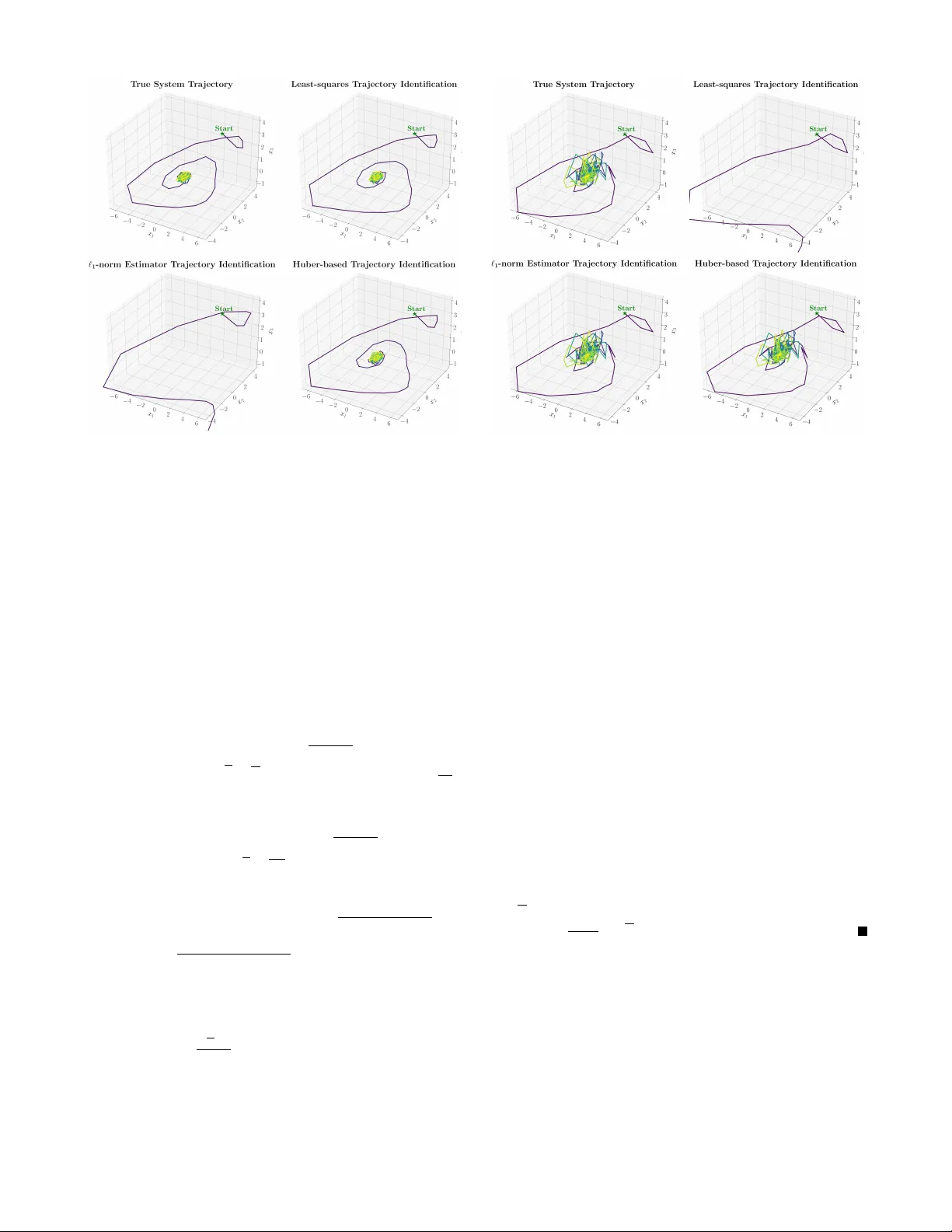
Huber -based Rob ust System Identification with Near -Optimal Guarantees Acr oss Independent and Adversarial Regimes Jihun Kim and Jav ad Lav aei Abstract — Dynamical systems can confront one of two ex- treme types of disturbances: persistent zero-mean independent noise, and sparse nonzero-mean adversarial attacks, depending on the specific scenario being modeled. While mean-based estimators like least-squares ar e well-suited for the f ormer , a median-based approach such as the ℓ 1 -norm estimator is requir ed f or the latter . In this paper , we pr opose a Huber -based estimator , characterized by a threshold constant µ , to identify the governing matrix of a linearly parameterized nonlinear system from a single trajectory of length T . This formulation bridges the gap between mean- and median-based estimation, achieving provably robust error in both extr eme disturbance scenarios under mild assumptions. In particular , for persistent zero-mean noise with a positive probability density around zero, the proposed estimator achiev es an O (1 / √ T ) error rate if the disturbance is symmetric or the basis functions are linear . For arbitrary nonzero-mean attacks that occur at each time with probability smaller than 0.5, the error is bounded by O ( µ ) . W e validate our theor etical results with experiments illustrating that integrating our approach into frameworks like SINDy yields rob ust identification of discrete-time systems. I . I N T R O D U C T I O N Modern engineering systems are inherently complex and their governing dynamics are frequently partially or fully unknown. System identification is the procedure of learning underlying models based on the state trajectory generated by the system, providing the foundation to design robust and reliable control algorithms [1]. For large-scale infrastructure such as power systems, howe ver , collecting data via forc- ing state resets often incurs massiv e operational downtime [2]. Similarly , human patients in clinical control cannot be physiologically reset [3]. Thus, practical system identification in many real-world applications necessitates learning from a single trajectory . W e formulate this task as a parameter estimation problem and consider a structured discrete-time dynamical system generating a sequence of the form x t +1 = ¯ Aϕ ( x t ) + w t , t = 0 , . . . , T − 1 , (1) where x t ∈ R n is the state, w t ∈ R n is the disturbance at time t , and T denotes the trajectory length. The system dynamics are governed by an unknown target matrix ¯ A ∈ R n × m —with rows ¯ a T 1 , . . . , ¯ a T n —and known, potentially non- linear basis functions ϕ : R n → R m chosen by the system analyst. Gi ven a single trajectory { x t } T t =0 , our objective is to accurately estimate the unknown values in ¯ A . This work was supported by the U. S. Army Research Laboratory and the U. S. Army Research Office under Grant W911NF2010219, Office of Nav al Research under Grant N000142412673, and NSF . Jihun Kim and Jav ad Lav aei are with the Department of Industrial Engineering and Opera- tions Research, Univ ersity of California, Berkeley . Emails: { jihun.kim, lavaei } @berkeley.edu The robustness of this identification problem is often challenged by the nature of disturbances { w t } T − 1 t =0 . In recent literature, two distinct disturbance regimes are often con- sidered: (a) persistent zero-mean independent noise , and (b) sparse nonzero-mean adversarial attack . The former typically arises as natural fluctuations in physical systems, commonly modeled as a non-adversarial (white) noise pro- cess present at every time [4]. In contrast, the latter appears in security and fault-diagnosis settings, where an adversary intermittently but strategically corrupts the system [5]. T o address these two extreme scenarios, recent literature has adopted two primary classes of estimators. For zero- mean independent noise, mean-based estimators such as the least-squares method ensure that persistent disturbances are av eraged out. Con versely , for zero-median sparse attacks, median-based estimators such as the ℓ 1 -norm estimator filter out any disturbances of adversarial nature. These two esti- mators correspond to the following optimization problems: min A ∈ R n × m T − 1 X t =0 ∥ x t +1 − Aϕ ( x t ) ∥ 2 2 (Least-squares) min A ∈ R n × m T − 1 X t =0 ∥ x t +1 − Aϕ ( x t ) ∥ 1 ( ℓ 1 -norm estimator) It is well-established that the least-squares method achiev es an O (1 / √ T ) error rate under persistent zero-mean independent noise with high probability after a certain finite time complexity [6], [7]. As shown in [6], this rate is indeed optimal for such a persistent noise regime. Con versely , under sparse nonzero-mean adversarial attacks, where the median of attacks is zero provided that the attack probability is smaller than 0.5, the ℓ 1 -norm estimator sho ws a funda- mentally different behavior: it achiev es exact recov ery (zero error) with high probability within finite time [8], [9]. Despite their individual efficacy , both approaches face a critical blind spot. The former approach is limited to zero- mean noise and fails against adversarial attacks, since biased disturbances do not av erage to zero. The latter approach, while robust to sparse attacks, cannot overcome persistent noise, since it requires the disturbance to be exactly zero with probability greater than 0.5. This leads to the central challenge of system identification: in practice, the underlying natur e of the disturbances is unknown in advance . Contribution. In this paper, we provide the robust system identification framew ork via the Huber estimator , using the Huber loss [10] defined by a threshold constant µ . W e estab- lish the first theoretical guarantees that the Huber estimator is universally ef fectiv e “near the best of both worlds”: 1) The Huber estimator recovers the optimal O (1 / √ T ) error rate under persistent zero-mean independent noise, when the noise has a positive probability density around zero. 2) The Huber estimator ensures that the estimation error is bounded by a constant O ( µ ) error under sparse nonzero- mean adversarial attack. Although [11] recently demonstrated the empirical ro- bustness of the Huber estimator when applied to neural networks under distinct disturbance scenarios, theoretical foundations hav e not yet been developed. W e bridge this gap by providing a rigorous analysis for the estimation of ¯ A in (1). Our framework incorporates a SINDy-type structure [12] via sufficiently expressi ve nonlinear basis functions ϕ ( x ) and a sparse target matrix ¯ A . Although the original SINDy approach relies on least-squares suited only for zero-mean noise, our work provides theoretical guarantees to handle both extreme disturbance regimes via the Huber estimator . Outline. In Section II, we outline the rele vant assumptions for each disturbance scenario. Section III formalizes the Huber estimator . Section IV presents the two main theoretical results under these scenarios, and Section V pro vides numeri- cal v alidation of our claims. The detailed proof techniques for each theorem are de veloped in Sections VI and VII. Finally , Section VIII provides concluding remarks. Notation. For a v ector x , x T is a transpose of a v ector and x ( i ) denotes its i th entry . The notation ∥ · ∥ 2 denotes the ℓ 2 - norm for vectors and the operator norm for matrices, while ∥ · ∥ 1 denotes the ℓ 1 -norm for vectors. The notation I denotes the identity matrix. Let σ ( · ) denote the sigma-algebra. E [ · ] denotes expectation and P ( · ) denotes probability . The nota- tions O ( · ) and Ω( · ) indicate an upper and a lower bound up to a positiv e constant, respectiv ely . A distribution w is symmetric if w and − w are identically distributed. I I . P R O B L E M F O R M U L A T I O N A N D C O R E A S S U M P T I O N S In this section, we state the assumptions and scenarios required to establish theoretical guarantees for the Huber es- timator . The first two assumptions ensure that the trajectories generated by the underlying true system do not diver ge. Assumption 1 (System Stability): Let ρ denote the spectral norm ∥ ¯ A ∥ 2 . Let L be a Lipschitz constant for ϕ ( · ) ; i.e., ∥ ϕ ( x ) − ϕ ( ˜ x ) ∥ 2 ≤ L ∥ x − ˜ x ∥ 2 for all x, ˜ x ∈ R n . Mor eover , ϕ (0) = 0 . The stability condition is ρL < 1 . Assumption 2 (Sub-Gaussian Disturbance): Define F t = σ { x 0 , . . . , x t } . Assume that all w t and x 0 ar e sub-Gaussian vectors 1 (not necessarily zero-mean or independent); i.e., ther e e xists σ > 0 such that ∥ x ( i ) 0 ∥ ψ 2 ≤ σ and ∥ w ( i ) t | F t ∥ ψ 2 ≤ σ for every t ≥ 0 and i ∈ { 1 , . . . , n } . Remark 1: Since Lipschitz continuity of ϕ is based on the ℓ 2 -norm, it is useful to study the ψ 2 -norm of the ℓ 2 -norm of a 1 The notion of sub-Gaussian variables is introduced in Section 2.6, [13]. A variable x is sub-Gaussian if its ψ 2 -norm ∥ x ∥ ψ 2 = inf { k > 0 : E [exp( x 2 /k 2 )] ≤ e } is finite. For example, every bounded variable is sub- Gaussian. Furthermore, a vector X ∈ R n is defined as sub-Gaussian with ψ 2 -norm σ if the scalar projection u T X is sub-Gaussian with ψ 2 -norm of at most σ for all u ∈ R n such that ∥ u ∥ 2 = 1 . sub-Gaussian variable. Assumption 2 implies that ∥∥ x 0 ∥ 2 ∥ ψ 2 and ∥∥ w t ∥ 2 ∥ ψ 2 are bounded by √ nσ . This bound is tight for a vector with independent coordinates; e.g. , when w t follows a Gaussian N (0 , σ 2 I ) , its ψ 2 -norm scales with σ and E [ ∥ w t ∥ 2 2 ] = P n i =1 E [( w ( i ) t ) 2 ] = nσ 2 , which means ∥ w t ∥ 2 concentrates around its expected value of roughly √ nσ . The next set of assumptions represents the two extreme cases of disturbances: persistent zero-mean independent noise and sparse nonzero-mean adversarial attack. Scenario 1 (P ersistent Zero-mean Independent Noise): w t is an independent, zer o-mean pr ocess for t ≥ 0 . Mor eover , E [ x 0 ] = 0 . Scenario 2 (Sparse Nonzero-mean Adversarial Attack): w t is an attack at time t with pr obability p < 0 . 5 , conditioned on F t = σ { x 0 , . . . , x t } . Mor e formally , there exists a sequence ( ξ t ) T − 1 t =0 of independent Bernoulli( p ) random variables such that { ξ t = 0 } ⊆ { w t = 0 } for all t ≥ 0 . Under this restriction on attack times, w t can be chosen arbitrarily by an adversary with access to F t at every attack time t ≥ 0 . Scenario 1 specifies that the system is under independent zero-mean noise at every time step, while Scenario 2 states that the system is under adversarial attack at each time with probability smaller than 0 . 5 . The next set of assumptions for- malize the sufficient expected excitation for each disturbance regime. Assumption 3a (Expected Excitation): Ther e exists λ > 0 such that E [ ϕ ( x t ) ϕ ( x t ) T | F t − 1 ] ⪰ λ 2 I for all t = 1 , . . . , T , meaning that ϕ ( x t ) covers entir e space in R m in expectation. Assumption 3b (Expected Excitation under Attack): Ther e exists λ > 0 such that E [ ϕ ( x t ) ϕ ( x t ) T | ξ t − 1 = 1 , F t − 1 ] ⪰ λ 2 I for all t = 1 , . . . , T , meaning that ϕ ( x t ) covers entire space in R m in expectation, whenever attack happens. Throughout the paper , we will establish theoretical guar- antees on the estimation error of the Huber estimator across both disturbance scenarios. I I I . H U B E R - BA S E D S Y S T E M I D E N T I FI C AT I O N In this section, we formalize the Huber estimator and present the underlying intuition that motiv ates its robustness. Giv en µ > 0 , consider min { a i } n i =1 T − 1 X t =0 n X i =1 H µ ( x ( i ) t +1 − a T i ϕ ( x t )) , (Huber estimator) where H µ ( z ) =      1 2 z 2 if | z | ≤ µ , µ | z | − 1 2 µ 2 if | z | > µ . (2) Note that the term x ( i ) t +1 − a T i ϕ ( x t ) is the i th entry of the residual x t +1 − Aϕ ( x t ) , where a T i denotes the i th row of A . The Huber loss (2) is con vex and acts as a quadratic penalty for small arguments and a linear penalty for large ones. The follo wing proposition formalizes ho w this dual behavior allows the Huber estimator to bridge between the least-squares and the ℓ 1 -norm estimators. Proposition 1. The pr oblem (Huber estimator) is equivalent to the pr oblem min A, { v t } t ≥ 0 T − 1 X t =0 1 2 ∥ x t +1 − Aϕ ( x t ) − v t ∥ 2 2 + µ ∥ v t ∥ 1 , (3) wher e A is a matrix whose r ows ar e a T i for i ∈ { 1 , . . . , n } . Pr oof: The joint minimization with respect to A and { v t } t ≥ 0 is equiv alent to minimizing first with respect to A , and then over { v t } t ≥ 0 . Thus, it suffices to show that min { v t } t ≥ 0 T − 1 X t =0 1 2 ∥ x t +1 − Aϕ ( x t ) − v t ∥ 2 2 + µ ∥ v t ∥ 1 = T − 1 X t =0 n X i =1 H µ ( x ( i ) t +1 − a T i ϕ ( x t )) (4) for all A . Since the left-hand side term is con vex in { v t } t ≥ 0 and can be decoupled along the time t as well as the coordinate i , the KKT optimality conditions imply that 0 ∈ − ( x ( i ) t +1 − a T i ϕ ( x t ) − v ( i ) t ) + µ∂ | v ( i ) t | , t ≥ 0 for every i ∈ { 1 , . . . , n } , where ∂ denotes the subderiv ativ e. W e consider two cases based on the KKT conditions. Case 1 : | x ( i ) t +1 − a T i ϕ ( x t ) | ≤ µ . In this case, v ( i ) t = 0 . T o see why , note that if v ( i ) t > 0 , the KKT conditions would require x ( i ) t +1 − a T i ϕ ( x t ) − v ( i ) t = µ , which incurs a contradiction. The argument for v ( i ) t < 0 follows similarly . Case 2 : | x ( i ) t +1 − a T i ϕ ( x t ) | > µ . Here, v ( i ) t  = 0 . If x ( i ) t +1 − a T i ϕ ( x t ) > µ , the KKT conditions imply v ( i ) t = x ( i ) t +1 − a T i ϕ ( x t ) − µ > 0 . Alternativ ely , if x ( i ) t +1 − a T i ϕ ( x t ) < − µ , the conditions imply v ( i ) t = x ( i ) t +1 − a T i ϕ ( x t ) + µ < 0 . Substituting the obtained v ( i ) t for ev ery t and i back into the left-hand side of (4) yields the right-hand side. This completes the proof. Remark 2: The above proposition introduces an alternativ e con vex formulation of the Huber estimator , consisting of the least-squares term P t 1 2 ∥ x t +1 − Aϕ ( x t ) − v t ∥ 2 2 and the ℓ 1 -regularization term µ P t ∥ v t ∥ 1 , which implies that the Huber estimator serves as a middle ground between the least-squares and the ℓ 1 -norm estimator . The value of µ dictates how close the Huber estimator is to either one of the two aforementioned estimators; when µ is large, the heavy penalty forces v t to zero, reducing the objectiv e nearly to the least-squares estimator giv en in (Least-squares). Conv ersely , when µ is small, v t is forced to approach the residual x t +1 − Aϕ ( x t ) to minimize the quadratic loss, effecti vely recovering the ℓ 1 -norm estimator defined in ( ℓ 1 -norm estimator). Note that µ > 0 is strictly required to ensure that (3) is well-posed; at µ = 0 , any A is optimal by choosing v t = x t +1 − Aϕ ( x t ) . In the next section, we will provide theoretical guarantees of the error rates provided by the Huber estimator . I V . M A I N R E S U L T S : N E A R T H E B E S T O F B OT H W O R L D S In this section, we provide the main results for the Huber estimator under two extreme disturbance regimes. T echnical proofs are all deferred to Sections VI and VII. The first main theorem shows that when the independent mean-zero noise is persistently injected into the system, the Huber estimator achiev es the optimal O (1 / √ T ) under an additional mild assumption on the noise. W e present the assumption and the theorem below . Assumption 4: There e xists a universal value q > 0 such that P ( | w ( i ) t | ≤ µ 2 ) ≥ q holds for every t ≥ 0 and i ∈ { 1 , . . . , n } . Theorem 1. Consider Scenario 1 and suppose that Assump- tions 1, 2, 3a, and 4 hold. Let ˆ a 1 , . . . , ˆ a n be a minimizer to (Huber estimator) , and let ¯ a T 1 , . . . , ¯ a T n be each r ow of ¯ A . Given δ ∈ (0 , 1) , when • w t has a symmetric distribution for all t ≥ 0 , or • ϕ ( x ) = ¯ B x for some ¯ B ∈ R m × n , where ∥ ¯ B ∥ 2 ≤ L , with T = Ω  n 2 L 4 σ 4 q 2 λ 4 (1 − ρL ) 4 log 2  mn δ  log  nLσ q λ (1 − ρL ) δ  , (5) it holds that ∥ ¯ a i − ˆ a i ∥ 2 = O  µ √ nLσ √ T qλ 2 (1 − ρL ) log  n δ   , ∀ i ∈ { 1 , . . . , n } with pr obability at least 1 − δ . Remark 3: This theorem demonstrates that there e xists a finite time complexity beyond which the estimation error is bounded by O ( √ n log n/ √ T ) . W e now discuss the con- ditions on the theorem beyond standard independent zero- mean noise (Scenario 1); we require (a) a positiv e probability density around zero (Assumption 4), and (b) the symmet- ric disturbance unless the system is linear . In engineering practice, process noise naturally aligns with this condition: digital quantization errors are often modeled as zero-centered uniform distrib ution [14], while thermal noise is dri ven by the aggregation of countless independent electron mov ements, which conv erges to a zero-mean Gaussian via the Central Limit Theorem [15]. Crucially , the noise in both of these standard scenarios is perfectly symmetric. Remark 4: From an analytical perspecti ve, Assumption 4 is required since the Huber estimator achieves sufficient empir- ical excitation exclusi vely via samples with small estimated errors x ( i ) t +1 − a T i ϕ ( x t ) ; the Huber loss (2) only preserves the excitation for a quadratic penalty , whereas least-squares method relies on suf ficient empirical excitation a veraged o ver all time steps. Furthermore, symmetry of disturbances is re- quired since applying the Huber penalty effecti vely truncates the estimated sample error at [ − µ, µ ] , which introduces a bias if the underlying zero-mean disturbance is asymmetric. This symmetry requirement is completely circumvented in linear systems; since linear basis functions maintain the zero-mean nature of the states x t , we can deriv e the optimal O (1 / √ T ) error rate regardless of disturbance symmetry . The second main theorem shows that the adversarial attack scenario is solved by the Huber estimator with the error bounded by O ( µ ) . Theorem 2. Consider Scenario 2 and suppose that Assump- tions 1, 2, and 3b hold. Let ˆ a 1 , . . . , ˆ a n be a minimizer to (Huber estimator) , and let ¯ a T 1 , . . . , ¯ a T n be each r ow of ¯ A . Given δ ∈ (0 , 1) , when T = Ω  ( √ nLσ ) 4 λ 4 p (1 − 2 p ) (6) × max  ( √ nLσ ) 6 log 2 ( n δ ) (1 − 2 p ) λ 6 (1 − ρL ) 2 , m log  nLσ λ (1 − ρL )   , it holds that ∥ ¯ a i − ˆ a i ∥ 2 = O  µn 2 L 4 σ 4 p (1 − 2 p ) λ 5  , ∀ i ∈ { 1 , . . . , n } with pr obability at least 1 − δ . Remark 5: This theorem demonstrates that after a finite time complexity , the Huber estimator shows a bounded error O ( µ ) . The proof uses the fact that the ℓ 1 -norm estimator indeed achiev es a zero error within finite time under Scenario 2 [8]; subsequently , we use the boundedness of the difference between the ℓ 1 -norm loss and the Huber loss. Theorems 1 and 2 elucidate the trade-of fs inv olved in selecting µ across two extreme disturbance regimes. For sparse nonzero-mean attacks, minimizing µ tightly bounds the estimation error , which is natural since small µ cor- responds to the ℓ 1 -norm estimator as noted in Remark 2. Con versely , under persistent zero-mean noise, µ must exceed a strictly positive threshold; Assumption 4 requires a positive probability density across [ − µ 2 , µ 2 ] , which is a condition im- possible to satisfy with µ = 0 for any absolutely continuous distribution. Importantly , howe ver , we do not necessarily require µ to be arbitrarily large (which corresponds to the least-squares as noted in Remark 2), but merely needs to satisfy the assumption to achiev e the optimal O (1 / √ T ) rate. Since increasing µ beyond a certain threshold does not provide benefit for persistent zero-mean noise, our theoretical results suggest a clear tuning strategy: µ should be set to the minimal value that satisfies Assumption 4 for the Huber estimator to pro vide the optimal defense against both extreme disturbance scenarios. V . N U M E R I C A L E X P E R I M E N T S In this section, we provide experimental validations tested on the discrete-time dynamical systems. For pictorial illustra- tion, we consider three-dimensional x = [ x 1 , x 2 , x 3 ] T ∈ R 3 . ϕ ( x ) = [ x 1 , x 2 , x 3 ,x 1 x 2 , x 2 x 3 , x 3 x 1 , x 2 1 , x 2 2 , x 2 3 , sin( x 1 x 2 ) , cos( x 3 )] T ∈ R 11 with ¯ A =   0 . 8 − 0 . 5 0 0 0 . 4 0 0 0 0 0 . 1 0 0 . 5 0 . 8 0 0 . 06 0 0 − 0 . 05 0 0 0 0 0 0 0 . 45 0 0 0 . 05 0 0 0 0 0 . 1   , (a) Persistent zero-mean noise (b) Sparse nonzero-mean attack Fig. 1: Estimation error over T rajectory Length which is designed to be sparse in an expressiv e nonlinear feature space ϕ ( x ) to incorporate the SINDy frame work [12]. The true trajectory of the system is generated from x 0 = [3 , 3 , 3] T . x t +1 = ¯ Aϕ ( x t ) + w t , t = 0 , . . . , T − 1 , where T = 2500 . W e consider two disturbance scenarios for w t ∈ R 3 : (a) a symmetric case where each component is independently uniform on [ − 0 . 2 , 0 . 2] , and (b) a sparse case where w t equals the zero vector with probability 0 . 6 , and with probability 0 . 4 , its components are uniformly distributed on [0 . 2 − min {∥ x t ∥ 2 , 1 } , 0 . 2 + min {∥ x t ∥ 2 , 1 } ] , deliberately designed to depend on x t . Under each of these disturbances, we run (Least-squares), ( ℓ 1 -norm estimator), and (Huber estimator) with µ = 0 . 1 to obtain estimates ˆ A . Figure 1 validates the theoretical error bounds deri ved in Theorems 1 and 2 by plotting the Frobenius error norm ∥ ¯ A − ˆ A ∥ F , against the trajectory length T ∈ [40 , 2500] . Under persistent zero-mean noise (Figure 1(a)), the least- squares estimator con verges at a rate of O (1 / √ T ) , with the Huber estimator matching this rate up to a constant factor . Under sparse nonzero-mean attack (Figure 1(b)), the ℓ 1 -norm estimator perfectly recovers the system with zero error for T ≥ 100 . The Huber estimator yields a bounded constant error of O ( µ ) , significantly outperforming the least-squares approach. Ultimately , these results confirm that the Huber estimator serves as a robust bridge between standard mean- and median-based estimators. W e also inv estigate the stability of the true and recon- structed trajectories. Figures 2 and 3 each display four trajectories: the true system path and those reconstructed by the three estimators at T = 2500 , with a “Start” marker and time-based coloring. Under persistent zero-mean noise in Figure 2, the true trajectory is stable; the least-squares and Huber estimators both successfully reconstruct stable paths that closely track the truth, whereas the ℓ 1 -norm estimate fails to stabilize. Con versely , under sparse nonzero-mean attack in Figure 3, the ℓ 1 -norm estimator achieves a perfect reconstruction of the true stable trajectory , while the least- squares estimate diver ges. The Huber estimator, howe ver , continues to successfully produce a stable trajectory that approximates the truth. This demonstrates that the Huber- based estimator, with an appropriate value for µ , reliably achiev es accurate reconstruction under both extreme distur- bance scenarios. Fig. 2: Stability of trajectories reconstructed based on differ - ent estimators: Persistent zero-mean independent noise V I . P R O O F O F T H E O R E M 1 In this section, we prov e Theorem 1, which shows the efficac y of the Huber estimator under Scenario 1. W e begin by presenting a useful lemma on vector -v alued martingales from [16]. Lemma 1 ([16]). Consider a filtration A − 1 ⊂ A 0 ⊂ . . . and a vector -valued martingale differ ence sequence { ξ t } t ≥ 0 adapted to {A t } ; i.e., E [ ξ t | A t − 1 ] = 0 , ξ t is A t -measurable and square-inte grable for all t ≥ 0 . Let κ = 1 if { ξ t } ⊂ R m and κ = 1 + 2 log m if { ξ t } ⊂ R m × m ar e symmetric. 1) Let σ t ≥ 0 satisfy E [exp( ∥ ξ t ∥ 2 2 /σ 2 t ) | A t − 1 ] ≤ e . Then, P     T − 1 X t =0 ξ t    2 ≥ √ 2( √ κ + s ) v u u t T − 1 X t =0 σ 2 t  ≤ exp  − s 2 3  . 2) Let σ t ≥ 0 satisfy E [exp( ∥ ξ t ∥ 2 /σ t ) | A t − 1 ] ≤ e . Then, P     T − 1 X t =0 ξ t    2 ≥ √ 2( √ eκ + s ) v u u t T − 1 X t =0 σ 2 t  ≤ 2 exp  − min { s 2 , 16 τ s } 64  , wher e τ = ∥ ( σ 0 ,...,σ T − 1 ) ∥ 2 max t ∈{ 0 ,...,T − 1 } | σ t | . The next lemma bounds the ψ 2 -norm of ∥ ϕ ( x t ) ∥ 2 for all t ≥ 0 . Lemma 2. Under Assumptions 1 and 2, we have   ∥ ϕ ( x t ) ∥ 2   ψ 2 ≤ √ nLσ 1 − ρL for every t = 0 , . . . , T − 1 . Pr oof: For k = 0 , 1 , . . . , define the sequence { x k t } as the state trajectory generated from x k 0 = x 0 , x k t +1 = ¯ Aϕ ( x k t ) + w k t , t = 0 , . . . , T − 1 , Fig. 3: Stability of trajectories reconstructed based on differ - ent estimators: Sparse nonzero-mean adversarial attack where w k t is the truncated noise defined as w t for t < k and equals zero otherwise. For notational simplicity , let x − 1 t = 0 for all t ≥ 0 . Noting that x t t = x t , we can then establish that ∥ ϕ ( x t ) ∥ 2 =     t X j =0  ϕ ( x j t ) − ϕ ( x j − 1 t )      2 ≤ t X j =0 ∥ ϕ ( x j t ) − ϕ ( x j − 1 t ) ∥ 2 ≤ t X j =0 L ∥ x j t − x j − 1 t ∥ 2 ≤ L ( ρL ) t ∥ x 0 ∥ 2 + L t X j =1 ( ρL ) t − j ∥ w j − 1 ∥ 2 , (7) where the last inequality comes from ∥ x j t − x j − 1 t ∥ 2 ≤ ( ρL ) t − j ∥ w j − 1 ∥ 2 since x j t − x j − 1 t = ( ¯ Aϕ ) t − j  ¯ Aϕ ( . . . ¯ Aϕ ( x 0 ) + w 0 . . . ) + w j − 1  − ( ¯ Aϕ ) t − j  ¯ Aϕ ( . . . ¯ Aϕ ( x 0 ) + w 0 . . . ) + 0  . (8) Similarly , we hav e x 0 t = ( ¯ Aϕ ) t ( x 0 ) , which implies that ∥ x 0 t ∥ 2 ≤ ( ρL ) t ∥ x 0 ∥ 2 . W e substitute upper bounds on each ψ 2 -norm (see Remark 1 that ∥ x 0 ∥ 2 , ∥ w j − 1 ∥ 2 hav e ψ 2 -norm of √ nσ ), and use the geometric sum to conclude that (7) is bounded by L 1 − ρL · √ nσ . The next lemma shows that either symmetric disturbances with nonlinear basis functions or generic zero-mean distur- bances in linear systems provide tractable theoretical bounds. Lemma 3. Define H ′ µ ( z ) =      z , if | z | ≤ µ µ, if z > µ , − µ, if z < − µ , (9) which is the first derivative of the Huber function H µ ( z ) . Consider Scenario 1 and suppose that Assumptions 1, 2, and 4 hold. Given δ ∈ (0 , 1) , when • w t has a symmetric distribution for all t ≥ 0 , or • ϕ ( x ) = ¯ B x for some ¯ B ∈ R m × n , where ∥ ¯ B ∥ 2 ≤ L , the bound      T − 1 X t =0 H ′ µ ( w ( i ) t ) ϕ ( x t )      2 = O  √ T µ √ nLσ 1 − ρL log  1 δ   holds with pr obability at least 1 − δ . Pr oof: By the triangle inequality , we hav e      T − 1 X t =0 H ′ µ ( w ( i ) t ) ϕ ( x t )      2 ≤      T − 1 X t =0 E [ H ′ µ ( w ( i ) t )] ϕ ( x t )      2 | {z } ( A ) +      T − 1 X t =0  H ′ µ ( w ( i ) t ) − E [ H ′ µ ( w ( i ) t )]  ϕ ( x t )      2 . | {z } ( B ) W e now separately analyze each term. T erm (A)— Case 1 : In the case where w t is symmetric, we have E [ H ′ µ ( w ( i ) t )] = 0 for all t ≥ 0 , regardless of the value of µ , which implies that T erm ( A ) = 0 . T erm (A)— Case 2 : W e now consider the case where ϕ ( x ) is linear in x ; i.e. , ϕ ( x ) = ¯ B x . For notational simplicity , let w − 1 = x 0 . Recalling the definition of { x k t } in the proof of Lemma 2, we rewrite the term as T erm ( A ) =      T − 1 X t =0 E [ H ′ µ ( w ( i ) t )] t X j =0  ϕ ( x j t ) − ϕ ( x j − 1 t )       2 =      T − 1 X j =0 T − 1 X t = j E [ H ′ µ ( w ( i ) t )] · ¯ B ( ¯ A ¯ B ) t − j w j − 1      2 , (10) by considering (8) in the linear case and interchanging the order of summation. Define a filtration with inv erse order G j = σ { w T − 1 , w T − 2 , . . . , w j } . The term P T − 1 t = j E [ H ′ µ ( w ( i ) t )] · ¯ B ( ¯ A ¯ B ) t − j w j − 1 is mean zero giv en G j (since E [ w j − 1 | G j ] = E [ w j − 1 ] = 0 ), and G j − 1 - measurable. Moreover ,          T − 1 X t = j E [ H ′ µ ( w ( i ) t )] · ¯ B ( ¯ A ¯ B ) t − j w j − 1     2     G j      ψ 2 ≤ T − 1 X t = j µ ∥ ¯ B ( ¯ A ¯ B ) t − j ∥ 2 ·   ∥ w j − 1 ∥ 2   ψ 2 ≤ µL · √ nσ 1 − ρL holds since | E [ H ′ µ ( w ( i ) t )] | ≤ µ , and apply geometric sum similar to the deriv ation of Lemma 2. By applying the first property of Lemma 1, there exists c 1 > 0 such that P      T − 1 X j =0 T − 1 X t = j E [ H ′ µ ( w ( i ) t )] · ¯ B ( ¯ A ¯ B ) t − j w j − 1     2 ≥ c 1 (1 + s ) √ T µL √ nσ 1 − ρL  ≤ exp  − s 2 3  This implies that T erm ( A ) = O  √ T µ √ nLσ 1 − ρL r log  1 δ   (11) holds with probability at least 1 − δ 3 . T erm (B): For this term, we note that ( H ′ µ ( w ( i ) t ) − E [ H ′ µ ( w ( i ) t )]) ϕ ( x t ) is F t +1 -measurable and is a mean-zero variable giv en F t (since ϕ ( x t ) is F t -measurable). W e also hav e   ∥ ( H ′ µ ( w ( i ) t ) − E [ H ′ µ ( w ( i ) t )]) ϕ ( x t ) ∥ 2   F t   ψ 2 = O  µ ∥ ϕ ( x t ) ∥ 2  , since | H ′ µ ( w ( i ) t ) − E [ H ′ µ ( w ( i ) t )] | ≤ 2 µ . Then, applying the first property of Lemma 1, there exists c 2 > 0 such that P     T − 1 X t =0  H ′ µ ( w ( i ) t ) − E [ H ′ µ ( w ( i ) t )]  ϕ ( x t )     2 ≥ c 2 (1 + s ) v u u t T − 1 X t =0 µ 2 ∥ ϕ ( x t ) ∥ 2 2 ! ≤ exp  − s 2 3  (12) Note that V := P T − 1 t =0 ∥ ϕ ( x t ) ∥ 2 2 is a sub-e xponential variable with ψ 1 -norm 2 T  √ nLσ 1 − ρL  2 , since we can apply Lemma 2 to ∥ V ∥ ψ 1 ≤ P T − 1 t =0 ∥∥ ϕ ( x t ) ∥ 2 2 ∥ ψ 1 . Thus, there exists a constant c 3 > 0 such that V < V max holds with probability at least 1 − δ 3 , where V max := c 3 T  √ nLσ 1 − ρL  2 log  1 δ  . Under the ev ent that V < V max , (12) implies that T erm ( B ) = O  µ p V max r log  1 δ   = O  √ T µ √ nLσ 1 − ρL log  1 δ  (13) holds with probability at least 1 − δ 3 . Note that an upper bound on T erm ( B ) gi ven in (13) dominates both cases for T erm ( A ) in order . W e complete the proof by applying the union bound over { V < V max } , (13), and include (11) in (A)- Case 2 . The next lemma establishes that suf ficient expected ex- citation implies sufficient empirical excitation with high probability . Lemma 4. Suppose that Assumptions 1, 2, and 3a hold. Consider a subset of { 1 , . . . , T } to be T and its cardinality as |T | . Given δ ∈ (0 , 1) , when |T | = Ω  ( √ nLσ ) 4 λ 4 (1 − ρL ) 2 log  m δ  log  1 δ   , (14) we have P t ∈T ϕ ( x t ) ϕ ( x t ) T ⪰ λ 2 I 2 |T | with pr obability at least 1 − δ . 2 For a sub-Gaussian variable x with ψ 2 -norm σ , x 2 is a sub-exponential variable with ψ 1 -norm ∥ x 2 ∥ ψ 1 = ∥ x ∥ 2 ψ 2 = σ 2 . The notion of sub- exponential variables are introduced in Section 2.8, [13]. Pr oof: By Assumption 3a, we have P t ∈T E [ ϕ ( x t ) ϕ ( x t ) T | F t − 1 ] ⪰ |T | λ 2 I . T o arrive at the conclusion, it suffices to prove that     X t ∈T ϕ ( x t ) ϕ ( x t ) T − E [ ϕ ( x t ) ϕ ( x t ) T | F t − 1 ]     2 ≤ |T | λ 2 2 holds with probability at least 1 − δ . Now , define ˜ x t = x t − w t − 1 = ¯ Aϕ ( x t − 1 ) and consider the separation ϕ ( x t ) = ϕ ( ˜ x t ) + E [ ϕ ( x t ) − ϕ ( ˜ x t ) | F t − 1 ] | {z } A t + ϕ ( x t ) − ϕ ( ˜ x t ) − E [ ϕ ( x t ) − ϕ ( ˜ x t ) | F t − 1 ] | {z } B t . Noting that the term A t is F t − 1 -measurable, and the term B t has mean zero giv en F t − 1 , we have ϕ ( x t ) ϕ ( x t ) T − E [ ϕ ( x t ) ϕ ( x t ) T | F t − 1 ] = A t B T t + B t A T t | {z } C t + B t B T t − E [ B t B T t | F t − 1 ] | {z } D t . Thus, we need to bound ∥ P t ∈T C t + D t ∥ 2 . T o this end, we will separately bound ∥ P t ∈T C t ∥ 2 and ∥ P t ∈T D t ∥ 2 . Note that both C t and D t are F t -measurable and mean-zero giv en F t − 1 . First, noting that ∥ C t ∥ 2 ≤ 2 ∥ A t ∥ 2 ∥ B t ∥ 2 , we have   ∥ C t ∥ 2   F t − 1   ψ 2 ≤ 2 ∥ A t ∥ 2 ·   ∥ B t ∥ 2   F t − 1   ψ 2 ≤ 2 ∥ A t ∥ 2 · 2 L   ∥ w t − 1 ∥ 2   ψ 2 ≤ 4 ∥ A t ∥ 2 · L √ nσ, since ∥ ϕ ( x t ) − ϕ ( ˜ x t ) ∥ 2 ≤ L ∥ x t − ˜ x t ∥ 2 = L ∥ w t − 1 ∥ 2 . (15) By applying the first property of Lemma 1, there exists c 4 > 0 such that P     X t ∈T C t    2 ≥ c 4 ( p 1 + log m + s ) s X t ∈T ( √ nLσ ) 2 ∥ A t ∥ 2 2  ≤ exp  − s 2 3  . (16) Note that W := P t ∈T ∥ A t ∥ 2 2 is a sub-exponential variable with ψ 1 -norm |T |  2 √ nLσ 1 − ρL  2 (since ∥ ϕ ( ˜ x t ) ∥ 2 and E [ ∥ ϕ ( x t ) − ϕ ( ˜ x t ) ∥ 2 | F t − 1 ] both have ψ 2 -norm of at most √ nLσ 1 − ρL ). Thus, there exists a constant c 5 > 0 such that W < W max holds with probability at least 1 − δ 3 , where W max := c 5 |T |  √ nLσ 1 − ρL  2 log  1 δ  . Under the ev ent W < W max , (16) implies that    X t ∈T C t    2 = O   p log m + r log  1 δ  p |T | ( √ nLσ ) 2 1 − ρL r log  1 δ   (17) with probability at least 1 − δ 3 . Second, noting that ∥ B t B T t ∥ 2 = ∥ B t ∥ 2 2 , we have   ∥ D t ∥ 2 | F t − 1   ψ 1 ≤ 2   ∥ B t ∥ 2 2 | F t − 1   ψ 1 ≤ 2   (2 L ∥ w t − 1 ∥ 2 ) 2   ψ 1 = 2   2 L ∥ w t − 1 ∥ 2   2 ψ 2 ≤ 8( √ nLσ ) 2 , where the second inequality follows from (15). From the second property of Lemma 1, there exists c 6 > 0 such that P     X t ∈T D t    2 ≥ c 6 ( p 1 + log m + s ) p |T | ( √ nLσ ) 2  ≤ 2 exp  − min { s 2 , 16 p |T | s } 64  . This implies that    X t ∈T D t    2 = O   p log m + log  1 δ  p |T | ( √ nLσ ) 2  (18) with probability at least 1 − δ 3 . Since (17) dominates (18),   P t ∈T C t + D t   2 is bounded by (17) with probability at least 1 − δ , by constructing the union bound over { W < W max } , (17), and (18). For (17) to be bounded by |T | λ 2 2 , it suffices for |T | to satisfy (14). This completes the proof. Now , we are finally ready to prov e our main theorem that validates that the Huber estimator obtains O (1 / √ T ) error under persistent zero-mean independent noise process. Proof of Theorem 1 : Since H µ is con ve x, the first-order conditions provide necessary and sufficient conditions for optimality of (Huber estimator). Then, considering that x ( i ) t +1 = ¯ a T i ϕ ( x t ) + w ( i ) t , and denoting ¯ ϵ i = ¯ a i − ˆ a i for each i , we have T − 1 X t =0 H ′ µ (¯ ϵ T i ϕ ( x t ) + w ( i ) t ) · ϕ ( x t ) = 0 , ∀ i ∈ { 1 , . . . , n } , (19) where H ′ µ ( z ) is defined in (9). Let F ( i ) ( ϵ ) := T − 1 X t =0 H ′ µ ( ϵ T ϕ ( x t ) + w ( i ) t ) · ϕ ( x t ) . W e define the following time index set S i ( ϵ ) = { t ∈ { 0 , . . . , T − 1 } : | ϵ T ϕ ( x t ) + w ( i ) t | ≤ µ } . Then, the Jacobian of F ( i ) ( ϵ ) is defined as J ( i ) ( ϵ ) = P t ∈ S i ( ϵ ) ϕ ( x t ) ϕ ( x t ) T , since the second deriv ati ve of H µ ( z ) is 1 if | z | ≤ µ and 0 otherwise. By the fundamental theorem of calculus, we hav e F ( i ) ( ϵ ) − F ( i ) (0) = Z 1 0 J ( i ) ( sϵ ) ϵ ds. (20) Let Γ i = { t ∈ { 0 , . . . , T − 1 } : | w ( i ) t | ≤ µ 2 } . W e now consider the ev ents E 1 = n | Γ i | ≥ q T 2 o , E 2 =  | ϵ T ϕ ( x t ) | ≤ µ 2 , ∀ t = 0 , . . . , T − 1  Under these two ev ents, we know that there exists a time index set ˜ Γ i ( ϵ ) with a cardinality of at least q T 2 , such that for all t ∈ ˜ Γ i ( ϵ ) , | w ( i ) t | ≤ µ 2 and | ϵ T ϕ ( x t ) | ≤ µ 2 . More importantly , ˜ Γ i ( ϵ ) is a subset of S i ( sϵ ) for any 0 ≤ s ≤ 1 . Then, we consider the third ev ent E 3 = n X t ∈ ˜ Γ i ( ϵ ) ϕ ( x t ) ϕ ( x t ) T ⪰ λ 2 I 2 · q T 2 o . Under this event, we know that J ( i ) ( sϵ ) ⪰ λ 2 q T 4 I for any 0 ≤ s ≤ 1 . By multiplying ϵ T to both sides of (20), we obtain ϵ T F ( i ) ( ϵ ) − ϵ T F ( i ) (0) = Z 1 0 ϵ T J ( i ) ( sϵ ) ϵ ds ≥ Z 1 0 λ 2 q T 4 ∥ ϵ ∥ 2 2 ds = λ 2 q T 4 ∥ ϵ ∥ 2 2 . (21) Now , we will measure the probability that the events E 1 , E 2 , E 3 hold simultaneously . For E 1 , one can apply the Chernoff bound under Assumption 4 to obtain P ( | Γ i | ≥ q T 2 ) ≥ 1 − exp( − q T 8 ) , which implies that T = Ω  1 q log( 1 δ )  ensures that P ( E 1 ) ≥ 1 − δ 6 . For E 2 , we construct a union bound ov er all t to obtain max t ∈{ 0 ,...,T − 1 } ∥ ϕ ( x t ) ∥ 2 = O  √ nLσ 1 − ρL q log( T δ )  as P  max t ∈{ 0 ,...,T − 1 } ∥ ϕ ( x t ) ∥ 2 ≥ s  = P  {∥ ϕ ( x 0 ) ∥ 2 ≥ s } ∪ · · · ∪ {∥ ϕ ( x T − 1 ) ∥ 2 ≥ s }  ≤ T · 2 exp  − Ω  s 2 ( √ nLσ / (1 − ρL )) 2  , for all s ≥ 0 . Considering that | ϵ T ϕ ( x t ) | ≤ ∥ ϵ ∥ 2 ∥ ϕ ( x t ) ∥ 2 , there exists a constant c 7 > 0 such that ∥ ϵ ∥ 2 ≤ c 7 µ (1 − ρL ) √ nLσ p log( T /δ ) := R = ⇒ P ( E 2 ) ≥ 1 − δ 6 . For E 3 , since | ˜ Γ i ( ϵ ) | ≥ q T 2 under E 1 ∩ E 2 , when q T 2 satisfies the time complexity (14), E 3 holds with probability at least 1 − δ 6 . T aking the union bound, when ∥ ϵ ∥ 2 ≤ R and q T 2 satisfies the time complexity (14) (which already subsumes T = Ω( 1 q log( 1 δ )) ), we hav e P ( E 1 ∩ E 2 ∩ E 3 ) ≥ 1 − δ 2 ; as a result, (21) holds with probability at least 1 − δ 2 . Meanwhile, ∥ F ( i ) (0) ∥ 2 is bounded by O ( √ T ) with prob- ability at least 1 − δ 2 , which follows from Lemma 3. In this case, large enough T ensures that λ 2 q T 4 R − ∥ F ( i ) (0) ∥ 2 > 0 . In particular , using the fact that T ≥ 2 A log( A/δ ) implies T log( T /δ ) > A , it suffices to hav e T = Ω  ( √ nLσ ) 4 q 2 λ 4 (1 − ρL ) 4 log 2  m δ  log  Lnσ q λ (1 − ρL ) δ  (22) for λ 2 q T 4 R − ∥ F ( i ) (0) ∥ 2 > 0 to hold with probability at least 1 − δ 2 . In such a case, as a by-product, we hav e R = O  µ √ nLσ √ T q λ 2 (1 − ρL ) log  1 δ  . Note that (22) implies that q T 2 satisfies the time complexity (14). Thus, we can use the union bound to establish that ∥ ϵ ∥ 2 = R in (21) implies that ϵ T F ( i ) ( ϵ ) ≥ λ 2 q T 4 ∥ ϵ ∥ 2 2 − ∥ ϵ ∥ 2 ∥ F ( i ) (0) ∥ 2 = R  λ 2 q T 4 R − ∥ F ( i ) (0) ∥ 2  > 0 . (23) with probability at least 1 − δ under (22). Note that ¯ ϵ i defined in (19) cannot satisfy (23) since F ( i ) (¯ ϵ i ) = 0 . Meanwhile, by the continuity of F ( i ) ( ϵ ) , ∥ ϵ ∥ 2 = R ⇒ ϵ T F ( i ) ( ϵ ) > 0 implies that there exists ∥ ϵ ∥ 2 < R such that F ( i ) ( ϵ ) = 0 (see Theorem 6.3.4, [17]). Noting that a set of optimal points to con vex optimization problem (Huber estimator) is indeed conv ex, every solution to (Huber estimator) should satisfy that ∥ ϵ ∥ 2 < R . Under (22), we have ∥ ϵ ∥ 2 < R = O  µ √ nLσ √ T qλ 2 (1 − ρL ) log  1 δ   (24) with probability at least 1 − δ . T o ensure that the aforementioned argument holds for all i ∈ { 1 , . . . , n } , we substitute δ n for δ in (22) and (24) to complete the proof. ■ V I I . P R O O F O F T H E O R E M 2 In this section, we pro ve Theorem 2, which establishes that the estimation error of the Huber estimator is strictly bounded by a constant under Scenario 2. The follo wing lemma sho ws that the ℓ 1 -norm estimator perfectly recov ers the system with high probability . Lemma 5. Consider Scenario 2 and suppose that Assump- tions 1, 2, and 3b hold. Let f ( i ) ( a i ) := P T − 1 t =0 | x ( i ) t +1 − a T i ϕ ( x t ) | . Given δ ∈ (0 , 1) , when T satisfies (6) , ther e exists a constant c > 0 such that f ( i ) ( a i ) − f ( i ) (¯ a i ) ≥ cT · p (1 − 2 p ) λ 5 n 2 L 4 σ 4 ∥ a i − ¯ a i ∥ 2 , ∀ a i ∈ R m , ∀ i ∈ { 1 , . . . , n } with pr obability at least 1 − δ . As a by-pr oduct, ¯ A is the unique global solution to ( ℓ 1 -norm estimator) with pr obabil- ity at least 1 − δ . Pr oof: Letting u := ¯ a i − a i ∥ ¯ a i − a i ∥ 2 ∈ R m , we have f ( i ) ( a i ) − f ( i ) (¯ a i ) = T − 1 X t =0 | (¯ a i − a i ) T ϕ ( x t ) + w ( i ) t | − | w ( i ) t | ≥ T − 1 X t =0 , w ( i ) t =0 | (¯ a i − a i ) T ϕ ( x t ) | + T − 1 X t =0 , w ( i ) t  =0 (¯ a i − a i ) T ϕ ( x t )sgn( w ( i ) t ) = ∥ ¯ a i − a i ∥ 2  T − 1 X t =0 , w ( i ) t =0 | u T ϕ ( x t ) | + T − 1 X t =0 , w ( i ) t  =0 u T ϕ ( x t )sgn( w ( i ) t )  , where the first inequality follo ws from the gradient inequality for a conv ex function | · | and its subgradient being a sign function. T o univ ersally lower bound this expression over ∥ u ∥ 2 = 1 , it suffices to study a lower bound on inf ∥ u ∥ 2 =1 T − 1 X t =0 , w ( i ) t =0 | u T ϕ ( x t ) | | {z } ( A ) −      T − 1 X t =0 , w ( i ) t  =0 ϕ ( x t ) · sgn( w ( i ) t )      2 | {z } ( B ) . Moreov er , an additional lower bound can be established by letting ξ t ∼ Bernoulli(2 p ) (see Scenario 2) independently ov er t , while letting P (sgn( w ( i ) t ) > 0) = P (sgn( w ( i ) t ) < 0) whenev er the attack occurs (see Theorem 3, [8]). Thus, we will study the two terms under this sign-symmetric disturbance structure. T erm (A): This term is related to the time index in the absence of attack. Howe ver , sufficient excitation is inevitable to lower bound this term; thus, to take advantage of As- sumption 3b, we consider the time index set T non := { t ∈ { 1 , . . . , T − 1 } : w ( i ) t = 0 , ξ t − 1 = 1 } . For each t ∈ T non , we have for a fixed ∥ u ∥ 2 = 1 that P  | u T ϕ ( x t ) | ≥ λ 2    F t − 1  ≥ λ 4 ( √ nLσ ) 4 , (25) which adapts Lemma 3 in [18]. Note that additional n 2 factor is introduced compared to [18] since they assumed ∥∥ w t ∥ 2 ∥ ψ 2 ≤ σ , while our standard assumption on sub- Gaussian disturbances implies ∥∥ w t ∥ 2 ∥ ψ 2 ≤ √ nσ (see Re- mark 1). Define Y t := λ 2 I {| u T ϕ ( x t ) | ≥ λ 2 } , where I {·} de- notes the indicator function, which satisfies | u T ϕ ( x t ) | ≥ Y t for all t . Since Y t − E [ Y t | F t − 1 ] forms a Martingale difference sequence, we use the Chernoff bound on martingales to (25) to obtain P  X t ∈T non Y t ≤ | T non | λ 5 4( √ nLσ ) 4  ≤ exp  − | T non | λ 4 8( √ nLσ ) 4  . Since | u T ϕ ( x t ) | ≥ Y t , we have |T non | = Ω  ( √ nLσ ) 4 λ 4 log  1 δ  = ⇒ P  X t ∈T non | u T ϕ ( x t ) | ≥ | T non | λ 5 4( √ nLσ ) 4  ≥ 1 − δ 4 . (26) Moreov er , we hav e P t ∈|T non | ∥ ϕ ( x t ) ∥ 2 has ψ 2 -norm of |T non | ( √ nLσ 1 − ρL ) . Given ϵ > 0 , when ∥ u − ˜ u ∥ 2 ≤ ϵ , we have     X t ∈T non | u T ϕ ( x t ) | − X t ∈T non | ˜ u T ϕ ( x t ) |     = O  ϵ |T non |  √ nLσ 1 − ρL  log  1 δ  (27) with probability at least 1 − δ 4 . Let ϵ = O  λ 5 (1 − ρL ) ( √ nLσ ) 5 log(1 /δ )  to bound (27) by |T non | λ 5 8( √ nLσ ) 4 . By covering number arguments (see Corollary 4.2.11, [13]), we can construct an ϵ -net of at most (1 + 2 ϵ ) m for the vectors u that simultaneously satisfy P t ∈T non | u T ϕ ( x t ) | ≥ |T non | λ 5 4( √ nLσ ) 4 with probability at least 1 − δ 4 , which is attained by replacing δ in (26) with δ (1+ 2 ϵ ) m , which requires |T non | = Ω  ( √ nLσ ) 4 λ 4 h m log  nLσ λ (1 − ρL )  + log  1 δ i . (28) Under (28), we can take a union bound over this net and (27) to guarantee T erm (A) ≥ inf ∥ u ∥ 2 =1 X t ∈T non | u T ϕ ( x t ) | ≥ |T non | λ 5 8( √ nLσ ) 4 (29) with probability at least 1 − δ 2 . T erm (B): This term is related to the time index under attack. Define T att := { t ∈ { 0 , . . . , T − 1 } : w ( i ) t  = 0 } . Bounding this term is similar to the approach to bound T erm (B) in the proof of Lemma 3. Since | sgn( w ( i ) t ) | ≤ 1 , we have   ∥ sgn( w ( i ) t ) ϕ ( x t ) ∥ 2   F t   ψ 2 = O  ∥ ϕ ( x t ) ∥ 2  , Considering that E [sgn( w ( i ) t )] = 0 , we apply the similar technique used for (12) and (13), except that µ and T are now replaced with 1 and |T att | , respectiv ely . Thus, we have T erm (B) = O  p |T att | √ nLσ 1 − ρL log  1 δ  (30) with probability at least 1 − δ 4 . Using the Chernoff bound to { ξ t } t ≥ 0 , when T = Ω  1 p (1 − 2 p ) log  1 δ  , we have |T non | ≥ p (1 − 2 p ) T , |T att | ≤ 4 pT (31) with probability at least 1 − δ 4 . W e construct the union bound ov er (29), (30), and (31) to have T erm (A) − T erm (B) = Ω( p (1 − 2 p ) T λ 5 ( √ nLσ ) 4 ) with probability at least 1 − δ when the time complexity satisfies both (28) and T = Ω  ( √ nLσ ) 10 p (1 − 2 p ) 2 λ 10 (1 − ρL ) 2 log 2  1 δ   . (32) T o ensure that the aforementioned argument holds for all i ∈ { 1 , . . . , n } , we substitute δ n for δ in (28) and (32) to obtain the time (6). This completes the proof. W e no w prove that the estimation error of the Huber estimator is bounded by O ( µ ) under sparse nonzero-mean adversarial attacks. Proof of Theorem 2 : Let f ( i ) ( a i ) := P T − 1 t =0 | x ( i ) t +1 − a T i ϕ ( x t ) | and h ( i ) ( a i ) := P T − 1 t =0 H µ ( x ( i ) t +1 − a T i ϕ ( x t )) . Note that we hav e µ | z | − H µ ( z ) =      µ | z | − 1 2 z 2 if | z | ≤ µ , 1 2 µ 2 if | z | > µ , where 0 ≤ µ | z | − 1 2 z 2 ≤ 1 2 µ 2 if | z | ≤ µ . This implies that 0 ≤ µf ( i ) ( a i ) − h ( i ) ( a i ) ≤ µ 2 T 2 , ∀ a i ∈ R m . Then, for ev ery i ∈ { 1 , . . . , n } , we obtain the relationship µf ( i ) (ˆ a i ) ≤ h ( i ) (ˆ a i ) + µ 2 T 2 ≤ h ( i ) (¯ a i ) + µ 2 T 2 ≤ µf ( i ) (¯ a i ) + µ 2 T 2 , where the second inequality follows from the optimality of ˆ a i to (Huber estimator) for e very i . This quantifies an upper bound on µf ( i ) (ˆ a i ) − µf ( i ) (¯ a i ) . Lemma 5 implies that under (6), there exists a constant c > 0 such that cµT p (1 − 2 p ) λ 5 n 2 L 4 σ 4 ∥ ˆ a i − ¯ a i ∥ 2 ≤ µf ( i ) (ˆ a i ) − µf ( i ) (¯ a i ) ≤ µ 2 T 2 for all i , with probability at least 1 − δ . Rearranging the left-hand and right-hand sides completes the proof. ■ V I I I . C O N C L U S I O N In this paper , we introduce a robust system identification framew ork based on the Huber estimator, a principled middle ground between the least-squares and the ℓ 1 -norm estimators. W e prove that, giv en a positiv e noise density around zero, the Huber estimator achie ves the optimal O (1 / √ T ) error rate when the disturbances are symmetric or the basis functions are linear . Furthermore, we establish a bounded constant estimation error against sparse adversarial attacks. This work provides the first unified theoretical guarantees for the Huber estimator across both extreme disturbance regimes. R E F E R E N C E S [1] L. Ljung, System Identification, Theory for the User , 2nd ed. Upper Saddle River , NJ: Prentice Hall, 1998. [2] A. Ghodeswar, M. Bhandari, and B. Hedman, “Quantifying the eco- nomic costs of power outages owing to extreme events: A systematic revie w , ” Renewable and Sustainable Energy Reviews , vol. 207, 2025. [3] A. Allam, S. Feuerriegel, M. Rebhan, and M. Krauthammer, “ An- alyzing patient trajectories with artificial intelligence, ” Journal of Medical Internet Resear ch , vol. 23, no. 12, e29812, 2021. [4] M. I. Freidlin and A. D. W entzell, Random P erturbations of Dy- namical Systems (Grundlehren der mathematischen W issenschaften), 3rd ed. Ne w Y ork, NY: Springer, 2012, vol. 260. [5] A. T eixeira, I. Shames, H. Sandberg, and K. H. Johansson, “A secure control framework for resource-limited adversaries, ” Automatica , vol. 51, pp. 135–148, 2015. [6] M. Simchowitz, H. Mania, S. T u, M. I. Jordan, and B. Recht, “Learning without mixing: T ow ards a sharp analysis of linear system identification, ” in Confer ence On Learning Theory , 2018, pp. 439– 473. [7] Y . Jedra and A. Proutiere, “Finite-time identification of stable linear systems optimality of the least-squares estimator , ” in IEEE Confer- ence on Decision and Control , 2020, pp. 996–1001. [8] J. Kim and J. Lavaei, “Prevailing against adversarial noncentral disturbances: Exact recovery of linear systems with the ℓ 1 -norm estimator , ” in American Contr ol Conference , 2025, pp. 1161–1168. [9] J. Kim and J. Lavaei, “On the necessity of two-stage estimation for learning dynamical systems under both noise and node-wise attacks, ” arXiv preprint arXiv:2602.07288 , 2026. [10] P . J. Huber, “Robust estimation of a location parameter, ” The Annals of Mathematical Statistics , vol. 35, no. 1, pp. 73–101, 1964. [11] K. Kumar and E. Kostina, “Machine learning in parameter estimation of nonlinear systems, ” The Eur opean Physical Journal B , vol. 98, 2025. [12] S. L. Brunton, J. L. Proctor, and J. N. Kutz, “Discovering governing equations from data by sparse identification of nonlinear dynamical systems, ” Pr oceedings of the National Academy of Sciences , v ol. 113, no. 15, pp. 3932–3937, 2016. [13] R. V ershynin, High-Dimensional Pr obability: An Introduction with Applications in Data Science , 2nd ed. Cambridge: Cambridge Uni- versity Press, 2026. [14] B. Widro w and I. Koll ´ ar, Quantization Noise: Roundoff Error in Dig- ital Computation, Signal Pr ocessing, Contr ol, and Communications . Cambridge: Cambridge Uni versity Press, 2008. [15] G. V asilescu, Electr onic Noise and Interfering Signals: Principles and Applications . Berlin, Heidelberg: Springer, 2005. [16] A. Juditsky and A. Nemirovski, “Large deviations of vector-v alued martingales in 2-smooth normed spaces, ” Mathematics of Operations Resear ch , vol. 33, no. 2, pp. 314–320, 2008. [17] J. M. Ortega and W . C. Rheinboldt, Iterative Solution of Nonlinear Equations in Several V ariables (Classics in Applied Mathematics). Philadelphia, P A: Society for Industrial and Applied Mathematics, 2000. [18] H. Zhang, B. Y alcin, J. Lavaei, and E. D. Sontag, “Exact recovery guarantees for parameterized nonlinear system identification problem under sparse disturbances or semi-oblivious attacks, ” Tr ansactions on Machine Learning Researc h , 2025.