A Robust Low-Rank Prior Model for Structured Cartoon-Texture Image Decomposition with Heavy-Tailed Noise

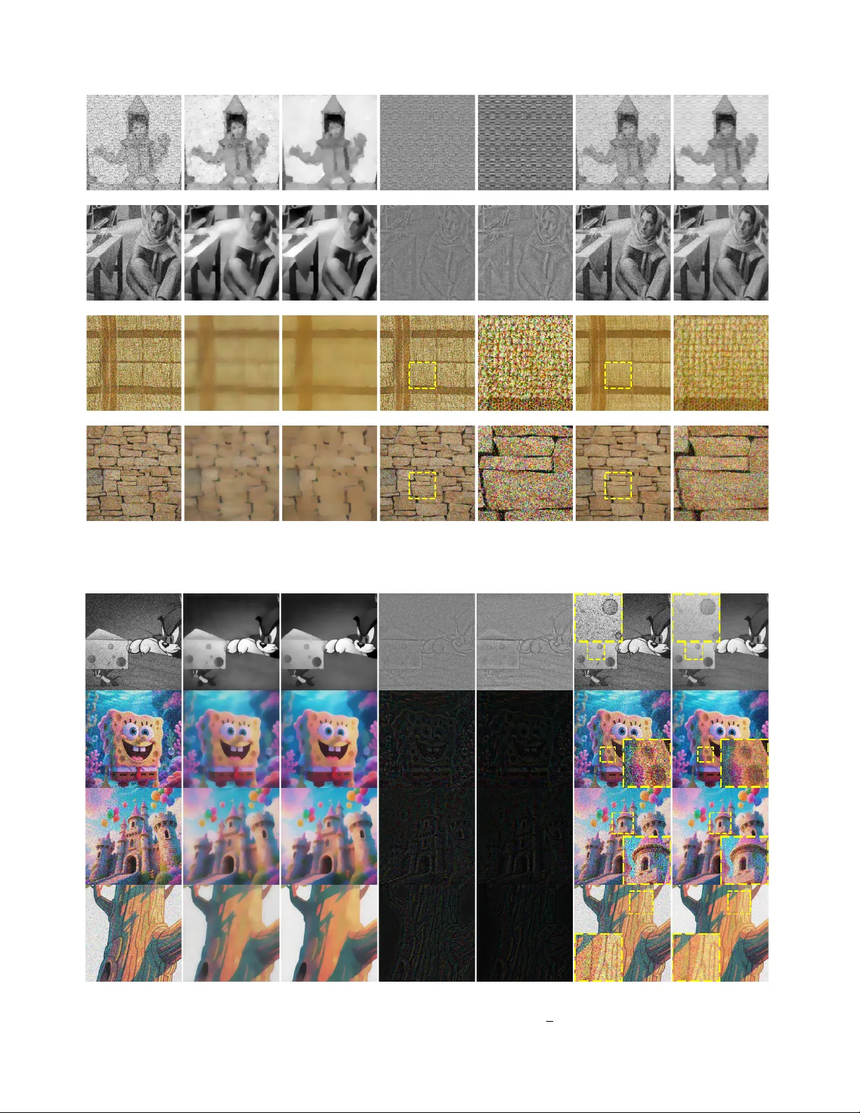
JOURNAL OF L A T E X CLASS FILES, VOL. XX, NO. XX, MARCH 2026 1 A Rob ust Lo w-Rank Prior Model for Structured Cartoon-T e xture Image Decomposition with Hea vy-T ailed Noise W eihao T ang ˙ ID and Hongjin He ˙ ID Abstract —Cartoon-texture image decomposition is a funda- mental yet challenging problem in image pr ocessing. A significant hurdle in achieving accurate decomposition is the perv asive presence of noise in the observed images, which se verely impedes rob ust results. T o address the challenging problem of cartoon- texture decomposition in the pr esence of heavy-tailed noise, we in this paper propose a robust low-rank prior model. Our approach departs from conv entional models by adopting the Huber loss function as the data-fidelity term, rather than the traditional ℓ 2 - norm, while r etaining the total variation norm and nuclear norm to characterize the cartoon and textur e components, respectiv ely . Given the inher ent structure, we employ two implementable operator splitting algorithms, tailored to different degradation operators. Extensive numerical experiments, particularly on image restoration tasks under high-intensity heavy-tailed noise, efficiently demonstrate the superior performance of our model. Index T erms —Cartoon-texture image decomposition, huber function, low-rank, heavy-tailed noise, image restoration. I . I N T RO D U C T I O N C AR T OON-TEXTURE image decomposition, which aims to split an observed image into a piece-wise smooth cartoon component that captures large-scale geometric struc- tures, and a highly-oscillatory texture component that encodes fine-scale repetitiv e patterns, is a fundamental task in modern image processing. This separation enables dedicated process- ing of each part and has proven crucial for applications such as denoising, inpainting, super-resolution, compression, and material analysis (e.g., see [ 1 ]–[ 3 ]). Mathematically , giv en an observed image b 0 ∈ R m × n , one seeks b 0 = Φ( u + v ) + ε, (1) where u denotes the cartoon part, v represents the texture component, Φ is a known linear operator (which can be the identity operator or other degradation operators, such as blurring and down-sampling operations), and ε is an unknown noise term. Generally speaking, solving the in v erse problem ( 1 ) presents significant challenges due to its underdetermined nature and sev ere ill-posedness, e v en in noise-free and pure image decom- position (i.e., Φ = I , where I represents the identity operator) scenarios. For practical applications, the key to successful decomposition from degraded measurements b 0 lies in the judicious regularization of u and v , incorporating suitable prior knowledge about their properties. As shown in [ 2 ], sparsity and compressibility assumptions often yield effecti ve Corresponding author: Hongjin He (email: hehongjin@nbu.edu.cn). The authors are with the School of Mathematics and Statistics, Ningbo Univ ersity , Ningbo 315211, China. regularizations. For this reason, we restrict our attention to structured images in which the cartoon and te xture components can be accurately characterized by widely used regularizers. In the literature, the seminal regularizer for cartoon part is the well-known T otal-V ariation (TV) semi-norm (see [ 4 ]), which is popular for its ability to preserve discontinuities (sharp edges) in images. Ho wev er , direct application of the TV model [ 4 ] lacks an explicit texture prior and tends to leav e low-frequenc y textures in the residual v . Consequently , Meyer [ 3 ] introduced the so-named dual G -norm to promote the oscillatory texture, which successfully extracts textures, yet the non-smoothness of G -norm makes the underlying optimization problem hard to solve. Subsequently , V ese and Osher [ 5 ] proposed the use of approximate dual norms and wa velet/frame-based priors, though this approach comes at the expense of either theoretical elegance or computational effi- ciency . Then, Ng et al. [ 6 ] introduced a structured optimization and an efficient multi-block splitting method to improve the quality of the decomposition. In reality , many natural images, such as facades, fabrics, or wallpapers, exhibit regular patterns that can be modeled as ap- proximately low-rank matrices. Then, Schaeffer and Osher [ 7 ] judiciously translated this observation into the Low-P atch- Rank (LPR) prior and established the following decomposition model for ( 1 ): min u,v τ ∥|∇ u |∥ 1 + µ ∥P v ∥ ∗ + 1 2 ∥ Φ( u + v ) − b 0 ∥ 2 , (2) where ∇ denotes the first-order deriv ativ e operator, P extracts ov erlapping patches and ∥ · ∥ ∗ denotes the nuclear norm. In many cases, the LPR model ( 2 ) is effecti ve when the texture is coherent across the whole image, but becomes sub-optimal for images with multiple, locally different patterns. Therefore, Ono et al. [ 8 ] proposed the Block Nuclear-Norm (BNN) prior that imposes lo w-rank constraints on local blocks instead of global patches. While BNN improv es decomposition quality , its block-wise structure increases algorithmic complexity and, more importantly , prev ents a straightforward extension to color images. Recently , Zhang and He [ 9 ] introduced the Customized Low-Rank Prior (CLRP) model for some globally well-patterned images: min u,v τ ∥|∇ u |∥ 1 + µ ∥ v ∥ ∗ + 1 2 ∥ Φ( u + v ) − b 0 ∥ 2 , (3) which directly regularizes the entire texture component by the global nuclear norm and couples it with the classical TV cartoon prior . As demonstrated in [ 9 ], the CLRP model ( 3 ) is strikingly simple, parameter-ef ficient, and naturally extends to JOURNAL OF L A T E X CLASS FILES, VOL. XX, NO. XX, MARCH 2026 2 A dd H eavy - T ai l ed N oi se CLRP M od e l RLRP M od e l S NR : 13.29 d B S NR: 19.06 d B S NR: 23.52 d B SVD SVD SVD R eco v er ed R eco v er ed C artoon : 𝒖 T e xtur e : 𝒗 Origin al Im age : 𝒃 O bser ved: 𝒃 𝟎 = 𝒃 + 𝜺 𝐦 𝐢𝐧 𝒖 , 𝒗 𝝉 | | 𝛁 𝒖 | | 𝟏 + 𝝁 | | 𝒗 | | ∗ + 𝟏 𝟐 | | 𝜱 𝒖 + 𝒗 − 𝒃 𝟎 | | 𝟐 𝐦 𝐢𝐧 𝒖 , 𝒗 𝝉 | | 𝛁 𝒖 | | 𝟏 + 𝝁 | | 𝒗 | | ∗ + 𝝆 𝒄 𝜱 𝒖 + 𝒗 − 𝒃 𝟎 T e xtur e : 𝒗 C ar toon : 𝒖 Fig. 1. A comparison between the CLRP model ( 3 ) and our RLRP model ( 10 ), which provides a conceptual explanation of the robustness of our RLRP model to heavy-tailed noise. multi-channel images. The most recent work [ 11 ] leverages iterativ e weighted least square and low-rank regularization to separately model cartoon and texture components. This approach is able to effecti vely enhance edges and suppress texture through iterative updates of an edge-preserving weight matrix. In recent years, deep learning-based image decom- position models have become a research hotspot. W ith the nonlinear fitting ability of neural networks, these models learn decomposition mapping via end-to-end training, breaking the limitation of manual regularization in traditional models. A typical work is the PnP-based decomposition method [ 12 ], which replaces regularization with deep denoisers to balance flexibility and performance. CNN, GAN and other networks are also directly used for Cartoon-T exture decomposition to achiev e end-to-end output. Note that the aforementioned approaches typically perform well in scenarios in volving no noise or white Gaussian noise. Consequently , the quadratic data fidelity term deri ved from the ℓ 2 norm is commonly employed to handle such noise. Howe v er , in practice, images are often corrupted by heavy- tailed or impulsive noise ( [ 13 ]–[ 15 ]), rendering the traditional quadratic data fidelity term highly sensitiv e and unstable. As illustrated in Fig. 1 , heavy-tailed noise significantly disrupts both gradient sparsity and low-rank properties, which encour- ages us to search more robust alternatives. Inspired by the success of the Huber function in robust regression for data fitting (widely used in machine learning and regression analysis, see [ 16 ], [ 17 ]), we adopt it to formulate the data fidelity term in this paper . Promisingly , the Huber function is a piecewise function that adaptively balances the sensitivity of the ℓ 2 -norm for moderate noise and the robustness of the ℓ 1 -norm for outliers, providing enhanced resilience against div erse noise distributions. Building on this, we propose a nov el model for decomposing an observed image corrupted by heavy-tailed noise into its cartoon and texture components. Our ke y contributions are threefold: • W e introduce a Rob ust Low-Rank Prior (RLRP) model that e xplicitly addresses hea vy-tailed noise via the Hu- ber loss. It is notew orthy that the Huber function in- corporates an adaptiv e threshold, enabling a dynamic selection between the ℓ 1 -norm and ℓ 2 -norm. For pix els with noise close to zero (near the mean), it behaves like the ℓ 2 -norm, preserving sensitivity to small deviations. For pixels heavily corrupted by outliers, where values deviate significantly from local regions, it switches to the ℓ 1 -norm, aligning with low-rank and smoothness priors. Thus, rather than enforcing strict data fidelity , our model prioritizes regularization-dri ven estimation. • W e develop globally conv ergent and efficient optimiza- tion algorithms for both identity Φ = I and general linear degradation operators Φ  = I . Due to the piece- wise structure of the Huber function, the appearance of general operator Φ makes our RLRP model more difficult than traditional models. Therefore, we introduce two cus- tomized algorithms so that they are easily implementable with closed-form solutions. Specifically , we employ the partially parallel splitting algorithm [ 18 ] with closed-form proximal updates to deal with the case Φ = I . For general operators Φ  = I , we derive a primal-dual hybrid gradient algorithm [ 19 ] with parallel and explicit updates, ov ercoming the challenges posed by the piecewise Huber loss in numerical optimization. • Through extensiv e experiments on synthetic and real- JOURNAL OF L A T E X CLASS FILES, VOL. XX, NO. XX, MARCH 2026 3 world images, we demonstrate that our RLRP model sig- nificantly outperforms traditional Gaussian-noise-based models when images are corrupted by heavy-tailed noise. This paper is organized as follows. In Section II , we first introduce the notations that will be used throughout the paper . In Section III , we propose a nov el robust low-rank prior model for ( 1 ). Then, we present two implementable algorithms for our model. In Section IV , we conduct the numerical performance of our approach (i.e., model and algorithms) on handling the heavy-tailed noise. Finally , we complete this paper with some concluding remarks in Section V . I I . N O T A T I O N S In this section, we recall some notations that will be used in this paper . Let R n represent an n -dimensional Euclidean space. For a giv en x ∈ R n , we denote ∥ x ∥ p as the ℓ p norm, i.e., ∥ x ∥ p := ( P n i =1 | x i | p ) 1 p for 1 ≤ p < ∞ , where x i is the i th component of vector x . In particular , we will use ∥ · ∥ to denote the standard ℓ 2 -norm for notational simplicity . When p = ∞ , it represents the infinity-norm defined by ∥ x ∥ ∞ := max i | x i | . Giv en a matrix X ∈ R m × n , we denote its nuclear norm by ∥ X ∥ ∗ := P r i =1 σ i ( X ) , where σ i ( X ) is the i th largest singular value of X and r := min( m, n ) . In addition, the Frobenius norm of X is defined by ∥ X ∥ F := q P m i =1 P n j =1 X 2 ij . Note that the Frobenius norm can be regarded as the ℓ 2 - norm of vector that is stacked by a matrix, so the ∥ · ∥ throughout represents the ℓ 2 -norm of a vector or the Frobenius norm of a matrix for notational simplicity . The first-order deriv ati ve operator is denoted as ∇ :=  ∇ x ∇ y  . Then, in our experiments, we will use the isotropic TV defined by ( |∇ u | ) i := p ( ∇ x u ) 2 i + ( ∇ y u ) 2 i (see [ 4 ]). Throughout this paper , I and 0 represent the identity matrix (or operator) and zero vector for simplicity . Below , we recall the proximity operator that will be used in our algorithmic implementations. For a giv en function f : R n → R ∪ { + ∞} , dom f represents its domain, and its conju- gate function is defined by f ∗ ( y ) := sup x ∈ dom f ( y ⊤ x − f ( x )) . Then, we define prox β f ( a ) := arg min x ∈ dom f  f ( x ) + 1 2 β ∥ x − a ∥ 2  (4) as the proximity operator of f , where β > 0 . Consequently , when f is specified as the indicator function associated with the set consisting of elements with bounded infinity-norm B ∞ τ = { x : max i | x i | < τ } with a gi ven τ > 0 , then the proximity operator ( 4 ) corresponds to the projection operator as follo ws: Clip τ ( a ) := sign( a ) · min( | a | , τ ) , for a ∈ B ∞ τ , (5) where ‘sign( · )’ is the sign function. Moreover , when f is taken as f ( x ) = ∥ x ∥ 1 , the proximity operator ( 4 ) reduces to the well-known shrinkage operator “shrink( · , · )” defined by shrink( a , τ ) := sign( a ) · max {| a | − τ , 0 } , (6) The shrinkage operator is also av ailable for matrices. Giv en a matrix X and a scalar τ > 0 , let X = U Σ V ⊤ be the sin- gular value decomposition (SVD) of X , the soft-thresholding operator (see [ 20 ]) S : R m × n → R m × n is defined as S ( X , τ ) = U shrink(Σ , τ ) V ⊤ . (7) T o end this section, we recall the Huber function ρ c ( x ) , which is defined as: ρ c ( x ) =  1 2 x 2 , if | x | ≤ c, c | x | − c 2 2 , if | x | > c, (8) where x ∈ R and c > 0 is a hyperparameter that determines the threshold for switching between squared and absolute loss. Interestingly , we can apply the Huber function element-wise to the entries of the matrix X ∈ R m × n and then aggregates the results, i.e., ρ c ( X ) = P m i =1 P n j =1 ρ c ( X ij ) . Note that such a function still enjoys the smoothness at x = 0 , which will be helpful in optimization. Besides, the conjugate function of the Huber function is defined as: ρ ∗ c ( x ) =  1 2 x 2 , if | x | ≤ c, + ∞ , if | x | > c. (9) I I I . T H E R L R P M O D E L A N D A L G O R I T H M S In this section, we first introduce a novel Robust Low- Rank Prior (RLRP) model for image decomposition. Then, we reformulate our proposed RLRP model as some structured optimization problems so that we can easily employ efficient optimization algorithms to obtain ideal solutions of ( 1 ). A. The RLRP model As demonstrated in [ 9 ], texture components can be ef- fectiv ely characterized by a low-rank function when images contain large and well-preserved texture regions. A widely used con v ex surrogate for low-rank functions is the nuclear norm, which has prov en highly successful in image and video processing. Meanwhile, the TV norm is an ideal choice for regularizing the cartoon component due to its ability to cap- ture the smooth continuity of the background. Following the approach of [ 9 ], we therefore adopt the TV norm and nuclear norm to regularize the cartoon and texture parts, respectively . In the literature, the standard ℓ 2 -norm has been sho wn to effecti v ely handle Gaussian noise. Howe ver , for heavy-tailed noise (e.g., t-distrib uted noise), the quadratic growth of the ℓ 2 -norm often leads to suboptimal performance. Consequently , the traditional ℓ 2 -norm is not ideal for heavy-tailed noise (see Fig. 1 ), as further e videnced by our numerical experiments (Section IV ). T o address this, we replace the ℓ 2 -norm with the Huber function for the data fidelity term. Specifically , our Robust Low-Rank Prior (RLRP) model is formulated as: min u,v τ ∥|∇ u |∥ 1 + µ ∥ v ∥ ∗ + ρ c (Φ( u + v ) − b 0 ) , (10) where ρ c ( · ) is defined by ( 8 ), τ and µ are positiv e regulariza- tion parameters balancing the contributions of the cartoon and texture components. It is easy to see from ( 10 ) that the piece-wise structure of the Huber function and the coupling of u and v through the degraded operator Φ make directly solving ( 10 ) nontrivial. Be- sides, when Φ = I or B being the blurring operator , the related JOURNAL OF L A T E X CLASS FILES, VOL. XX, NO. XX, MARCH 2026 4 subproblems usually can be solved with lo w computational cost after a F ast F ourier T ransformation (FFT). Ho wev er , when Φ = S being the down-sampling operator , which cannot be transferred into a diagonal form, thereby making the related subproblems more dif ficult. Thus, ef fectiv ely exploiting the structure of ( 10 ) is essential for de vising an ef ficient algorithm. T o address this, we below dev elop two tailored algorithms for the cases Φ = I and Φ  = I , respectively . B. Solving model ( 10 ) with Φ = I Note that the objectiv e function of ( 10 ) is the sum of three con ve x functions, and each of them has their own structure. Moreov er , the last Huber loss function has coupled variables u and v . Therefore, we introduce two auxiliary variables y and z to fully separate the three objectives. Specifically , we let ∇ u = y and Φ( u + v ) = z with Φ = I , then ( 10 ) can be recast as min µ ∥ v ∥ ∗ + τ ∥| y |∥ 1 + ρ c ( z − b 0 ) s.t.  ∇ I  u +  O I  v +  − I O O − I   y z  = 0 , (11) where O represents the zero matrix. Consequently , by letting A =  ∇ I  , B =  O I  , C =  − I O O − I  , w =  y z  , the model ( 11 ) falls into a standard linearly constrained three- block separable conv ex minimization problem: min u,v ,w f ( u ) + g ( v ) + h ( w ) s . t . Au + B v + C w = 0 , (12) where      f ( u ) = 0 , g ( v ) = µ ∥ v ∥ ∗ , h ( w ) = τ ∥| y |∥ 1 + ρ c ( z − b 0 ) . Now , we first construct the augmented Lagrangian function: L β ( u, v , w, λ ) = f ( u ) + g ( v ) + h ( w ) − λ ⊤ ( Au + B v + C w ) + β 2 ∥ Au + B v + C w ∥ 2 , (13) where β > 0 is a penalty parameter , and λ is called Lagrangian multiplier associated to the linear constraints in ( 12 ). Then, by the algorithmic frame work introduced in [ 18 ], we follow the order u → λ → v → w to make a prediction step. Specifically , we sho w their explicit iterativ e schemes as follo ws. • Update u k +1 via u k +1 = arg min u  f ( u ) + β 2 s ∥ Au + a k u ∥ 2  = arg min u β 2 s (     ∇ u − y k − s β λ k 1     2 +     u + v k − z k − s β λ k 2     2 ) . where a k u = B v k + C w k − s β λ k . As a consequence, by the first-order optimality condition, we easily obtain ( ∇ ⊤ ∇ + I ) u k +1 = ∇ ⊤  y k + s β λ k 1  +  z k − v k + s β λ k 2  . (14) • Compute a prediction ˜ λ k via ˜ λ k = λ k − β s  Au k +1 + B v k + C w k  . (15) By the block structure of A, B , C , we let λ = ( λ ⊤ 1 , λ ⊤ 2 ) ⊤ , then ( 15 ) can be rewritten as  ˜ λ k 1 ˜ λ k 2  =  λ k 1 − β s  ∇ u k +1 − y k  λ k 1 − β s  u k +1 + v k +1 − z k   . (16) • Generate ˜ v k and ˜ w k simultaneously via    ˜ v k = arg min v n g ( v ) + rβ 2 ∥ B v − a k v ∥ 2 o , ˜ w k = arg min w n h ( w ) + rβ 2 ∥ C w − a k w ∥ 2 o , (17) where        a k v = v k + 1 rβ (2 ˜ λ k 2 − λ k 2 ) , a k w = a k y a k z ! =   − y k + 1 rβ  2 ˜ λ k 1 − λ k 1  − z k + 1 rβ  2 ˜ λ k 2 − λ k 2    . By inv oking the fact g ( v ) = µ ∥ v ∥ ∗ , the prediction on ˜ v k in ( 17 ) is specified as ˜ v k = arg min v  µ ∥ v ∥ ∗ + r β 2 ∥ v − a k v ∥ 2  = S  a k v , µ r β  . (18) where S ( · , · ) is giv en in ( 7 ). W ith the notation h ( w ) , the prediction on ˜ w k in ( 17 ) reads as ˜ w k = arg min w τ ∥| y |∥ 1 + ρ c ( z − b 0 ) + r β 2      y + a k y z + a k z      2 . By the separability of the h ( w ) with respect to y and z , the abov e subproblem is separated into two subproblems on y and z . So, we can also update ˜ y k and ˜ z k in a parallel way . – First, the prediction ˜ y k reads as ˜ y k = arg min y  τ ∥| y |∥ 1 + r β 2 ∥ y + a k y ∥ 2  =shrink  − a k y , τ r β  . (19) where shrink( · , · ) is defined by ( 6 ). – Similarly , the prediction ˜ z k arriv es at ˜ z k = arg min z  ρ c ( z − b 0 ) + r β 2 ∥ z + a k z ∥ 2  = pro x 1 rβ ρ c ( · ) ( − b 0 − a k z ) + b 0 , (20) where the proximity operator of Huber function is JOURNAL OF L A T E X CLASS FILES, VOL. XX, NO. XX, MARCH 2026 5 defined as prox β ρ c ( · ) ( x ) = ( prox β 2 ∥·∥ ( x ) , if | x | ≤ c prox cβ ∥·∥ 1 ( x ) , if | x | > c. • Finally , we make a correction on ( v k +1 , w k +1 , λ k +1 ) via a relaxation step: ζ k +1 =   v k +1 w k +1 λ k +1   =   v k w k λ k   − γ   v k − ˜ v k w k − ˜ w k λ k − ˜ λ k   . (21) W ith the above deriv ations of all subproblems, we can sum- marize them into Algorithm 1 . Algorithm 1 Solving problem ( 10 ) when Φ = I . Require: Set initial points ( v 0 , y 0 , z 0 , λ 0 1 , λ 0 2 ) , penalty param- eter β > 0 , γ ∈ (0 , 2) , r and s satisfying r s > 2 , and a tolerance ϵ > 0 . 1: for k = 0 , 1 , · · · do 2: Update u k +1 via ( 14 ). 3: Compute ˜ λ k 1 and ˜ λ k 2 via ( 16 ). 4: Predict ˜ v k via ( 18 ). 5: Generate ˜ y k and ˜ z k via ( 19 ) and ( 20 ), respectively . 6: Correct ( v k +1 , w k +1 , λ k +1 ) via ( 21 ). 7: end for Note that ( 10 ) is equiv alent to the following saddle point problem: max λ min u,v ,w L 0 ( u, v , w, λ ) , (22) where L 0 is giv en by ( 13 ) with setting β = 0 . Consequently , by letting Q =   r β B ⊤ B O − B ⊤ O r β C ⊤ C − C ⊤ − B − C s β I   , it follows from [ 18 , Theorem 3.2] that Algorithm 1 is globally con ver gent and has the worst-case O (1 / N ) con ver gence rate under the condition r s > 2 (which ensures the positiv e definiteness of Q ). Here, we skip its proof for the conciseness of this paper . The readers who are concerned with its details can refer to [ 18 ]. Theorem 1. Let Ω ∗ be the solution set of ( 22 ) and ∆ ∗ := { ζ ∗ = ( v ∗ , w ∗ , λ ∗ ) | ξ ∗ ∈ Ω ∗ } , wher e ξ ∗ = ( u ∗ , v ∗ , w ∗ , λ ∗ ) . Then, the sequences { ξ k } , { ζ k } , and { ¯ ζ k } gener ated by Algorithm 1 satisfy the following assertions: (a). The sequence of subvectors { ζ k } of { ξ k } con ver ges globally to a member of ∆ ∗ . (b). F or any integ er number N > 0 , we have    ζ N − ˜ ζ N    2 Q ≤ 1 γ (2 − γ )( N + 1)   ζ 0 − ζ ∗   2 Q , wher e the Q-norm of x ∈ R n is defined by ∥ x ∥ Q := p x ⊤ Qx . C. Solving model ( 10 ) with Φ  = I As discussed in Section III-B , when Φ differs from the identity operator , the u -subproblem no longer retains the simplicity of ( 14 ). Moreover , the v -subproblem will lose its explicit form of the proximity operator . In this case, the aforementioned partially parallel splitting method [ 18 ] is not necessarily the best choice for Φ  = I . Therefore, we first reformulate ( 10 ) as a structured conv ex-conca ve saddle point problem, which is beneficial for employing the popular first- order primal-dual algorithm [ 19 ] to solve the problem under consideration. First, by letting ∇ u = x and Φ( u + v ) = z , we can rewrite ( 10 ) as min u,v ,x,z τ ∥| x |∥ 1 + µ ∥ v ∥ ∗ + ρ c ( z − b 0 ) s.t.  ∇ Φ  u +  O Φ  v −  x z  = 0 . (23) Consequently , its Lagrangian function reads as: L ( u, v , x, z , λ 1 , λ 2 ) = τ ∥| x |∥ 1 + µ ∥ v ∥ ∗ + ρ c ( z − b 0 ) + ⟨ λ 1 , ∇ u − x ⟩ + ⟨ λ 2 , Φ( u + v ) − z ⟩ . Clearly , due to conv exity of ( 23 ), it easily follows from [ 21 , Section 5.3.2] that solving ( 23 ) is equi v alent to finding a saddle point of the following problem: min ( u,v ,x,z ) max ( λ 1 ,λ 2 ) L ( u, v , x, z , λ 1 , λ 2 ) . (24) T o further simplify ( 24 ) and reformulate it as a structured saddle point problem, by using the notation x = ( u ⊤ , v ⊤ ) ⊤ , y = ( x ⊤ , z ⊤ ) ⊤ , λ = ( λ ⊤ 1 , λ ⊤ 2 ) ⊤ , it follo ws from the definition of conjugate function and ( 9 ) that min y L ( y , λ ) = min x,z τ ∥| x |∥ 1 + ρ c ( z − b 0 ) − ⟨ λ 1 , x ⟩ − ⟨ λ 2 , z ⟩ = sup x,z ⟨ λ 1 , x ⟩ + ⟨ λ 2 , z ⟩ − τ ∥| x |∥ 1 − ρ c ( z − b 0 ) = sup x {⟨ λ 1 , x ⟩ − τ ∥| x |∥ 1 } + sup z {⟨ λ 2 , z ⟩ − ρ c ( z − b 0 ) } = ( τ ∥| x |∥ 1 ) ∗ ( λ 1 ) + ( ρ c ( z − b 0 )) ∗ ( λ 2 ) = δ ∥ λ 1 ∥ ∞ ≤ τ + ρ ∗ c ( λ 2 ) + ⟨ λ 2 , b 0 ⟩ = F ∗ ( λ 1 , λ 2 ) , which immediately implies that ( 24 ) can be recast as min u,v max λ 1 ,λ 2 ⟨∇ u, λ 1 ⟩ + ⟨ Φ( u + v ) , λ 2 ⟩ | {z } ⟨ K x , λ ⟩ + µ ∥ v ∥ ∗ | {z } G ( x ) −  δ ∥ λ 1 ∥ ∞ ≤ τ + ρ ∗ c ( λ 2 ) + ⟨ λ 2 , b 0 ⟩  | {z } F ∗ ( λ ) ≡ F ∗ ( λ 1 ,λ 2 ) , where K x =  ∇ u Φ( u + v )  =  ∇ O Φ Φ   u v  . Therefore, by the employment of the first-order primal-dual algorithm [ 19 ] for min x max λ ⟨ K x , λ ⟩ + G ( x ) − F ∗ ( λ ) , (25) JOURNAL OF L A T E X CLASS FILES, VOL. XX, NO. XX, MARCH 2026 6 the iterati ve scheme is specified as      λ k +1 = prox σ F ∗ ( λ k + σ K ¯ x k ) , x k +1 = prox η G ( x k − η K ⊤ λ k +1 ) , ¯ x k +1 = 2 x k +1 − x k . (26) More concretely , for giv en the k -th iteration, λ k 1 , λ k 2 , u k , v k , ¯ u k , and ¯ v k , the iterative scheme ( 26 ) is specified as • Update dual variables λ k +1 1 and λ k +1 2 via: λ k +1 1 = prox σ δ ∥ λ 1 ∥ ∞ ≤ τ ( λ k 1 + σ ∇ ¯ u k ) = Clip τ ( λ k 1 + σ ∇ ¯ u k ) , (27) λ k +1 2 = prox σ ( ρ ∗ c ( λ 2 )+ ⟨ λ 2 ,b 0 ⟩ ) ( λ k 2 + σ Φ( ¯ u k + ¯ v k )) = prox σ ρ ∗ c ( · ) ( λ k 2 + σ Φ( ¯ u k + ¯ v k ) − σ b 0 ) , (28) where the proximity operator of the Huber function’ s conjugate function is defined as: prox σ ρ ∗ c ( x ) =  x 1+ σ , if | x | ≤ ( σ + 1) c, c · sign ( x ) , if | x | > ( σ + 1) c. • Update primal variables u k +1 and v k +1 via: u k +1 = u k − η  ∇ ⊤ λ k +1 1 + Φ ⊤ λ k +1 2  , (29) v k +1 = prox η µ ∥·∥ ∗ ( v k − η Φ ⊤ λ k +1 2 ) = S  v k − η Φ ⊤ λ k +1 2 , η µ  . (30) • Do the extrapolation step: ¯ u k +1 = 2 u k +1 − u k , (31) ¯ v k +1 = 2 v k +1 − v k . (32) W ith the abov e preparations, we can summarize them in Algorithm 2 . Algorithm 2 Solving problem ( 23 ) with Φ  = I . Require: Set initial points ( u 0 , v 0 , λ 0 1 , λ 0 2 , ¯ u 0 , ¯ v 0 ) , and σ > 0 , η > 0 satisfying √ σ η < 1 ∥ K ∥ . 1: for k = 0 , 1 , · · · do 2: Update λ k +1 1 and λ k +1 1 via ( 27 ) and ( 27 ), respectiv ely . 3: Update u k +1 and v k +1 via ( 29 ) and ( 29 ), respectively . 4: Compute ¯ u k +1 and ¯ v k +1 via ( 31 ) and ( 32 ), respectiv ely . 5: end for Under the condition √ σ η < 1 ∥ K ∥ , it follows from [ 19 , Theorem 1] that Algorithm 2 also enjoys a global conv ergence and the O (1 / N ) conv ergence rate. The complete proof is referred to [ 19 ] for the conciseness of this paper . Theorem 2. Let ( ˆ x , ˆ λ ) be a saddle point of ( 25 ) and { ( x k , λ k , ¯ x k ) } be the sequence gener ated by ( 26 ) (i.e., Al- gorithm 2 ). Then: (a). Ther e exists a saddle-point ( x ⋆ , λ ⋆ ) such that x k → x ⋆ and λ k → λ ⋆ . (b). F or any k , { ( x k , λ k ) } r emains bounded and satisfies ∥ λ k − ˆ λ ∥ 2 2 σ + ∥ x k − ˆ x ∥ 2 2 η ≤ C ∥ λ 0 − ˆ λ ∥ 2 2 σ + ∥ x 0 − ˆ x ∥ 2 2 η ! , wher e the constant C ≤ (1 − ησ ∥ K ∥ 2 ) − 1 . (c). Let x N = ( P N k =1 x k ) / N and λ N = ( P N k =1 λ k ) / N , for any bounded set B 1 × B 2 , the r estricted primal-dual gap has the following bound: G B 1 × B 2 ( x N , λ N ) ≤ D ( B 1 , B 2 ) N , (33) wher e G B 1 × B 2 ( x , λ ) = max λ ′ ∈ B 2 {⟨ λ ′ , K x ⟩ − F ∗ ( λ ′ ) + G ( x ) } − min x ′ ∈ B 1 {⟨ λ , K x ′ ⟩ − F ∗ ( λ ) + G ( x ′ ) } , r epr esents the primal-dual gap and D ( B 1 , B 2 ) = sup ( x , λ ) ∈ B 1 × B 2  ∥ x − x 0 ∥ 2 2 η + ∥ λ − λ 0 ∥ 2 2 σ  . Mor eover , the weak cluster points of ( x N , λ N ) are saddle-points of ( 25 ) . I V . E X P E R I M E N TA L R E S U LT S In this section, we conduct the performance of our RLRP model ( 10 ) on some image processing problems. W e consider three scenarios in our experiments: (i). Φ = I , which corre- sponds to the pure image denoising of an observ ation with heavy-tailed noise. (ii). Φ = S , which represents a down- sampling operator including the binary “mask” and random sampling. (iii). Φ = B , which is a blurring operator . T o verify the robustness of our model to heavy-tailed noise, for all the abov e cases, we will compare our approach (denoted by RLRP ) with the G-norm model [ 6 ] ( NYZ in short), the LPR model [ 22 ] ( HKZ in short), the BNN model [ 8 ] ( OMY in short), and the customized LRP model [ 9 ] ( CLRP in short). In addition, there are recent models such as the L 0 gradient model [ 10 ] ( PWH in short), the WLS model [ 11 ] ( L WC in short), and the PnP network model [ 12 ] ( GA T in short). W e set the initial points as u 0 = ¯ u 0 = b 0 , and other variable are taken as zero matrices (or vectors). Besides, the stopping criterion is taken as follows for all experiments: T ol = max  ∥ u k +1 − u k ∥ ∥ u k ∥ + 1 , ∥ v k +1 − v k ∥ ∥ v k ∥ + 1  < ϵ, (34) where the tolerance ϵ is a positive constant, which was set the same v alue of ϵ in the same experiment. All test images are displayed in Fig. 2 . Among the selected images, there are grayscale images (a), (b) and RGB color images (c)-(j). Image (a) is a synthetic image, formed by su- perimposing the cartoon component and the te xture component in a 7:3 ratio. Images (b)-(f) are real-world images and have relativ ely distinct and well-preserved texture patterns. Images (g)-(j) are colored piece-wise continuous and smooth cartoon- like images with distinct locally clear textures. And all tested images are scaled into [0 , 1] . All numerical e xperiments are implemented in P Y T H O N 3.11 and are conducted on a laptop computer with Intel(R) Core(TM) i5 CPU 2.61GHz and 16G memory . JOURNAL OF L A T E X CLASS FILES, VOL. XX, NO. XX, MARCH 2026 7 (a) (b) (c) (d) (e) (f ) (g) (h) (i) (j) Fig. 2. T est images. (a) Boy synthetic image ( 256 × 256 ); (b) Barbara natural image ( 512 × 512 ); (c) Stone natural image ( 512 × 512 × 3 ); (d) T owel natural image ( 512 × 512 × 3 ); (e) Kodim wall natural image ( 512 × 512 × 3 ); (f) Barbar a RGB natural image ( 512 × 512 × 3 ); (g) T omJerr y cartoon image ( 512 × 512 ); (h) Sponge Bob cartoon image ( 512 × 512 × 3 ); (i) Castle cartoon image ( 512 × 512 × 3 ); (j) Bole cartoon image ( 512 × 512 × 3) . A. Pur e image denoising In this subsection, we consider the pure image denoising of observed images corrupted by heavy-tailed noise. W e select 8 images and divided into 2 groups. These images are used to test the restoration ability of the model for grayscale im- ages, RGB color images, synthetic images, real-world images, cartoon-like images and images with good patterns respec- tiv ely . Regarding the parameter settings, for the synthetic image (a), we set τ = 0 . 1 and µ = 2 for model ( 10 ). For the rest of images, we set τ = 0 . 015 and µ = 0 . 2 . For these algorithmic parameters, as described in [ 9 ] for ( 3 ), we set γ = 1 . 3 for image (a), while for other images, we set γ = 1 . 6 , and r = 1 , s = 2 . 01 for all. The student’ s-t distrib ution is a typical symmetric hea vy-tailed distribution. As the degrees of freedom increase, it increasingly approaches the Gaussian distribution. When the degrees of freedom is 2 , its heavy-tailed effect is the most pronounced (see [ 23 ]). For gray images (a), (b), (g), we added standard Student’ s-t noise with intensity of 0 . 1 and 0 . 2 for rest. The degrees of freedom are both 2 . For the synthetic image (a), we set the threshold parameter c = 0 . 1 of the Huber function, the algorithmic parameter β = 2 , and the stopping value ϵ = 10 − 2 giv en in ( 34 ). For the other images, we set β = 0 . 2 , ϵ = 10 − 2 and the threshold c = 0 . 01 . The signal- to-noise ratio (SNR), which is typically used to ev aluate the quality of the image, is defined by SNR = 20 log 10 ∥ b ∥ ∥ ˜ b − b ∥ , where b is the original image, ˜ b is the restored image. Another popular metric used to ev aluate image quality is the structural similarity (SSIM, see details in [ 24 ]). Based on the numerical results, the performance levels of the existing models are comparatively similar . T o enhance clarity and conciseness, rather than enumerating the results of ev ery model for all images individually , we hav e chosen the CLRP model as a representativ e benchmark. Its comparativ e performance against the RLRP model is illustrated in Fig. 3 and Fig. 4 . The complete set of numerical results is provided in T able I . As illustrated in Fig. 3 , the CLRP model struggles to iden- tify outliers under significant heavy-tailed noise interference. Consequently , the cartoon component is heavily corrupted by outliers. This is particularly evident in the synthetic image, where numerous noise points remain unsmoothed. Addition- ally , the texture component is also adversely affected, leading to the misclassification of certain cartoon patterns as texture. For natural images, CLRP and RLRP exhibit broadly similar performance due to their analogous algorithmic structures. Howe ver , in the restoration results of cartoon-like images in Fig. 4 , RLRP shows better textures and less noise. W e attribute this difference to the disruptiv e effects of high- intensity heavy-tailed noise, which compromises the inherent low-rank properties of certain patterns. Compared with CLRP , the adaptiv e thresholding mechanism of RLRP can ef fectiv ely identify outliers and utilize prior information to restore latent textures. T o further ev aluate noise resilience across models, we compared the restoration performance of different models. The experimental results show that, apart from RLRP which can achiev e excellent denoising results, the performance of other models is similar to that of CLRP , lacking a mechanism for outlier detection. Figure 5 presents the restoration results of image (a) obtained by all comparative models, including the restored images and the reconstructed texture component v . Experimental results show that the overall smoothness of the image restored by the RLRP model is significantly better than that of other models, with no obvious noise remaining, and the extracted texture component is fine and realistic. Other models suffer from strong noise interference, losing accurate texture discrimination ability; their extracted texture components are cov ered or even completely corrupted by noise. These results verify that the proposed model has excellent resistance to heavy-tailed noise. JOURNAL OF L A T E X CLASS FILES, VOL. XX, NO. XX, MARCH 2026 8 Image with Noise CLRP: u RLRP: u CLRP: v RLRP: v CLRP: u + v RLRP: u + v CLRP: u + v RLRP: u + v RLRP: u + v CLRP: u + v Fig. 3. Results for clear image decomposition: Φ = I . From left to right: the noisy image, comparison of the cartoon part, comparison of the texture part, comparison of the restored images (left: CLRP , right: RLRP). From top to bottom: Boy , Barbara , T owel and Stone respectively . Image with Noise CLRP: u RLRP: u CLRP: v RLRP: v CLRP: u + v RLRP: u + v Fig. 4. Results for cartoon image decomposition: Φ = I . From left to right: the noisy image, comparison of the cartoon part, comparison of the te xture part, comparison of the restored images (left: CLRP , right: RLRP). From top to bottom: T omJerr y , Sponge Bob , Castle and Bole respectively . JOURNAL OF L A T E X CLASS FILES, VOL. XX, NO. XX, MARCH 2026 9 NYZ : u + v NYZ : v HKZ : u + v HKZ : v OMY : u + v OMY : v CLRP : u + v CLRP : v RLRP : u + v RLRP : v L WC : u + v L WC : v PWH : u + v PWH : v GA T : u + v GA T : v Fig. 5. The decomposition results of Boy under different models (left: u + v , right: v .) Furthermore, we conduct a comprehensi ve ev aluation of noise robustness by comparing the proposed model with ex- isting approaches across varying noise intensities. As demon- strated in Fig. 6 , our model consistently outperforms the other methods, maintaining superior performance under both mild and sev ere noise conditions. This robust performance advantage is particularly e vident in the signal-to-noise ratio analysis. T o rigorously v alidate the robustness of our proposed model, we conducted extensi ve experiments with multiple heavy- tailed noise distributions beyond the t-distribution, including the Cauchy distribution and Generalized Error Distribution (GED). The Cauchy distribution represents an extreme case of heavy-tailed behavior . Unlike distributions with finite mo- ments, it lacks well-defined mean and variance, with its tail decaying at a rate of x − 2 . This characteristic leads to frequent extreme outliers, making it significantly heavier -tailed than JOURNAL OF L A T E X CLASS FILES, VOL. XX, NO. XX, MARCH 2026 10 0.04 0.06 0.08 0.1 0.12 0.14 0.16 0.18 0.2 Noise In tensity 8 10 12 14 16 18 20 22 24 26 SNR(dB) RLRP CLRP NYZ HKZ OMY 0.04 0.06 0.08 0.1 0.12 0.14 0.16 0.18 0.2 Noise In tensity 5 10 15 20 SNR(dB) RLRP CLRP NYZ HKZ OMY Fig. 6. The SNR values of dif ferent noise intensity . Left: Boy , right: Barbara . Boy t Cauchy Ged 0 5 10 15 20 25 SNR CLRP NYZ HKZ OMY RLRP Barbara t Cauchy Ged 0 5 10 15 SNR CLRP NYZ HKZ OMY RLRP Bob t Cauchy Ged 0 2 4 6 8 10 12 14 SNR CLRP NYZ HKZ RLRP Bole t Cauchy Ged 0 5 10 15 SNR CLRP NYZ HKZ RLRP Fig. 7. The SNR values of images restored by dif ferent models under different types of noise, in the order of Boy , Barbara , Sponge Bob , Bole . the t-distribution (see [ 25 ]). The GED offers more flexible tail behavior through its shape parameter . While maintaining heavy-tailed properties, its tail decay is moderately lighter than the t-distribution (see [ 26 ]). As evidenced by Fig. 7 , our RLRP model demonstrates exceptional resilience against all tested heavy-tailed noises, consistently maintaining superior SNR values compared to baseline methods. All numerical results are summarized in T able I , with the proposed approach’ s performance highlighted in bold for clarity . Our approach demonstrates consistently superior performance across nearly all test images, achieving SNR values that are 3-5 dB higher than existing methods. This significant improv ement clearly validates the approach’ s en- hanced capability in handling high-intensity noise interference. Regarding computational efficiency , while our model shares the same regularization terms with the CLRP , its more difficult data fidelity term leads to increased solution complexity . Con- sequently , the computational time is approximately doubled compared to baseline algorithms. In future, we will discuss potential optimization strategies to achieve a better trade-off between performance gains and computational ov erhead for practical applications. B. Image inpainting In this part, we are concerned the performance of our approach on image inpainting. First, for the mask do wn-sampling operator, we select three images to conduct the noise resistance ability of the model for low-rank patterns, grayscale images, and color images respectiv ely . Specifically , we add t-noise with an intensity of 0 . 05 to the original images, and then add a binary mask. Regarding the model parameters, we uniformly set τ = 0 . 015 , µ = 0 . 2 . For the algorithm of solving ( 3 ) introduced in [ 9 ], we set β = 2 , γ = 1 . 6 , r = 1 , s = 2 . 01 . For our approach, we uniformly set σ = η = 0 . 35 and 500 as the maximum number of iterations. For each image, the stopping tolerance is set to ϵ = 2 . 5 × 10 − 4 . Fig. 8 clearly demonstrates the superior performance of our RLRP compared to the original CLRP when using identical stopping criteria. Our approach exhibits sev eral notable advan- tages in texture reconstruction: (i) effecti ve noise suppression while maintaining texture fidelity , (ii) precise restoration of missing components through rigorous low-rank optimization rather than simple pixel approximation, and (iii) significantly cleaner visual outputs that highlight its enhanced noise resis- tance capabilities relative to the CLRP model. These qualitativ e observations are quantitativ ely supported by the results presented in T able II , which shows that our RLRP consistently achiev es SNR improvements of 2-3 dB across all test images compared to other approaches. The combination of superior visual quality and measurable per - formance metrics confirms the effecti veness of our approach RLRP in both te xture preservation and noise suppression tasks. Now , to ev aluate the performance of our approach under random down- sampling, we select fiv e representativ e images: (b), (e), and (h)–(j). First, we corrupt the original images with t-noise (intensity is 0 . 1 , degrees of freedom is 2 ), followed by random down-sampling at a sampling probability of 0 . 4 . Unlike mask-based de gradation, random down-sampling in- troduces more significant perturbations to the noise’ s prior distribution, particularly as the down-sampling ratio increases. For consistency , we employ identical model parameters across all test images: τ = 0 . 015 , µ = 0 . 2 , c = 0 . 02 , β = 2 , γ = 1 . 6 , r = 1 , s = 2 . 01 , σ = η = 0 . 4 , ϵ = 10 − 2 . As illustrated in Figs. 9 , under identical noise intensity and do wn-sampling conditions, our RLRP model achieves superior restoration of color images, yielding clearer textures with better structure and background separation. In contrast, the CLRP model suffers from noise contamination in the car- toon component, exhibiting noticeable outliers. These results demonstrate that our RLRP model effecti vely adapts to heavy- tailed noise distribution shifts induced by down-sampling, outperforming the CLRP approach. Quantitativ e support is provided in T able III , where the images reconstructed by our RLRP exhibit significantly higher SNR values than the other methods. Notably , for random down-sampling, the computational ef ficiency of RLRP remains competitiv e, with iteration counts and running time compara- ble to other cases, further underscoring its practical advantage. C. Image deblurring In this subsection, we further consider the noise resistance experiment in which the known blurring operator Φ = B acts on the images. W e ev aluate our model using six test images: (a), (b), (e), and (h)-(j). Each image undergoes blur- ring through a 4 × 4 average kernel. T o comprehensively assess model performance under varying noise conditions, we apply t-distributed noise with different parameters: images JOURNAL OF L A T E X CLASS FILES, VOL. XX, NO. XX, MARCH 2026 11 Masked Image with Noise CLRP: u + v RLRP: u + v Fig. 8. Results for masked images: Φ = S . From top to bottom: K odim wall , Barbara RGB . From left to right: the masked images, comparison of the restored images, comparison of the locally magnified images. (left CLRP , right RLRP). Sampled Image with Noise CLRP: u RLRP: u CLRP: u + v RLRP: u + v Fig. 9. Results for downsampled cartoon images: Φ = S . From top to bottom: Sponge Bob , Castle , Bole . From left to right: the downsampled images, comparison of the component u , comparison of restored images. (left CLRP , right RLRP). (a), (b), and (e) degraded by noise with intensity 0.01 and 2 degrees of freedom, while images (h)-(j) are corrupted with stronger noise (intensity is 0.1). The efficac y of blurred-image restoration is particularly sensitive to noise lev els [ 27 ]. This is primarily because the blurring process modifies the intrinsic noise characteristics, such as by introducing a smoothing effect. This phenomenon creates substantial challenges for the extraction of texture components from blurred images contaminated by heavy-tailed noise. Regarding the model parameters, for the synthetic image (a) and cartoon-like images (h)-(j), we set τ = 10 − 3 , µ = 0 . 1 , and natural images (b),(e), we set τ = 10 − 5 , µ = 10 − 4 . For our approach, we set c = 0 . 03 , σ = η = 0 . 6 . Regarding the algorithm of solving ( 3 ), we set γ = 1 . 6 , r = 1 , s = 2 . 01 . Our computational experiences show that penalty parameter β is important for algorithmic implementation. For different images, (a) and (e) hav e large-scale structures, (b) only has local textures, and cartoon-type images (h)-(j) have only piece-wise smooth structures. The influence of noise on the restoration of textures in these images increases gradually . Therefore, setting the penalty parameter β to 0 . 1 , 1 . 5 , and 2 respectiv ely is a reasonable way to balance the restoration difficulty , so that different algorithms can be compared on the premise of restoring high-quality images. JOURNAL OF L A T E X CLASS FILES, VOL. XX, NO. XX, MARCH 2026 12 Blur Image with Noise CLRP: v RLRP: v CLRP: u + v RLRP: u + v CLRP: v RLRP: v CLRP: u RLRP: u Fig. 10. Results for blured images: Φ = B . From top to bottom: Boy , Kodim wall . From left to right: the downsampled images, comparison of the components (top v , bottom u ), comparison of restored images. (left CLRP , right RLRP). The restoration results are comprehensiv ely presented in Figures 10 and 11 . Figure 10 shows that when processing the synthetic image (a) under the combined effects of the blurring operator B and heavy-tailed noise, the CLRP model produces significantly distorted texture components compared to the original image. This degradation primarily stems from two factors: (i) the model’ s strict adherence to low-rank constraints forces improper texture classification; (ii) noise interference disrupts the critical distinction between authentic low-rank textures and outlier components, ultimately compromising the accurate separation of cartoon and texture elements. In contrast, our RLRP model exhibits markedly superior perfor- mance. Its restored results show three ke y advantages: (i) com- plete absence of visible noise artifacts in texture regions; (ii) effecti ve resistance to the smearing effects typically induced by average blurring operations, and (iii) precise component separation that pre vents cartoon patterns from appearing in texture regions. These improvements collecti vely demonstrate the model’ s enhanced capability to handle the challenging situations of simultaneous blurring and heavy-tailed noise contamination. This phenomenon is more pronounced in the comparison of cartoon-like images presented in Fig. 11 . For the CLRP model, the recovered texture is exceedingly faint, nearly imperceptible. This is caused by the repeated appear- ance of high-intensity noise that has not been eliminated in the image after multiple blurring processes. In images with poorly defined textures, this effect may result in the signal intensity being lo wer than the noise intensity , corresponding to an SNR value less than zero (SNR < 0 ). All numerical results are summarized in T able IV . It is evident that, in the case of Φ = B , the performance of our RLRP model exhibits the most significant contrast compared to other models. Particularly for low-rank and cartoon-like images, its SNR value is 6 or even up to 10 units higher than those of competing models. The presence of the blur - ring operator further illustrates that our RLRP model has effecti vely mitigated the impact of heavy-tailed noise and accurately recovered the underlying textures. Furthermore, it can be observed that the RLRP model solved via Algorithm 2 demonstrates comparable performance in terms of iteration count and computing time with other algorithms, and in some cases, it is even faster . V . C O N C L U S I O N W e hav e developed a robust cartoon-texture decomposition model (RLRP in short) capable of handling heavy-tailed noise contamination. The proposed approach utilizes the Huber function for noise characterization and employs both split- ting algorithms to efficiently solve the model under v arious linear degradation operators. Extensiv e numerical experiments demonstrate the proposed RLRP’ s superior noise resistance capabilities across different degradation scenarios, particularly outperforming existing methods in processing images with piecewise continuous smoothness and distinct lo w-rank texture patterns. While the current implementation shows promising results, one ke y limitation has been identified, i.e., comparativ e studies rev eal that certain non-conv ex loss functions (e.g., JOURNAL OF L A T E X CLASS FILES, VOL. XX, NO. XX, MARCH 2026 13 Blured Image with Noise CLRP: v RLRP: v CLRP: u + v RLRP: u + v Fig. 11. Results for blured gray cartoon images: Φ = B . From top to bottom: Sponge Bob , Castle , Bole . From left to right: the downsampled images, comparison of the component v , comparison of restored images. (left CLRP , right RLRP). T ukey’ s biweight) may offer superior performance to the Hu- ber function. In the future, we will focus on the development of non-con vex image decomposition models. A C K N O W L E D G M E N T This work was supported in part by National Natural Science Foundation of China (No. 12371303) and Zhejiang Provincial Natural Science Foundation of China at Grant No. LZ24A010001. R E F E R E N C E S [1] M. Bertalmio, L. V ese, G. Sapiro, and S. Osher, “Simultaneous structure and texture image inpainting, ” IEEE T rans. Image Pr ocess. , vol. 12, no. 8, pp. 882–889, 2003. [2] M. J. Fadili, J. Starck, J. Bobin, and Y . Moudden, “Image decomposition and separation using sparse representations: An overview , ” Proc. IEEE , vol. 98, no. 6, pp. 983–994, 2010. [3] Y . Meyer , Oscillating P atterns in Image Pr ocessing and Nonlinear Evolution Equations: The Fifteenth Dean Jacqueline B. Le wis Memorial Lecturs . Boston: American Mathematical Society , 2001, vol. 22. [4] L. Rudin, S. Osher, and E. Fatemi, “Nonlinear total v ariation based noise remov al algorithms, ” Physica D , vol. 60, pp. 227–238, 1992. [5] L. A. V ese and S. J. Osher, “Modeling textures with total variation minimization and oscillating patterns in image processing, ” J. Sci. Comput. , vol. 19, no. 1-3, pp. 553–572, 2003. [6] M. K. Ng, X. Y uan, and W . Zhang, “Coupled variational image decom- position and restoration model for blurred cartoon-plus-texture images with missing pixels, ” IEEE T rans. Image Process. , vol. 22, no. 6, pp. 2233–2246, 2013. [7] H. Schaef fer and S. Osher , “ A lo w patch-rank interpretation of te xture, ” SIAM J. Imaging Sci. , vol. 6, no. 1, pp. 226–262, 2013. [8] S. Ono, T . Miyata, and I. Y amada, “Cartoon-texture image decompo- sition using blockwise low-rank texture characterization, ” IEEE T rans. Image Pr ocess. , vol. 23, no. 3, pp. 1128–1142, 2014. [9] Z. Zhang and H. He, “ A customized lo w-rank prior model for structured cartoon-texture image decomposition, ” Signal Pr ocess. Image Commun. , vol. 96, p. 116308, 2021. [10] H. Pan, Y . W en, and Y . Huang, “ L 0 gradient-regularization and scale space representation model for cartoon and texture decomposition, ” IEEE T rans. Image Pr ocess. , vol. 33, pp. 4016–4028, 2024. [11] K. Li, Y . W en, and R. H. Chan, “Cartoon-texture image decomposition using least squares and low-rank regularization, ” J. Math. Ima ging V is. , vol. 67, no. 1, p. 5, 2025. [12] A. Guennec, J.-F . Aujol, and Y . Traonmilin, “Joint structure-texture low- dimensional modeling for image decomposition with a plug-and-play framew ork, ” SIAM J. Imaging Sci. , v ol. 18, no. 2, pp. 1344–1371, 2025. [13] M. Mafi, H. Martin, M. Cabrerizo, J. Andrian, A. Barreto, and Adjouadi, “ A comprehensive survey on impulse and Gaussian denoising filters for digital images, ” Signal Pr ocessing , vol. 157, pp. 236–260, 2019. [14] R. Jennifer and M. Chithra, “Bayesian denoising of ultrasound images using heavy-tailed Le vy distrib ution, ” IET Image Process. , vol. 9, no. 4, pp. 338–345, 2015. [15] M. Y an, “Image and signal processing with non-Gaussian noise: EM- type algorithms and adaptiv e outlier pursuit, ” Ph.D. dissertation, Uni- versity of California, Los Angeles, 2012. [16] P . Huber , “Robust regression: Asymptotics, conjectures and Monte Carlo, ” Ann. Stat. , vol. 1, pp. 799–821, 1973. [17] Q. Sun, W . Zhou, and J. Fan, “ Adaptive Huber regression, ” J . Am. Stat. Assoc. , vol. 115, pp. 254–265, 2020. [18] L. Hou, H. He, and J. Y ang, “ A partially parallel splitting method for multiple-block separable conv ex programming with applications to robust pca, ” Comput. Optim. Appl. , vol. 63, no. 1, pp. 273–303, 2016. [19] A. Chambolle and T . Pock, “ A first-order primal-dual algorithm for con vex problems with applications to imaging, ” J. Math. Imaging V is. , vol. 40, pp. 120–145, 2011. [20] J.-F . Cai, E. J. Cand ` es, and Z. Shen, “ A singular value thresholding algorithm for matrix completion, ” SIAM J. Optim. , vol. 20, no. 4, pp. 1956–1982, 2010. [21] S. Boyd and L. V andenber ghe, Conve x Optimization . Cambridge Univ ersity Press, 2003. [22] D. Han, W . K ong, and W . Zhang, “ A partial splitting augmented lagrangian method for low patch-rank image decomposition, ” J. Math. Imaging V is. , vol. 51, no. 1, pp. 145–160, Jan. 2015. [23] H. M. W alker and J. Lev , “Statistical inference, ” J.R. Stat. Soc. A. Stat. , vol. 117, no. 266, p. 102, 1954. [24] Zhou W ang, A. Bovik, H. Sheikh, and E. Simoncelli, “Image quality assessment: From error visibility to structural similarity , ” IEEE T rans. Image Pr ocess. , vol. 13, no. 4, pp. 600–612, 2004. JOURNAL OF L A T E X CLASS FILES, VOL. XX, NO. XX, MARCH 2026 14 [25] B. C. Arnold, “Some characterizations of the Cauchy distribution, ” Aust. J. Stat. , vol. 21, no. 2, pp. 166–169, 1979. [26] G. E. Box and G. C. T iao, Bayesian Inference in Statistical Analysis . New Y ork: John Wile y and Sons, 1992. [27] G. Boracchi and A. Foi, “Modeling the performance of image restoration from motion blur , ” IEEE T rans. Image Pr ocess. , vol. 21, no. 8, pp. 3502– 3517, 2012. T ABLE I R E ST O R A T I O N R E S U L T S FO R TH E CA S E Φ = I ( W I TH T - N OI S E ) . Image Method SNR(dB) Iter . T ime(s) SSIM Bo y CLRP 19.071 11 0.23 0.433 NYZ 13.971 28 0.30 0.219 HKZ 13.604 25 0.22 0.260 OMY 13.278 32 1.14 0.253 L WC 13.279 6 1.02 0.252 PWH 13.279 41 0.21 0.253 GA T 13.269 10 4.11 0.253 RLRP 23.520 36 0.64 0.603 Barbara CLRP 10.038 17 1.63 0.320 NYZ 10.448 27 1.53 0.320 HKZ 9.990 25 1.08 0.318 OMY 9.670 44 13.82 0.310 L WC 9.669 7 7.028 0.309 PWH 9.669 44 1.19 0.310 GA T 9.671 10 8.92 0.310 RLRP 14.663 32 2.68 0.465 T owel CLRP 7.292 20 6.15 0.555 NYZ 7.331 28 5.53 0.444 HKZ 7.357 29 4.21 0.553 L WC 10.776 6 6.740 0.563 PWH 10.750 41 1.06 0.597 GA T 10.740 10 8.92 0.596 RLRP 11.471 46 14.65 0.571 Stone CLRP 6.240 19 5.46 0.327 NYZ 6.695 26 4.97 0.284 HKZ 6.338 29 4.28 0.327 L WC 9.674 6 8.36 0.340 PWH 9.737 44 1.14 0.356 GA T 9.730 10 8.87 0.356 RLRP 9.985 39 9.98 0.419 T omJerr y CLRP 9.335 17 1.94 0.182 NYZ 9.787 27 1.87 0.189 HKZ 9.281 25 1.24 0.181 OMY 8.945 43 18.26 0.176 L WC 12.396 6 7.43 0.254 PWH 12.396 50 1.29 0.254 GA T 12.393 10 8.96 0.254 RLRP 16.317 38 3.51 0.385 Sponge Bob CLRP 7.143 17 5.68 0.212 NYZ 7.598 26 5.39 0.191 HKZ 7.213 28 4.08 0.213 L WC 9.495 6 7.07 0.195 PWH 9.794 47 1.24 0.236 GA T 9.776 10 8.84 0.236 RLRP 11.623 37 11.36 0.333 Castle CLRP 7.965 17 5.29 0.184 NYZ 8.448 26 5.02 0.169 HKZ 8.033 28 3.89 0.185 L WC 10.648 6 6.96 0.193 PWH 10.718 47 1.24 0.236 GA T 10.699 10 8.81 0.207 RLRP 12.416 38 10.72 0.294 Bole CLRP 8.789 17 5.09 0.199 NYZ 9.231 26 5.06 0.170 HKZ 8.842 28 4.43 0.200 L WC 11.625 6 7.31 0.203 PWH 11.626 47 1.31 0.227 GA T 11.599 10 8.85 0.227 RLRP 13.882 36 10.02 0.335 JOURNAL OF L A T E X CLASS FILES, VOL. XX, NO. XX, MARCH 2026 15 T ABLE II R E ST O R A T I O N R E S U L T S FO R TH E CA S E Φ = S ( M A SK ) . Image Method SNR(dB) Iter . Time(s) SSIM K odim wall CLRP 13.519 224 14.22 0.537 NYZ 13.204 87 3.31 0.549 HKZ 13.053 300 10.87 0.509 L WC 15.132 24 9.58 0.621 GA T 11.509 193 23.12 0.556 RLRP 15.718 498 17.51 0.559 Barbara RGB CLRP 13.116 247 16.25 0.672 NYZ 12.853 92 3.49 0.696 HKZ 12.605 300 10.89 0.649 L WC 12.438 23 9.10 0.598 GA T 10.503 199 23.03 0.556 RLRP 15.984 490 18.60 0.756 T ABLE III R E ST O R A T I O N R E S U L T S FO R TH E CA S E Φ = S ( D OW N S AM P L E ) . Image Method SNR(dB) Iter . Time(s) SSIM Barbara CLRP 13.316 41 4.22 0.451 NYZ 13.596 31 1.50 0.572 HKZ 15.277 70 3.25 0.520 OMY 14.654 35 14.34 0.505 L WC 14.340 25 75.26 0.499 GA T 14.380 151 82.03 0.553 RLRP 17.150 57 3.69 0.593 K odim wall CLRP 12.951 39 1.96 0.675 NYZ 11.186 30 0.98 0.622 HKZ 13.764 69 2.06 0.699 L WC 10.380 25 7.78 0.480 GA T 13.261 136 16.45 0.620 RLRP 16.790 61 2.16 0.756 Sponge Bob CLRP 8.339 30 9.68 0.286 NYZ 3.632 22 3.79 0.158 HKZ 4.294 69 11.31 0.169 L WC 7.475 30 91.84 0.244 GA T 9.759 153 85.78 0.351 RLRP 14.117 66 12.61 0.495 Castle CLRP 8.552 30 8.47 0.239 NYZ 3.719 22 4.09 0.121 HKZ 4.380 68 10.20 0.137 L WC 7.817 31 95.76 0.200 GA T 10.235 154 91.84 0.314 RLRP 14.753 67 11.73 0.435 Bole CLRP 8.648 31 9.89 0.242 NYZ 3.773 23 3.94 0.123 HKZ 4.400 68 10.12 0.140 L WC 7.865 33 101.60 0.214 GA T 10.324 155 90.01 0.312 RLRP 14.794 66 12.17 0.437 T ABLE IV R E SU LT S F O R I M AG E DE B L UR R I N G : Φ = B . Image Method SNR(dB) Iter . Time(s) SSIM K odim wall CLRP 5.371 53 2.67 0.457 NYZ 14.011 76 0.74 0.634 HKZ 15.541 77 2.99 0.684 L WC 16.960 6 1.05 0.731 GA T 13.549 81 10.41 0.459 RLRP 16.286 53 3.41 0.762 Bo y CLRP 22.806 15 0.29 0.761 NYZ 21.479 76 0.74 0.653 HKZ 24.781 50 0.44 0.781 OMY 10.620 81 12.20 0.147 L WC 25.017 6 1.27 0.804 GA T 22.659 76 10.96 0.602 RLRP 27.453 41 0.89 0.870 Barbara CLRP 16.655 57 0.87 0.651 NYZ 16.020 77 0.74 0.597 HKZ 17.844 54 0.53 0.706 OMY 6.086 82 12.74 0.132 L WC 18.184 6 1.38 0.721 GA T 16.720 69 9.04 0.634 RLRP 18.600 51 1.25 0.722 Sponge Bob CLRP 5.364 57 0.87 0.199 NYZ 3.542 86 4.37 0.158 HKZ 8.819 81 3.49 0.254 OMY 2.241 42 35.27 0.067 L WC 8.167 6 6.94 0.244 GA T 13.037 67 55.99 0.405 RLRP 11.641 51 6.24 0.339 Castle CLRP 6.424 61 6.79 0.187 NYZ 4.575 86 4.37 0.138 HKZ 9.844 81 3.61 0.227 OMY 3.335 42 34.85 0.055 L WC 9.537 6 6.72 0.220 GA T 13.962 75 57.13 0.371 RLRP 12.661 51 6.60 0.306 Bole CLRP 7.833 61 5.90 0.210 NYZ 5.947 86 4.39 0.168 HKZ 11.163 80 3.44 0.270 OMY 5.035 42 34.16 0.073 L WC 10.983 6 6.79 0.248 GA T 14.616 78 57.70 0.398 RLRP 14.236 50 5.43 0.362