On the role of symmetry for staircase mechanisms in local differential privacy efficiency across different privacy regimes

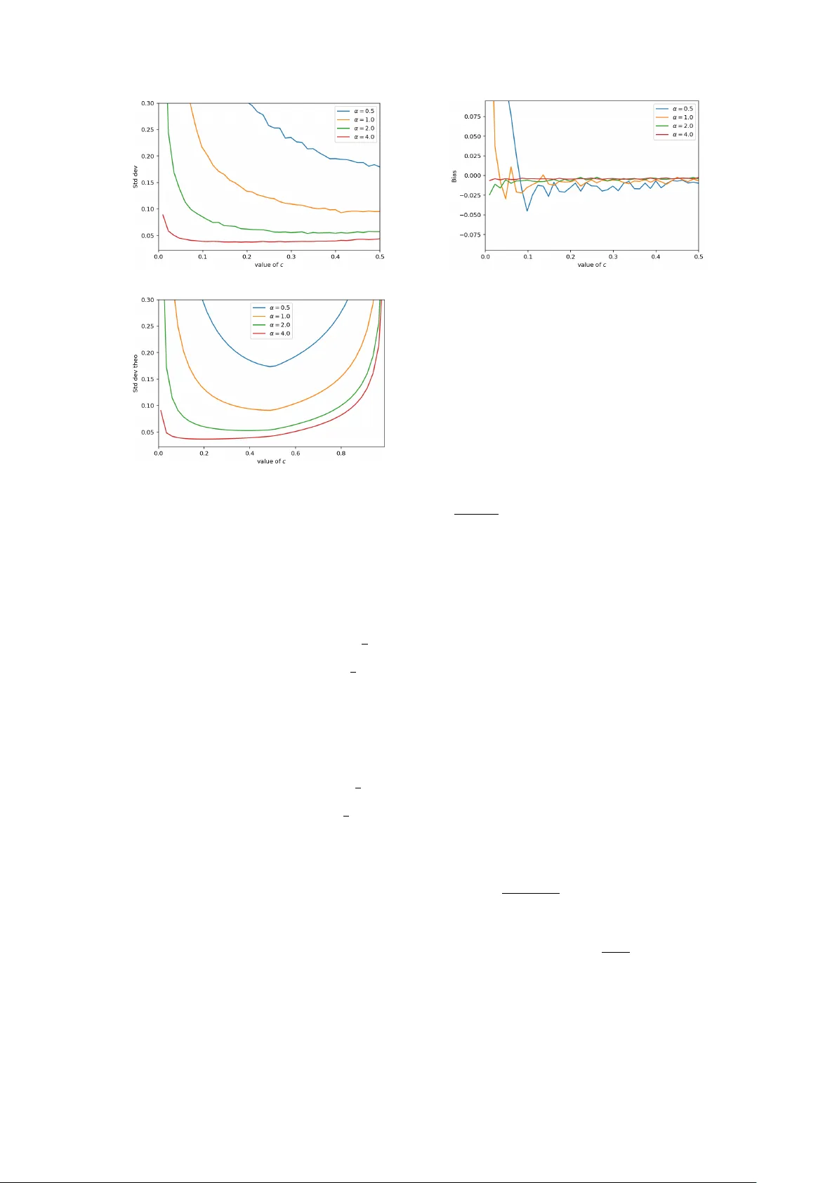
On the role of symmetry for staircase mec hanisms in lo cal differen tial priv acy efficiency across differen t priv acy regimes Chiara Amorino ∗ Arnaud Gloter † Marc h 31, 2026 Abstract W e inv estigate the structural foundations of statistical efficiency under α -local differential priv acy , with a fo cus on maximizing Fisher information. Building on the role of con tinuous staircase mec hanisms, w e iden tify a fundamen tal symmetry regarding the extremal v alues 1 and e α . W e demonstrate that when the optimal measure satisfies this symmetry , the Fisher information admits a close d-form expression. More generally , w e deriv e a decomposition of the Fisher information in to symmetric and asymmetric comp onents, scaling as α 2 and α 3 , resp ectiv ely , for α → 0 . This rev eals that, if in the high-priv acy regime asymmetry is negligible, it is no longer the case as priv acy constrain ts are relaxed. Motiv ated by this, w e in tro duce a class of fully asymmetric priv acy mec hanisms con- structed via pushforw ard mappings, pro ving that—unlike their symmetric coun terparts—they reco ver the full Fisher information of the non-priv ate mo del as α → ∞ . W e bridge the gap b et w een theory and practice by providing a tractable implementation of these mechanisms, go verned b y a tuning parameter c . This parameter allo ws for a smo oth in terp olation betw een the symmetric regime and the fully asymmetric regime. F urthermore, we demonstrate the v ersatility of this framew ork b y sho wing that it encompasses the binomial mechanism as a limiting case. K eywor ds: lo c al differ ential privacy, Fisher information, efficiency, stair c ase me chanism MSC2020 subje ct classific ations: Primary 62F12, 62F30; se c ondary 62B15 Con ten ts 1 In tro duction 2 2 Problem form ulation 4 2.1 The staircase mec hanism . . . . . . . . . . . . . . . . . . . . . . . . . . . . . . . . 5 2.2 P arametric models and Fisher information . . . . . . . . . . . . . . . . . . . . . . 8 3 Main results 9 3.1 Asymmetric priv acy mec hanisms . . . . . . . . . . . . . . . . . . . . . . . . . . . 13 3.2 Implemen tation of the method: from theory to practice . . . . . . . . . . . . . . 15 3.3 Appro ximation of binomial mec hanism . . . . . . . . . . . . . . . . . . . . . . . . 17 ∗ Univ ersitat P omp eu F abra and Barcelona School of Economics, Department of Economics and Business, Ramón T rias F argas 25-27, 08005, Barcelona, Spain. The author gratefully ackno wledges financial supp ort of PID2022-138268NB-I00/AEI/10.13039/501100011033. † Lab oratoire de Mathématiques et Mo délisation d’Evry , CNRS, Univ Evry , Univ ersité Paris-Sacla y , 91037, Evry , F rance. 1 4 Pro ofs 19 4.1 Pro of of Proposition 1 . . . . . . . . . . . . . . . . . . . . . . . . . . . . . . . . . 19 4.2 Pro of of Theorem 1 . . . . . . . . . . . . . . . . . . . . . . . . . . . . . . . . . . . 20 4.3 Pro of of Proposition 2 . . . . . . . . . . . . . . . . . . . . . . . . . . . . . . . . . 24 4.4 Pro of of Lemma 2 . . . . . . . . . . . . . . . . . . . . . . . . . . . . . . . . . . . 26 4.5 Pro of of Proposition 3 . . . . . . . . . . . . . . . . . . . . . . . . . . . . . . . . . 26 1 In tro duction W e ha v e en tered the era of big data, in whic h statisticians and data scien tists ha v e access to increasingly large and ric h datasets. The gro wing a v ailabilit y of data offers unpreceden ted opp ortunities for statistical analysis and inference. Ho wev er, a substan tial p ortion of these data are sensitive in nature, making it essen tial to ensure appropriate levels of priv acy protection. Sev eral approac hes to data priv acy hav e b een prop osed in the literature. Among them, differen tial priv acy has emerged as a fundamental and widely adopted framew ork. The notion of global differen tial priv acy , also referred to as cen tral differen tial priv acy , w as first in tro duced in the seminal w ork of Dwork et al. [10], where a trusted curator has access to the entire dataset and releases priv atized outputs. Lo cal differential priv acy , b y contrast, do es not rely on the existence of a trusted aggregator: eac h user priv atizes their data lo cally before transmission. This stronger priv acy model has b een adopted in practice by ma jor technology companies suc h as Apple [24, 23] and Go ogle [1, 11], highlighting the relev ance of lo cal differential priv acy b oth from a theoretical p ersp ectiv e and for real-w orld applications. While lo cal differen tial priv acy provides stronger priv acy guaran tees, it also entails a signif- ican t loss in statistical utility . This fundamental tension has motiv ated a growing b o dy of w ork dev oted to statistical inference under lo cal differential priv acy constraints. Early and influen tial con tributions in this direction include [8] and [26]. Within this line of research, particular atten- tion has b een given to parametric inference; see, for instance, [3, 4, 7, 15, 17]. A cen tral theme is moreov er the construction of statistically efficient estimators under priv acy constraints. Although a rigorous definition of lo cal differential priv acy is deferred to later in the pap er (see (2)), we highligh t here that the level of priv acy is con trolled b y a parameter α ∈ [0 , ∞ ) . The case α = 0 corresp onds to p erfect priv acy , whereas priv acy constraints b ecome progressiv ely w eaker as α → ∞ . As exp ected, stronger priv acy guarantees (i.e., smaller v alues of α ) lead to a reduction in statistical information, limiting the extent to which the statistician can exploit the data. This inherent priv acy–utility trade-off has motiv ated extensiv e researc h aimed at c haracterizing optimal priv acy levels and, for a fixed priv acy budget α , at iden tifying priv acy mec hanisms that ac hieve the b est p ossible statistical performance, according to a particular utilit y function that one aims at maximizing/minimizing. In this pap er, we fo cus on the latter problem. Sp ecifically , for a fixed level of priv acy α , we in vestigate the design of priv acy mechanisms that are optimal in the sense of maximizing the Fisher information. This optimalit y criterion has b een extensively studied in the literature and pla ys a central role in our analysis. In the context of central differen tial priv acy , the early w orks [20, 21] initiated the study of efficien t parameter estimation under priv acy constrain ts. In the lo cal differential priv acy setting, [5] deriv ed upp er bounds on the Fisher information ac hiev able under LDP , though without constructing explicit priv acy mechanisms attaining these b ounds. Subsequen t progress w as made b y [19], who inv estigated Fisher information maximization under one-bit communication sc hemes. More recently , several w orks hav e further adv anced the understanding of efficiency under LDP , including [9, 22, 2]. In particular, [9] introduced the notion of L 1 -information to c harac- terize the lo cal minimax risk of regular parametric mo dels under LDP , up to univ ersal constants. Recen tly , [22] established the existence of asymptotically efficient lo cally priv ate estimators and 2 pro vided explicit constructions achieving minim um v ariance by solving a contin uous optimiza- tion problem via a discretization approac h. Finally , [2] deriv ed an exact contin uous solution to the same optimization problem, thereb y eliminating the need for any discretization step. A cross these recent contributions, it has b ecome clear that staircase mechanisms—also re- ferred to as extremal mec hanisms—play a cen tral role in optimization problems under priv acy constrain ts (see Definition 1 for a precise definition). The one-dimensional staircase mec ha- nism was introduced b y [14], who sho wed b oth theoretically and empirically that its piecewise- constan t noise outp erforms the Laplace mechanism. This construction w as later extended to higher dimensions in [13], where the authors again demonstrated sup eriority o ver Gaussian and Laplace noise for d ≥ 2 . More recen tly , [18] prop osed a staircase-like scheme for one-dimensional mean estimation, while [16] form ulated the priv acy–utilit y trade-off as a constrained optimiza- tion problem and prov ed that, on finite spaces, the class of staircase mechanisms contains the exact optima for a broad family of information-theoretic utilit y criteria. Staircase mechanisms also play a crucial role in [22] and [17], where they are used to explicitly construct optimal pri- v acy mechanisms that attain the lo w er b ounds derived in the analysis, as well as in [27], whic h is devoted to discrete distribution estimation under utility-optimized lo cal differen tial priv acy . Moreo ver, related ideas ha v e b een emplo yed in [6] to construct gentle measurements, exploiting the connection b et w een gen tleness and differen tial priv acy . T o address non-discrete domains, [2] introduced the notion of contin uous staircase mech- anisms and established their effectiv eness for Fisher information maximization under LDP in infinite-dimensional settings. In that work, b oth upp er and low er b ounds on the Fisher informa- tion were derived in the con tinuous case, and it was sho wn that these b ounds coincide as α → 0 . Moreo ver, for fixed α , the maximization problem was shown to admit a solution: sp ecifically , there exists a Radon sub-probability measure ¯ µ on the set of extremal p oin ts E (see (9)) suc h that the asso ciated con tinuous staircase mec hanism q ( ¯ µ ) solv es the Fisher information maximiza- tion problem. The supp ort of ¯ µ is the set of lab els where the priv acy mec hanism outputs the public v ariables. Nevertheless, little is currently kno wn ab out the structure of the measure ¯ µ , or ab out the explicit form of the resulting priv acy mechanism and its Fisher information. This w ork builds on the observ ation that the structure of the set of extremal v alues—most notably the v alues 1 and e α —pla ys a fundamental role in determining the b eha vior of con tin- uous staircase mechanisms. This insight motiv ates our fo cus on measures that are in v arian t under swapping these extremal v alues. It is noticeable that the binomial priv acy mec hanisms, whic h are optimal for α → 0 , are associated to measures satisfying this symmetry prop ert y . W e demonstrate that a symmetrization pro cedure can b e used to construct a randomization mec hanism from any p ositiv e Radon measure on the set of extremal points E . Within this framew ork, binomial mec hanisms emerge as the sp ecial case where the underlying measure is a Dirac mass centered at a p oin t in E . W e show that, when the Radon sub-probability mea- sure ¯ µ solving the maximization problem satisfies this symmetry prop ert y , the asso ciated Fisher information admits a closed-form expression for any fixed α , and the mechanism reduces to a binomial mec hanism. This observ ation naturally leads us to study this form of symmetry in greater depth. In doing so, w e unco v er that even when the measure solving the optimization problem is not symmetric, the corresp onding Fisher information can still b e decomp osed into a symmetric and an asymmetric comp onen t. As to b e expected, the asymmetric comp onen t v anishes when the measure is symmetric, thus recov ering the previous result. More in terest- ingly we show that, in the asymptotic regime α → 0 , the symmetric comp onent scales as α 2 , whereas the asymmetric one is of order α 3 . As a consequence, in the high-priv acy regime, the con tribution of the asymmetric part b ecomes negligible. This phenomenon no longer holds for larger v alues of α , whic h provides one motiv ation for studying asymmetric priv acy mec hanisms in detail. Another motiv ation originates from practical considerations: general E -v alued priv acy mec hanisms can b e difficult to implemen t in practice. With this in mind, in Section 3.1 we analyze a class of asymmetric priv acy mec hanisms whose asso ciated measures on E are obtained 3 via a pushforw ard construction from probabilit y measures ν defined on the original alphabet X . In this wa y w e are able to implement a large class of priv acy mec hanisms indexed by ν . Notably , we sho w that, for such mec hanisms, taking the limit α → ∞ of the asso ciated Fisher information recov ers the same amoun t of information as in the absence of priv acy constrain ts. This is in sharp contrast with the b eha vior of symmetric t w o-p oin t mechanisms, for whic h suc h a recov ery do es not o ccur. T o bridge the gap b et ween these theoretical gains and practical utilit y , w e provide a concrete, implemen table algorithm for these mechanisms, introducing a tuning parameter c that con tinuously interpolates b et ween the symmetric ( c = 1 / 2 ) and fully asymmetric regimes. Numerical exp erimen ts on Gaussian translation mo dels confirm that while symmetry is optimal for strong priv acy , breaking symmetry by tuning c reduces v ariance in lo w-priv acy settings. Finally , we demonstrate the v ersatility of our framework by constructing a sp ecific asymmetric appro ximation that con v erges to the binomial mec hanism. This allows our con tinuous framework to seamlessly replicate the asymptotic optimality of discrete mechanisms as α → 0 , effectiv ely offering a unified approac h that remains efficien t across the en tire priv acy sp ectrum. The pap er is organized as follows. Section 2 establish es the mathematical framework, intro- ducing formal definitions for b oth discrete and contin uous extremal mechanisms. In Section 3, we presen t our main contributions, b eginning with a detailed analysis of symmetric priv acy mec hanisms and their optimality in the high-priv acy regime. This naturally leads to the study of asymmetric priv acy mec hanisms in Section 3.1, where w e demonstrate their adv antages as priv acy constraints are relaxed. W e then turn to practical applications in Sections 3.2 and 3.3, pro viding a concrete implemen tation of our metho d and dev eloping an asymmetric appro xima- tion of the binomial mec hanism. Finally , Section 4 contains the proofs of our main results. 2 Problem form ulation As already men tioned, this pap er focuses on efficiency under α -LDP constrain ts and aims to in vestigate the role of symmetry in this con text. The first step is to formally define local differen tial priv acy . The pro cess of transforming raw data into public data is mo deled through a conditional distribution, referred to as a priv acy mechanism or c hannel distribution. Sp ecifically , let X and Z be tw o separable, complete metric spaces. Equipped with their resp ectiv e Borel σ -algebras, they form the measurable spaces ( X , Σ X ) and ( Z , Σ Z ) . The first represen ts th e space of sensitiv e data to whic h the priv acy mechanism is applied. The resulting output Z liv es in ( Z , Σ Z ) , corresp onding to the space of priv atized (public) data. T o formalize the transformation of raw samples into public views, let X 1 , . . . , X n b e i.i.d. pri- v ate observ ations taking v alues in a domain X . While priv acy mechanisms generally fall in to tw o categories—in teractive and non-in teractive—this work focuses primarily on the non-in teractive setting. Ho wev er, for the sake of completeness, we first recall the definition of a sequentially in teractive mechanism. In this broader con text, the priv atization of the i -th observ ation allo ws for dep endency not only on the curren t priv ate datum X i , but also on the history of previously released public outpu ts Z 1 , . . . , Z i − 1 . This results in the follo wing conditional indep endence structure: X i , Z 1 , . . . , Z i − 1 → Z i , Z i ⊥ X k | X i , Z 1 , . . . , Z i − 1 for k  = i. Hence, the priv atized output Z i is drawn according to Z i ∼ Q i ( · | X i = x i , Z 1 = z 1 , . . . , Z i − 1 = z i − 1 ) , for a collection of Mark ov kernels Q i : Σ Z × X × Z i − 1 → [0 , 1] . In con trast, in the non-in teractive setting, the public v ariable Z i dep ends solely on the cor- resp onding ra w v alue X i and is independent of the previously generated v ariables Z 1 , . . . , Z i − 1 . 4 Consequen tly , the Mark ov k ernel Q do es not dep end on i , and the same mechanism is applied to all observ ations. Therefore, for each i ∈ { 1 , . . . , n } , the priv atized output is dra wn as Z i ∼ Q ( · | X i = x i ) . (1) Observ e that b oth in teractive and non-in teractiv e mec hanisms ha ve b een widely studied in the literature. On one hand, it is intuitiv e that working with non-in teractive mechanisms is simpler, since starting from indep endent ra w data results in indep enden t public data, which is not the case for interactiv e mec hanisms. On the other hand, the extra dependence in the interactiv e setting is due to the fact that eac h Z i carries not only information ab out X i but also ab out X 1 , . . . , X i − 1 , which can enhance statistical inference. What is imp ortan t in b oth cases is that the concept of lo cal differential priv acy allows us to quan tify the amoun t of priv acy injected into the system, through the parameter α . This naturally leads to the definition of α -lo cal differential priv acy . Given a parameter α ≥ 0 , we sa y that a random v ariable Z i is an α -lo cally differentially priv ate v ersion of X i if, for all z 1 , . . . , z i − 1 ∈ Z and all x, x ′ ∈ X , the follo wing condition holds: sup A ∈ Σ Z Q i  A | X i = x, Z 1 = z 1 , . . . , Z i − 1 = z i − 1  Q i  A | X i = x ′ , Z 1 = z 1 , . . . , Z i − 1 = z i − 1  ≤ exp( α ) . (2) Recall that we ha ve denoted by Q α the set of all Marko v kernels satisfying this lo cal α - differen tial priv acy constrain t. This set will play a central role, as our optimization problem will in volv e searching for the priv acy mec hanism within Q α that maximizes the Fisher information. In the non-in teractive case, the definition of α -LDP simplifies to sup A ∈ Σ Z Q ( A | X = x ) Q ( A | X = x ′ ) ≤ exp( α ) . W e underline that the parameter α quan tifies the strength of priv acy: the smaller the v alue, the harder it is to infer sensitiv e information from the released data. In particular, α = 0 corresp onds to perfect priv acy , while letting α → ∞ gradually relaxes the priv acy constraint. Under the lo cal differen tial priv acy condition, the kernels Q ( · | X = x ) are mutually ab- solutely contin uous for all x ∈ X . Therefore, we ma y assume the existence of a dominating measure µ on ( Z , Σ Z ) with respect to whic h each k ernel admits a densit y , denoted q ( x, z ) . The α -lo cal differential priv acy constraint can then b e rewritten in terms of these densities, giving rise to the following equiv alen t formulation, which will b e the one we use most frequently in the sequel: sup z ∈Z q ( x, z ) q ( x ′ , z ) ≤ exp( α ) , ∀ x, x ′ ∈ X . (3) In what follo ws, w e will write q ( x, z ) to denote the density q ( z | X = x ) . Finally , note that if q ( x, z ) = 0 for some x ∈ X and z ∈ Z , then the α -LDP constraint implies that q ( x ′ , z ) = 0 for all x ′ ∈ X . In other words, suc h a v alue z could b e remo v ed from Z without altering the randomization mec hanism. 2.1 The staircase mechanism Ha ving established the necessary background on data priv atization, w e now turn to the problem of efficient parameter estimation under α -LDP . This problem has b een widely in vestigated in the literature, as discussed in the in tro duction. In this context, staircase mec hanisms pla y a cen tral role. Before pro ceeding with our analysis, w e recall their definition in the finite-alphab et setting. A key reference on this topic is [16], which shows that when X is finite, the optimal mechanism maximizing utilit y functions expressible as sums of sublinear functions has an extremal structure. 5 W e will then briefly mention their extension to infinite-dimensional settings, as recently proposed in [2]. F ollo wing [16], a randomization mec hanism is called extremal if, for all z ∈ Z and all ( x, x ′ ) ∈ X 2 , the log-lik eliho o d ratios satisfy     ln q ( x ′ , z ) q ( x, z )     ∈ { 0 , α } , whic h is equiv alen t to the condition ∀ z ∈ Z , ∀ ( x, x ′ ) ∈ X 2 , q ( x ′ , z ) q ( x, z ) ∈ { e − α , 1 , e α } . (4) An y mec hanism satisfying this constraint is referred to as a staircase mechanism. One of the main reasons staircase mechanisms hav e b een so intensiv ely studied is that they saturate the α -LDP constraint, whic h naturally places them in a strong position for proving optimalit y in constrained optimization problems. In particular, the so-called staircase pattern matrix, as defined b elow, app ears naturally in suc h problems (see, e.g., Theorem 4 in [16] or Section 2.1.3 of [17]). Definition 1. F or β ∈ { 0 , . . . , 2 d − 1 } , let d j ( β ) denote the j -th c omp onent of the d -dimensional binary ve ctor c orr esp onding to the dyadic exp ansion of β , that is, β = d − 1 X j =0 d j ( β )2 j , with d j ( β ) ∈ { 0 , 1 } . A matrix is c al le d a stair c ase p attern matrix if its β -th c olumn is a ve ctor r β ∈ { 1 , e α } d for e ach β ∈ { 0 , . . . , 2 d − 1 } , wher e the j -th c omp onent of r β is define d by ( r β ) j = 1 { d j ( β )=0 } + e α 1 { d j ( β )=1 } . Each such c olumn ve ctor r β is c al le d a stair c ase p attern. T o clarify this construction, consider the case d = 3 . There are 2 d = 8 staircase patterns, and the corresp onding staircase pattern matrix is   1 1 1 1 e α e α e α e α 1 1 e α e α 1 1 e α e α 1 e α 1 e α 1 e α 1 e α   . This structure can b e describ ed for an y d in a general w a y b y introducing the following vectors r r 0 =        1 1 1 . . . 1        , r 1 =        e α 1 1 . . . 1        , r 2 =        1 e α 1 . . . 1        , . . . r 2 d − 1 =        e α e α e α . . . e α        . (5) One sees that the v ectors  r β  β ∈{ 0 ,..., 2 d − 1 } corresp ond to the extremal points of the h yp er- rectangle [ 1 , e α ] d . In the finite-dimensional case, one can define E = { 0 , . . . , 2 d − 1 } as the index set of these extremal patterns { r 0 , . . . , r 2 d − 1 } . In particular, if X has finite cardinality , sa y X = { x 1 , . . . , x d } , eac h r β can b e in terpreted as a function on X , with r β ( x j ) = ( r β ) j , for x j ∈ X . 6 F or each β ∈ E , the lev el sets F + β = { x ∈ X | r β ( x ) = e α } , F − β = { x ∈ X | r β ( x ) = 1 } (6) pla y a crucial role, so that for all x ∈ X , the function r β satisfies r β ( x ) = e α 1 F + β ( x ) + 1 F − β ( x ) = 1 +  e α − 1  1 F + β ( x ) , (7) i.e., the function r β tak es v alues in { 1 , e α } with its structure fully determined b y F + β . Since here we fo cus on the setting where X may b e con tin uous, w e rely on the extension of staircase mechanisms introduced in Section 3 of [2]. In this case, the hyper-rectangle [1 , e α ] d of the finite setting is replaced by the set B := ß v : X → R measurable     1 ≤ v ( x ) ≤ e α a.e. ™ ⊂ L ∞ ( X , R ) , (8) and the extremal p oin ts of [1 , e α ] d are replaced b y the extremal points of B , namely E := ß r : X → R measurable     r ( x ) ∈ { 1 , e α } a.e. ™ . (9) Analogously to the level sets in (6) and the associated v ectors in (7), for any r ∈ E we define F + r := r − 1  { e α }  , F − r := r − 1  { 1 }  , (10) so that dx -almost everywhere we can write r ( x ) = e α 1 F + r ( x ) + 1 F − r ( x ) = 1 +  e α − 1  1 F + r ( x ) . (11) Finally , note that w e equip B with the metric top ology of w eak- ⋆ con vergence and consider the asso ciated Borel σ -algebra B ( B ) , which mak es the set E measurable (see details in [2]). In this w ay , w e obtain a construction that provides the analogue of a staircase pattern, as in Definition 1, but now in the infinite-dimensional setting. Our goal is to lev erage this construction to describe an extremal (staircase) mechanism, with a particular fo cus on the symmetry of the asso ciated measures. T o do so, it is essen tial to ev aluate elemen ts of the set B at a p oin t x ∈ X , whic h motiv ates the introduction of the follo wing ev aluation operator: e : ® ( X × B , B ( X ) ⊗ B ( B )) → R , ( x, r ) 7→ e x ( r ) , whic h is measurable and satisfies, for all r ∈ B , e x ( r ) = r ( x ) for almost ev ery x . W e are no w ready to in tro duce extremal randomizations in the con tin uous setting. F or an y non-negativ e Borel measure µ on E satisfying for a.e. x ∈ X , Z E e x ( r ) µ ( dr ) = 1 , (12) w e define a randomization mechanism from X to E by means of the k ernel q ( µ ) ( x, dr ) = e x ( r ) µ ( dr ) . (13) The condition (12) is here crucial to ensure that the measure q ( µ ) ( x, dr ) defines a randomization on E for almost every x ∈ X . One can chec k that this randomization is extremal in the same sense as in (4), since q ( µ ) ( x, dr ) q ( µ ) ( x ′ , dr ) = e x ( r ) e x ′ ( r ) = r ( x ) r ( x ′ ) ∈ { e − α , 1 , e α } for a.e. dx dx ′ . Moreo ver, since e x ( r ) ∈ [1 , e α ] , condition (12) implies the b ounds e − α ≤ µ ( E ) ≤ 1 , (14) whic h will b e useful in the sequel. 7 2.2 P arametric mo dels and Fisher information In the follo wing, it will be crucial to w ork with models satisfying appropriate regularit y condi- tions. In this subsection, we b egin by detailing the notion of regularit y w e hav e in mind. Assume that X is an op en subset of R d and that ( P θ ) θ ∈ Θ is a family of probability measures on X , with Θ ⊂ R d Θ . W e suppose that this family is dominated by the Lebesgue measure, and denote its densit y b y p θ ( x ) := dP θ ( x ) dx . Let α > 0 and let µ b e a Radon sub-probabilit y measure on E satisfying (12). W e consider the asso ciated priv acy mec hanism q ( µ ) as introduced in (13), denote b y Z the corresp onding public data, and b y ( e P θ ) θ ∈ Θ the induced mo del on E , i.e., the law of Z . This model is regular in the sense of differen tiabilit y in quadratic mean. W e recall here the definition of differen tiability in quadratic mean (DQM) at an in terior point θ 0 ∈ ◦ Θ . Definition 2. A statistic al mo del P = ( P θ ) θ ∈ Θ , with Θ ⊂ R d Θ , sample sp ac e ( Y , G ) , and dominating me asur e ˜ µ , is said to b e differ entiable in quadr atic me an (DQM) at θ 0 ∈ ◦ Θ if the ˜ µ -densities p θ = dP θ dµ satisfy, for h ∈ R d Θ , Z X  » p θ 0 + h ( x ) − » p θ 0 ( x ) − 1 2 h ⊤ s θ 0 ( x ) » p θ 0 ( x )  2 ˜ µ ( dx ) = o ( ∥ h ∥ 2 ) as h → 0 , for some me asur able ve ctor-value d function s θ 0 : X → R d Θ , which is c al le d the sc or e at θ 0 . A mo del is said to b e DQM if it is DQM at every p oin t θ ∈ ◦ Θ . It will b e crucial for our pro ofs to note that if the mo del P is DQM at θ 0 , then its score function is cen tered, that is E θ 0  s θ 0  = 0 , (15) and the Fisher information exists, is finite, and tak es the form I θ 0 ( P ) = E θ 0  s θ 0 s ⊤ θ 0  . A pro of of these results can b e found in Theorem 7.2 of [25]. If one considers transformations of DQM models via Marko v channels satisfying lo cal dif- feren tial priv acy , Lemma 3.1 of [22] shows that if the original mo del ( P θ ) θ is DQM at θ 0 with dominating measure dx , then the priv atized mo del ( q ◦ P θ ) θ is also DQM at θ 0 with dominating measure µ . The score function of the latter is t θ 0 ( z ) = E [ s θ 0 ( X ) | Z = z ] = R X s θ 0 ( x ) q ( x, z ) p θ 0 ( x ) µ ( dx ) R X q ( x, z ) p θ 0 ( x ) µ ( dx ) . (16) Moreo ver, according to Lemma 1 of [2], the law of the public v ariable Z that is the induced mo del ( e P θ ) θ ∈ Θ on E , admits a contin uous density with respect to the reference measure µ e p θ ( r ) := d e P θ dµ ( r ) = Z X r ( x ) p θ ( x ) dx, (17) whic h is differentiable in quadratic mean and has an explicit contin uous score function t θ 0 ( r ) = R X s θ 0 ( x ) r ( x ) p θ 0 ( x ) dx e p θ 0 ( r ) = ( e α − 1) R F + r s θ 0 ( x ) p θ 0 ( x ) dx e p θ 0 ( r ) . (18) 8 This allows us to write the Fisher information explicitly: I θ 0  q ( µ ) ◦ P  = E θ 0 î t θ 0 ( Z ) t θ 0 ( Z ) ⊤ ó = Z E t θ 0 ( r ) t θ 0 ( r ) ⊤ e p θ 0 ( r ) µ ( dr ) = Z E ( R X s θ 0 ( x ) r ( x ) p θ 0 ( x ) dx ) ( R X s θ 0 ( x ) r ( x ) p θ 0 ( x ) dx ) ⊤ e p θ 0 ( r ) µ ( dr ) (19) = ( e α − 1) 2 Z E Ä R F + r s θ 0 ( x ) p θ 0 ( x ) dx ä Ä R F + r s θ 0 ( x ) p θ 0 ( x ) dx ä ⊤ e p θ 0 ( r ) µ ( dr ) . With all this bac kground in place, we are finally ready to discuss the optimization problem for the Fisher information, which consists of searching for the priv acy mec hanism achieving maximal Fisher information. This search for the optimal priv acy mechanism q ( µ ) can b e rephrased as lo oking for the optimal measure µ asso ciated with such a mec hanism. Let us consider the case where the parameter θ 0 is one-dimensional, and define, for an y r ∈ B , i ( r ) := ( R X s θ 0 ( x ) r ( x ) p θ 0 ( x ) dx ) 2 R X r ( x ) p θ 0 ( x ) dx = ( e α − 1) 2 Ä R F + r s θ 0 ( x ) p θ 0 ( x ) dx ä 2 1 + ( e α − 1) R F + r p θ 0 ( x ) dx , (20) where we hav e used (11). This leads to the following optimization problem: I ∗ := sup µ Z E i ( r ) µ ( dr ) , sub ject to Z E e x ( r ) µ ( dr ) = 1 for dx -almost ev ery x, (21) where the suprem um is taken ov er all Radon sub-probabilit y measures µ on E . F rom Theorem 2 of [2], we kno w that this optimization problem admits a solution, i.e., there exists a Radon sub-probability measure µ on E suc h that the mec hanism defined b y q ( µ ) ( x, dr ) := e x ( r ) µ ( dr ) satisfies J max ,α θ 0 = I θ 0 Ä q ( µ ) ◦ P ä . Although the existence of a priv acy mechanism solving this optimization problem is guaranteed, little can b e said ab out its explicit form. The main purpose of this paper is to in vestigate in greater detail this optimal Fisher infor- mation and to gain insigh ts into the priv acy mec hanism ac hieving it. In particular, w e will see that by in tro ducing a notion of symmetry for the optimal measure, further structural insights can b e obtained. 3 Main results F rom the bac kground dev elop ed in the previous section, it is clear that the structure of the set E pla ys a central role in the b ehavior of the Fisher information and on the definition of the priv acy mec hanism. In b oth the discrete and contin uous settings, the extremal v alues 1 and e α emerge as particularly significant. This naturally raises the question: can the analysis b e simplified b y considering measures on E that are, in some sense, indifferent to the distinction betw een these t wo v alues? Can this help to construct normalized Radon measures µ on E ? T o formalize this idea, let us consider Radon measures µ on E satisfying the normalization condition Z E e x ( r ) µ ( dr ) = 1 for a.e. dx, 9 and let us introduce the op erator T : E → E defined b y T ( r ) := e α + 1 − r, (22) whic h essentially sw aps the v alues 1 and e α : for each x , we ha ve T ( r )( x ) = 1 if and only if r ( x ) = e α . This op erator captures a natural form of symmetry with respect to the extremal v alues in E . Given a Radon measure µ on E , w e define the pushforw ard measure T ( µ ) b y T ( µ ) := µ ◦ T , so that for any integrable function g on E , Z E g ( r ) T ( µ )( dr ) = Z E g ( T ( r )) µ ( dr ) . W e b egin b y introducing the formal notion of symmetry that serv es as a cornerstone for this w ork. Definition 3. L et µ b e a R adon me asur e on E satisfying the normalization c ondition (12) . W e say that µ is symmetric if it is invariant under the tr ansformation T , i.e., µ = T ( µ ) . Although symmetry is defined via T -in v ariance, it is important to observ e that T ( µ ) does not, in general, satisfy the normalization condition. T o see this, w e compute: Z E e x ( r ) T ( µ )( dr ) = Z E T ( e x ( r )) µ ( dr ) = Z E  e α + 1 − e x ( r )  µ ( dr ) = ( e α + 1) µ ( E ) − Z E e x ( r ) µ ( dr ) . This discrepancy suggests that an y arbitrary measure must b e appropriately transformed to satisfy b oth symmetry and normalization sim ultaneously . As it turns out, an y Radon mea- sure µ —irresp ectiv e of its initial prop erties—can b e mapp ed to such a state via the following construction: µ ( s ) := 1 ( e α + 1) µ ( E )  µ + T ( µ )  . (23) The fact that µ ( s ) is b oth normalized and symmetric (in the sense of Definition 3) is established in the follo wing proposition, the pro of of whic h is pro vided in Section 4. Prop osition 1. L et µ b e a R adon me asur e on E , and define µ ( s ) as in (23) . Then the fol lowing statements hold: 1. The me asur e µ ( s ) is normalize d in the sense of (12) and symmetric in the sense of Defi- nition 3. 2. If the original me asur e µ is alr e ady symmetric (i.e., µ = T ( µ ) ) and normalize d, then µ ( E ) = 2 e α +1 , and we r e c over µ ( s ) = µ . Remark 1. It is worth emphasizing that the c onstruction of µ ( s ) is entir ely self-c orr e cting. The symmetry and normalization pr op erties ar e enfor c e d by the op er ator T and the choic e of the denominator in (23) , r e gar d less of whether the initial me asur e µ p ossesses any sp e cific structur e or even a unit mass. 10 Observ e that, in the discrete setting, a key role is play ed by the t w o particular level sets: F + max := { x ∈ X : s θ 0 ( x ) > 0 } and F ′ + max := { x ∈ X : s θ 0 ( x ) < 0 } . These sets are crucial b ecause, in the n umerator of the Fisher information, the following quan tity app ears (see Equation (19)): Å Z X s θ ( x ) 1 F + r ( x ) p θ ( x ) dx ã 2 ≤ Å 1 2 Z X | s θ ( x ) | p θ ( x ) dx ã 2 = Å 1 2 E  | s θ ( X ) |  ã 2 , with equality if F + r = F + max or F + r = F ′ + max . Among the collection of sets ( F + r ) r ∈E in tro duced in (6), one can denote by r max and r ′ max the indices corresp onding to F + max and F ′ + max , resp ectiv ely . These provide natural candidates for the supp ort of a solution to the optimization problem in the discrete case (see Remark 3 in [2] for further details). In particular, Prop osition 7 of [2] uses this insight to establish an upp er b ound for the Fisher information, with a pro of that is quite technical, sho wing that the maximum of the optimization problem is indeed attained b y a sub-probabilit y measure supp orted on the set { r max , r ′ max } . Prop osition 8 of [2] is then devoted to proving a low er b ound, and in particular explicitly constructs a priv acy mechanism achieving this (optimal) Fisher information, based on the these t wo p oin ts. Remark 2. It is worth noting that the two-p oint me asur es discusse d ab ove, c ommonly use d to establish the lower b ound, il lustr ate the p ower of the symmetrize d me asur e µ ( s ) . Inde e d, these ar e obtaine d by symmetrizing the natur al ly pr op ose d choic e µ = δ r , with r = 1 + ( e α − 1) 1 F + max wher e F + max is as define d ab ove. In Pr op osition 7 of [2], we establish that this two p oints sym- metric me asur e is optimal in a setting of a finite set X as so on as α is smal l enough. A lso, [17] gives an example of two p oints symmetric me chanism optimal when X = R . The previously established Prop osition 1 enables the construction of a wide class of normal- ized and symmetric measures on E , which in turn yield a v ariet y of symmetric randomization mec hanisms. The next result illustrates why suc h symmetry is particularly useful for our anal- ysis: when the maximizer µ of the optimization problem (21) (whose existence is guaranteed by Theorem 2 of [2]) is symmetric, the corresponding Fisher information attains an explicit and simplified expression. T o state this result, we first introduce a conv enien t notation. Recall the function i ( r ) defined in (20). Then, following the construction of the symmetrized measure µ ( s ) in (23), we define the symmetrized version of i as: i ( s ) ( r ) := 1 2 [ i ( r ) + i ( T ( r ))] . (24) This quantit y pla ys a cen tral role in simplifying the expression of the Fisher information under symmetry , as detailed in the theorem below. Theorem 1. A ssume that the maximizer ¯ µ of the optimization pr oblem (21) is symmetric in the sense of Definition 3. Then, the function r 7→ i ( s ) ( r ) is ¯ µ -almost everywher e c onstant, and the maximum Fisher information is given by J max ,α θ 0 = 2 e α + 1 (max r ∈ B i ( s ) ( r )) , with i ( s ) ( r ) = ( e α − 1) 2 2 ( R F + r s θ 0 ( x ) p θ 0 ( x ) dx ) 2 ( e α − ( e α − 1) R F + r p θ 0 ( x ) dx )(1 + ( e α − 1) R F + r p θ 0 ( x ) dx ) . (25) 11 W e w ould like to compare our results on the maximal Fisher information with those previ- ously established in the literature. How ev er, very little is known ab out the form of the maximal Fisher information when the set X is infinite, apart from the existence of a solution. This moti- v ates us to compare our explicit findings with results from the discrete setting, esp ecially given that several similarities are immediately apparen t. When comparing the expression ab o v e with Theorem 1 in [2], multiple parallels can b e dra wn. In particular, as discussed earlier, the numerator of the function w e aim to maximize is alw ays b ounded ab o ve by Å 1 2 Z X | s θ 0 ( x ) | p θ 0 ( x ) dx ã 2 = Å 1 2 E  | s θ 0 ( X ) |  ã 2 , with equality holding if and only if F + r = F + max or F + r = F ′ + max . This prop ert y also app ears in the optimization problem for the finite setting. An imp ortant difference with resp ect to the discrete case, how ev er, lies in the structure of the index set E . In the discrete setting, E = { 0 , . . . , 2 d − 1 } is finite, whic h mak es it p ossible to explicitly verify that the solution to the optimization problem is supported on only t w o points, b y c hecking that the supp ort of the optimal sub-probability vector has cardinalit y betw een 1 and 2 d . In con trast, in the contin uous setting considered here, we ha ve |E | = ∞ , making suc h a v erification no longer feasible. As a consequence, we cannot rigorously confirm that the candidate iden tified by maximizing the numerator indeed solves the optimization problem, without a more delicate analysis of the denominator. Remark 3. Even without the detaile d analysis of the denominator just discusse d, the r esult ab ove highlights that if the optimal solution to the Fisher information maximization pr oblem is symmetric, then an optimal me chanism c an always b e c onstructe d as a binary me chanism. Inde e d, it is establishe d in the pr o of of The or em 1 that a maximizer of r ∈ B 7→ i ( s ) ( r ) exists in E ⊂ B . T aking ¯ r ∈ E such maximizing value, we c an c onsider ˜ µ = 1 1+ e α  δ ¯ r + δ T ( ¯ r )  which is a symmetric and normalize d me asur e. Then, the Fisher information of q ˜ µ is 2 e α +1 i ( s ) ( ¯ r ) and thus e qual to J max ,α θ 0 . Theorem 1 provides a simplified expression for the Fisher information in the case where the solution measure to the optimization problem (21) is symmetric. How eve r, this symmetry assumption does not alwa ys hold. In what follows, w e presen t a decomp osition of the Fisher information into symmetric and asymmetric comp onen ts. Before stating the result, let us in tro- duce the notation for the asymmetric parts of the measure µ ( as ) := µ − µ ( s ) . With this notation, the follo wing proposition holds (see Section 4 for the pro of ). Prop osition 2. L et µ b e a R adon me asur e satisfying the normalization c ondition (12) . Then, the Fisher information c an b e de c omp ose d as I θ 0 ( q ( µ ) ◦ P ) = Z E i ( s ) ( r ) µ ( dr ) + Å e α + 1 2 − 1 µ ( E ) ã 2 µ ( E ) Z E i ( s ) ( r ) µ ( dr ) − 2( e α − 1) µ ( E ) Z E i ( as ) ( r ) µ ( dr ) , wher e i ( as ) ( r ) := i ( s ) ( r ) Å Z F + r p θ 0 ( x ) dx − 1 2 ã . The notation ( as ) stands for "asymmetric", sinc e this quantity satisfies the antisymmetry r elation i ( as ) ( T ( r )) = − i ( as ) ( r ) . Mor e over, as α → 0 , the Fisher information admits the exp ansion I θ 0 ( q ( µ ) ◦ P ) = α 2 Z E Å Z F + r s θ 0 ( x ) p θ 0 ( x ) dx ã 2 µ ( dr ) + O ( α 3 ) . 12 Remark 4. A s exp e cte d, if the solution me asur e is symmetric, we r e c over the r esult of The or em 1, which c orr esp onds pr e cisely to the first term in the de c omp osition ab ove. Inde e d, in this c ase, we have µ ( E ) = 2 e α +1 by Point 2 of Pr op osition 1, and the same pr op osition guar ante es that µ = µ ( s ) . Mor e over, sinc e i ( as ) ( T ( r )) = − i ( as ) ( r ) and by the definition (23) of the symmetrize d me asur e µ ( s ) , we obtain: Z E i ( as ) ( r ) µ ( s ) ( dr ) = Z E 1 2 î i ( as ) ( r ) + i ( as ) ( T ( r )) ó µ ( dr ) = 0 . This shows that b oth the se c ond and thir d terms in the de c omp osition vanish when the me asur e is symmetric. Remark 5. In sc enarios wher e the data ar e highly sensitive and thus a high level of privacy is r e quir e d — c orr esp onding to the r e gime α → 0 — the asymmetric c ontribution to the Fisher information b e c omes ne gligible c omp ar e d to the symmetric one. Inde e d, the le ading term in the de c omp osition, c orr esp onding to the symmetric c ontribution, is of or der α 2 , as se en in the asymp- totic exp ansion. The r emaining two terms, which c aptur e the asymmetric c ontribution, also in- volve inte gr als of or der α 2 , but ar e multiplie d by pr efactors of or der α , namely Ä e α +1 2 − 1 µ ( E ) ä and e α − 1 . A s a r esult, their over al l c ontribution b e c omes of or der α 3 , and is ther efor e ne gligible in the limit α → 0 . This final observ ation motiv ates our fo cus on symmetric measures. In the high-priv acy regime, whic h is the most relev an t from an applied p ersp ectiv e, the Fisher information is dom- inated by its symmetric component, while the contribution of the asymmetric part v anishes asymptotically . This behavior no longer holds in the lo w-priv acy regime, corresp onding to large v alues of α . As detailed in the next section, whic h is dev oted to the analysis of asymmetric priv acy mec hanisms, asymmetry plays a non-negligible role. 3.1 Asymmetric priv acy mec hanisms F or large v alues of α , neglecting the asymmetric part of the measure to fo cus solely on the symmetric comp onen t no longer app ears to b e an appropriate approach. T o emphasize this, w e no w prop ose to analyze a purely asymmetric case, corresponding to a mo dified v ersion of the staircase mec hanism whic h presen ts p eaks centered around x . W e assume that X = R and construct the mechanism as follows. First, w e consider t wo increasing functions g : R → {−∞} ∪ R and d : R → R ∪ {∞} suc h that g ( x ) < d ( x ) . W e define the mapping I : ß X → E x 0 7→ I ( x 0 ) = r x 0 , (26) where the function r x 0 is the elemen t of E defined b y r x 0 : ß R → { 1 , e α } x 7→ r x 0 ( x ) = 1 + ( e α − 1) 1 [ g ( x 0 ) ,d ( x 0 )] ( x ) . (27) Note that the functions r x 0 tak e the constant v alue 1 across the entire space X , except in a the in terv al of R defined by [ g ( x 0 ) , d ( x 0 )] , where their v alue rises to e α . Remark that when an edge of the interv al is not finite, g ( x 0 ) = −∞ or d ( x 0 ) = ∞ , the in terv al should b e considered op ened at this edge. Let ν b e a probability measure on X that is absolutely contin uous with resp ect to the Leb esgue measure, i.e. it admits a densit y: ν ( dx ) = ν ( x ) dx . Define µ 0 on E as the pushforward of ν through the map I , that is, µ 0 = I # ν . Hence, for any measurable function f : E → R , Z E f ( r ) µ 0 ( dr ) = Z X f  I ( x 0 )  ν ( x 0 ) dx 0 . (28) 13 Observ e that, in general, µ 0 do es not satisfy the normalization condition (12). How ev er, in some cases, it is p ossible to rescale it and thereby in tro duce a new probability measure satisfying it. Let us explain b elo w which conditions on g and d are sufficient in order to rescale the measure µ 0 in to a normalized measure according to definition (12). First, w e assume that g is left con tinuous while d is righ t con tinuous on R and that g tak es the v alue −∞ on some interv al ( −∞ , x ∗ g ] and that d tak es the v alue ∞ on some in terv al [ x ∗ d , ∞ ) . W e define the inv erses of the functions g and d as follows: g − 1 ( x ) = sup { y ∈ R | g ( y ) ≤ x } , d − 1 ( x ) = inf { y ∈ R | d ( y ) ≥ x } . With these definitions, and using left (resp. right) con tinuit y of g (resp. d ), w e ha ve for all ( x, x 0 ) ∈ R 2 1 { g ( x 0 ) ≤ x ≤ d ( x 0 ) } = 1 { d − 1 ( x ) ≤ x 0 ≤ g − 1 ( x ) } . (29) Lemma 1. L et c ∈ (0 , 1) and assume that Z g − 1 ( x ) d − 1 ( x ) ν ( x 0 ) dx 0 = c (30) for al l x ∈ R . Define µ := µ 0 1 + ( e α − 1) c . Then, the me asur e µ satisfies the c ondition (12) . Pr o of. F or x ∈ R , w e write Z E e x ( r ) µ 0 ( dr ) = Z X e x  I ( x 0 )  ν ( x 0 ) dx 0 , having used (28), = Z X r x 0 ( x ) ν ( x 0 ) dx 0 , from the definition of I , = Z X  1 + ( e α − 1) 1 [ g ( x 0 ) ,d ( x 0 )] ( x )  ν ( x 0 ) dx 0 , where w e used (27), = 1 + ( e α − 1) Z X 1 [ g ( x 0 ) ,d ( x 0 )] ( x ) ν ( x 0 ) dx 0 . F rom (29), and R g − 1 ( x ) d − 1 ( x ) ν ( x 0 ) dx 0 = c , we deduce Z E e x ( r ) µ 0 ( dr ) = 1 + ( e α − 1) Z X 1 [ d − 1 ( x ) ,g − 1 ( x )] ( x 0 ) ν ( x 0 ) dx 0 = 1 + ( e α − 1) c. This show that µ = µ 0 / (1 + ( e α − 1) c ) satisfies the renormalization condition (12). W e now prop ose a construction of the tw o functions g and d suc h that Lemma 1 applies. Assume that ν ( x ) > 0 for all x ∈ R and set Ξ( x ) = R x −∞ ν ( y ) dy . W e fix c ∈ (0 , 1) . W e define the functions g c and d c as follows g c ( x ) = ® −∞ if x ≤ x ∗ g ,c := Ξ − 1 ( c ) Ξ − 1 ( − c 2 + Ξ( x )) if x > x ∗ g ,c (31) d c ( x ) = ® Ξ − 1 ( c 2 + Ξ( x )) if x < x ∗ d,c := Ξ − 1 (1 − c ) ∞ if x ≥ x ∗ d,c (32) These functions are increasing and with g c ( x ) < d c ( x ) for all x , as Ξ − 1 is strictly increasing on (0 , 1) and c > 0 . By definition g c is left con tin uous and d c is right con tinuous. The next lemma states that these functions satisfy the constrain t in (30). Its proof can b e found in Section 4 14 Lemma 2. W e have for al l x ∈ R , Z g − 1 c ( x ) d − 1 c ( x ) ν ( x 0 ) dx 0 = c. No w, we consider the measure µ 0 defined through µ 0 = I # ν , where we recall the definition of the mapping I in (26)–(27), with the choice of function g and d given by (31)–(32). Using Lemmas 1 – 2 the measure µ 0 can b e rescaled to define the measure on E µ := µ 0 1 + ( e α − 1) c , (33) whic h satisfies the normalization condition R E e x 0 ( r ) µ ( dr ) = 1 . The asso ciated priv acy mec ha- nism q ( µ ) ( x, dr ) := e x ( r ) µ ( dr ) can thus b e rewritten as q ( µ ) ( x, dr ) = e x ( r ) µ 0 ( dr ) 1 + ( e α − 1) c . (34) The follo wing prop osition sho ws that this construction yields an asymptotically efficien t mec hanism in the regime where α → ∞ and c → 0 , up to ask some regularit y on the mo del and on ν 0 . Assumption 1. W e assume that statistic al mo del ( P θ ) θ ∈ Θ is differ entiable in quadr atic me an (DQM) at θ 0 . Mor e over we assume that x 7→ p θ 0 ( x ) and x 7→ s θ 0 ( x ) ar e c ontinuous at almost every p oint x ∈ R . W e assume that ν is a c ontinuous function. Prop osition 3. Supp ose that A ssumption 1 holds true. Then, for the privacy me chanism q ( µ ) define d in (34) , we have I θ 0  q ( µ ) ◦ P  − → Z X ˙ p θ 0 ( x ) 2 p θ 0 ( x ) dx as c → 0 , ce α → ∞ . Remark 6. 1. The privacy me chanism (34) is asymmetric, and typic al ly µ and T ( µ ) have disjoint supp ort. 2. This r andomization pr o c e dur e enc o des the information on the private data x 0 thr ough the c onstruction of the function r x 0 , which exhibits a p e ak c enter e d ar ound x 0 which shifts with x 0 . 3. In a simpler c ontext wher e X = R / Z ∼ [0 , 1) is the torus and ν is uniform on [0 , 1) , we c an cho ose g ( x ) = x − c/ 2 and d ( x ) = x + c/ 2 and define µ 0 = I ♯ ( ν ) , c onsidering al l functions on X as 1 -p erio dic. Then, it is p ossible, along the lines of the pr o of of L emma 1, to che ck that the me asur e µ 0 define d in (33) satisfies (12) . A ctual ly, the c onstruction ab ove extends this example to the r e al line X = R and al lows the choic e of a gener al pr ob ability me asur e ν 0 . 3.2 Implemen tation of the metho d: from theory to practice W e no w turn to the practical application of the priv acy mec hanisms in tro duced in Section 3.1. While the theoretical construction of the measure q ( µ ) ( x, dr ) in (13) ma y app ear abstract, w e sho w here that it yields a concrete, implementable algorithm. Our strategy relies on transforming the abstract output space E in to a manageable, finite- dimensional representation. W e define the image of our mapping as b E = { I ( x 0 ) | x 0 ∈ R } ⊂ E . A central feature of our construction is the parameter c , which acts as a tuning knob for the mec hanism’s behavior. First, we ensure that our mapping preserv es the data structure. 15 Lemma 3. F or any privacy level α > 0 , if we cho ose the tuning p ar ameter c ≤ 1 / 2 , the map I : X → b E is one-to-one. Pr o of. F or an y x 0 ∈ R , the function I ( x 0 ) is defined as x 7→ 1 + ( e α − 1) 1 [ g c ( x 0 ) ,d c ( x 0 )] ( x ) . Injectivit y is guaranteed if the in terv al b oundaries g c ( x 0 ) and d c ( x 0 ) uniquely iden tify x 0 . F rom definitions (31)–(32), and giv en that the base measure ν > 0 , the functions x 0 7→ g c ( x 0 ) and x 0 7→ d c ( x 0 ) are strictly increasing where finite. Crucially , for c ≤ 1 / 2 , at least one boundary is alw ays finite, ensuring that the pair ( g c ( x 0 ) , d c ( x 0 )) uniquely reco vers x 0 . F rom this point forward, w e fix c ≤ 1 / 2 . By the Lusin-Souslin theorem, b E is a Borel set and I − 1 is measurable, allo wing us to pull bac k the randomized v alue into the data space X . W e define the probability measure on X as b q ( µ ) ( x, dx 0 ) = I − 1 ♯ ( q ( µ ) ( x, dr )) . W e can derive the explicit density of this mechanism. F or any test function f , the integral transformation yields: Z R f ( x 0 ) b q ( µ ) ( x, dx 0 ) = Z R f ( x 0 ) I − 1 ♯ ( q ( µ ) ( x, dr ))( dx 0 ) = Z b E f ( I − 1 ( r )) b q ( µ ) ( x, dr ) = Z b E f ( I − 1 ( r )) e x ( r ) µ 0 ( dr ) 1 + c ( e α − 1) , from (34), = Z X f ( I − 1 ( I ( x 0 ))) e x ( I ( x 0 )) ν ( x 0 ) dx 0 1 + c ( e α − 1) , as µ 0 = I ♯ ( ν ) , = Z X f ( x 0 )  1 + ( e α − 1) 1 [ g c ( x 0 ) ,d c ( x 0 )] ( x )  ν ( x 0 ) dx 0 1 + c ( e α − 1) , where w e used the expression of the function I ( x 0 ) ∈ E and the fact that e x is the ev alua- tion op erator at x . Recalling (29), we find the following explicit expression for density of the randomization mechanism, when c ≤ 1 / 2 , b q ( µ ) ( x, dx 0 ) dx 0 = Ä 1 + ( e α − 1) 1 [ d − 1 c ( x ) ,g − 1 c ( x )] ( x 0 ) ä ν ( x 0 ) 1 + c ( e α − 1) . (35) The structure of (35) suggests a straightforw ard implemen tation using rejection sampling with prop osal densit y ν . Relative to the proposal ν , the mechanism outputs public data x 0 more frequen tly when it falls within the in terv al [ d − 1 c ( x ) , g − 1 c ( x )] , whic h contains the priv ate data x . As c → 0 , this high-probabilit y in terv al shrinks to the singleton { x } , minimizing noise; con versely , as c increases, the interv al widens, increasing priv acy . If the priv ate data follows a density p θ ( x ) with cum ulative distribution function F θ , the resulting density of the public output b p θ ( x 0 ) is derived by integrating o ver the priv ate data distribution: b p θ ( x 0 ) = Z R b q ( µ ) ( x, dx 0 ) dx 0 p θ ( x ) dx = ν ( x 0 ) 1 + c ( e α − 1) [1 + ( e α − 1)( F θ ( d c ( x 0 )) − F θ ( g c ( x 0 )))] , ha ving used (35) and (29). Remark 7. W e r estrict our implementation to c ≤ 1 / 2 for a critic al r e ason: information c ol lapse, as discusse d in the fol lowing items. • L oss of inje ctivity: when c > 1 / 2 , the mapping I is no longer one-to-one. F or a wide r ange of c entr al data values (sp e cific al ly x 0 ∈ (Ξ(1 − c ) , Ξ( c )) ), the me chanism outputs a single c onstant I ( x 0 ) = r := 1 + ( e α − 1) 1 R . Effe ctively, the me chanism b e c omes "blind," failing to distinguish b etwe en any data p oints in this r e gion. 16 (a) Standard deviation (b) Bias (c) Theoretical standard deviation Figure 1: ν ( x ) = 1 √ 2 π e − x 2 / 2 • Statistic al c ost: this structur al c ol lapse destr oys utility. Be c ause the "blind sp ot" c arries zer o Fisher information ( i ( r ) = 0 ), the over al l information of the me chanism dr ops signif- ic antly. • Numeric al c onfirmation: as shown in Figur es 1c – 2c, the standar d deviation incr e ases im- me diately when c exc e e ds 1 / 2 . Thus, c = 1 / 2 r epr esents the structur al b oundary for the optimality of this metho d. T o assess the impact of the tuning parameter c and the density ν , w e simulate a Gaussian translation mo del X ∼ N ( θ , 1) with θ 0 = 0 using n = 10 3 observ ations and 2 × 10 3 Mon te Carlo trials. W e test t wo prop osal measures ν : a standard Gauss ian and a Cauch y distribution. As illustrated in Figures 1 – 2, the theoretical standard deviation increases significantly for c ≥ 1 / 2 ; consequen tly , w e restrict our analysis to the efficient regime c ∈ (0 , 1 / 2] where empirical results p erfectly matc h theoretical predictions. Our sim ulations reveal a clear transition in optimality based on the p riv acy level: in the high-priv acy regime ( α ≤ 1 ), the choice c = 1 / 2 minimizes v ariance, as low er v alues of c yield negligible Fisher information. Conv ersely , in the low-priv acy regime ( α large), efficiency requires asymmetry; for example, at α = 4 with a Gaussian ν , the minimal standard deviation of 3 . 67 × 10 − 2 is ac hieved at c ≃ 0 . 2 , a result that closely approac hes the non-priv ate MLE b enc hmark of 3 . 16 × 10 − 2 . 3.3 Appro ximation of binomial mechanism T o bridge the gap b et ween the mec hanism of Section 3.1 (optimal for low priv acy) and the binomial mechanism (kno wn to b e asymptotically optimal for high priv acy , α → 0 ), we in tro duce a modified construction that seamlessly interpolates b et ween these tw o regimes. By adjusting the parameter c , this generalized mechanism can transition from high-precision local estimation to a coarse binary classification. W e assume a unimodal lo cation mo del where the score function’s sign partitions the space into positive and negative half-lines, sp ecifically F + max = (0 , ∞ ) and F ′ + max = ( −∞ , 0) . W e assign p ositiv e densities ν + and ν − to these domains, with resp ectiv e 17 (a) Standard deviation (b) Bias (c) Theoretical standard deviation Figure 2: ν ( x ) = 1 π (1+ x 2 ) cum ulative distribution functions Ξ + ( x ) = R x 0 ν + ( y ) dy and Ξ − ( x ) = R x −∞ ν − ( y ) dy . T o construct the mechanism, we define the b oundary functions for x > 0 as g + c ( x ) = ® 0 if x ∈ (0 , (Ξ + ) − 1 ( c )] (Ξ + ) − 1 ( − c 2 + Ξ + ( x )) if x ∈ ((Ξ + ) − 1 ( c ) , ∞ ) d + c ( x ) = ® (Ξ + ) − 1 ( c 2 + Ξ + ( x )) if x ∈ (0 , (Ξ + ) − 1 (1 − c )) + ∞ if x ∈ [ (Ξ + ) − 1 (1 − c ) , ∞ ) and symmetrically for x < 0 , g − c ( x ) = ® −∞ if x ∈ ( −∞ , (Ξ − ) − 1 ( c )] (Ξ − ) − 1 ( − c 2 + Ξ − ( x )) if x ∈ ((Ξ − ) − 1 ( c ) , 0) d − c ( x ) = ® (Ξ − ) − 1 ( c 2 + Ξ − ( x )) if x ∈ ( −∞ , (Ξ − ) − 1 (1 − c )) 0 if x ∈ [ (Ξ − ) − 1 (1 − c ) , 0) . By defining the interv al boundaries g c ( x 0 ) and d c ( x 0 ) as the sup erp osition of these p ositiv e and negative comp onen ts, we construct the measure µ = I ♯ ( ν + + ν − 2+ c ( e α − 1) ) , which we verify satisfies the normalization condition (12). The crucial feature of this construction is its limit b eha vior: as c → 1 , the noise in terv als ( g ± c , d ± c ) expand to fill the en tire half-lines (0 , ∞ ) and ( −∞ , 0) . Consequen tly , the measure µ conv erges to the symmetric binomial measure 1 1+ e α  δ r max + δ r ′ max  , effectiv ely recov ering the binary output structure required for optimalit y at small α . Conv ersely , for small c , the mec hanism retains the lo cal p eak structure of Section 3.1, preserving information for large α . In our numerical experiments using folded normal distributions for ν ± (Figure 3), this flexibility yields tangible gains: for the high-priv acy setting α = 0 . 5 , c ho osing c ≃ 1 reduces the theoretical standard deviation to 0 . 162 , an improv ement of appro ximately 5% ov er the purely con tinuous Gaussian mec hanism from Figure 1a. 18 (a) Standard deviation (b) Bias (c) Theoretical standard deviation Figure 3: Approximation of binomial mechanism 4 Pro ofs This section is dedicated to the proofs of our main results. 4.1 Pro of of Prop osition 1 Pr o of. 1. First, we v erify the normalization of the measure µ ( s ) . By definition, the integral of the function e x with resp ect to µ ( s ) is given by: Z E e x ( r ) µ ( s ) ( dr ) = 1 ( e α + 1) µ ( E ) Z E e x ( r )  µ + T ( µ )  ( dr ) . T o ev aluate the contribution of the second term, we utilize the prop erties of the op erator T : Z E e x ( r ) T ( µ )( dr ) = Z E T ( e x ( r )) µ ( dr ) = Z E  e α + 1 − e x ( r )  µ ( dr ) (36) = ( e α + 1) µ ( E ) − Z E e x ( r ) µ ( dr ) . Substituting (36) back into the expression for µ ( s ) , w e observ e that the terms inv olving the integral of e x ( r ) with respect to µ cancel precisely: Z E e x ( r ) µ ( s ) ( dr ) = 1 ( e α + 1) µ ( E ) ï Z E e x ( r ) µ ( dr ) + ( e α + 1) µ ( E ) − Z E e x ( r ) µ ( dr ) ò = ( e α + 1) µ ( E ) ( e α + 1) µ ( E ) = 1 . This confirms that the normalization constraint for µ ( s ) is satisfied. 19 Next, w e establish the symmetry of µ ( s ) b y showing it is in v ariant under the transfor- mation T . Exploiting the linearity of the op erator and the fact that T is an inv olution (i.e., T ◦ T = id), w e obtain: T ( µ ( s ) ) = 1 ( e α + 1) µ ( E )  T ( µ ) + T ( T ( µ ))  = 1 ( e α + 1) µ ( E )  T ( µ ) + µ  = µ ( s ) , whic h completes the proof. 2. W e now turn to the second statement. Suppose µ is symmetric, such that T ( µ ) = µ . F rom this symmetry prop ert y , it follows that: Z E e x ( r ) T ( µ )( dr ) = Z E e x ( r ) µ ( dr ) . On the other hand, b y (36), we ha ve: Z E e x ( r ) T ( µ )( dr ) = ( e α + 1) µ ( E ) − Z E e x ( r ) µ ( dr ) . Equating these t wo expressions yields: 2 Z E e x ( r ) µ ( dr ) = ( e α + 1) µ ( E ) . By the normalization constraint R E e x ( r ) µ ( dr ) = 1 , the ab o ve identit y directly implies that the total mass of the measure m ust b e: µ ( E ) = 2 e α + 1 . Finally , we substitute this v alue and the symmetry condition T ( µ ) = µ into the definition of µ ( s ) giv en in (23): µ ( s ) = 1 ( e α + 1) µ ( E )  µ + T ( µ )  = 1 ( e α + 1) 2 e α +1  µ + µ  = 1 2 (2 µ ) = µ, whic h confirms that µ ( s ) = µ in the symmetric case. 4.2 Pro of of Theorem 1 Pr o of. Let us split this pro of into four steps. In Step 1, we show that if a measure µ is symmetric and normalized, then I θ 0 ( q ( µ ) ◦ P ) = Z E i ( s ) ( r ) µ ( dr ) = ( e α − 1) 2 e α + 1 2 Z E Ä R F + r s θ 0 ( x ) p θ 0 ( x ) dx ä 2 Ä 1 + ( e α − 1) R F + r p θ 0 ( x ) dx ä Ä e α − ( e α − 1) R F + r p θ 0 ( x ) dx ä µ ( dr ) . 20 In Step 2, w e consider ¯ µ , the symmetric (b y assumption) solution of the optimization prob- lem, and we sho w that for any H ∈ L ∞ ( E ) such that R E H ( r ) ¯ µ ( dr ) = 0 , it also holds that R E i ( s ) ( r ) H ( r ) ¯ µ ( dr ) = 0 . In Step 3, we use this fact to conclude that i ( s ) ( r ) is ¯ µ -a.e. constant, or equiv alently , i ( s ) ( r ) = i ∗ , ¯ µ ( dr ) a.e., with i ∗ = ¯ µ ( E ) − 1 Z E i ( s ) ( r ) ¯ µ ( dr ) . Putting Steps 1 and 3 together, w e find that J max ,α θ 0 = I θ 0 ( q ( ¯ µ ) ◦ P ) = Z E i ( s ) ( r ) ¯ µ ( dr ) = i ∗ ¯ µ ( E ) . (37) In Step 4, we consider max r ∈ B i ( s ) ( r ) and sho w that the maximum is attained on E , so that its v alue coincides with the constant i ∗ . W e can deduce, thanks to (37) and P oint 2 of Prop osition 1, that J max ,α θ 0 = Å max r ∈ B i ( s ) ( r ) ã 2 e α + 1 , whic h is the desired result. Step 1. Recall that, from (19), we hav e I θ 0 ( q ( µ ) ◦ P ) = Z E i ( r ) µ ( dr ) , (38) with i ( r ) = ( R X s θ 0 ( x ) r ( x ) p θ 0 ( x ) dx ) 2 R X r ( x ) p θ 0 ( x ) dx . Since µ is symmetric, w e ha v e (from Poin t 2 of Prop osition 1): µ = µ ( s ) = 1 2 [ µ + T ( µ )] . Plugging this in to (38) gives I θ 0 ( q ( µ ) ◦ P ) = Z E i ( r ) 1 2 [ µ + T ( µ )]( dr ) = 1 2 Z E [ i ( r ) + i ( T ( r ))] µ ( dr ) , (39) using the definition of image measure. Recalling the definition i ( s ) ( r ) := 1 2 [ i ( r ) + i ( T ( r ))] , w e ha ve established the first equalit y of Step 1. T o pro ve the second part, we compute i ( T ( r )) in detail. Using the definitions of the symmetry op erator T (as in (22)) and i ( r ) (as in (20)), w e find: i ( T ( r )) = i ( e α + 1 − r ) = ( R X s θ 0 ( x )( e α + 1 − r ( x )) p θ 0 ( x ) dx ) 2 R X ( e α + 1 − r ( x )) p θ 0 ( x ) dx (40) = ( R X s θ 0 ( x ) r ( x ) p θ 0 ( x ) dx ) 2 e α + 1 − R X r ( x ) p θ 0 ( x ) dx , where we used the facts that Z X s θ 0 ( x ) p θ 0 ( x ) dx = 0 (41) and Z X p θ 0 ( x ) dx = 1 . (42) 21 Comparing this with the expression for i ( r ) , we see that the numerator remains unchanged, while the denominator is transformed under T . Plugging this into (39), we get: I θ 0 ( q ( µ ) ◦ P ) = 1 2 Z E Å Z X s θ 0 ( x ) r ( x ) p θ 0 ( x ) dx ã 2 Å 1 R X r ( x ) p θ 0 ( x ) dx + 1 e α + 1 − R X r ( x ) p θ 0 ( x ) dx ã µ ( dr ) = 1 2 ( e α + 1) Z E ( R X s θ 0 ( x ) r ( x ) p θ 0 ( x ) dx ) 2 ( R X r ( x ) p θ 0 ( x ) dx ) ( e α + 1 − R X r ( x ) p θ 0 ( x ) dx ) µ ( dr ) . (43) Finally , replacing r ( x ) = 1 + ( e α − 1) 1 F + r and using (41) and (42) concludes Step 1. Step 2. Let H ∈ L ∞ ( E ) b e suc h that R E H ( r ) ¯ µ ( dr ) = 0 , and define H s := H + H ◦ T . Observ e that, since ¯ µ is symmetric by h yp othesis, w e can apply P oint 2 of Prop osition 1 to deduce T ( ¯ µ ) = ¯ µ . Hence, Z E H s ( r ) ¯ µ ( dr ) = Z E H ( r ) ¯ µ ( dr ) + Z E H ( T ( r )) ¯ µ ( dr ) = Z E H ( r ) ¯ µ ( dr ) + Z E H ( r ) T ( ¯ µ )( dr ) = 2 Z E H ( r ) ¯ µ ( dr ) = 0 . W e now use ϵH s to p erturb ¯ µ for some ϵ ∈ R . Define the p erturb ed measure b y µ ϵ,H ( dr ) := (1 + ϵH s ( r )) ¯ µ ( dr ) . W e sho w that µ ϵ,H is a normalized probabilit y measure for all | ϵ | < 1 2 ∥ H ∥ L ∞ ( E ) . It is clear that µ ϵ,H is a non-negativ e measure. Using that ¯ µ is normalized, w e compute Z E e x ( r ) µ ϵ,H ( dr ) = Z E e x ( r ) ¯ µ ( dr ) + ϵ Z E e x ( r ) H s ( r ) ¯ µ ( dr ) = 1 + ϵ Z E e x ( r ) H ( r ) ¯ µ ( dr ) + ϵ Z E e x ( r ) H ( T ( r )) ¯ µ ( dr ) . (44) F or the last term, using that T ◦ T = id and that ¯ µ is symmetric, it equals Z E e x ( T ( r )) H ( r ) T ( ¯ µ )( dr ) = Z E e x ( e α +1 − r ) H ( r ) ¯ µ ( dr ) = ( e α +1) Z E H ( r ) ¯ µ ( dr ) − Z E e x ( r ) H ( r ) ¯ µ ( dr ) . Plugging this in to (44), and recalling that R E H ( r ) ¯ µ ( dr ) = 0 , we get Z E e x ( r ) µ ϵ,H ( dr ) = 1 + ϵ Z E e x ( r ) H ( r ) ¯ µ ( dr ) − ϵ Z E e x ( r ) H ( r ) ¯ µ ( dr ) = 1 . Th us, µ ϵ,H is a probability measure satisfying (12), as required. Since ¯ µ solv es the constrained optimization problem, w e m ust hav e Z E i ( r ) ¯ µ ( dr ) ≥ Z E i ( r ) µ ϵ,H ( dr ) = Z E i ( r ) ¯ µ ( dr ) + ϵ Z E i ( r ) H s ( r ) ¯ µ ( dr ) . Since this holds for all ϵ in a neigh b orhoo d of 0 , it follo ws that Z E i ( r ) H s ( r ) ¯ µ ( dr ) = 0 . W e now show that this implies Z E i ( s ) ( r ) H ( r ) ¯ µ ( dr ) = 0 . 22 Indeed, using the definition of H s and symmetry of ¯ µ , w e compute: 0 = Z E i ( r ) H s ( r ) ¯ µ ( dr ) = Z E i ( r ) [ H ( r ) + H ( T ( r ))] ¯ µ ( dr ) = Z E i ( r ) H ( r ) ¯ µ ( dr ) + Z E i ( T ( r )) H ( r ) T ( ¯ µ )( dr ) = Z E [ i ( r ) + i ( T ( r ))] H ( r ) ¯ µ ( dr ) = 2 Z E i ( s ) ( r ) H ( r ) ¯ µ ( dr ) , whic h concludes the proof of Step 2. Step 3. W e now use the result from Step 2 to show that i ( s ) is ¯ µ -a.e. constant. Let G ∈ L ∞ ( E ) and let us define its centered v ersion, on which we can apply Step 2: ¯ G := G − 1 ¯ µ ( E ) Z E G ( r ) ¯ µ ( dr ) , so that Z E ¯ G ( r ) ¯ µ ( dr ) = 0 . (45) W e can then use Step 2, whic h implies: Z E i ( s ) ( r ) ¯ G ( r ) ¯ µ ( dr ) = 0 . (46) No w define the cen tered version of i ( s ) : ¯ i ( s ) := i ( s ) − 1 ¯ µ ( E ) Z E i ( s ) ( r ) ¯ µ ( dr ) . Using (45) and (46), w e deduce Z E ¯ i ( s ) ( r ) ¯ G ( r ) ¯ µ ( dr ) = 0 , and by construction R E ¯ i ( s ) ( r ) ¯ µ ( dr ) = 0 . Then, expanding ¯ G , we obtain Z E ¯ i ( s ) ( r ) G ( r ) ¯ µ ( dr ) = 0 . Since this holds for all G ∈ L ∞ ( E ) , it follo ws that ¯ i ( s ) = 0 ¯ µ -a.e., i.e., i ( s ) = 1 ¯ µ ( E ) Z E i ( s ) ( r ) ¯ µ ( dr ) =: i ∗ ¯ µ -a.e. This concludes the pro of of Step 3. Step 4. As anticipated in (37), we hav e so far established that J max ,α θ 0 = I θ 0 ( q ( ¯ µ ) ◦ P ) = Z E i ( s ) ( r ) ¯ µ ( dr ) = i ∗ ¯ µ ( E ) . In this final step, w e aim to prov e that i ∗ = max r ∈ B i ( s ) ( r ) . Observ e that the set B , defined as in (8), is clearly conv ex. Moreov er, it is compact with resp ect to the weak- ⋆ topology , thanks to Lemma 3 in [2] (see Section 6.1 of the same man uscript for 23 an in tro duction to the w eak- ⋆ topology , particularly in the context of its application to lo cal differen tial priv acy). Consequently , since the mapping r 7→ i ( s ) ( r ) is con tin uous, the supremum sup r ∈ B i ( s ) ( r ) is attained at some point r max ∈ B , i.e., sup r ∈ B i ( s ) ( r ) = i ( s ) ( r max ) . W e now claim that, due to the conv exity of r 7→ i ( s ) ( r ) , this maximum is attained on the set of extreme p oin ts E ; that is, r max ∈ E . F rom this, it w ould follow that i ( s ) ( r max ) = i ∗ , i.e., the (constant on E ) v alue in tro duced in the previous step, thereb y completing the pro of of the theorem. T o justify the claim, observ e that since r max ∈ B , Choquet’s theorem (see Theorem 5 in [2]) ensures the existence of a non-negative Radon measure ν supp orted on E such that r max = Z E r ν ( dr ) . By conv exity of i ( s ) , we then ha v e i ( s ) ( r max ) ≤ Z E i ( s ) ( r ) ν ( dr ) , whic h implies Z E î i ( s ) ( r ) − i ( s ) ( r max ) ó ν ( dr ) ≥ 0 . On the other hand, from the definition of r max , w e kno w that i ( s ) ( r ) ≤ i ( s ) ( r max ) for all r ∈ B , and hence for all r ∈ E . Therefore, the integrand is non-positive, and the only w a y the integral can b e non-negativ e is if the in tegrand v anishes ν -almost ev erywhere: i ( s ) ( r ) = i ( s ) ( r max ) for all r ∈ supp( ν ) ⊆ E . Th us, the maximum is ac hieved on E , as claimed. This concludes the pro of of the fourth and final step, and therefore of the theorem. 4.3 Pro of of Prop osition 2 Pr o of. W e start by decomp osing the measure µ in to its symmetric and asymmetric parts: I θ 0 ( q ( µ ) ◦ P ) = Z E i ( r ) µ ( dr ) = Z E i ( r ) µ ( s ) ( dr ) + Z E i ( r ) µ ( as ) ( dr ) . (47) Since µ ( s ) is symmetric, the first term equals R E i ( s ) ( r ) µ ( dr ) , as shown in the pro of of Theorem 1 (cf. Equation (39)). F or the asymmetric part, using the definition of µ ( s ) in (23), w e write µ ( as ) = µ − µ ( s ) = 1 (1 + e α ) µ ( E ) (((1 + e α ) µ ( E ) − 1) µ − T ( µ )) . Substituting into (47) and using the definition of pushforw ard measure, we get Z E i ( r ) µ ( as ) ( dr ) = 1 (1 + e α ) µ ( E ) Z E [ i ( r )((1 + e α ) µ ( E ) − 1) − i ( T ( r ))] µ ( dr ) . (48) 24 Using the definitions of i ( r ) and i ( T ( r )) in (20) and (40), w e compute: i ( r )((1 + e α ) µ ( E ) − 1) − i ( T ( r )) = Å Z X s θ 0 ( x ) r ( x ) p θ 0 ( x ) dx ã 2 Å (1 + e α ) µ ( E ) − 1 R X r ( x ) p θ 0 ( x ) dx − 1 e α + 1 − R X r ( x ) p θ 0 ( x ) dx ã = ( R X s θ 0 ( x ) r ( x ) p θ 0 ( x ) dx ) 2 (1 + e α ) µ ( E ) ( R X r ( x ) p θ 0 ( x ) dx ) ( e α + 1 − R X r ( x ) p θ 0 ( x ) dx ) Å e α + 1 − 1 µ ( E ) − Z X r ( x ) p θ 0 ( x ) dx ã . Recall that, from (43), i ( s ) ( r ) = e α + 1 2 ( R X s θ 0 ( x ) r ( x ) p θ 0 ( x ) dx ) 2 ( R X r ( x ) p θ 0 ( x ) dx ) ( e α + 1 − R X r ( x ) p θ 0 ( x ) dx ) . Recognizing its expression in the equation abov e, this implies Z E i ( r ) µ ( as ) ( dr ) = 2 µ ( E ) Z E ï e α + 1 − 1 µ ( E ) − Z X r ( x ) p θ 0 ( x ) dx ò i ( s ) ( r ) µ ( dr ) . No w, since r ( x ) = 1 + ( e α − 1) 1 F + r ( x ) , we find Z X r ( x ) p θ 0 ( x ) dx = 1 + ( e α − 1) Z F + r p θ 0 ( x ) dx, so that e α + 1 − 1 µ ( E ) − Z X r ( x ) p θ 0 ( x ) dx = e α − 1 µ ( E ) − ( e α − 1) Z F + r p θ 0 ( x ) dx = Å e α + 1 2 − 1 µ ( E ) ã − ( e α − 1) Å Z F + r p θ 0 ( x ) dx − 1 2 ã . It follows that I θ 0 ( q ( µ ) ◦ P ) = Z E i ( s ) ( r ) µ ( dr ) + 2 µ ( E ) Å e α + 1 2 − 1 µ ( E ) ã Z E i ( s ) ( r ) µ ( dr ) − 2 µ ( E )( e α − 1) Å Z F + r p θ 0 ( x ) dx − 1 2 ã Z E i ( s ) ( r ) µ ( dr ) . Recalling that i ( as ) ( r ) = i ( s ) ( r ) Ä R F + r p θ 0 ( x ) dx − 1 2 ä , this giv es the desired decomposition. Let us now prov e that i ( as ) ( T ( r )) = − i ( as ) ( r ) . Since i ( s ) ( T ( r )) = i ( s ) ( r ) and T exchanges F + r with its complemen t, w e hav e i ( as ) ( T ( r )) = i ( s ) ( r ) Å Z ( F + r ) c p θ 0 ( x ) dx − 1 2 ã = i ( s ) ( r ) Å 1 2 − Z F + r p θ 0 ( x ) dx ã = − i ( as ) ( r ) . T o conclude, in the regime α → 0 , Equation (25) yields: i ( s ) ( r ) = α 2 Å Z F + r s θ 0 ( x ) p θ 0 ( x ) dx ã 2 + O ( α 3 ) , i ( as ) ( r ) = α 2 Å Z F + r s θ 0 ( x ) p θ 0 ( x ) dx ã 2 Å Z F + r p θ 0 ( x ) dx − 1 2 ã + O ( α 3 ) . Moreo ver, from the b ound on µ ( E ) in (14), we find e α + 1 2 − 1 µ ( E ) = e α + 1 2 − 1 1 + O ( α ) = O ( α ) , whic h, com bined with the decomp osition abov e, yields the result. 25 4.4 Pro of of Lemma 2 Pr o of. W e define x min ,c = Ξ − 1 ( c/ 2) and x max ,c = Ξ − 1 (1 − c/ 2) . Remark that g c is left con tinuous, with a discon tinuit y at x ∗ g ,c as lim x ↓ x ∗ g,c g c ( x ) = Ξ − 1 ( c/ 2) = x min ,c > −∞ . The function d c is righ t con tinuous and lim x ↑ x ∗ d,c d c ( x ) = x max ,c . Let us represent the v ariation of g c b y this table: x g c ( x ) −∞ x ∗ g ,c = Ξ − 1 ( c ) + ∞ −∞ −∞ −∞ x min ,c x max ,c x max ,c Ξ − 1 ( − c 2 + Ξ( · )) F rom the definition of the inv erse of the left con tin uous function g c , we can deduce that g − 1 c ( x ) :=      Ξ − 1 ( c ) for x ∈ ( −∞ , x min ,c ] , Ξ − 1  c 2 + Ξ( x )  for x ∈ ( x min ,c , x max ,c ) , + ∞ for x ∈ [ x max ,c , ∞ ) . In the same wa y , we can pro v e d − 1 c ( x ) :=      −∞ for x ∈ ( −∞ , x min ,c ] , Ξ − 1  − c 2 + Ξ( x )  for x ∈ ( x min ,c , x max ,c ) , Ξ − 1 (1 − c ) for x ∈ [ x max ,c , ∞ ) . No w, w e can compute the v alue of Z g − 1 c ( x ) d − 1 c ( x ) ν ( x 0 ) dx 0 = Ξ( g − 1 c ( x )) − Ξ( d − 1 c ( x )) =      Ξ(Ξ − 1 ( c )) for x ≤ x min ,c , Ξ(Ξ − 1  c 2 + Ξ( x )  ) − Ξ(Ξ − 1  − c 2 + Ξ( x )  ) for x ∈ ( x min ,c , x max ,c ) , 1 − Ξ(Ξ − 1 (1 − c )) for x ≥ x max ,c , = c. 4.5 Pro of of Prop osition 3 Pr o of. The pro of consists in explicitly computing the Fisher information asso ciated with the prop osed priv acy mechanism. According to Equation (19), and in tro ducing the notation ˙ p θ 0 ( x ) = s θ 0 ( x ) p θ 0 ( x ) , we hav e: I θ 0 ( q ( µ ) ◦ P ) = Z E ( R X ˙ p θ 0 ( x ) r ( x ) dx ) 2 ˜ p θ 0 ( r ) µ ( dr ) = Z E i ( r ) µ ( dr ) , where we use the notation (20). By (33) and the change of v ariable form ula (28), it giv es, I θ 0 ( q ( µ ) ◦ P ) = Z R i ( I ( x 0 )) ν ( x 0 ) 1 + c ( e α − 1) dx 0 . (49) F rom the expression r x 0 = = 1 + ( e α − 1) 1 [ g c ( x 0 ) ,d c ( x 0 )] , we hav e i ( I ( x 0 )) = i ( r x 0 ) = ( e α − 1) 2 Ä R d ( x 0 ) g ( x 0 ) ˙ p θ 0 ( x ) dx ä 2 1 + ( e α − 1) R d ( x 0 ) g ( x 0 ) p θ 0 ( x ) dx . (50) 26 As c → 0 , w e can assume c < 1 / 2 and w e split the righ t h and side of (49) in to three parts: I θ 0 ( q ( µ 0 ) ◦ P ) = Z Ξ − 1 ( c ) −∞ · · · + Z Ξ − 1 (1 − c ) Ξ − 1 ( c ) · · · + Z ∞ Ξ − 1 (1 − c ) · · · = 3 X l =1 I ( l ) . No w, w e establish the following three con v ergences, as c → 0 , ce α → ∞ : I (1) → 0 , I (3) → 0 , I (2) → Z R ˙ p θ 0 ( x ) 2 p θ 0 ( x ) dx. (51) First, let us obtain some upp er b ound on i ( r x 0 ) . F rom (50) and using Cauch y-Sch w arz inequality , w e ha ve i ( r x 0 ) ≤ ( e α − 1) Ä R d c ( x 0 ) g c ( x 0 ) ˙ p θ 0 ( x ) dx ä 2 R d c ( x 0 ) g c ( x 0 ) p θ 0 ( x ) dx ≤ ( e α − 1) Ä R d c ( x 0 ) g c ( x 0 ) ˙ p θ 0 ( x ) 2 /p θ 0 ( x ) dx ä Ä R d c ( x 0 ) g c ( x 0 ) p θ 0 ( x ) dx ä R d c ( x 0 ) g c ( x 0 ) p θ 0 ( x ) dx = ( e α − 1) Ç Z d c ( x 0 ) g c ( x 0 ) ˙ p θ 0 ( x ) 2 /p θ 0 ( x ) dx å . (52) No w, let us focus on the con v ergence of I (1) . Using the previous upp er b ound, w e hav e I (1) ≤ ( e α − 1) Z Ξ − 1 ( c ) −∞ Ç Z d c ( x 0 ) g c ( x 0 ) ˙ p θ 0 ( x ) 2 p θ 0 ( x ) dx å ν ( x 0 ) 1 + c ( e α − 1) dx 0 . F or x 0 ∈ ( −∞ , Ξ − 1 ( c )) , w e hav e b y (31) that g c ( x 0 ) = −∞ and, inserting in the previous upp er b ound the expression giv en in (32) for d c ( x 0 ) , I (1) ≤ ( e α − 1) Z Ξ − 1 ( c ) −∞ Ç Z Ξ − 1 ( c 2 +Ξ( x 0 )) −∞ ˙ p θ 0 ( x ) 2 p θ 0 ( x ) dx å ν ( x 0 ) 1 + c ( e α − 1) dx 0 . By the c hange of v ariable u 0 = Ξ( x 0 ) and recalling Ξ ′ ( x 0 ) = ν ( x 0 ) , we hav e I (1) ≤ ( e α − 1) Z c 0 Ç Z Ξ − 1 ( c 2 + u 0 ) −∞ ˙ p θ 0 ( x ) 2 p θ 0 ( x ) dx å du 0 1 + c ( e α − 1) ≤ ( e α − 1) Z c 0 Ç Z Ξ − 1 ( 3 c 2 ) −∞ ˙ p θ 0 ( x ) 2 p θ 0 ( x ) dx å du 0 1 + c ( e α − 1) ≤ c ( e α − 1) 1 + c ( e α − 1) Z Ξ − 1 ( 3 c 2 ) −∞ ˙ p θ 0 ( x ) 2 p θ 0 ( x ) dx ≤ Z Ξ − 1 ( 3 c 2 ) −∞ ˙ p θ 0 ( x ) 2 p θ 0 ( x ) dx F rom the finiteness of the Fisher information of the mo del, and Ξ − 1 ( 3 c 2 ) c → 0 − − → −∞ , we deduce that I (1) c → 0 − − → 0 . W e prov e in the same w ay that I (3) c → 0 − − → 0 . Let us fo cus on the conv ergence of I (2) . Using the expressions for g c ( x 0 ) and d c ( x 0 ) given in (31)–(32) when x 0 ∈ (Ξ − 1 ( c ) , Ξ − 1 (1 − c )) together with the change of v ariable u 0 = Ξ( x 0 ) , we ha ve I (2) = Z Ξ − 1 (1 − c ) Ξ − 1 ( c ) ( e α − 1) 2 Ä R d c ( x 0 ) g c ( x 0 ) ˙ p θ 0 ( x ) dx ä 2 1 + ( e α − 1) R d c ( x 0 ) g c ( x 0 ) p θ 0 ( x ) dx ν ( x 0 ) dx 0 1 + c ( e α − 1) = ( e α − 1) 2 1 + c ( e α − 1) Z 1 − c c  R Ξ − 1 ( c/ 2+ u 0 ) Ξ − 1 ( − c/ 2+ u 0 ) ˙ p θ 0 ( x ) dx  2 1 + ( e α − 1) R Ξ − 1 ( c/ 2+ u 0 ) Ξ − 1 ( − c/ 2+ u 0 ) p θ 0 ( x ) dx du 0 . 27 By making the change of v ariable w = Ξ( x ) in the inner in tegrals, w e can write I (2) = Z 1 0 ˆ i c,α ( u 0 ) du 0 with ˆ i c,α ( u 0 ) = 1 ( c, 1 − c ) ( u 0 ) ( e α − 1) 2 1 + c ( e α − 1)  R c/ 2+ u 0 − c/ 2+ u 0 ˙ p θ 0 (Ξ − 1 ( w )) ν (Ξ − 1 ( w )) dw  2 1 + ( e α − 1) R c/ 2+ u 0 − c/ 2+ u 0 p θ 0 (Ξ − 1 ( w )) ν (Ξ − 1 ( w )) dw . (53) No w, the almost ev erywhere conv ergence of ˆ i c,α and the uniform integrabilit y giv en in Lemma 4 b elow yield the conv ergence of the in tegral Z 1 0 ˆ i c,α ( u 0 ) du 0 c → 0 , ce α →∞ − − − − − − − − → Z 1 0 ˆ i ∗ ( u 0 ) du 0 = Z 1 0 ˙ p θ 0 (Ξ − 1 ( u 0 )) 2 p θ 0 (Ξ − 1 ( u 0 )) ν (Ξ − 1 ( u 0 )) du 0 = Z R ˙ p θ 0 ( x 0 ) 2 p θ 0 ( x 0 ) dx 0 , where in the final step we ha ve set x 0 = Ξ − 1 ( u 0 ) . Lemma 4. 1) W e have for almost al l u 0 ∈ (0 , 1) , ˆ i c,α ( u 0 ) c → 0 , ce α →∞ − − − − − − − − → ˆ i ∗ ( u 0 ) := ˙ p θ 0 (Ξ − 1 ( u 0 )) 2 p θ 0 (Ξ − 1 ( u 0 )) ν (Ξ − 1 ( u 0 )) . (54) 2) Mor e over, the family of functions ( ˆ i c,α ) c ∈ (0 , 1 / 2) ,α> 0 is uniformly inte gr able on [0 , 1] . Pr o of. 1) W e recall that the functions x 7→ p θ 0 ( x ) /ν 0 ( x ) and x 7→ ˙ p θ 0 ( x ) /ν 0 ( x ) are contin uous at almost every p oint x ∈ R and that u 7→ Ξ − 1 ( u ) is a C 1 diffeomorphism. It en tails that the functions u 7→ p θ 0 (Ξ − 1 ( u )) /ν 0 (Ξ − 1 ( u )) and u 7→ ˙ p θ 0 (Ξ − 1 ( u )) /ν 0 (Ξ − 1 ( u )) are con tinuous at almost ev ery u 0 ∈ (0 , 1) . F or u 0 ∈ (0 , 1) where these functions are con tinuous, w e ha ve that as c → 0 , ce α → ∞ , ˆ i c,α ( u 0 ) = e 2 α  c ˙ p θ 0 (Ξ − 1 ( u 0 )) /ν 0 (Ξ − 1 ( u 0 ))  2 + o ( e 2 α c 2 ) ce 2 α cp θ 0 (Ξ − 1 ( u 0 )) /ν 0 (Ξ − 1 ( u 0 )) + o ( e 2 α c 2 ) → ˆ i ∗ ( u 0 ) . 2) W e pro v e the uniform in tegrability of the family , whic h is a k ey step in the pro of of Prop osition 3 to justify that one can in tegrate in u 0 the con vergence (54). W e emphasize that without additional assumptions on the statistical mo del, it seems imp ossible to justify the con vergence of this in tegral using the dominated conv ergence theorem. F rom (53) and with computations analogous to the one giving (52), we hav e ˆ i c,α ( u 0 ) ≤ 1 ( c, 1 − c ) ( u 0 ) 1 c Z c/ 2+ u 0 − c/ 2+ u 0 ( ˙ p θ 0 (Ξ − 1 ( w ))) 2 p θ 0 (Ξ − 1 ( w )) ν 0 (Ξ − 1 ( w )) dw . Let us define the three following functions, for u ∈ (0 , 1) : k ( u ) := ( ˙ p θ 0 (Ξ − 1 ( u ))) 2 p θ 0 (Ξ − 1 ( u )) ν 0 (Ξ − 1 ( u )) , M c ( u ) := c − 1 Z ( u + c/ 2) ∧ 1 ( u − c/ 2) ∨ 0 k ( w ) dw , M ∗ ( u ) := sup 0 1 , k ∈ L p (0 , 1) implies M ∗ ∈ L p (0 , 1) . How ever, the finiteness of the Fisher information means exactly that k ∈ L 1 (0 , 1) and the Hardy–Littlewoo d inequalit y in L p -norm is not true for p = 1 . Consequently , we can not deduce that M ∗ ∈ L 1 (0 , 1) , whic h w ould be sufficient to dominate the family ( ˆ i c,α ) c,α b y a L 1 (0 , 1) function. How ev er, w e can use 28 the weak form of the Hardy–Littlewoo d inequality (e.g. see Theorem 3.17 in [12]) : for s > 0 and denoting the Leb esgue measure b y λ , λ { u ∈ (0 , 1) | M ∗ ( u ) ≥ s } ≤ 3 ∥ k ∥ L 1 (0 , 1) s . (55) T o pro ve the uniform integrabilit y of the family , we need upp er b ound the follo wing quantit y , for λ > 0 , Z 1 0 ˆ i c,α ( u 0 ) 1 { ˆ i c,α ( u 0 ) ≥ λ } du 0 ≤ Z 1 0 M c ( u 0 ) 1 { M ∗ ( u 0 ) ≥ λ } du 0 , where w e used ˆ i c,α ( u 0 ) ≤ M c ( u 0 ) ≤ M ∗ ( u 0 ) , ≤ Z 1 0 c − 1 Ç Z ( u 0 + c/ 2) ∧ 1 ( u 0 − c/ 2) ∨ 0 k ( w ) dw å 1 { M ∗ ( u 0 ) ≥ λ } du 0 , by the definition of M c , ≤ Z 1 0 c − 1 Ç Z ( u 0 + c/ 2) ∧ 1 ( u 0 − c/ 2) ∨ 0 k ( w ) 1 { k ( w ) ≥ λ ′ } dw å 1 { M ∗ ( u 0 ) ≥ λ } du 0 + Z 1 0 c − 1 Ç Z ( u 0 + c/ 2) ∧ 1 ( u 0 − c/ 2) ∨ 0 λ ′ dw å 1 { M ∗ ( u 0 ) ≥ λ } du 0 , for an y λ ′ > 0 . Using F ubini-T onelli theorem on the first integral, and the simple control Ä R ( u 0 + c/ 2) ∧ 1 ( u 0 − c/ 2) ∨ 0 λ ′ dw ä ≤ cλ ′ on the second one, w e get Z 1 0 ˆ i c,α ( u 0 ) 1 { ˆ i c,α ( u 0 ) ≥ λ } du 0 ≤ Z 1 0 k ( w ) 1 { k ( w ) ≥ λ ′ } Å c − 1 Z 1 0 1 {| w − u 0 |≤ c/ 2 } du 0 ã dw + λ ′ Z 1 0 1 { M ∗ ( u 0 ) ≥ λ } du 0 ≤ Z 1 0 k ( w ) 1 { k ( w ) ≥ λ ′ } dw + λ ′ Z 1 0 1 { M ∗ ( u 0 ) ≥ λ } du 0 . No w, using (55), we deduce Z 1 0 ˆ i c,α ( u 0 ) 1 { ˆ i c,α ( u 0 ) ≥ λ } du 0 ≤ Z 1 0 k ( w ) 1 { k ( w ) ≥ λ ′ } dw + 3 λ ′ λ ∥ k ∥ L 1 (0 , 1) . Since k ∈ L 1 (0 , 1) , the right hand side of the abov e equation can b e made arbitrarily small by c ho osing consecutively λ ′ and λ sufficiently large. Then, the fact that the right hand side of this equation is independent of ( c, α ) prov es that the family ( ˆ i c,α ( u 0 )) λ,α is uniformly in tegrable on (0 , 1) . References [1] Martin Abadi, Andy Chu, Ian Go odfellow, H Brendan McMahan, Ily a Mirono v, Kunal T alw ar, and Li Zhang. Deep learning with differen tial priv acy . In Pro ceedings of the 2016 A CM SIGSAC conference on computer and comm unications securit y, pages 308–318, 2016. [2] Chiara Amorino and Arnaud Gloter. F actorization b y extremal priv acy mec hanisms: new insigh ts in to efficiency . arXiv preprint arXiv:2507.21769, 2025. [3] Chiara Amorino, Arnaud Gloter, and Hélène Halconruy . Evolving priv acy: drift parameter estimation for discretely observed iid diffusion pro cesses under LDP. Stochastic Processes and their Applications, 181:104557, 2025. [4] Hilal Asi, Vitaly F eldman, and Kunal T alwar. Optimal algorithms for mean estimation under local differen tial priv acy . In International Conference on Machine Learning, pages 1046–1056. PMLR, 2022. 29 [5] Leigh ton P ate Barnes, W ei-Ning Chen, and A yfer Özgür. Fisher information under lo cal differen tial priv acy . IEEE Journal on Selected Areas in Information Theory, 1(3):645–659, 2020. [6] Cristina Butucea, Jan Johannes, and Henning Stein. Sample-optimal learning of quan tum states using gen tle measuremen ts. arXiv preprin t arXiv:2505.24587, 2025. [7] John Duchi and Ry an Rogers. Lo wer b ounds for lo cally priv ate estimation via comm unica- tion complexity . In Conference on Learning Theory, pages 1161–1191. PMLR, 2019. [8] John C Duc hi, Mic hael I Jordan, and Martin J W ainwrigh t. Minimax optimal pro cedures for lo cally priv ate estimation. Journal of the American Statistical Asso ciation, 113(521):182– 201, 2018. [9] John C Duchi and F eng Ruan. The right complexity measure in lo cally priv ate estimation: It is not the fisher information. The Annals of Statistics, 52(1):1–51, 2024. [10] Cyn thia Dwork, F rank McSherry , Kobbi Nissim, and Adam Smith. Calibrating noise to sensitivit y in priv ate data analysis. In Theory of cryptograph y conference, pages 265–284. Springer, 2006. [11] Úlfar Erlingsson, V asyl Pihur, and Aleksandra Korolo v a. Rapp or: Randomized aggregatable priv acy-preserving ordinal resp onse. In Pro ceedings of the 2014 A CM SIGSA C conference on computer and communications security, pages 1054–1067, 2014. [12] Gerald B. F olland. Real Analysis: Mo dern T echniques and Their Applications. A Wiley- In terscience Publication. Wiley , 2. ed edition, 1999. [13] Quan Geng, Peter Kairouz, Sew o ong Oh, and Pramo d Viswanath. The staircase mechanism in differen tial priv acy . IEEE Journal of Selected T opics in Signal Processing, 9(7):1176– 1184, 2015. [14] Quan Geng and Pramo d Visw anath. The optimal mec hanism in differential priv acy . In 2014 IEEE in ternational symp osium on information theory, pages 2371–2375. IEEE, 2014. [15] Matthew Joseph, Janardhan Kulkarni, Jieming Mao, and Stev en Z W u. Locally priv ate gaussian estimation. Adv ances in Neural Information Pro cessing Systems, 32, 2019. [16] P eter Kairouz, Sew o ong Oh, and Pramo d Viswanath. Extremal mechanisms for local dif- feren tial priv acy . Journal of Machine Learning Research, 17(17):1–51, 2016. [17] Nikita P Kalinin and Lukas Steinberger. Efficient estimation of a Gaussian mean with lo cal differen tial priv acy . arXiv preprin t arXiv:2402.04840, 2024. [18] Alex Kulesza, Ananda Theertha Suresh, and Y uy an W ang. Mean estimation in the add- remo ve mo del of differen tial priv acy . arXiv preprint arXiv:2312.06658, 2023. [19] Seung-Hyun Nam and Si-Hyeon Lee. A tighter conv erse for th e lo cally differentially priv ate discrete distribution estimation under the one-bit comm unication constrain t. IEEE Signal Pro cessing Letters, 29:1923–1927, 2022. [20] A dam Smith. Efficien t, differentially priv ate p oin t estimators. arXiv preprin t arXiv:0809.4794, 2008. [21] A dam Smith. Priv acy-preserving statistical estimation with optimal conv ergence rates. In Pro ceedings of the forty-third annual ACM symp osium on Theory of computing, pages 813–822, 2011. 30 [22] Lukas Stein b erger. Efficiency in lo cal differen tial priv acy . The Annals of Statistics, 52(5):2139–2166, 2024. [23] Jun T ang, Aleksandra K orolov a, Xiaolong Bai, Xueqiang W ang, and Xiaofeng W ang. Pri- v acy loss in apple’s implemen tation of differential priv acy on macos 10.12. arXiv preprin t arXiv:1709.02753, 2017. [24] Apple Differential Priv acy T eam et al. Learning with priv acy at scale. Apple Mach. Learn. J, 1(8):1–25, 2017. [25] Aad W V an der V aart. Asymptotic statistics, volume 3. Cam bridge universit y press, 2000. [26] Larry W asserman and Shuheng Zhou. A statistical framework for differen tial priv acy . Journal of the American Statistical Asso ciation, 105(489):375–389, 2010. [27] Sun-Mo on Y o on, Hyun-Y oung P ark, Seung-Hyun Nam, and Si-Hyeon Lee. F undamental limit of discrete distribution estimation under utilit y-optimized lo cal differential priv acy . arXiv preprint arXiv:2509.24173, 2025. 31