Pseudo-magnetism in a strained discrete honeycomb lattice

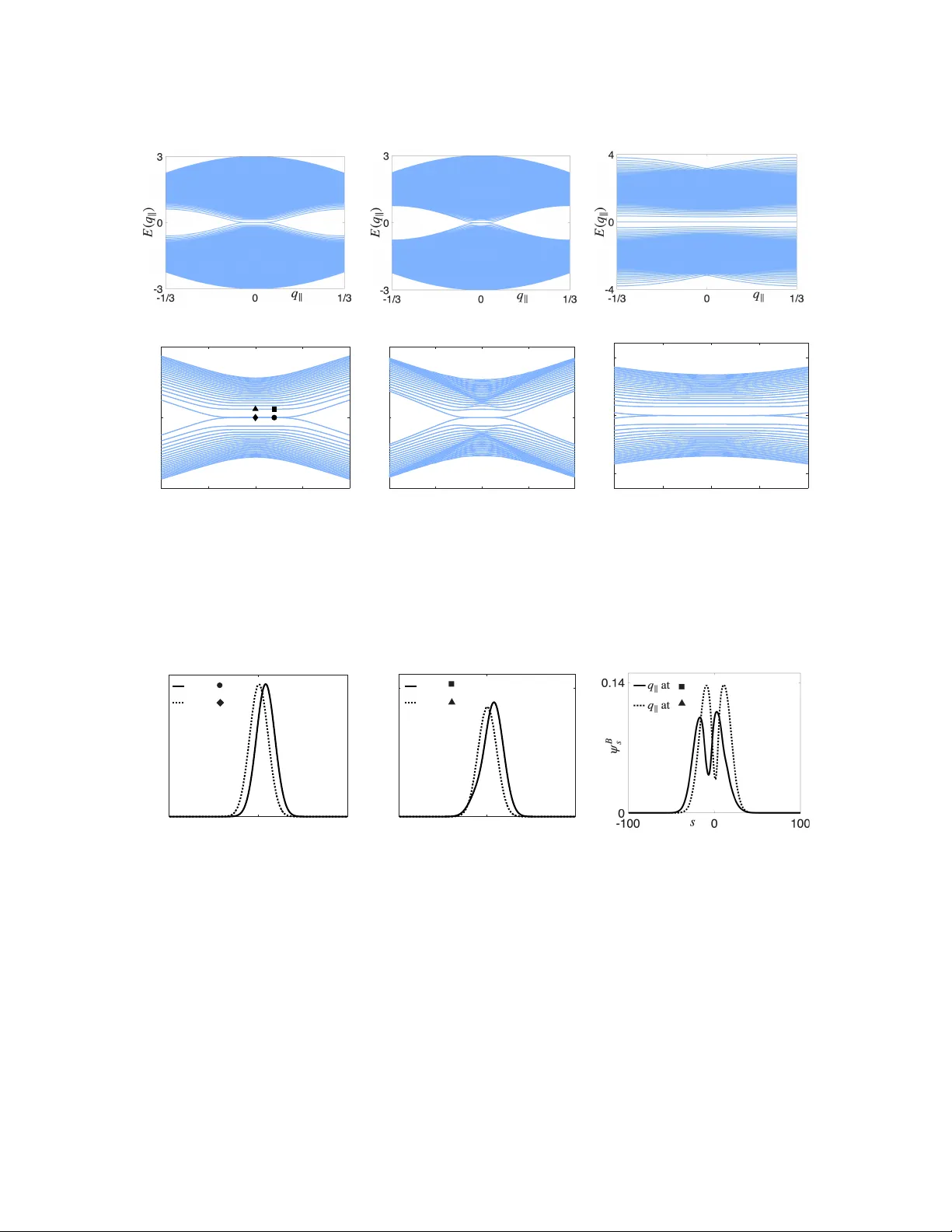
P seudo-magnetism in a strained discre te honeycomb lattice Xuenan Li * and Michael I. W einstein † March 31, 2026 Abstract Slowly varying nonuniform str ains of non-magnetic wave propagating media with honeycomb symmetry i nduce an effective- or pseudo- m agn etic ﬁeld, a phenomenon observed ﬁrst in graphene [ 4 ], and later in pho tonic crystals, e.g. [ 2 , 3 , 16 ] and oth er physical settings. Starting with a discrete nearest-neighbor tight-binding model of a non-uniformly s t r ained honeycomb medium, we derive the continuum effective magnetic Dirac Hamiltonian governing the envelope dynamics of wa v e packets, which are spectrally localized near a Dirac point (conical band degeneracy) of the unpertur be d hon- eycomb. F or unidirectional deformations of bounded gradient, which preser ve translation invariance along the “ar mchair” direction, w e prove the exi s t e nce of time-harmonic states which are plane-wave like (pseudo-periodic) along the armchair direction and exponentially localized transvers e to it. W e also obtain the leading order multi-scale structure of such modes for small de for mation gr adients. Their transverse localization are dete rmined by the e igenstates of a one dimensional effective Dir ac Hamiltonian. Our ri gor ou s r esults apply to deformations w hich i nduce an approximate perpendicu- lar constant pseudo-magnetic ﬁeld (Landau gauge ), and yield states with nearly ﬂat band (La ndau level) spectru m and hence ver y high density of states. In contrast, the analogous deformation which preserves translations in the zigzag direction induces no su ch localization. Corroborating numerical simulations for the diffe rent deformation types are prese nted. Contents 1 Introduction 3 1.1 Tig ht-binding mode l for a slowly varying deformation of th e honeycomb . . . . . . . . . 4 1.2 Summary of results . . . . . . . . . . . . . . . . . . . . . . . . . . . . . . . . . . . . . . . 6 1.3 R elated wor k . . . . . . . . . . . . . . . . . . . . . . . . . . . . . . . . . . . . . . . . . . 8 1.4 Future directions . . . . . . . . . . . . . . . . . . . . . . . . . . . . . . . . . . . . . . . . 9 1.5 Outline of the art icle . . . . . . . . . . . . . . . . . . . . . . . . . . . . . . . . . . . . . . 9 1.6 Notation and conventions . . . . . . . . . . . . . . . . . . . . . . . . . . . . . . . . . . . 10 * Department of Appl i ed Physics and Appli e d Mathematics, Columbia Univ ersity , xl3383@c olumbia.edu † Department of Applie d Physics a nd Applied Mathematics , and Dep artment o f Mathematics, Co l umbia Uni versity , miw2103@columb ia.edu 1 2 Ti ght-binding model on t h e honey comb lattice and Dirac points 10 2.1 T riangular lattice . . . . . . . . . . . . . . . . . . . . . . . . . . . . . . . . . . . . . . . . 11 2.2 Honeycomb lattice . . . . . . . . . . . . . . . . . . . . . . . . . . . . . . . . . . . . . . . 11 2.3 Tig ht-binding mode l on H . . . . . . . . . . . . . . . . . . . . . . . . . . . . . . . . . . . 12 2.4 Band structure of H 0 . . . . . . . . . . . . . . . . . . . . . . . . . . . . . . . . . . . . . . 13 3 Slow st rain induces an effective 2D Dirac magnetic Hamiltonian 13 3.1 Tig ht binding Hamiltonian for a slowly-strained discrete hone yco mb . . . . . . . . . . . 14 3.2 A formal discrete multiple scale ex pansion . . . . . . . . . . . . . . . . . . . . . . . . . . 16 3.3 H eff , the e f fective Hamiltonian, is a magnetic Dirac op e rator . . . . . . . . . . . . . . . . 18 4 Unidirectional deformations and th e l 2 k k -eigenvalue problem 19 4.1 Unidirectional deformations with b o unded gradients . . . . . . . . . . . . . . . . . . . . 23 5 Main th eorem: Eigenpairs of th e effect iv e magnetic Dirac operator se e d localized states 25 5.1 Our main theor em . . . . . . . . . . . . . . . . . . . . . . . . . . . . . . . . . . . . . . . 26 6 Corroboration of Theorem 5.1 via numerical simulations 28 7 Proof of Th eorem 5.1 33 7.1 Step 1: Equation for the corrector , η , and its DFT . . . . . . . . . . . . . . . . . . . . . . 33 7.2 Step 2: Decomposition of the corrector , η into “near”- and “far” quasi-momentum components 35 7.3 Step 3: solving the f ar -momentum equation . . . . . . . . . . . . . . . . . . . . . . . . . 37 7.4 The inverse oper at or of D − E 1 . . . . . . . . . . . . . . . . . . . . . . . . . . . . . . . . 40 7.5 Step 4: solving e η near and µ ( δ ) by Lyapunov-Schmidt reduction . . . . . . . . . . . . . . . 42 8 Summary and conc lusion 47 Appendix 47 A Quadratic defor mat ions with AC and ZZ or ientations . . . . . . . . . . . . . . . . . . . . 47 B Discrete F ourier transfor m and P oisson summation formula . . . . . . . . . . . . . . . . 51 C A review of classical results in exponential dichot omy th eory . . . . . . . . . . . . . . . . 53 D Numerical scheme and numerical artifacts . . . . . . . . . . . . . . . . . . . . . . . . . . 57 E Derivation of the 2D effect ive envelope e quations . . . . . . . . . . . . . . . . . . . . . . 59 F Derivation of the 1D effect ive envelope e quations . . . . . . . . . . . . . . . . . . . . . . 62 G The equation f or e η ( k ) , the corrector . . . . . . . . . . . . . . . . . . . . . . . . . . . . . . 64 H The derivation fo r t he near-momentum equation b β near . . . . . . . . . . . . . . . . . . . 69 S1 A gene ral cho ic e of hopping c oefﬁcients 75 S2 The unitary eq uivalence betwee n H eff and D A 76 S3 Pro o f of L emma 4.3 77 2 S4 Some useful calculations and bounds 84 1 Introduction Graphene and its synthetic variants are spatially periodic two-dimensional media, whose material properties h ave the symmetries of a honeycomb tiling of R 2 . W ave propagation in these media is governed b y wave equations, continuum ( Schrödinger , M axwell,. . . ) or discrete , wh ich are invariant under these symmetries. Central to the remarkable pr o perties of hone yco mb media is the presence of Dirac points . These are energy/quasi-momentum pairs at which two consecutive (Floquet-Bloch) dispersion surfaces touch conically . W ave p acket initial conditions which are spect rally localized to a size δ neighborhood of a D irac p oint, give rise to a time-evolving wave packet whose envelope, on a time scale δ − 2+ ǫ , is governed by a 2D effective Dirac e quation. Thus, such quasiparticle states evo lve as though they are massless relativistic particles. A mathematically rigorous analysis in the conte xt of the underlying continuum Schrödinger equation with a honeycomb lattice potential was given in [ 14 ]; see also [ 20 ]. Shortly after the graphene’s discover y , it was ob served that slowly varying non-uniform def orma- tions of graphene give rise t o a pseudo-magnetic effect [ 4 ]. Based on a tight-binding (discret e) models, it was de duced that the wave packet envelope satisﬁes an effect ive magnetic D irac equation. Thus, in t he absence of any ext e rnal magnetic ﬁeld, quasi-particles modeled by wave p ackets move as though they are charged particles in a magnetic ﬁ eld. Further , when the defo r mation is cho sen to induce an effec- tive magnetic ﬁe ld which is constant and perpendicular to the two-dimensional p lane of t he material (schematic of Figure 1 (c)), the spect rum of waves consists of highly degenerate states, which arise as “Landau levels” in eff ective magnetic Dirac Hamiltonian (schematic of Figure 1 (d)). The signiﬁcance of Landau level and other “ﬂat band” spectra is that it can be leveraged to enhance stro ng interac- tions and nonlinear eff ects. The rich phenomena associated with Landau Levels in co ndensed matter physics, have inspired investigations, in diver se physical settings, to re alize the pseudo-magnetic effect. A particular direction concerns p h otonics and, in par ticular , photonic crystals. While the t ight- binding models explain pseudo-magnetism in condensed matter se t tings, this approximation does not valid in photo nic settings. In [ 16 ] the effective dynamics was studied in the setting of general contin- uum wave equations, and where both magnetic and effective electric potentials arise in the e ffective Dirac Hamiltonian. Expe rimental o b servation of photonic Landau levels in 3D photonic crystal was observed in [ 2 , 3 ]. Further , an ext e nsion of the 2D theor y to 3D gives an excellent agreement with experiments [ 3 ]. Our goal in th is article, is to p resent a r igorous de rivation of wave localization due to a non- uniform defor mat ion induced pseudo-magnetic ﬁeld. W e study th is question in the context of class of tight-binding with general slowly varying hopping coef ﬁcients. Our results, state d more p r ecisely below , apply to unidirectional def ormations with b ounded gradients. In this set t ing we p rove the validity of the magnetic Dirac ope r ator , exp lore ( Landau gauge type) def ormations which give rise to approximate Landau level spectra, as well as de f ormations that pro duce other be haviors. In particular , we prove th at the localized states of an effective asymptotic Dirac ope rator , seed localized states of the 3 underlying tight-binding Hamiltonian. Finally , we provide numerical co rroboration of our results. The family of tight-binding models studied in this article cap t ures the essential physical be havior in t he condensed matter setting; see e.g. [ 17 , 23 ]. As discussed in [ 16 ], tight-binding is not the appropriate app r oximation in, for example, photonic crystals. W e remark h owever t h at our discrete model captures the main prope r ties of waves which ar e spectrally localized near the Dirac point for both Schrödinger and Helmholtz equations, and is more amenable to full rigorous analysis since one need no t control arb itrarily high energies; indeed the spect r um of the tight-binding Hamiltonian is bounded. Our plan is to e x tend the prese nt wor k to continuum mo d e ls in a future wo r k. Before summarizing our main results, we next present a more precise f ormulation of the tight- binding model. (a) (b) (c) k k E - √ 3 ∆ E - √ 2 ∆ E - ∆ E 0 ∆ E √ 2 ∆ E √ 3 ∆ E n = 2 n = 3 n = 1 n = 0 n = − 1 n = − 2 n = − 3 . . . . . . (d) Figure 1: The undeformed and def ormed honeycomb and the ir band str uctures: (a) the undeformed honeycomb with the unit cell highlighted by shading; (b) the band structure of the tight-binding Hamiltonian H 0 for the undef o rmed honeycomb with Dirac points occurring at the intersect ion of the two dispersion surfaces, at the six ver tices of the Brillouin zo ne B ; (c) th e deformed honeycomb with a slowly-varying quadratic de formation u ( δ X ) = (0 , δ 2 X 2 1 ) T ; (d) Landau levels generated by the effect of strain in ( c) o n the spect rum. 1.1 T ight-bin ding model for a slowly varying deformation of t he honeycomb Let A m,n , B m,n denote the vertices of the h oneycomb lattice; see Figure 1 a and the more detailed discussion in Section 2 . Each A − site has 3 nearest neighbor B − sites and each B − site h as 3 nearest neighbor A − sites. The positions o f the three nearest B − sites to A m,n are B m + m ν ,n + n ν , ν = 1 , 2 , 3 and the thr ee nearest A − sites to B m,n are A m − m ν ,n − n ν with ν = 1 , 2 , 3 . W e take | A m,n − B m,n | = 1 , fo r all ( m, n ) ∈ Z 2 , to be t h e lattice spacing b etween nearest neighbors. 4 Introduce a smooth displacement ﬁe ld x 7→ u ( x ) . F or δ > 0 and small we de ﬁne a slowly-strained honeycomb lattice whose vertices are at the positions e A m,n = A m,n + u ( δ A m,n ) , ‹ B m,n = B m,n + u ( δ B m,n ) . The undistort ed honeycomb lattice, δ = 0 , with a choice of period lattice vectors and per iod ce ll, is displayed in Figure 1 a and an example of a weakly and non-uniformly (quadratically) strained lattice is displayed in Figure 1 b. A wave function, ψ , is an assignment of a complex amplitude to each site. W e group the amplitudes by cell and write: ψ = ( ψ m,n ) ( m,n ) ∈ Z 2 , where ψ m,n = ψ A m,n ψ B m,n ! ∈ C 2 . The strength of inter action between t h e amplitude at a given site and the amplitudes at t h e thr ee nearest neighbor sites, depends on the distance between nearest neighbor sites. F or two neare st neigh- bor sites e A and ‹ B , we deﬁne: t ( e A, ‹ B ) = h ( | e A − ‹ B | ) = t ( ‹ B , e A ) , (  .  ) where h is a speciﬁed smooth scalar function. W e set t 0 = h (1) and t 1 = h ′ (1) . The nearest neighbor tight-binding model, H δ (undeformed, δ = 0 and defor med, δ > 0 ) acts on ψ ∈ l 2 ( Z 2 ; C ) is deﬁ ne d by: H δ ψ = ( H δ ψ ) A m,n ( H δ ψ ) B m,n ! = P 3 ν =1 t ( e A m,n , ‹ B m + m ν ,n + n ν ) ψ B m + m ν ,n + n ν P 3 ν =1 t ( ‹ B m,n , e A m − m ν ,n − n ν ) ψ A m − m ν ,n − n ν ! . (  .  ) F or δ = 0 , e A m,n = A m,n and ‹ B m,n = B m,n . Hence, for t he undeformed lattice, t ( A m,n , B m,n ) = h (1) ; all h o pping coefﬁ cients of the undeformed Hamiltonian H 0 are e qual. This yields H 0 , the tight- binding mod e l for the undeformed honeycomb with uniform hopping coefﬁcient t 0 . The Hamiltonian H 0 has a band structure, deducible via the two-dimensional discret e F ourier transfo r m, consisting of two band dispersion surf aces which meet co nically at high symmetry quasimomenta, the ver tices o f the hexagonal Brillouin z o ne; see Figure 1 (b). F or the de f ormed tight-binding Hamiltonian ( 0 < δ ≪ 1 ), as hopp ing coefﬁcients in (  .  ) we re- place t ( e A m,n , ‹ B m + m ν ,n + n ν ) and t ( ‹ B m,n , e A m − m ν ,n − n ν ) in (  .  ) b y the ir O ( δ ) -correct ions. F o r e xample, the in-cell hopping coefﬁ cients are obtained b y expansion o f δ 7→ h ( | e A m,n − ‹ B m,n | ) t h rough order δ and dropping ter ms of order O ( δ 2 ) : t ( e A m,n , ‹ B m,n ) ≡ t 0 + δ t 1 e T 1 ∇ X u ( δ A m,n ) e 1 . Analogous exp ressions for the ho ppings ar e displayed be low in (  .  ). The resulting Hamiltonian, H δ , varies on two spatial scales: the O (1) length scale o f the lattice, and th e long O ( δ − 1 ) length scale of the lattice defor m at ions. 5 1.2 Summary of results • Using t he multiple scale structure of our Hamiltonian, we ﬁrst co nstr uct formal asymptotic ex - pansion of eigenpairs ( ψ δ , E δ ) eigenvalue problems H δ ψ = E ψ subject to appropriate homoge- neous boundary conditions at ∞ . Eigenmodes have a two-scale wave p acke t str ucture: ψ δ m,n = e i K · x Φ ( X ; δ )    X = δ ( m v 1 + n v 2 ) , where ( m, n ) ∈ Z 2 , (  .  ) and are constr ucte d as a fo rmal series Φ ( X ; δ ) = P j ≥ 0 δ j Φ j ( X ) . If, for example, X 7→ Φ ( X ; δ ) decays sufﬁciently rapidly at | X | 7→ ∞ , then the discrete F ourier transform of (  .  ) is spe ctrally concentrated in a δ − width neighborhood to t he h igh symmetry quasi-momentum K . At leading order in δ , we ﬁnd that ψ δ m,n ≈ e i K · x Φ 0 ( X )    X = δ ( m v 1 + n v 2 ) and E δ ≈ δ E 1 where – up to a unitary change of variables – ( Φ 0 ( X ) , E 1 ) is an eigenpair , of an ef fective magnetic Dirac operat or: D A =  − i∂ X 1 − A 1 ( X 1 , X 2 )  σ 1 +  − i∂ X 2 − A 2 ( X 1 , X 2 )  σ 2 , (  .  ) with effect ive magnetic pote nt ial A eff = ( A 1 , A 2 ) , given explicitly in terms of the defo rmation u ( X ) . • Motivated by t he case of Landau gauge for a constant p erpendicular magnetic ﬁ eld, we focus on unidirectional defo rmations u = (0 , d ( X 1 )) T , for which the deformed structure are translation invariant in the v 2 (vertical) direction. Hence, t he spectral theory of H δ acting in the space l 2 ( Z 2 ; C 2 ) is r educible t o a family of q k − pseudo-periodic spect ral pr oblems, parameterized by q k ∈ [ − π , π ) . W e ar e particularly inter e sted in t h e discret e eigenvalues. The se are nontrivial solutions of the form ψ m,n = e inq k Ψ m ( q k ) , where  H δ ( q k ) Ψ  m = E ( q k ) Ψ m , Ψ ( q k ) = ( Ψ m ) m ∈ Z ∈ l 2 ( Z ; C 2 ) . (  .  ) Given a continuous family of solutions q k ∈ I 7→ Ψ ( q k ) , for q k varying over a subinterval I ⊂ [ − π , π ) , we may form continuous superposions to produce stat es which have full spatial localization over the lattice; equivalently , such states are in l 2 ( Z 2 ; C 2 ) . F or the q k − p seudo-periodic eigenvalue problem (  .  ) with q k = δ k k , our multiple scale expan- sion yields approximate eigenpairs ( Ψ δ ( k k ) , E δ ( k k )) where Ψ δ ( k k ) is k k − pseudo-periodic in th e v 2 direction and spatially localized in tr ansverse direct ions. Up to coordinate change, the mode proﬁle has the structure ψ approx m,n ( k k ) = δ 1 2 e i K · x e i k k 2 π X · a 2 Ψ # 0 Å X · a 1 | a 1 | ; k k ã     x = C m,n X = δ C m,n (  .  a) 6 E approx ( k k ) = δ E 1 ( k k ) , | k k | . 1 , (  .  b) where  Ψ # 0 ( X 1 ; k k ) , E 1 ( k k )  is an L 2 X 1 ( R ) − eigenpair o f a o ne-dimensional Dirac operator aris- ing from (  .  ): D ( k k ) := 3 2 h − i∂ X 1 σ 1 + κ ( X 1 ; k k ) σ 2 i , κ ( X 1 ; k k ) = k k 3 − t 1 2 d ′ ( X 1 ) ; (  .  ) see also (  .  ). F or k k in an interval about 0 , the L 2 ( R ) spectrum of D ( k k ) consists of a continuous part, with a spectral gap containing an odd number of eigenvalues. T he eigenvalue curve k k 7→ E 0 ( k k ) , for which E 0 (0) = 0 , is “topologically pro tected”; it cannot be removed by a spatially localized pert urbation of κ . • Introduce l 2 k k , the space of all ψ = ( ψ m,n ) m,n ∈ Z which satisfy: ψ δ m,n +1 = e i ( δk k ) ψ δ m,n , (pseudo-periodicity) (  .  a) m ∈ Z 7− → ψ m,n ∈ l 2 m ( Z ) (transverse localization) . (  .  b) Our main t heorem is Th eorem 5.1 , which states that for 0 < δ < δ 0 sufﬁciently small and | k k | . 1 the following ho lds: any eigenpair of D ( k k ) gives rise to an eigenpair of the l 2 k k -eigenvalue problem ( H δ ψ ) m,n = E δ ψ δ m,n , ψ ∈ l 2 k k (  .  ) Moreover , we have the following bound for the correct o rs: sup n ∈ Z    ψ δ m,n ( k k ) − ψ approx m,n ( k k )    l 2 m ( Z ; C 2 ) . δ, (  .  a) | E δ ( k k ) − δ E approx 1 ( k k ) | . δ 2 . (  .  b) Here, the leading ap p roximations to ( ψ δ , E δ ) are displayed in (  .  ). • W e p e rform numerical simulations for two classes of deformat ions of the under lying honeycomb structure: (1) armchair o r iented deformat ions (see e .g. Figure 10a ) and zigzag oriented de for- mations (see e.g. F igure 10c ). F or these conﬁgurations, we investigate the spectral char act eristics of the resulting Hamiltonian in a neighborhood of the Dirac point. F or th e quadratic defor mation along the AC orientation, which is o ur main fo cus, the numerical eigenvalues of the Hamiltonian H δ in (  .  ) are near ly independent of the quasi-momentum q k near the D irac point q k = 0 (see Figure 2 (b)), indicating the pre sence of Landau levels. The eigenmodes are localized in the bulk, as shown in Figures 2 (b-c). F or the quadratic deformation along t he ZZ orientation, th e Dirac point is not opened into ﬂat bands; the cr ossing pe r sists from one side (see Figures 9 (b) and (d)). This agrees with the effective Hamiltonian b eing p urely continuous spectrum near the Dirac point, so no discrete localized modes e me rge. 7 q k -0.15 -0.07 0 0.07 0.15 E ( q k ) -0.5 0 0.5 (a) q k -0.1 -0.05 0 0.05 0.1 E δ ( q k ) -1 0 1 (b) s -100 0 100 ψ A s 0 0.25 q k at q k at (c) s -100 0 100 ψ A s 0 0.18 q k at q k at (d) Figure 2: (a) Conical (D irac) point occurs at q k = 0 ; (b) Nonuniform deformation u = (0 , X 2 1 ) T (approximation to Landau gauge vecto r p o tential) creates a b ulk gap with quite ﬂat (Landau level like) localized mode eigenvalue curve s E δ ( q k ) in t he gap; (c) Localized eigenstates corre sponding to the diamond and circle in ( b); ( d) Localized eigenstates corresponding to t he triangle and square in (b). 1.3 R elated work In [ 26 ] it is shown that the d ynamics of a class of wave-packets of deformed cont inuum honeycomb media is gover ne d , on large but ﬁnite time scales, by the effective magnetic Dirac op e rator , de rived in [ 16 ]; see also [ 3 ]. The approach taken is similar to that in [ 14 ] for the dynamics of wavepackets in undistorted honeycomb str uctur e s. T h e article [ 1 ] de velops, via pseudo -differential calculus, a frame- work for studying th e large (ﬁ nite) time dynamics in discrete systems with slowly varying hopping coefﬁcients. Spatial localization in defo rmed ho neycomb structure s, as we show ar ises from t he eigenstates of an asympto tic (effective) Dirac Hamiltonian with a domain wall potential. Analogous localization phenomena arise in the study of edge states of honeycomb or o ther media with band degeneracies, when p erturbed along a line defect o r “edge”; see e.g. [ 5 , 7 , 8 , 9 , 11 , 20 ]. 8 1.4 F uture directions 1. Our current re sults are based on a tight-binding mode l with slowly varying coefﬁcients. A f uture direction is to generalize this setting to a continuum the o ry that captures not only the low-energy regime but also higher-energy bands. 2. W e show point spectr um o f an effective Dir ac operator give rise to l 2 k k -eigenstates of the under ly- ing deformed tight-binding Hamiltonian, H δ . Do all such localized states of the discrete operator arise in this manner? W e believe t his to be the case, and that a quasi-mode approach, like that used in [ 7 ], would be app licable. 3. In th e pr e sent tight-binding model, only nearest-neighbor couplings are included, and the re- sulting e ffective Dirac Hamiltonian co nt ains only a pseudo-magnetic po t ential. The addition of next-nearest-neighbor couplings (see e.g. the Haldane model in [ 18 ]), would give rise to effec- tive Dirac Hamiltonians with a pseudo-electric potential as well (see e.g. [ 16 ]). 4. Spa tially co mpact deformatio ns and sc a ttering resonances : I n practice, strain ﬁelds are applied over a ﬁnite re gion (due to sample size and f abrication limits). Therefor e, it is natural to consider the case of strain which is conﬁned to a large compact set. In this case, we do not expe ct the effective Dirac Hamiltonian to suppor t localized states. W e do however e xpect scattering resonances (see e.g. [ 10 , 24 ]) which capture th e effect of slow ener gy leakage out of the region where the structure is def o rmed. An analytical and numerical investigation would be of great interest. 5. T riaxial deformati on: A second deformation, unlike the unidirectional quadratic d e formation u ( X 1 , X 2 ) = (0 , X 2 1 ) T , which also generate s a constant pseudo-magnetic ﬁeld is the triaxial deformation [ 17 , 23 ], f or deﬁned by u ( X 1 , X 2 ) = (2 X 1 X 2 , X 2 1 − X 2 2 ) T . This deformation is rotational symmetric and gives rise to th e effective magnetic potential A eff = 2 t 1 ( − X 2 , X 1 ) in (  .  ). This is the well-known symm et ric gauge magnetic p otential fo r a constand pe rpendicular magnetic ﬁeld. Th e spectr al properties of the effective Hamiltonian D A in (  .  ) for the symmet- ric gauge have been extensively studied; the spectrum of D A consists is discrete spectr um and consists of eigenvalues of inﬁnite multiplicity (Landau levels). W e believe our strategy f or uni- directional deformations can be exte nded to bounded gradient regularizations of the symmetric gauge. 1.5 Outline of the article The re mainder of t his article is organized as follows. Section 2 re views the discrete honeycomb lattice and the undeforme d t ight-binding Hamiltonian. Sect ion 3 intr oduces the slowly str ained tight-binding model and derives the effective magnetic Dirac description via a f o rmal discrete multiscale expansion. In Section 4 , we introduce unidirectional deform at ions, which pre serve ver tical pe r iodicity , and reduce the eigenvalue prob lem to a one-dimensional one. I n Section 5 , we state our main Th eorem, Th e orem 5.1 , and o utline the sketch of the proof. I n Section 6 , we present numerical results for quadrat ic 9 deformations and their linear regularizations. W e pr ove Theor e m 5.1 in det ail in Section 7 . W e conclude our paper with a brief summary and some future directions in Section 8 . 1.6 Notation and conventions (1) ¯ z denotes the comp lex conjugate of z ∈ C . (2) x . y means that there exists a constant C > 0 such that x ≤ C y . (3) l 2 ( Z ; C 2 ) = { ( x n ) n ∈ Z | x n ∈ C 2 and P n ∈ Z | x n | 2 < ∞} and l 2 ( Z 2 ; C 2 ) = { ( x m,n ) m,n ∈ Z | x m,n ∈ C 2 and P m,n ∈ Z | x m,n | 2 < ∞} . (4) The Schwartz space S = S ( R , C ) : f ( x ) ∈ S ( R ) if f ∈ C ∞ ( R ) and for every pair of multi-indices α, β ∈ N n 0 , we have sup x ∈ R | x α ∂ β f ( x ) | < ∞ , where x α := x α 1 1 · · · x α n n and ∂ β := ∂ β 1 x 1 · · · ∂ β n x n . (5) Hilbert space H s ( R ) = H s ( R , C ) = { f : R 7→ C | R R (1 + | k | 2 ) s | b f ( k ) | 2 dk < ∞} . (6) L 2 , 1 ( R ) = n b f ( ξ )   R R (1 + | ξ | 2 ) | b f ( ξ ) | 2 dξ < ∞ o and the nor m in L 2 , 1 ( R ) space is deﬁned as k b f k 2 L 2 , 1 ( R ) = Z R (1 + | ξ | 2 ) | b f ( ξ ) | 2 dξ . (  .  ) By Plancherel, the condition b f ∈ L 2 , 1 ( R ) is equivalent to f ∈ H 1 ( R ) . (7) The space of C ∞ b ( R ) consists of functions on R whose derivatives of all orders are bounded , i.e. C ∞ b ( R ) = n f ∈ L ∞ ( R )    f ( k ) ∈ L ∞ ( R ) , for all k ≥ 1 o . (  .  ) (8) P auli matr ices σ 1 , σ 2 , σ 3 are σ 1 = 0 1 1 0 ! , σ 2 = 0 − i i 0 ! , σ 3 = 1 0 0 − 1 ! . (  .  ) Acknowledgement This work was supporte d in part by NSF grants: DMS1908657, DMS-1937254 and DMS-2510769, and Simons F oundation Math+X Investigator A ward #376319. P art of th is r e- search was carried out during the 2023-24 academic year , when MIW was a Visi ting Memb er in the School of Mathemat ics, Institute of Advanced St udy , Princeton, suppo r ted by the Charles Simonyi Endowment, and a V isiting F ellow in the D epartment of Mathematics at Princeton University . 2 Tight-bin ding model on the honey co m b lattice and Dirac p o ints In this section we discuss the discrete honeyco mb lattice and the associated tight-binding mode l of bulk (undefo rmed) graphene. This op erator is well-known to have Dirac points; its two dispersion surfaces (bands) which to uch conically at the ve r tices of the Brillouin zone; see e.g. [ 4 , 12 , 25 ]. 10 2.1 T riangular lattice The equilateral tr iangular lattice is the set Λ = Z v 1 ⊕ Z v 2 of all integer linear comb inations of the lattice vectors v 1 =  √ 3 2 , − 3 2  T , v 2 =  0 , 3  T . (  .  ) Introduce the dual lattice basis { a 1 , a 2 } , a 1 = 4 π √ 3 (1 , 0) T , a 2 = 4 π 3 Ç √ 3 2 , 1 2 å T , v i · a j = 2 π δ ij , (  .  ) and the dual lattice Λ ∗ = Z a 1 + Z a 2 ; see F igure 3a and Figure 3c . The Brillouin zone B is a choice of fundamental domain f o r R 2 / Λ ∗ , here chosen to be Brillouin zone is the hexagon shown in Figure 3c . with high-symmetry corner p oints K and K ′ (marked by solid and op e n dot s, respectively , in Figure 3c ). The vertices of the B are the points: K = 1 3 a 1 , K ′ = − 1 3 a 1 + a 2 , (  .  ) and their rotations by 2 π / 3 with r espect to the cente r of the hexagon. 2.2 Honeyco mb lattice The honeycomb lattice is the union of two inte rpenetrating t r iangular lattices, with base points at A 0 , 0 := (0 , 0) T and and B 0 , 0 := ( − √ 3 / 2 , − 1 / 2) T : H = Λ A ∪ Λ B , where Λ A = A 0 , 0 + Λ and Λ B = B 0 , 0 + Λ . (  .  ) The plane, R 2 , can be tiled b y parallelograms, generat ed by v 1 and v 2 and such t h at each of the se parallelograms contains two sites or nodes of H , an A − no d e and a B − node. The p arallelograms are indexed by pairs ( m, n ) ∈ Z 2 , and the nodes of H in the ( m, n ) ce ll are: A m,n = A 0 , 0 + m v 1 + n v 2 and B m,n = B 0 , 0 + m v 1 + n v 2 . (  .  ) The honeycomb lattice, H , is a bipar t ite lattice; each A − no d e has three nearest neighbhor B − nodes and each B − node has thr e e nearest neighbor A − nodes. Starting with an A − or B − node), the nearest neighbor A − and B − nod e s are obt ained by displacement by ± e ν , ν = 1 , 2 , 3 , where e 1 =  √ 3 2 , 1 2  T , e 2 =  − √ 3 2 , 1 2  T , e 3 =  0 , − 1  T . (  .  ) Hence, for ν = 1 , 2 , 3 , the nearest B − nodes to A m,n are B m + m ν ,n + n ν , and (  .  a) the nearest A − node s to B m,n are A m − m ν ,n − n ν , where (  .  b) 11 ( m 1 , n 1 ) = (0 , 0) , ( m 2 , n 2 ) = (2 , 1) , and ( m 3 , n 3 ) = (1 , 1) . (  .  c) (a) e 2 B m,n e 3 A m − 1 ,n − 1 A m,n B m +1 ,n +1 B m +2 ,n +1 A m − 2 ,n − 1 e 1 (b) K = a 1 / 3 B a 1 K ′ = − a 1 / 3 + a 2 a 2 (c) Figure 3: (a) The honeycomb lattice, Z v 1 + Z v 2 , containing t wo nodes, A in red and B in blue, per unit cell. R 2 is the union o f cells (parallelograms), each containing two nodes (circled pair of dots), labeled with Z 2 indices. Dark-shaded parallelogram is the ( m, n ) -cell; adjacent lighter-shaded regions are translations by ± v 1 or ± v 2 . (b) nearest neighbors of A m,n and B m,n , bond direct ion vect ors e i ( i = 1 , 2 , 3 ); (c) Hexagonal Brillouin zo ne B with high symmet ry quasimomenta K , K ′ , at the ver tices of B . Dual lattice vectors a 1 , a 2 , such t h at a l · v j = 2 π δ lj . 2.3 T ight-bin ding model on H A “wave function” is an assignment of a complex-valued amplitude to each node of H . I t is convenient to organize these as complex amplitude p airs, corresponding to each cell: ψ = ( ψ m,n ) m,n ∈ Z , ψ m,n = ψ A m,n ψ B m,n ! ∈ C 2 . (  .  ) W e take as our Hilbert space l 2 ( H ) := l 2 ( Z 2 ; C 2 ) with norm deﬁned by k ψ k 2 = X ( m,n ) ∈ Z 2 k ψ m,n k 2 C 2 < ∞ . (  .  ) 12 The nearest neighbor tight-binding Hamiltonian H 0 on the honeycomb lattice (the superscript 0 refers to the undefor med h oneycomb), is the nearest neighbor operat or: ( H 0 ψ ) m,n := ( H 0 ψ ) A m,n ( H 0 ψ ) B m,n ! = P 3 ν =1 ψ B m + m ν ,n + n ν P 3 ν =1 ψ A m − m ν ,n − n ν ! . (  .  ) H 0 is a self-adjoint and bounded linear operator on l 2 ( Z 2 ; C 2 ) . 2.4 Band st r u cture of H 0 W e study the spe ct rum of H 0 via the 2D discrete F ourier transform (DF T ); see Appendix B . F or ψ = ( ψ m,n ) m,n ∈ Z ∈ l 2 ( H ) , we deﬁne ‹ ψ ( k ) = X m,n ∈ Z e − i k · ( m v 1 + n v 2 ) ψ m,n . (  .  ) The mapping k 7→ ‹ ψ ( k ) is in L 2 ( R 2 / Λ ∗ ) with period ce ll B ; see F igure 3c . T he band structure of H 0 is given by the two eigenpairs (band dispersion curves and Floquet-Bloch modes) of o f t he 2 × 2 matrix: ‹ H 0 ( k ) = 3 X ν =1 0 e i k · w ν e − i k · w ν 0 ! , k ∈ B . (  .  ) Here w ν = m ν v 1 + n ν v 2 = e 1 − e ν : w 1 = (0 , 0) T , w 2 = e 1 − e 2 = ( √ 3 , 0) T , w 3 = e 1 − e 3 = Ç √ 3 2 , 3 2 å T . (  .  ) The band dispersion f unctions are given by: E ± ( k ) = ±      3 X ν =1 e i k · w ν      . (  .  ) The two dispersion surfaces touch the over t he vert ices o f B ; for k ∈ B , E + ( k ) = 0 = E − ( k ) if and only if k = K , K ′ or one of their rotat ions by 2 π / 3 ; see (  .  ) and F igure 1b . The local character of the touching dispersion surfaces at these high symmetry quasi-momenta is conical and the corr e sponding energy / quasi-momentum pairs are called Dirac points . The spectrum of H 0 , acting in l 2 ( H ) , is continuous and equal to the interval [ − 3 , 3] . 3 Slow strain induces an ef f ective 2D Dirac m agnetic Hamiltonian W e now introduce a tight-binding Hamiltonian for a slowly strained honeycomb lattice and propo se a two-scale wave-packet ansatz for the associated eigenvalue prob lem. W e t hen present a formal dis- crete multiscale expansion of th e resulting two-scale eigenstates, yielding an effect ive two-dimensional magnetic Dirac equation. 13 3.1 T ight binding Hamiltonian for a slowly-strained discrete honeyc omb W e consider a slowly-strained discrete ho neycomb, where the undeformed nodes, A m,n , B m,n are mapped, under the smooth and slowly-varying displacement X 7→ u ( X ) = u ( X 1 , X 2 ) to: e A m,n = A m,n + u ( δ A m,n ) , ‹ B m,n = B m,n + u ( δ B m,n ) , 0 < δ ≪ 1 . (  .  ) W e now introduce the neare st neighbor tight-binding Hamiltonian H δ for the deformed honeycomb lattice. F or a wave function ψ = ( ψ m,n ) m,n ∈ Z ∈ ℓ 2 ( Z 2 ) , we have: ( H δ ψ ) m,n = ( H δ ψ ) A m,n ( H δ ψ ) B m,n ! = P 3 ν =1 t ( e A m,n , ‹ B m + m ν ,n + n ν ) ψ B m + m ν ,n + n ν P 3 ν =1 t ( ‹ B m,n , e A m − m ν ,n − n ν ) ψ A m − m ν ,n − n ν ! . (  .  ) Here, t ( ‹ X , ‹ Y ) is the hopp ing coefﬁcient between th e defor me d nodes ‹ X and ‹ Y , he re taken to be of t he form: t ( e A m,n , ‹ B m,n ) := h ( | e A m,n − ‹ B m,n | ) , (  .  ) where h : R + 7→ R is a smooth function such that: h (1) = 1 and h ′ (1) = t 1 . The parameter t 1 controls how the hopp ing coef ﬁcient d epends on the str ain: when t 1 > 0 , th e ho pping strength increases with strain, while for t 1 < 0 , it de cr eases. F or simplicity , rather than working with H δ in (  .  ), we seek a tight binding model which in- corporates only order δ corrections to H 0 . Since | A m,n − B m,n | = 1 , we ﬁ nd | e A m,n − ‹ B m,n | = | A m,n − B m,n + u ( δ A m,n ) − u ( δ B m,n ) | = 1 + O ( δ ) . Expanding t ( e A m,n , ‹ B m,n ) in (  .  ) f or small δ , we obtain (details in Appendix S1 ) t ( e A m,n , ‹ B m,n ) = 1 + δ t 1 e T 1 ∇ X u ( δ A m,n ) e 1 + O ( δ 2 ) , (  .  ) where e 1 = A m,n − B m,n is deﬁned in (  .  ) and ∇ X u ( X ) de notes t he 2 × 2 Jacobian matrix. T Note that since δ B m,n lies O ( δ ) -away f rom δ A m,n , an expression for the hopping coefﬁcient t ( e A m,n , ‹ B m,n ) , which is asymptotically equivalent to (  .  ) is the expression: t ( e A m,n , ‹ B m,n ) = 1 + δ t 1 e T 1 ∇ X u ( δ B m,n ) e 1 + O ( δ 2 ) . In exp anding the hopping coefﬁ cients through order δ , we’ll make t h e consistent choice of the A − point in each cell, as the r e ference po int about which we expand. Thus we set C m,n := A m,n = m v 1 + n v 2 = Ç √ 3 2 m, − 3 2 m + 3 n å T , (  .  ) This choice leads to a self-adjoint Hamiltonian is shown in Appe ndix S4 . Expansion of the hopp ing coefﬁcient t h rough ord er δ and dropping all terms of or d e r δ 2 and higher , we obt ain the f ollowing 14 hopping coefﬁcients: t ( e A m,n , ‹ B m ± m 1 ,n ± n 1 ) = t ( e A m,n , ‹ B m,n ) = 1 + δ t 1 e T 1 ∇ X u ( δ C m,n ) e 1 , (  .  a) t ( e A m,n , ‹ B m + m 2 ,n + n 2 ) = t ( e A m,n , ‹ B m +2 ,n +1 ) = 1 + δ t 1 e T 2 ∇ X u ( δ C m,n ) e 2 , (  .  b) t ( e A m,n , ‹ B m + m 3 ,n + n 3 ) = t ( e A m,n , ‹ B m +1 ,n +1 ) = 1 + δ t 1 e T 3 ∇ X u ( δ C m,n ) e 3 , (  .  c) t ( ‹ B m,n , e A m − m 2 ,n − n 2 ) = t ( ‹ B m,n , e A m − 2 ,n − 1 ) = 1 + δ t 1 e T 2 ∇ X u ( δ C m − m 2 ,n − n 2 ) e 2 , (  .  d) t ( ‹ B m,n , e A m − m 3 ,n − n 3 ) = t ( ‹ B m,n , e A m − 1 ,n − 1 ) = 1 + δ t 1 e T 3 ∇ X u ( δ C m − m 3 ,n − n 3 ) e 3 . (  .  e) Here, the scalar quantity e T i  ∇ X u ( δ C m,n )  e i with i = 1 , 2 , 3 represents the linear strain induced by u at the edge in the e i direction in the ( m, n ) -th cell. Our selection of hopping coefﬁcients in (  .  ) is consistent with th o se commo nly used in the physics literature (see Equation (172) in [ 4 ]). Let f ν ( X ) := e T ν  ∇ X u ( X )  e ν , ν = 1 , 2 , 3 . (  .  ) Explicitly , we h ave : f 1 ( X ) = e T 1 ( ∇ X u ) e 1 = 3 4 ∂ X 1 u 1 + √ 3 4 ( ∂ X 1 u 2 + ∂ X 2 u 1 ) + 1 4 ∂ X 2 u 2 , (  .  a) f 2 ( X ) = e T 2 ( ∇ X u ) e 2 = 3 4 ∂ X 1 u 1 − √ 3 4 ( ∂ X 1 u 2 + ∂ X 2 u 1 ) + 1 4 ∂ X 2 u 2 , (  .  b) f 3 ( X ) = e T 3 ( ∇ X u ) e 3 = ∂ X 2 u 2 . (  .  c) The deformed Hamiltonian H δ , an O ( δ ) pert ur b ation of H 0 , is given by: ( H δ ψ ) m,n = ( H δ ψ ) A m,n ( H δ ψ ) B m,n ! = Ñ P 3 ν =1  1 + δ t 1 f ν ( δ C m,n )  ψ B m + m ν ,n + n ν P 3 ν =1  1 + δ t 1 f ν ( δ C m − m ν ,n − n ν )  ψ A m − m ν ,n − n ν é , (  .  ) The operator H δ is formally self-adjoint in l 2 ( Z 2 ; C 2 ) ; see t h e Supplement ar y Material S4 . Our goal is to study eigenvalue problems for H δ : H δ ψ = E ψ (  .  ) subject to a suitable choice of self-adjoint boundary conditions; f or example: (a) ψ = ( ψ m,n ) m,n ∈ Z ∈ l 2 ( Z 2 ; C 2 ) , or (b) in the case wher e the deformation is invariant under with respect to v 2 (and thus f ν ( δ C m,n ) depends only on m ), we impose: m 7→ ψ m,n ∈ l 2 ( Z ; C 2 ) and ψ m,n +1 = e iq k ψ m,n , where q k ∈ [ − π , π ] is the parallel quasi-momentum related associated with this translation invariance of ( H δ ψ ) m,n with respect to n ∈ Z . The eigenvalue problem depends on two spatial scales: the lattice period of order 1 and the length 15 scale of the slowly varying deformation, which is of o r der δ − 1 . Hence, we seek solutions ψ = ( ψ m,n ) ∈ l 2 ( H ) of t he e igenvalue problem (  .  ), which depend on these two-scale length scales: ψ m,n = e i k · x Φ  X ; δ     x = C m,n X = δ C m,n = e i k · C m,n Φ  δ C m,n ; δ  , (  .  ) where Φ ( X ; δ ) =  Φ A ( X ; δ ) , Φ B ( X ; δ )  T is a smo o th and de caying function of the slow variable X = ( X 1 , X 2 ) T that needs to be deter mined. 3.2 A formal discrete multiple scale expansion W e b e gin by evaluating t h e expressions ψ m ± m ν ,n ± n ν , which appear in ( H δ ψ ) m,n , for our Ansatz (  .  ): ψ m ± m ν ,n ± n ν = e ± i k · C m ν ,n ν e i k · C m,n Φ  X ± δ C m ν ,n ν ; δ     X = δ C m,n . (  .  ) Here, we have used that C m ± m ν ,n ± n ν − C m,n = ± C m ν ,n ν and C m ν ,n ν = m ν v 1 + n ν v 2 = w ν , w ν is d e ﬁned in (  .  ). Th e following is a prop osition which provides provides a formal relation b e - tween self- adjoint e igenvalue problems f or the the discrete operator H δ and corresponding cont inuum eigenvalue problems: Proposition 3.1. 1. If t he expression (  .  ) is a solution of the eigenvalue problem (  .  ) , H δ ψ = E ψ subject to the relevant self- adjoint bo u ndary c o nditions, then th e following system holds for all X = { δ C m,n } ( m,n ) ∈ Z 2 : 3 X ν =1 e i k · w ν  1 + δ t 1 f ν ( X )  Φ B  X + δ w ν ; δ  = E Φ A  X ; δ  (  .  a) 3 X ν =1 e − i k · w ν  1 + δ t 1 f ν ( X − δ w ν )  Φ A  X − δ w ν ; δ  = E Φ B  X ; δ  (  .  b) 2. Conversely , let Φ( X ; δ ) denote a solution of (  .  ) subject t o the relevant self- adjoint boundary conditions. Let ψ = ( ψ m,n ) m,n ∈ Z where we deﬁne ψ m,n := e i k · C m,n Φ ( C m,n ) . Then, ψ solv es the discrete eigenvalue p ro blem: H δ ψ = E ψ , with its relevant boundary conditions. W e next solve (  .  ) via a power ser ies in δ using the approximations: Φ A  X − δ w ν ; δ  = Φ A  X ; δ  − δ ∇ X Φ A  X ; δ  · w ν + δ 2 2 D w ν ,  D 2 X Φ A ( X ; δ )  w ν E + O ( δ 3 ) , (  .  a) Φ B  X + δ w ν ; δ  = Φ B  X ; δ  + δ ∇ X Φ B  X ; δ  · w ν + δ 2 2 D w ν ,  D 2 X Φ B ( X ; δ )  w ν E + O ( δ 3 ) , (  .  b) 16 where D 2 X F ( X ) denote s the Hessian matrix of F . The term f ν ( δ X − δ w ν ) is similarly expanded. Equations (  .  ) and (  .  ) yield and formal differential equation wh ich can be exp anded to arbi- trary in δ . W e see k a formal solution of the fo rm: Φ ( X ; δ ) = Φ 0 ( X ) + δ Φ 1 ( X ) + δ 2 Φ 2 ( X ) + . . . (  .  a) E δ = E 0 + δ E 1 + δ 2 E 2 + . . . , (  .  b) at ﬁr st without attention to boundary conditions. When discussing part icular deformations, e.g. uni- directional, we’ll furt her constrain th e fo rmal solution constructed in this section to satisfy the appro- priate boundary conditions as we ll. Substituting (  .  ) into (  .  ), (  .  ), and then equating terms of like order in δ , yields a hierar chy of equations for Φ j ( X ) and E j , for j ≥ 0 . The ﬁrst equations of this hierarchy ar e displayed and solved in App endix E , with a leading te rm, Φ 0 , chosen so t hat (  .  ) has the structure o f a wave packet, which is spectrally localized at a Dirac p oint. W e now summarize the results of th ese calculations. At o rder δ 0 : W e collect order δ 0 terms in (  .  ) and obtain ‹ H 0 ( k ) Φ A 0  X  Φ B 0  X  ! = E 0 Φ A 0  X  Φ B 0  X  ! (  .  ) where the 2 × 2 Hermitian matrix ‹ H 0 ( k ) is displayed in (  .  ). The matrix ‹ H 0 ( k ) vanishes at k for which P 3 ν =1 e i k · w ν = 0 , a condition which holds pr ecisely at K or at K ′ or their dual lattice translates. Henceforth, we ﬁx k = K ; t h e K ′ point is treated similarly . Since H ( K ) = 0 , E 0 = 0 is an eigenavlue of multiplicity two and we therefo r e can take Φ 0 ( X ) ∈ C 2 to be arbitrary . The X − var iation of Φ 0 is determined at the nex t o rder . At o rder δ 1 : W e obtain an eigenvalue pr o blem H eff Φ A 0  X  Φ B 0  X  ! = E 1 Φ A 0  X  Φ B 0  X  ! , (  .  ) along with accompanying boundary conditions on Φ 0 . Here, H eff is the off diagonal matrix o perator , given by H eff = Ñ 0 P 3 ν =1 e i K · w ν  w ν · ∇ X + t 1 f ν ( X )  P 3 ν =1 e − i K · w ν  − w ν · ∇ X + t 1 f ν ( X )  0 é . (  .  ) In Proposition 3.2 , we will sho w that H is unitarily equivalent to a two dimensional magnetic Dirac operator . Given a nontrivial solution ( Φ 0 , E 1 ) of (  .  ), we proce ed t o or der δ 2 . 17 At o rder δ 2 : In Appendix E we ﬁ nd that Φ 1 , E 2 satisfy the fo llowing non-homogeneous equation:  H eff − E 1  Φ 1 = E 2 Φ 0 + R 2 [ Φ 0 ] , R 2 [ Φ 0 ] = ( R A 2 , R B 2 ) T , (  .  ) where R 2 [ Φ 0 ] depends on Φ 0 and is given by: R A 2 [ Φ 0 ] = − 3 X ν =1 e i K · w ν Å 1 2 D w ν ,  D 2 X Φ B 0 ( X )  w ν E + t 1 f ν ( X )  ∇ X Φ B 0 ( X ) · w ν  ã , (  .  a) R B 2 [ Φ 0 ] = 3 X ν =1 e − i K · w ν Å − 1 2 D w ν ,  D 2 X Φ A 0 ( X )  w ν E + t 1 ∇ X  f ν ( X )Φ A 1 ( X )  · w ν ã . (  .  b) The system (  .  ) has a solution in an appropriate space if and only if t he right hand side is orthogonal to the nullspace of H eff − E 1 . T his solvability condition det ermines E 2 . At o rder δ k +1 : Simi larly , Φ k ( X ) = (Φ A k ( X ) , Φ B k ( X )) T solves an equation of the fo rm  H eff − E 1  Φ k = E k +1 Φ 0 + R k +1 [ Φ 0 , . . . , Φ k − 1 ] (  .  ) whose solvability is e nsured by a cho ice of E k +1 . 3.3 H eff , the effective Hamiltonian, is a magnetic Dirac operator The eff ective Hamiltonian H eff is unitarily equivalent to a magnetic Dirac op erator D A with ef fective magnetic vector po tential A eff determined by the strain matrix ∇ X u . W e state t h is argument as the following Proposition: Proposition 3.2. The effective Ha miltonian H eff is unitari l y equiva lent t o a magnetic D i rac operat or D A H eff = U D A U ∗ , U = diag ( e − i π 6 , e i π 6 ) , (  .  ) and the ma gnetic Dirac o perator D A with magneti c vector pot ential A = ( A 1 , A 2 ) is given by D A := 3 2 h ( − i∂ X 1 − A 1 ) σ 1 + ( − i∂ X 2 − A 2 ) σ 2 i , (  .  ) where the two com ponents A 1 and A 2 are A 1 ( X ) = − t 1 2 ( ∂ X 1 u 1 − ∂ X 2 u 2 ) , A 2 ( X ) = t 1 2 ( ∂ X 1 u 2 + ∂ X 2 u 1 ) . (  .  ) The pro o f o f Proposition 3.2 is given in Supplementary Mater ial S2 . By Propo sition 3.2 , we know that H eff is self-adjoint since D A is self-adjoint. The induced ve ct or potential A gives rise to a pseudo -magnetic ﬁeld B eff via B eff = ∇ × A = ( ∂ X 1 A 2 − ∂ X 2 A 1 ) b z , (  .  ) 18 where b z points perpendicular to the ( X 1 , X 2 ) -plane. R emark 3.3 (Comparing the discret e and continuous case) . W e compa re th e effective operat or obtained in our discrete sett ing and the conti nuo us s etting in [ 16 ], which is (s ee Equation D6 in [ 16 ]) H cont eff = v D h ( − i∂ X 1 − A 1 ) σ 1 + ( − i∂ X 2 − A 2 ) σ 2 i + W eff σ 0 , where v D is a const ant given by the continuous m aterial and W eff = ∇ · u is t he effective electric po tential. W e no tice that our effective Dirac operat or D A in (  .  ) does no t h ave such an effective electric pot en- tial. A brief explanati on is t hat our discrete sett i ng ha s c h iral symmetry – A nodes only com mutes with B nodes (v i ce versa ). Therefore, the effective Dirac operator preserves s uch a chi ra l symmetry , forc i ng th e di- agonal entries to v anish. One may use the Haldane model (see e.g. [ 18 ]), which considers the next-nearest neighbors, to obta in t he effective electric po t ential. Nevertheless, all deformations cons i dered in this pa p er has the property W eff = ∇ · u = 0 . 4 Unidir ectional def ormations and the l 2 k k -eigenvalue problem In this sect ion, we study an important class o f unidirectional def ormations, deﬁ ned by displacements of the fo r m: u ( X 1 , X 2 ) =  0 , d ( X 1 )  T . (  .  ) Such defo rmations of the honeycomb are independent of X 2 and respe ct translation invariance in the a 2 direction; see Figure 10a . W e take motivation from the special case u = (0 , X 2 1 ) T , which induces an effective magnetic p otential agreeing with t he Landau gauge for a constant perp e ndicular magnetic ﬁeld: A eﬀ = 3 2 h − i ∂ X 1 σ 1 + ( − i∂ X 2 − t 1 X 1 ) σ 2 i , B eﬀ = ∇ × A eﬀ = t 1 b z . (  .  ) This quadratic unidirectional deformation has been explored in many physical settings (see e.g. [ 2 , 3 ]). A review o f the spectr al properties of the magnetic D ir ac operator with Landau gauge in (  .  ), including the emer gence o f Landau levels, is given in the Ap p endix is pre sent e d in Appendix A ; see Lemma A.1 . Given a general and smooth unidirectional displacement of the f orm (  .  ), we notice th at the deformed ho neycomb under the deformation x 7→ x + u ( δ x ) remains pe riodic in the ve rtical direction. W e fo cus pr imarily on the unidirectional displacement in (  .  ) with bounded defo r mation gradients, i.e. d ′ ( X 1 ) (or e quivalently , ∇ X u ) is uniformly b ounded, i.e. d ′ ( X 1 ) ∈ C ∞ b ( R ) . Therefor e, given δ and k k , we seek solutions to th e eigenvalue problem (  .  ) in the l 2 k k -space, i.e. ( H δ ψ ) m,n = E ψ m,n , ψ ∈ l 2 k k , (  .  a) where l 2 k k := { ( ψ m,n ) m,n ∈ Z | ψ m,n +1 = e iδk k ψ m,n and m ∈ Z 7→ ψ m,n ∈ l 2 m ( Z ) } . (  .  b) In what follows, we solve (  .  ) by a f ormal expansion; a rigorous justiﬁcation of the existence of 19 eigenstates approximated by this e xpansion is given in Section 5 . The wave-packe t ansatz for unidirectional deformations Due to the translation invariance in the vertical d ir e ction, we see k a special form of the wave-packet ansatz (  .  ) that is (1) quasi-periodic vertically and (2) r ap idly de caying transversely . R ecall th at our ansatz (  .  ) is ob tained by evaluating e i K · x Φ ( X ; δ ) at x = C m,n and X = δ C m,n . F or unidirectional def o rmations (  .  ), it is natural to impose the quasi-periodicity directly at the level of the envelope Φ ( X ) by taking Φ ( X ; δ ) = e i k k 2 π X · a 2 Ψ # Å X · a 1 | a 1 | ; k k , δ ã , (  .  a) Ψ # Å X · a 1 | a 1 | ; k k , δ ã → 0 as | X · a 1 | → ∞ , (  .  b) where a 1 , a 2 are the dual lattice vectors given in (  .  ) and k k ∈ [ − π , π ] is the parallel quasi-momentum associated the tr anslation-invarian ce in the vertical direct ion. Since a 1 is horizontal, we have X · a 1 | a 1 | = X 1 , hence Ψ # ( · ; k k , δ ) d e pends only on th e scalar variable X 1 with Ψ # Å X · a 1 | a 1 | ; k k , δ ã = Ψ #  X 1 ; k k , δ  , Ψ #  X 1 ; k k , δ  → 0 as | X 1 | → ∞ . (  .  ) Our special ansatz (  .  ) is de signed to be ( 1) quasi-periodic in the vertical d irection and (2) rapidly localized in the transverse dire ct ion. Since Ψ # ( X 1 ; k k , δ ) decays rapidly , it encodes the transverse localization of Φ ( X ; δ ) in (  .  ). W e also observe that Φ ( X ; δ ) in (  .  ) is quasi-periodic along the v 2 (vertical) direction with Φ ( X + v 2 ; δ ) = e i k k 2 π v 2 · a 2 Φ ( X ; δ ) = e ik k Φ ( X ; δ ) . Moreover , given Φ ( X ; δ ) in (  .  ), o ur ansatz (  .   ) satisﬁes t he Bloch boundary condition with ψ m,n +1 = e i K · ( x + v 2 ) Φ ( X + δ v 2 ; δ )    x = C m,n X = δ C m,n = e iδk k ψ m,n , (  .  ) and decays in the m -direction. The f ollowing prop osition provides a formal r elation bet we en the self- adjoint eigenvalue problem for the discrete operato r H δ in (  .  ) and the corr esponding continuum eigenvalue problems in the unidirectional defo rmation setting: Proposition 4.1. When th e displa cement u is of t h e form (  .  ) : u ( X 1 , X 2 ) =  0 , d ( X 1 )  T . 1. If the ex p ression ψ m,n = e i k · x Φ ( X ; δ )      x = C m,n X = δ C m,n , with Φ ( X ; δ ) = e i k k 2 π X · a 2 Ψ # Å X · a 1 | a 1 | ; k k , δ ã , (  .  ) is a solutio n of the l 2 k k -eigenvalue p roblem (  .  ) , then Φ ( X ; δ ) in (  .  ) sa t isﬁes the system (  .  ) 20 for all X = { δ C m,n } ( m,n ) ∈ Z 2 and Ψ # ( X 1 ; k k , δ ) decays with Ψ # ( X 1 ; k k , δ ) → 0 , as | X 1 | → ∞ , and   Ψ # ( X 1 ; k k , δ )   L 2 X 1 ( R ) < ∞ . (  .  ) 2. Conversely , let Φ( X ; δ ) in the form of (  .  ) be a so lution o f (  .  ) with Ψ # ( X 1 ; k k , δ ) sati sfying (  .  ) . Then t he expression (  .  ) sol ves t he l 2 k k -eigenvalue problem. T o solve for th e system (  .  ) with Φ ( X ; δ ) of the form (  .  ), we expand Ψ # ( X 1 ; k k , δ ) in (  .  ) and the eigenvalue E (now depending on k k ) in power s of δ : Ψ # ( X 1 ; k k , δ ) = X j ≥ 0 δ j Ψ # j ( X 1 ; k k ) , E δ ( k k ) = X j ≥ 1 δ j E j ( k k ) , (  .  ) where Ψ # j ( X 1 ; k k ) are smooth and decaying functions of X 1 . In Section 3 we have derived, for general displacements u ( X ) , a hierarchy of e quations for terms, Φ j ( X ) , in the formal expansion of Φ ( X ; δ ) . W e now adapt these calculations to ob tain the expansion coefﬁcients Ψ # j ( X 1 ; k k ) of Ψ # ( X 1 ; k k , δ ) in (  .  ) by substituting Φ j ( X ; k k ) = e i k k 2 π X · a 2 Ψ # j Å X · a 1 | a 1 | ; k k ã , j ≥ 0 (  .  ) into the equations for Φ j ( X ; k k ) . F or future convenience, we choose Ψ # j ( X 1 ; k k ) in (  .  ) in the f ollowing form Ψ # j  X 1 ; k k  = e − i √ 3 3 k k X 1 U Ψ j  X 1 ; k k  , (  .  a) Ψ j  X 1 ; k k  → 0 , as | X 1 | → 0 , (  .  b) where U = diag ( e − i π 6 , e i π 6 ) is deﬁned in (  .   ) 1 . Consequently , using (  .  ) and (  .  ), Φ j ( X ) and Ψ j ( X 1 ; k k ) are related by Φ j ( X ; k k ) = e i k k 2 π X · a 2  e − i √ 3 3 k k X 1 U Ψ j  X 1 ; k k   = e i k k 3 X 2 U Ψ j ( X 1 ; k k ) , (  .  ) where the last e quality ho lds by app lying the coordinate of a 2 in (  .  ). W e now substitute (  .  ) into equations (  .  ) and (  .   ) of Φ j ( X ) to ob tain the equations fo r Ψ j ( X 1 ; k k ) with j ≥ 0 . Here we present the ef fective envelope equations fo r j = 0 , 1 ; t he cases j ≥ 2 are analogous and o mitted. Th e f ull derivation is given in Appendix F . (1) Ψ 0 ( X 1 ; k k ) is t h e eigenfunction of a o ne-dimensional e f fective Dirac op erator D ( k k ) with associ- ated eigenvalue E 1 ( k k ) , i.e. D ( k k ) Ψ 0 = E 1 ( k k ) Ψ 0 , (  .  ) 1 The matrix U a nd the e xtra phase e − i √ 3 3 k k X 1 are in troduced here so that the resulting equa tions for Ψ j ( X 1 ; k k ) take the form of one-d i mensiona l Di rac equations; see (  .  ) bel ow . 21 and D ( k k ) is given by D ( k k ) := 3 2 h − i∂ X 1 σ 1 + κ ( X 1 ; k k ) σ 2 i , κ ( X 1 ; k k ) = k k 3 − t 1 2 d ′ ( X 1 ); (  .  ) F or k k in a suitable inte r val, t h e spectrum of D ( k k ) consists of two semi-inﬁnite intervals t end to ±∞ , separated by a sp e ctral gap, and a ﬁnite number o f e igenvalues in this spectral gap. The eigenvalues of D ( k k ) are simple; see Lemma 4.3 in Section 4.1 . (2) Ψ 1 ( X 1 ; k k ) and E 2 ( k k ) satisfy  D ( k k ) − E 1 ( k k )  Ψ 1 = E 2 ( k k ) Ψ 0 + R 2 [ Ψ 0 ; k k ] , (  .  ) where R 2 [ Ψ 0 ; k k ] = ( R A 2 , R B 2 ) T are the remaining terms related to k k and Ψ 0 , given by R A 2 = − 1 8 k 2 k Ψ B 0 − Ç √ 3 e i 5 3 π t 1 f 2 − √ 3 4 k k i å ∂ X 1 Ψ B 0 − Å 3 2 e i 5 3 π − 3 8 ã ∂ 2 X 1 Ψ B 0 , (  .  a) R B 2 = − 1 8 k 2 k Ψ A 0 + Ç √ 3 4 k k i å ∂ X 1 Ψ A 0 + √ 3 e − i 5 3 π t 1 ∂ X 1  f 2 Ψ A 0  − Å 3 2 e − i 5 3 π − 3 8 ã ∂ 2 X 1 Ψ A 0 . (  .  b) Since E 1 ( k k ) is a simple eigenvalue, E 2 ( k k ) is det ermined b y a solvability condition − E 2 ( k k ) k Ψ 0 k 2 L 2 ( R ) = D Ψ A 0 , R A 2 E L 2 ( R ) + D Ψ B 0 , R B 2 E L 2 ( R ) , (  .   ) and Ψ 1 ( X 1 ; k k ) is det ermined in the subspace o rthogonal to Ψ 0 ( X 1 ; k k ) . W e also constr uct appro ximate solutions to the eigenvalue problem (  .  ) subject to the Bloch boundary co ndition (  .  ), which is stated as the following Proposition: Proposition 4.2. Consider a unidirectional displacement u = (0 , d ( X 1 )) T with bounded deformation gradient, i.e. d ′ ( X 1 ) ∈ C ∞ b ( R ) . Fix l ≥ 0 . Let Ψ j ( X 1 ; k k ) sat i sfy the effective envelope equatio n for 0 ≤ j ≤ l . Th en the pair ψ ( l ) = ( ψ ( l ) m,n ) m,n ∈ Z and E ( l +1) , deﬁned by ψ ( l ) m,n = e i K · x e i k k 2 π X · a 2 l X j =0 δ j Ψ # j Å X · a 1 | a 1 | ; k k ã !     x = C m,n X = δ C m,n (  .  a) = e i K · x e i k k 3 X 2 U l X j =0 δ j Ψ j  X 1 ; k k  !     x = C m,n X = δ C m,n , (  .  b) E ( l +1) ( k k ) = l +1 X j =1 δ j E j ( k k ) , (  .  c) form a pproximat e l 2 k k -eigenpairs o f H δ ψ m,n = E ψ m,n at order O ( δ l ) . M oreover , t he remai nders of thes e approxima te are of order O ( δ l +1 ) , i.e. sup n ∈ Z     h  H δ − E ( l +1)  ψ ( l ) i m,n     l 2 m ( Z ; C 2 ) . O ( δ l +1 ) . (  .  ) 22 The pr o of of Proposition 4.2 is a straightforward calculation when the effect ive enve lop e equations for Ψ j ( X 1 ; k k ) are satisﬁed. Here we brieﬂy o ut line the proof and omit the detailed calculation. When d ′ ( X 1 ) is b ounded, the difference H δ − H 0 is a bounded operator f or any ﬁxed δ . Moreove r , any eigenfunction Ψ 0 ( X 1 ; k k ) associated with an eigenvalue E 1 ( k k ) of D ( k k ) decays exponentially; see Lemma 4.3 (c-d). Consequently , the remainder terms involving Ψ 0 ( X 1 ; k k ) are bounded in the given norm in (  .  ), and the terms for j ≥ 1 are cont r olled similarly . While Pro position 4.2 pr ovides bounds o n the remainder terms, our main result, Theo rem 5.1 , goes further by proving the existence of an eigenstate approx imated by (  .  ), together with estimates for the corresponding corr ectors. 4.1 Unidire ctional deformations with bounded gradients In this section, we present the spe ctral proper ties for D ( k k ) in (  .  ) when the unidirectional displace- ment u = (0 , d ( X 1 )) T has bounded def ormation gradient, i.e. d ′ ( X 1 ) is bo unded. The spectrum of D ( k k ) when d ′ ( X 1 ) is bounded has been well-studied (see e.g. [ 11 , 13 , 21 ]). W e now state the spectral prope r ties of D ( k k ) . F or simplicty , we recall κ ( X 1 ; k k ) = k k / 3 − t 1 d ′ ( X 1 ) / 2 deﬁned in (  .  ). Notice that κ ( X 1 ; k k ) being bounded is e quivalent to d ′ ( X 1 ) being bo unded. Le mma 4.3 (Spectral proper ties of D ( k k ) with bounded κ ( X 1 ; k k ) ) . Fix k k . Assum e that κ ( X 1 ; k k ) is continuous in X 1 and behav es li k e a domain-wall type with limits of opposite sign at ± ∞ , i.e. κ ± ( k k ) := lim X 1 →±∞ κ ( X 1 ; k k ) , (  .  a) κ + ( k k ) κ − ( k k ) < 0 . (  .  b) W e further a ssume an integrabili ty co nditi on on κ ( X 1 ; k k ) , i.e. κ ( X 1 ; k k ) − κ + ( k k ) ∈ L 1 ([0 , ∞ )) , κ ( X 1 ; k k ) − κ − ( k k ) ∈ L 1 (( −∞ , 0]) . (  .  ) Then, the follo wing st atements ho ld for D ( k k ) in (  .   ) : (a) D ( k k ) has essential sp ectrum equal to ( −∞ , − a ( k k )] ∪ [ a ( k k ) , ∞ ) , where a ( k k ) is given by a ( k k ) := 3 2 min n   κ + ( k k )   ,   κ − ( k k )   o , (  .  ) (b) The eigenvalue pro bl em (  .  ) has a simple zero eigenvalue, i .e. E 1 = 0 ( independent of k k ) a nd t he corresponding z ero eigenfunction Ψ 0 ( X 1 ; k k ) has exponential decay , i .e. t here exists λ − ( k k ) < 0 < λ + ( k k ) and p ± ( k k ) ∈ R 2 such that lim X 1 → + ∞ Ψ 0 ( X 1 ; k k ) e λ + ( k k ) X 1 = p + ( k k ) , lim X 1 →−∞ Ψ 0 ( X 1 ; k k ) e λ − ( k k ) X 1 = p − ( k k ) . (  .  ) Furthermore, when all higher-order derivatives are bounded, i.e. κ ( X 1 ; k k ) ∈ C ∞ b ( R ) , all derivativ es 23 of Ψ 0 ( X 1 ; k k ) have exponential decay and k Ψ 0 ( · ; k k ) k H s ( R ) < ∞ , ∀ s ∈ N . (  .  ) (c) D ( k k ) may have non-zero eigenva lues that live in the spect ra l gap, i .e. E 1 ( k k ) ∈  − a ( k k ) , a ( k k )  . When such an eigenvalue exists , it is simple and its co rresponding eigenstates also hav e exponential decay and sa tisfy (  .  ) . Furthermore, when κ ( X 1 ; k k ) ∈ C ∞ b ( R ) , all derivatives o f Ψ 0 ( X 1 ; k k ) have exponential deca y and (  .  ) holds. Lemma 4.3 is obt ained by adapting classical ODE re sults f rom [ 6 ] and sp e ctral pr operties of D ( k k ) (see e.g. Theorem 4.2 in [ 11 ]). W e provide a det ailed proof of Lemma 4.3 in th e Supplementary Material (see the discussion of Lemma S3.2 ). Here we brieﬂy e x plain why the do main-wall type be h avior in (  .  ) leads to a zero eigenstate with exponential decay . T o see why D ( k k ) h as a simple zer o eigenvalue, we obser ve that the zero e igenvalue problem of D ( k k ) is equivalent to the f ollowing decoupled linear system 0 = 0 − i∂ X 1 − iκ ( X 1 ; k k ) − i∂ X 1 + iκ ( X 1 ; k k ) 0 ! Ψ A 0 Ψ B 0 ! . (  .  ) When κ + ( k k ) > 0 and κ − ( k k ) < 0 , the zero eigenfunction only lives on B -nodes with Ψ A 0 ( X 1 ; k k ) = 0 , Ψ B 0 ( X 1 ; k k ) = e − R X 1 0 κ ( s ; k k ) ds . (  .  ) Similarly , when κ + ( k k ) < 0 and κ − ( k k ) > 0 , the zero eigenfunction only lives on the A -nodes with Ψ B 0 ( X 1 ; k k ) = 0 , Ψ A 0 ( X 1 ; k k ) = e R X 1 0 κ ( s ; k k ) ds . (  .  ) From the ex p licit solutions in (  .  ) and (  .  ), we ob serve that when X 1 → ±∞ , the zero eigen- function Ψ 0 ( X 1 ; k k ) has expo nential decay at inﬁnity since κ ( X 1 ; k k ) approximates two constants with opposite signs. Eigenfunctions o f D ( k k ) for nonzero eigenvalues exhibit analogous behavior , though the argument is less d ir e ct. It is worth mentioning that we have E 2 ( k k ) = 0 when we choose E 1 ( k k ) = 0 . W e observe that R 1 2 in (  .  ) depends only on Ψ B 0 and R 2 2 depends only on Ψ A 0 . Moreover , as mentioned in (  .   ) and (  .  ), any ze ro eigenfunction is supported e ntirely on either the A -nodes or the B -nodes. Ther e fore, if Ψ A 0 6 = 0 , then Ψ B 0 = R 1 2 = 0 (the same applies whe n Ψ B 0 6 = 0 ). Consequently , we have E 2 ( k k ) = 0 . R emark 4.4 (The topologically prot eced zer o e igenstates) . The zero eigenvalue and its eigenfunction are topolo gically protected – their existence persists under any perturbation of κ ( X 1 ; k k ) that preserve it s sign cha nge (a simila r ph enomenon involving such a top o logically protect ed zero eigensta t e is inv es t igated in [ 11 ]). However , the nonzero eigenvalues may not be topol ogically pro tected (s ee also in [ 21 ]). R emark 4.5 ( The number of nonzero eigenvalues in the spectral gap) . F or a general domai n-wall-type κ ( X 1 ; k k ) , we h ave a q ualitativ e understanding of the number of nonzero eigenvalues in the spect ra l ga p 24  − a ( k k ) , a ( k k )  : when t he difference between t he two limits d ( k k ) :=   κ + ( k k ) − κ − ( k k )   becomes larger , the number o f nonzero eigenvalues increa ses. A similar phenomenon ha s been observed in the Schrödinger equa t ion with a deep well po tential (see e.g. Section 5 i n [ 19 ]). Although we lack a qua ntitative descrip t ion of h ow many nonzero eigenva lues there a re, we k no w they occur in pairs: if E 1 ( k k ) is an eigenva lue of D ( k k ) with eigenfunction (Ψ A 0 , Ψ B 0 ) T , then − E 1 ( k k ) is also a n eigenvalue of D ( k k ) with eigenfunction (Ψ A 0 , − Ψ B 0 ) T . This can also be explained by the chiral symmetry of D ( k k ) , i.e. t here exists a unitary operator Γ (here Γ = σ 3 = diag (1 , − 1 ) ) such that Γ D ( k k )Γ − 1 = −D ( k k ) . The spectrum of a given operat o r with c hiral symmetry is always symmetric about z ero. 5 Main theorem: Eigenpairs of the effective mag net ic Dirac op er- ator seed localized states In this se ct ion, we pr e sent the main theor em, which guarantees the existence of an eigenpair which is approx imated by (  .  ) for the eigenvalue problem (  .  ) subject to the Bloch boundary condition (  .  ) when the unidirectional displacement u = (0 , d ( X 1 )) T has bounded gradient. T o justify (  .  ) as an accurate approximation of an eigenstate o f (  .  ), we e stimate its corr e- sponding remainder . F or simplicity , we r estrict to the leading-order case in (  .  b ) with l = 0 , i.e. ψ (0) m,n = e i K · x e i k k 3 X 2 U Ψ 0 ( X 1 ; k k )      x = C m,n X = δ C m,n , E (1) ( k k ) = δ E 1 ( k k ) . T o represent the reminder for this leading o rder approximation, we obser ve that the slowly-varying envelope Ψ 0 ( X 1 ; k k ) only dep ends on m , i.e. Ψ 0 ( X 1 ; k k )    X = δ C m,n = Ψ 0 Ç √ 3 2 δ m ; k k å , (  .  ) where √ 3 2 δ m is t h e X 1 -coordinate of δ C m,n (see (  .  ) for the co ordinate of C m,n ) . Similarly , in higher- order app roximations with j ≥ 1 , the slowly-varying envelopes Ψ j ( X 1 ; k k ) depe nd only on m . There- fore, it is natural to consider an eigenstate decomposed into a leading-order appr o ximation and a remainder of the f orm ψ m,n = δ 1 2 e i K · x e i k k 3 X 2 U Ψ 0 ( X 1 ; k k ) + δ η m !      x = C m,n X = δ C m,n , (  .  a) E δ ( k k ) = δ E 1 ( k k ) + δ 2 µ ( k k ) , (  .  b) where η m = ( η A m , η B m ) T is the correcto r s of the eigenstate and µ ( k k ) is the correctors of the eigenvalue. The facto r δ 1 2 in (  .  a ) is added to guarantee that the leading order t erm in (  .  ) is O (1) in l 2 ( Z ; C 2 ) . 25 Accordingly , we normalize Ψ 0 ( X 1 ; k k ) with   Ψ 0 ( · ; k k )   2 L 2 ( R ) =   Ψ A 0 ( · ; k k )   2 L 2 ( R ) +   Ψ B 0 ( · ; k k )   2 L 2 ( R ) = √ 3 / 2 , (  .  ) so t h at the leading or d e r term appro ximates nor m 1 as δ → 0 (see the calculation of the leading orde r term in ( B.9 )). 5.1 Our main theorem W e now state our main result, Theorem 5.1 , which p r ovides an estimate for t he co rrectors in (  .  ) for unidirectional displacements with bounded defo rmation gradients. T he conditions on the displace- ment d ( X 1 ) we consider in this sect ion are the fo llowing: (i) d ( X 1 ) ∈ C ∞ ( R ) and d ′ ( X 1 ) ∈ C ∞ b ( R ) ; (ii) d ′ ( X 1 ) satisﬁes a sign-changing condition, i.e. lim X 1 →±∞ d ′ ( X 1 ) = ± d ∞ ; (  .  ) (iii) d ′ ( X 1 ) satisﬁes the integrability condition d ′ ( X 1 ) − d ∞ ∈ L 1 ([0 , ∞ )) , d ′ ( X 1 ) + d ∞ ∈ L 1 (( −∞ , 0]) . (  .  ) Theorem 5.1. Consider the l 2 k k -eigenvalue problem: H δ ψ = E ψ with ψ ∈ l 2 k k for the deformed honey - comb lattice wit h unidirectio nal displ acement u = (0 , d ( X 1 )) T . Assume d ( X 1 ) satisﬁes the a bo ve condi- tions (i)-(iii) and k k satisﬁes | t 1 d ∞ | > 2 3 | k k | . (  .  ) If E 1 ( k k ) is an eigenvalue of D ( k k ) in (  .  ) and Ψ 0 ( X 1 ; k k ) is the corresp o nding eigenfunction, t hen there exists M > 0 and a threshold δ 0 > 0 (depending on k k ) such tha t for any 0 < δ < δ 0 , • a soluti on to the eigenvalue problem (  .  ) s ubject to t h e B l och boundary conditi on (  .  ) of the form (  .  ) exists, i.e. the correctors µ ( δ ) and η δ m exist as a map δ 7→  µ ( δ ) , η δ m  ∈ {| µ | < M } × l 2 ( Z ; C 2 ) ; • moreover , th e co rrect ors µ ( δ ) and η δ m satisfy the follo wing esti m ates k δ 3 2 η δ m k l 2 ( Z ; C 2 ) . δ, lim δ → 0 µ ( δ ) = E 2 ( k k ) , (  .  ) where E 2 ( k k ) is given by (  .  ) . W e brieﬂy explain the co nditions on k k and d ( X 1 ) , which ensures the existence of a zero eigenvalue of D ( k k ) by Lemma 4.3 . W e observe that the conditions (  .  ) and (  .  ) on d ( X 1 ) are equivalent to the conditions (  .  a ) and (  .  ). The condition (  .  ) ensures that κ ± ( k k ) de ﬁned in (  .  a ) are of 26 opposite signs when 3 | t 1 d ∞ | > 2 | k k | since κ ± ( k k ) = k k 3 ∓ t 1 d ∞ 2 ⇒ κ + ( k k ) κ − ( k k ) = k 2 k 9 − t 2 1 d 2 ∞ 4 < 0 . Therefor e, condition (  .  b ) is satisﬁed and Lemma 4.3 ( b) ensures at least a zero eigenvalue for D ( k k ) . Sketch of t he proof Here we brieﬂy sketch the pro o f of T heorem 5.1 , while the detailed proof is pro- vided in Section 7 . T o show the existence of the co rrectors η m and µ ( δ ) , we apply the discrete F ourier transforms (DFT) t o η m , and th e n follow th e strat egy of [ 11 ] by using a near- and far-momentum separation in the mome ntum space. Th e proof consists of t he following ste p s: Step 1: W e apply the discrete F ourier transform to η m and denote the DF T o f η m as e η ( k ) . W e then derive the corr esponding equation f or e η ( k ) in Section 7.1 . Step 2: W e separate e η ( k ) into the near-and far -mome nt um parts, i.e. e η ( k ) = e η near ( k ) + e η far ( k ) , e η near ( k ) = e η A near ( k ) e η B near ( k ) ! , e η far ( k ) = e η A far ( k ) e η B far ( k ) ! , where e η near ( k ) and e η far ( k ) only live in | k | ≤ δ τ and | k | ≥ δ τ respectively for some τ ∈ (0 , 1) . W e also derive the equations f or e η near ( k ) and e η far ( k ) in Sect ion 7.2 Step 3: W e solve for the far-momentum par t e η far ( k ) for ﬁx e d e η near ( k ) , µ , and δ . More precisely , we show that t he eigenvalue problem (  .  ) uniquely deter mines e η far ( k ) = e η far h k ; e η near , µ, δ i (see Proposition 7.2 ). In f act , the eigenvalue problem (  .  ) can b e written as a coupled linear system f or e η near ( k ) and e η far ( k ) . Conceptually , the far-momentum part e η far ( k ) is small while e η near ( k ) contains the primary contribution. T herefore, we can use S chur complement to solve f or the far-momentum part (see Section 7.3 ). Step 4: F or ﬁxe d µ, δ , we t h en substitute the f ar-momentum solution e η far ( k ) = e η far h k ; e η near , µ, δ i into the eigenvalue p r oblem (  .  ) to obtain the equation fo r e η near ( k ) . By rescaling δ e η near ( k ) = b η near ( k /δ ) (see (  .  )), we arrive at an equation for b η near ( ξ ) , which admits a solution b η near [ ξ ; µ, δ ] (see Proposition 7.7 ). Then we solve for µ as a function of δ by a continuity argument (see Proposition 7.9 ). The main difﬁculty in the proof of Theorem 5.1 is to solve for the near-momentum part b η near ( ξ ) in step 4. I n fact, t he equation satisﬁed by the inverse F ourier transform of b η near ( ξ ) is a perturbed Dirac system, obtained by per turbing the effect ive equation (  .  ) for Ψ 1 ( X 1 ; k k ) (see (  .  )). Since th e linear operator in (  .  ) acting on Ψ 1 ( X 1 ; k k ) is D ( k k ) − E 1 ( k k ) and has a zero eigen- function Ψ 0 ( X 1 ; k k ) , solving the associated pertur b ed system requires a L yapunov Sch midt reductio n . In particular , we need the invertibility of D ( k k ) − E 1 ( k k ) on the orthogonal space of Ψ 0 ( X 1 ; k k ) , which is provided in Pro position 7.3 for ever y E 1 ( k k ) in th e spe ctral gap. 27 R emark 5.2 (Inve r ting D ( k k ) − E 1 ( k k ) ) . F or t he zero eigenvalue E 1 ( k k ) = 0 , one can square the operat or D ( k k ) and obtain an ellipti c operat or t o show the invertibili ty of D ( k k ) − E 1 ( k k ) by follo wing the sa me argument in Theorem 6.15 in [ 11 ]. Ho wever , si nce we are al s o interested in E 1 ( k k ) 6 = 0 , we need a different argument to sho w the invertibil ity of D ( k k ) − E 1 ( k k ) on the ortho gonal space of Ψ 0 ( X 1 ; k k ) . In Section 7.4 , we pro p erly deﬁne  D ( k k ) − E 1 ( k k )  − 1 and provide a bo u nd on t he inverse operator by using classica l results from expo nentia l dich otomy theory in [ 22 ]. 6 Corroboration of Theorem 5.1 via numerical simulations The quadratic deformat ion 2 u AC = (0 , X 2 1 ) is anticipated to induce localization in x 1 ; see Lemma A.1 . However , we cannot apply Theor e m 5.1 directly , since the defor mation ( X 1 , X 2 ) 7→ u AC ( X 1 , X 2 ) , does not have a bounded gradient; see condition (  .  ). W e observe however that Theorem 5.1 applies to a linear regularizati on of u AC , which keeps t h e quadratic behavior on a compact set about zero but transitions to linear growt h. Speciﬁcally , let u AC reg ( X ; L ) = (0 , d reg ( X 1 ; L )) T where d reg ( X 1 ; L ) = ϕ ∗ e d ( X 1 ; L ) , where e d ( X 1 ; L ) =          2 L ( X 1 − L ) + L 2 , X 1 ≥ L, X 2 1 , | X 1 | ≤ L , − 2 L ( X 1 + L ) + L 2 , X 1 ≤ − L . (  .  ) Here, e d ( X 1 ; L ) is a continuation by a linear function for | X 1 | ≥ L . The function ϕ ∗ ˜ d is the convolution of e d ( X 1 ; L ) with a smooth approximation to a delta function. Hence, d reg ( X 1 ; L ) is smoo t h and thus u AC reg ( X ; L ) is an admissible defo rmation in Theo r em 5.1 . Applying T heorem 5.1 t o d reg ( X 1 ; L ) , we obt ain that for any k k satisfying | k k | < 3 L | t 1 | (this comes from the condition (  .  ) by replacing d ∞ = 2 L ), the corresponding D ( k k ) has simple eigenvalues (including zero ) in the spectral gap and the discret e Hamiltonian H δ in (  .  ) has eigenstates t hat can be approximated by t he eigenfunction Ψ 0 of D ( k k ) in th e f orm of our 1-dimensional ansatz in (  .  ). In this section, we compare the “numerical eigenvalue curves” (numerical approximation of band structures, which shall be deﬁned shor tly) and eigenstates associated with the quadratic d e formation u AC and its linear regularization u AC reg along the armch air (AC) or ientation. W e also numer ically com- pare these eigenvalues and eigenstates for the quadratic defo rmation u ZZ = ( X 2 2 , 0) T along t he z igzag (ZZ) orient at ion. Throughout this section, we set th e hopping coefﬁ cient to be t 1 = − 2 , so that the hopping stre ngth decreases as th e def ormed bond length increases. It is worth me ntioning that for a negative t 1 , the zer o eigenstates live o nly o n the B -node for both u AC and u AC reg (see (  .  )-(  .  ) and ( A.6 )). 2 The qua dratic d e formation can be pe rformed along different orientations and in d uce d ifferent pse u do-magnetic effect. T wo important orientatio n s are the armchair (AC) orientation an d the zigzag orie ntation (ZZ); see F igure 10d . W e provi de a short review of these orientations in Append ix A . 28 Spatial localization o f modes for deformations with AC orientation W e now compar e the band structures and eigenstates for the de formed ho neycomb by u AC and its linear regularized ver sion u AC reg . W e ﬁrst illustrate our numerical method using t he undeformed honeycomb lattice along the AC ori- entation; the defor med case is modeled analogously . W e observe th at the undefo r med and d e formed lattices are periodic in the ver t ical direction, with a periodic cell consisting of two rows of A - and B - type nodes (marked bet ween the d o tted lines in Figure 4a ). T o co nstr uct a row unit cell, we partition it into cells each containing four node s, A s , B s , C s , D s , where A s , C s are o f type A nodes and B s , D s are o f t ype B nodes (see the shaded region in F igure 4a for th e s th cell). W e associate these nodes in the row unit cell with wave functions ψ s = ( ψ A s , ψ B s , ψ C s , ψ D s ) T . (a) ( b) q k -0.15 -0.07 0 0.07 0.15 E ( q k ) -0.5 0 0.5 (c) Figure 4: The undeformed honeycomb along t h e AC e dge: (a) o ur numerical mo d e l of the honeycomb along the AC edge as a per iodic str ucture in the vertical direction; (b) t h e numerical eigenvalue curve s with tr uncation size N T = 200 and t he D irac point occurs at q k = 0 ; (c) a z o omed-in view at q k = 0 with the lowest 40 eigenvalues. Since t he deformed structure is periodic along the X 2 direction with translation vect o r v k = (0 , 3) T , wave f unctions on nodes outside the row unit cell differ by the associated Bloch phase, i.e. t he o scilla- tion at node A s ± v k is related to ψ A s by ψ A ± v k s = e ± i 3 πq k ψ A s , (  .  ) where q k is the quasi-momentum re lated to the translation vect o r v k = (0 , 3) T and lives in q k ∈ [ − 1 / 3 , 1 / 3 ) . W e no t ice that q k plays the role of δ k k in o ur ansatz (  .  ) with 3 π q k = δ k k , since incre- menting n by 1 produces the Bloch phase factor e iδk k (see (  .  )). The Hamiltonian in (  .  ) there by reduces to a Bloch Hamiltonian H δ ( q k ) (see App e ndix D for the detailed expre ssion of H δ ( q k ) ). The band structure of H δ corresponds to the spectrum of H δ ( q k ) on wave functions ( ψ s ) s ∈ Z as q k ∈ [ − 1 / 3 , 1 / 3 ) . F or a given q k , to numerically approximate the spectr um of H δ ( q k ) , we consider a sharp truncation scheme with zero boundary condition by imposing ψ s = 0 f o r | s | > N T with sufﬁciently large N T . The n th e spe ctrum of H δ ( q k ) are approximated by the numerical eigenvalues of th e r esulting ﬁnite Hamiltonian matrix. As q k varies, the numerical eigenvalues trace out curves, which we re f er to as the “numerical eigenvalue curves”. As the truncation size N T increases, these curves approximate the b and structure of H δ . F or the undeformed honeycomb lattice along the AC edge, the numerical eigenvalue curves is 29 presented in Figure 4b , which exhibits a Dirac point at q k = 0 . This value corresponds to the Dirac point K , since the translation vector v k = v 2 , which is associated to a k = a 2 in t he dual lattice. Consequently , th e value of q k , which is the projection of K in (  .  ) o nto a k , vanishes. W e now move to the deformed h oneycomb under the displacements u AC and u AC reg . T o model the linearly regularized defor mat ion, we set a length L so that the linear regularization starts in the ﬁnal fraction α reg of the interval. F or instance, with N T = 200 ce lls in the row unit ce ll and α reg = 0 . 5 , the regularization starts at N L = 10 0 ; for | s | > N L , the de formation grows linearly . Then, we compar e the numerical eigenvalue curves of the deformed honeycomb under t he dis- placements u AC and u AC reg with different δ in Figure 5 . F o r all deformat ions and values of δ , t he ze r o eigenvalue curve near the D irac point q k = 0 in Figure 5 are quite ﬂat. At a ﬁxed δ , on each numer- ical eigenvalue curve, the ﬂat r egion near t h e Dirac po int q k = 0 is wider for u AC than for u AC reg . By comparing zoomed-in numerical eigenvalue curves near the Dirac po ints q k = 0 , we observe that as plotted in Figure 5e , for u AC reg with a small δ , only t he lowest few numerical eigenvalue curves are ﬂat near the Dirac point, while the numerical e igenvalue curves near the Dirac point f o r u AC are almost ﬂat on every band in Figure 5d . Moreover , for a ﬁxed deformation, the ﬂat region expands as δ increases by comparing Figure 5a with δ = 0 . 0 4 and Figure 5c with δ = 0 . 08 3 . R emark 6.1 (Numerical artifacts) . One ma y observe that th e zero eigenva lue cu rv e spl its into two branches (see e.g. Figure 5d ), and raise the q uestion of the m ultiplicit y of t h e zero eigenvalue for small q k . Num erically , the z ero eigenva lue appears with mult iplicity six for s m all q k , while nonzero eigenvalues appear with multiplici t y two . This doubling is an a rtifact of our four-node cell ( A s , B s , C s , D s in Figure 4a ), which is a s upercell – a la rger repeated unit obt ained by groupi ng two primitive honeycomb cells. Therefore, the spec t rum is folded and ea c h eigenval ue is duplicated (see Appendix D for a detailed ex pla- nation). In fa c t, t he two numerical eigenstates assoc iated wit h a given eigenvalue correspond to the sam e envelope function. After modulat i ng o ut this supercell effect, the non-zero eigenvalues are simpl e, which is consi s tent with the s pectral theory in Lemma A.1 . Furtherm ore, only th ree dist inct zero modes remain: one desired eigenstate lo c alized in the middle and two numerical artifact s lo c alized near the left a nd right boundaries. W e clarify t hese numerical art ifacts a t z ero energy in more detail in Appendix D . W e also plot the eigenstates of the truncated deformed structure in Figure 6 . F or the quadratic deformation u AC , zero eigenstates shown in Figure 6 have Gaussian shapes; as q k varies, the Gaussian shifts its center accor d ingly , co nsistent with the behavior of Ψ A 0 and Ψ B 0 in (  .  ). Eigenstates with non-zero e igenvalues (see Figure 6b and F igure 6c ) also exhibit rapid decay , t hough their proﬁles are not Gaussian. The eigenstates for the linearly r egularized de formation u AC reg look almost identical t o the ones plotted in F igure 6 . T o co mp are t h em, we plot them in semilogy plots in Figure 7 4 . W e observe that eigenstates under u AC (with nearly Gaussian decay rate) decay faster than tho se under u AC reg , which is Gaussian in the middle but transitions t o e xponential decay . 3 The numerica l e igenvalu e curves for u AC reg with δ = 0 . 08 is not shown, as it i s nearly ide n tical to that in Fi g ure 5c . 4 W e se t N b = 800 and α reg = 0 . 9 , so that the quad ratic deformation acts on only 10 pe rcent of the unit ce ll. This c hoice ensures that the d ifference between the e igenstate s under the two deformations remains abo ve machine precisi on. 30 (a) (b) (c) q k -0.1 -0.05 0 0.05 0.1 E δ ( q k ) -1 0 1 (d) q k -0.1 -0.05 0 0.05 0.1 E δ ( q k ) -1 0 1 (e) q k -0.1 -0.05 0 0.05 0.1 E δ ( q k ) -0.8 0 0.8 (f) Figure 5: Numerical e igenvalue curves of the ho neycomb lattice under u AC and u AC reg with different δ and truncation size N T = 200 : (a) u AC with δ = 0 . 0 4 ; ( b ) u AC reg with δ = 0 . 04 and α reg = 0 . 5 ; (c) u AC with δ = 0 . 08 ; (d)-(f) are zoomed-in numerical eigenvalue curves near q k = 0 with the 40 numerical eigenvalue curves of smallest magnitude for (a)-(c), and markers in (d) correspond t o eigenstates plotted in Figure 6 . T he value of q k is 0.02 for th e dot and square in (d). s -100 0 100 ψ A s 0 0.25 q k at q k at (a) s -100 0 100 ψ A s 0 0.18 q k at q k at (b) (c) Figure 6: Eigenstates of the defo rmed h oneycomb lattice under u AC with δ = 0 . 04 : ( a) | ψ B s | as a function of s of zero eigenstates for q k = 0 at the diamond in Figure 5d and q k at the circle in Figure 5d ; note that the zero eigenstates vanish on t he A nodes; ( b)-(c) eigenstates corresp o nding to t he triangle and square marke rs in Figure 5d , representing the smallest nonzero eigenvalues in magnitude; (b ) shows | ψ A s | , oscillations on th e A nodes, while (c) shows | ψ B s | , oscillations o n the nodes. No spatial localization for deformations with ZZ o rientation W e also pe rform the quadratic de- formation along the zigzag o rientation, which cor responds t o the displacement u ZZ = ( X 2 2 , 0) T . T he induced effective pseudo-magnetic pot ential and magnetic ﬁ eld are A ZZ eff = (0 , − t 1 X 2 ) , B eﬀ = 0 b z . 31 -400 0 400 s 10 -15 10 -10 10 0 ψ A s u AC for u AC reg for (a) -400 0 400 s 10 -15 10 -8 10 0 ψ A s u AC for u AC reg for (b) -400 0 400 s 10 -15 10 -8 10 0 ψ B s u AC for u AC reg for (c) Figure 7: Comparison be t ween e igenstates for u AC and u AC reg with α reg = 0 . 9 , δ = 0 . 0 4 and N T = 400 using semilogy plots: (a) the zer o eigenstates at q k = 0 plotted at B nodes; (b)-(c) eigenstates for the smallest nonzero eigenvalues, with (b) on A nodes and (c) on B nodes. The magnetic Dirac operator has pure ly continuous spectrum with σ ( D ZZ ) = R ; see the discussion below ( A.8 ). T o compute the numer ical eigenvalue curves for the ZZ edge, we use t he same met hod described for the AC ed ge with a row of unit cell A s , B s , C s , D s shown in Figure 8a . The se nodes are associated with wave functions ψ s = ( ψ A s , ψ B s , ψ C s , ψ D s ) T . F or simplicity , here we choose the lattice spacing to be a = 2 / √ 3 so that the translation vect or is v k = (0 , 2) T as shown in Figure 8a . Consequently , wave functions on nodes outside t he r ow unit cell differ b y the associated Bloch p hase, i.e. the oscillation at node A s ± v k is related to ψ A s by ψ A ± v k s = e ± i 2 πq k ψ A s , (  .  ) where q k is the quasi-momentum related to v k = (0 , 2) T and now lives in q k ∈ [ − 1 / 2 , 1 / 2 ) . F or the undeformed honeycomb along the ZZ edge, the Dirac po ints occur at q k = − 1 / 3 and q k = 1 / 3 . Indeed, we recall th at the honeycomb along t he ZZ edge is o btained by a 90 ◦ rotation o f the honeycomb along the AC e dge (see Figure 10d ), i.e. t h e vertical direction plotted in Figure 8a is actually the ho rizontal direction in Figure 3 , which cor responds to the vector 2 v 1 + v 2 = ( √ 3 , 0) T . Therefor e, by pr ojecting the D irac po ints to 2 a 1 + a 2 , we obtain that K and K ′ in (  .  ) correspond to 1 / 3 and − 1 / 3 r espectively . Unlike the AC edge, th e discret e honeycomb along the Z Z edge admits zer o eigenstates fo r q k ∈ [ − 1 / 2 , − 1 / 3] ∪ [1 / 3 , 1 / 2] (see the two zero intervals in Figure 8b ), which corresponds to edge states along the ZZ direction in truncated discret e ho neycomb in [ 12 ]. When we deform the honeycomb along the Z Z edge with u ZZ = ( X 2 2 , 0) T , the numerical eigenvalue curve does not change the do uble degeneracy near the two Dirac points ( see the numerical eigenvalue curves in Figure 9a with δ = 0 . 0 4 and N T = 100 ). W e also observe that in Figure 9a , the numerical eigenvalue curve s near q k = ± 1 2 become ﬂat (the ﬂatness can also b e viewed in the zoom e d-in numer- ical eigenvalue curves in Figure 9b ). Although our theo r y does not capture these ﬂatt e ned e igenvalue curves (our ansatz only captures the behavior of numerical eigenvalue curves near the Dirac point q k = ± 1 / 3 ) , we do not expe ct spe ctral gaps since the oper ator D ZZ in ( A.8 ) has p ure ly continuous 32 (a) (b) q k -1/3 E ( q k ) -1 0 1 (c) Figure 8: The numerical eigenvalue curves along the ZZ edge f or the undefo rmed honeycomb : (a) our numerical model of the honeycomb along the ZZ edge; (b) the numerical eigenvalue curves for the undeformed ho neycomb with truncation size N T = 200 . Dirac points are ob ser ved at q k = − 1 / 3 ( K ) and q k = 1 / 3 ( K ′ ); (c) a zoomed-in version of (b) near the Dirac point q k = − 1 / 3 with th e smallest 40 in magnitude. spectrum with σ ( D ZZ ) = R . In fact, as the numerical sample size N b increases, the numerical eigen- value curves in the r ange q k ∈ [ − 1 / 2 , − 1 / 3] ∪ [1 / 3 , 1 / 2] beco me denser and gaps become smaller , as shown in Figure 9a with N T = 200 and Figure 9c with N T = 400 for the same δ = 0 . 0 4 (the gap is visibly smaller for larger N T – the gap is appro ximately 0 . 0 4 for N T = 2 00 in F igure 9b , and appr oxi- mately 0 . 02 fo r N T = 40 0 in Figure 9d ). W e expect that, as N T → ∞ , the numerical eigenvalue curves eventually ﬁll in the apparent gaps and converge to th e cont inuous spectrum. 7 Proof of Theorem 5.1 W e now pro ve Theor em 5.1 by following t he steps mentioned in Section 5.1 . T he remainder of this section develops these steps in detail and derives b o unds for the co r rectors e η ( k ) . All Lemmas and Propositions in this section are p roved under the assumptions of Theorem 5.1 , and no additional conditions are imposed. F or simplicity , we suppress t he de pendence on k k for the eigenvalues and Dirac operator; for examp le, we write E 1 ( k k ) , E 2 ( k k ) as E 1 , E 2 , κ ( X 1 ; k k ) as κ ( X 1 ) , and D ( k k ) as D . 7.1 Step 1: Equation for the corrector , η , and its DFT Substituting our eigenstate (  .  a ) into the eigenvalue problem (  .  ), we obtain th e equation fo r η m (the der ivation is presented in Appendix G ; see ( G.13 )). T o solve for η m , we ﬁrst apply DF T to η m to derive the equations fo r t h ese ccor rectors in the F ourier space. W e use a scaled DFT , which is deﬁned as follows e η ( k ) =  e η A ( k ) , e η B ( k )  T := X m ∈ Z η m e − ik √ 3 2 m , (  .  ) with quasi-momentum k ∈ [ − 2 π √ 3 , 2 π √ 3 ) . W e choose t he scaling with factor √ 3 2 so that the leading order terms related to Ψ 0 directly satisfy the D irac equation (  .  ) (see the discussion near ( G.19 )). 33 (a) q k -1/3 E ( q k ) -2 0 2 ≈ 0 . 4 (b) (c) q k -1/3 E ( q k ) -1 0 1 ≈ 0 . 2 (d) Figure 9: The numerical eigenvalue curves for t he deforme d hone yco mb along t he ZZ e dge with δ = 0 . 04 : (a) and (c) are t he numerical eigenvalue curves with truncation size N T = 20 0 and N T = 40 0 ; (b) and (d) are zo omed-in versions o f ( a) and (c) near th e Dirac point q k = − 1 / 3 with the smallest 40 in magnitude. Correspondingly , the inverse discrete F ourier t ransform (IDFT) is η m = √ 3 4 π Z 2 π √ 3 − 2 π √ 3 e η ( k ) e ik √ 3 2 m dk . (  .  ) Using a scaled ver sion of the P arseval’s inequality , we obtain t h e f o llowing norm relation k η m k 2 l 2 ( Z ; C 2 ) = X m ∈ Z | η m | 2 = √ 3 4 π Z − 2 π √ 3 − 2 π √ 3 | e η ( k ) | 2 dk = √ 3 4 π k e η k 2 L 2 k Äî − 2 π √ 3 , 2 π √ 3 óä . (  .  ) T o derive the equation for e η ( k ) , we multiply both sides of the eigenvalue problem (  .  ) by e − ik √ 3 2 m . Since (  .  ) is linear in the corre ctors η m , the re sulting equation for e η ( k ) takes the form of a linear system. The detailed de rivation is deferr e d to Appendix G ; here we record the resulting linear system in its simplest form: − Γ 1 ( k , k k , δ ) e η B ( k ) + δ E 1 e η A ( k ) + δ 2 µ e η A ( k ) + δ ‹ F 1 [ k ; e η ] = e I 1 [ k ; Ψ 0 , µ, δ ] , (  .  a) − Γ 2 ( k , k k , δ ) e η A ( k ) + δ E 1 e η B ( k ) + δ 2 µ e η B ( k ) + δ ‹ F 2 [ k ; e η ] = e I 2 [ k ; Ψ 0 , µ, δ ] , (  .  b) 34 where Γ 1 and Γ 2 are complex F ourier multipliers given by Γ 1 ( k , k k , δ ) = e i π 3  1 + e i 4 π 3 e i √ 3 k + e i 2 π 3 e i 3 2 δk k e i √ 3 2 k  , (  .  a) Γ 2 ( k , k k , δ ) = e − i π 3  1 + e − i 4 π 3 e − i √ 3 k + e − i 2 π 3 e − i 3 2 δk k e − i √ 3 2 k  . (  .  b) The terms ‹ F 1 [ k ; e η ] and ‹ F 2 [ k ; e η ] collect the contributions from the slowly varying component of the hopping coefﬁcients; they depend linearly on e η and are given by ‹ F 1 [ k ; e η ] = − e i π 3 t 1 X m ∈ Z f 1 Ç √ 3 2 δ m å η B m e − ik √ 3 2 m − e i 5 π 3 t 1 X m ∈ Z f 2 Ç √ 3 2 δ m å η B m +2 e − ik √ 3 2 m , (  .  a) ‹ F 2 [ k ; e η ] = − e − i π 3 t 1 X m ∈ Z f 1 Ç √ 3 2 δ m å η A m e − ik √ 3 2 m − e − i 5 π 3 t 1 X m ∈ Z f 2 Ç √ 3 2 δ ( m − 2) å η A m − 2 e − ik √ 3 2 m , (  .  b) where f 1 ( X 1 ) and f 2 ( X 1 ) are deﬁ ne d as f 1 ( X 1 ) := √ 3 4 d ′ ( X 1 ) , f 2 ( X 1 ) := − √ 3 4 d ′ ( X 1 ) , (  .  ) such that f ν Ä √ 3 2 δ m ä = f ν ( δ C m n ) for ν = 1 , 2 as shown in ( F .7 ) (we omit f 3 since f 3 = 0 ). The full expressions for e I 1 [ k ; Ψ 0 , µ, δ ] and e I 2 [ k ; Ψ 0 , µ, δ ] are po st p oned in ( G.24 ) and ( G.28 ). Howe ver , since the µ -dependent terms in bo th will be central to later analysis, we ext r act and present the m explicitly below: e I 1 [ k ; Ψ 0 , µ, δ ] = − 2 √ 3 µ X m ∈ Z ” Ψ A 0 k + 4 π √ 3 m δ ! + e I 1 , ind [ k ; Ψ 0 , δ ] , (  .  a) e I 2 [ k ; Ψ 0 , µ, δ ] = − 2 √ 3 µ X m ∈ Z d Ψ B 0 k + 4 π √ 3 m δ ! + e I 2 , ind [ k ; Ψ 0 , δ ] , (  .  b) where e I 1 , ind [ k ; Ψ 0 , δ ] and e I 2 , ind [ k ; Ψ 0 , δ ] depend linearly on Ψ 0 when δ is given. 7.2 Step 2: Decomposition of the corrector , η into “near”- and “far” quasi- momentum components W e now introduce t h e near- and far quasi-momentum decompo sition of functions in L 2 Äî − 2 π √ 3 , 2 π √ 3 óä . F or a given δ and τ ∈ (0 , 1) , we separate L 2 Äî − 2 π √ 3 , 2 π √ 3 óä into two co mp lete subspaces as fo llows L 2 near ,δ τ Åï − 2 π √ 3 , 2 π √ 3 òã := n e f ( k ) ∈ L 2 Åï − 2 π √ 3 , 2 π √ 3 òã    e f ( k ) = e f ( k ) χ ( | k | ≤ δ τ ) o , (  .  a) L 2 far ,δ τ Åï − 2 π √ 3 , 2 π √ 3 òã := n e f ( k ) ∈ L 2 Åï − 2 π √ 3 , 2 π √ 3 òã    e f ( k ) = e f ( k ) χ ( | k | ≥ δ τ ) o , (  .  b) where χ ( k ∈ Ω ) is a ch aracteristic function of th e set Ω . 35 Then we decomp ose e η ( k ) into the near- and far-momentum parts by multiplying χ ( | k | ≤ δ τ ) and χ ( | k | ≥ δ τ ) , i.e. e η ( k ) = e η near ( k ) + e η far ( k ) with e η near ( k ) := e η ( k ) χ ( | k | ≤ δ τ ) , e η far ( k ) := e η ( k ) χ ( | k | ≥ δ τ ) , (  .  ) where e η near ( k ) =  e η A near ( k ) , e η B near ( k )  T and e η far ( k ) =  e η A far ( k ) , e η B far ( k )  T . W e can also write the near- and far-momentum components in th e real space η m = η near m + η far m , (  .  ) where η near m and η far m are the IDF T (see (  .  )) of e η near ( k ) and e η far ( k ) . Before writing the near- and f ar -momentum equations for e η near ( k ) and e η far ( k ) , we note a simple consequence of linearity for the terms ‹ F 1 [ k ; e η ] and ‹ F 2 [ k ; e η ] in (  .  ): they decompo se additively into near and far contr ibut ions, i.e. ‹ F i [ k ; e η ] = ‹ F i [ k ; e η near ] + ‹ F i [ k ; e η far ] , i = 1 , 2 . (  .  ) It is worth noting that ‹ F i [ k ; e η near ] with i = 1 , 2 need not lie in L 2 near ,δ τ Äî − 2 π √ 3 , 2 π √ 3 óä since multiplica- tion by t he slowly-varying coefﬁcients f ν Ä √ 3 2 δ m ä in (  .  ) can generate f ar-momentum components. Similarly , the ter m ‹ F i [ k ; e η far ] may not belong to L 2 far ,δ τ Äî − 2 π √ 3 , 2 π √ 3 óä . The far-momentum equation T o obtain the equation for the far-momentum part e η far , we multiply (  .  ) by χ ( | k | ≥ δ τ ) respect ively . W e shall solve the f ar-momentum component with prescribe d near- momentum co mponent. Therefor e, we treat the near-momentum parts as source te rms and collect them on one side of the e quations by using (  .  ), i.e. − Γ 1 ( k , k k , δ ) e η B far ( k ) + δ E 1 e η A far ( k ) + δ 2 µ e η A far ( k ) + δ ‹ F 1 [ k ; e η far ] χ ( | k | ≥ δ τ ) (  .  a) = Å e I 1 [ k ; Ψ 0 , µ, δ ] − δ ‹ F 1 [ k ; e η near ] ã χ ( | k | ≥ δ τ ) , − Γ 2 ( k , k k , δ ) e η A far ( k ) + δ E 1 e η B far ( k ) + δ 2 µ e η B far ( k ) + δ ‹ F 2 [ k ; e η far ] χ ( | k | ≥ δ τ ) (  .  b) = Å e I 2 [ k ; Ψ 0 , µ, δ ] − δ ‹ F 2 [ k ; e η near ] ã χ ( | k | ≥ δ τ ) . The near-momentum equation T o obt ain the equation f o r the near-momentum part e η near , we mul- tiply (  .  ) by χ ( | k | ≤ δ τ ) respectively . Here we treat the far-momentum parts as functions of the near-momentum parts and group them with the near-momentum terms on the same side, i.e. − Γ 1 ( k , k k , δ ) e η B near ( k ) + δ E 1 e η A near ( k ) + δ 2 µ e η A near ( k ) + δ ‹ F 1 [ k ; e η near ] χ ( | k | ≤ δ τ ) (  .  a) = Å e I 1 [ k ; Ψ 0 , µ, δ ] − ‹ F 1 [ k ; e η far ] ã χ ( | k | ≤ δ τ ) , − Γ 2 ( k , k k , δ ) e η A ( k ) + δ E 1 e η B ( k ) + δ 2 µ e η B ( k ) + δ ‹ F 2 [ k ; e η near ] χ ( | k | ≤ δ τ ) , (  .  b) 36 = Å e I 2 [ k ; Ψ 0 , µ, δ ] − ‹ F 2 [ k ; e η far ] ã χ ( | k | ≤ δ τ ) . Before we solve t he near- and far -momentum equations, we pro vide some useful bounds o n ter ms Γ i , ‹ F i , e I i with i = 1 , 2 and summarize them as the following Lemma: Le mma 7.1. Fix M > 0 and δ 0 > 0 . Consider | µ | ≤ M and δ ∈ (0 , δ 0 ) . W e have: (i) for any bounded k k , the co nstants Γ i ( k , k k , δ ) wit h i = 1 , 2 in (  .  ) sati s fy: | Γ i ( k , k k , δ ) | & | k | ≥ δ τ , w hen | k | ≥ δ τ and k ∈ ï − 2 π √ 3 , 2 π √ 3 ò , (  .  a) | Γ i ( k , k k , δ ) | . | k | , when | k | ≤ δ τ ; (  .  b) (ii) for any η m ∈ l 2 ( Z , C 2 ) , its DFT e η ( k ) in (  .  ) sati s ﬁes    ‹ F i [ k ; e η ]    L 2 k Äî − 2 π √ 3 , 2 π √ 3 óä . k e η k L 2 k Äî − 2 π √ 3 , 2 π √ 3 óä , i = 1 , 2; (  .  ) (iii) for any Ψ 0 ∈ S ( R ) , the far-momentum contributions of e I i [ k ; Ψ 0 , µ, δ ] with i = 1 , 2 are bounded by    e I i [ k ; Ψ 0 , µ, δ ] χ ( | k | ≥ δ τ )    L 2 k Äî − 2 π √ 3 , 2 π √ 3 óä ≤ δ 1 2 k Ψ 0 k H 2 ( R ) . (  .  ) Proof. The pr o of of (  .  ) is str aightforward since f or i = 1 , 2 , the constants satisfy that (1) Γ i ( k , k k , δ ) vanishes only at k = 0 when δ is small; and (2) ∂ k Γ i (0 , k k , δ ) 6 = 0 . The p r oof of (  .  ) follows dire ctly from the fact that the slowly-varying coefﬁcients f 1 Ä √ 3 2 δ m ä and f 2 Ä √ 3 2 δ m ä in (  .  ) are uniformly bounded when d ′ ( X 1 ) ∈ L ∞ ( R ) . Th e proof of (  .  ) is shown in Appendix S4 (see the discussion near ( S4.9 )) after we pr esent t he explicit fo rmulas f or e I i [ k ; Ψ 0 , µ, δ ] . 7.3 Step 3: solving the far-momentum equation Since the far-momentum equations (  .  ) f orm a linear system in e η ( k ) once th e ne ar -momentum p arts and µ, δ are given, it sufﬁces to sho w that the associated linear op e rator in t he far -mome nt um equation (  .  ) is invertible in or der to solve fo r t he far-momentum parts of the fo r m e η far ( k ) = e η far [ k ; e η near , µ, δ ] . (  .  ) W e now e x plain why the system (  .  ) is invert ible. W e divide both sides of (  .   a ) and (  .   b ) by Γ 1 and Γ 2 respectively . Then we reorganize the re sulting equations and obtain e η A far ( k ) − δ E 1 Γ 2 ( k , k k , δ ) e η B far ( k ) − δ 2 µ Γ 2 ( k , k k , δ ) e η B far ( k ) − δ χ ( | k | ≥ δ τ ) Γ 2 ( k , k k , δ ) ‹ F 2 [ k ; e η far ] (  .  a) = − χ ( | k | ≥ δ τ ) Γ 2 ( k , k k , δ ) Å e I 2 [ k ; Ψ 0 , µ, δ ] − δ ‹ F 2 [ k ; e η near ] ã , 37 e η B far ( k ) − δ E 1 Γ 1 ( k , k k , δ ) e η A far ( k ) − δ 2 µ Γ 1 ( k , k k , δ ) e η A far ( k ) − δ χ ( | k | ≥ δ τ ) Γ 1 ( k , k k , δ ) ‹ F 1 [ k ; e η far ] (  .  b) = − χ ( | k | ≥ δ τ ) Γ 1 ( k , k k , δ ) Å e I 1 [ k ; Ψ 0 , µ, δ ] − δ ‹ F 1 [ k ; e η near ] ã . Using (  .  a ), we have δ / Γ i . δ 1 − τ and δ 2 / Γ i . δ 2 − τ are small for i = 1 , 2 . T herefore, to invert th e system (  .  ), it sufﬁces to show that the remaining t e rms related to ‹ F i on the right-hand side are also small. In fact, we have the following bound f or i = 1 , 2     δ χ ( | k | ≥ δ τ ) Γ i ( k , k k , δ ) ‹ F i [ k ; e η far ]     L 2 k Äî − 2 π √ 3 , 2 π √ 3 óä . δ 1 − τ k e η far k L 2 k Äî − 2 π √ 3 , 2 π √ 3 óä . (  .  ) The proof of (  .  ) comes directly from (  .  a ) and (  .   ). Thus, t he linear operator in (  .  ) is a small per t urbation of the identity , and hence the system is invertible. Consequently , we can solve for the far-momentum compo ne nt s as e η far [ k ; e η near , µ, δ ] . W e also provide the estimate for e η far [ k ; e η near , µ, δ ] : when µ is bounded and δ is sufﬁcient small, we have k e η far [ k ; e η near , µ, δ ] k L 2 k Äî − 2 π √ 3 , 2 π √ 3 óä . δ 1 − τ k e η near k L 2 k Äî − 2 π √ 3 , 2 π √ 3 óä + δ 1 2 − τ . (  .   ) The proof of (  .  ) comes directly f rom the following bounds on the source terms in the far-momentum equation (  .  ):     χ ( | k | ≥ δ τ ) Γ 2 ( k , k k , δ ) e I i [ k ; Ψ 0 , µ, δ ]     L 2 k Äî − 2 π √ 3 , 2 π √ 3 óä . δ 1 2 − τ , (  .  a)     δ χ ( | k | ≥ δ τ ) Γ 2 ( k , k k , δ ) ‹ F i [ k ; e η near ]     L 2 k Äî − 2 π √ 3 , 2 π √ 3 óä . δ 1 − τ k e η near k L 2 k Äî − 2 π √ 3 , 2 π √ 3 óä . (  .  b) The proof of (  .  a ) comes direct ly from (  .   ), and the pro o f of (  .  b ) is analogous to t h at of (  .   ). Since the far-moment um equation (  .  ) is linear in e η far and e η near , and Lipschitz in µ , we expect the solution e η far [ k ; e η near , µ, δ ] of (  .  ) satisﬁes that (1) e η far [ k ; e η near , µ, δ ] is afﬁne in e η near ; and (2) e η far [ k ; e η near , µ, δ ] is Lipschit z in µ . The above arguments are stated in detail in Proposition 7.2 . Before we stat e Proposition 7.2 , we deﬁne th e following closed balls with radius R in the near - and far-momentum space L 2 near ,δ τ Äî − 2 π √ 3 , 2 π √ 3 óä and L 2 far ,δ τ Äî − 2 π √ 3 , 2 π √ 3 óä , i.e. B near ,δ τ ( R ) := ß e f ∈ L 2 near ,δ τ Åï − 2 π √ 3 , 2 π √ 3 òã     k e f k L 2 k Äî − 2 π √ 3 , 2 π √ 3 óä ≤ R ™ , B far ,δ τ ( R ) := ß e f ∈ L 2 far ,δ τ Åï − 2 π √ 3 , 2 π √ 3 òã     k e f k L 2 k Äî − 2 π √ 3 , 2 π √ 3 óä ≤ R ™ . W e summarize the above arguments for the solution e η far [ k ; e η near , µ, δ ] in t he f ollowing Proposition: Proposition 7.2. (a ) F or any ﬁxed M > 0 , R > 0 , th ere exists a 0 < δ 0 < 1 such t h at for all 0 < δ < δ 0 , 38 the system (  .  ) h a s a unique solution e η far [ k ; e η near , µ, δ ] as a m ap ( e η near , µ, δ ) ∈ B near ,δ τ ( R ) × { | µ | < M } × (0 , δ 0 ) 7− → e η far [ · ; e η near , µ, δ ] ∈ B far ,δ τ ( ρ δ ) , (  .   ) with the radius ρ δ = O ( δ 1 2 − τ ) . (b) The mapping ( e η near , µ, δ ) 7− → e η far [ · ; e η near , µ, δ ] is afﬁne in e η near , Lipschitz in µ , and satisﬁes (  .  ) . Moreover , the mapping ( e η near , µ, δ ) 7− → e η far [ · ; e η near , µ, δ ] can be expressed as e η far [ k ; e η near , µ, δ ] = [ A e η near ]( k ; µ, δ ) + B ( k ; µ, δ ) , (  .  ) where [ A e η near ]( k ; µ, δ ) a c ts linearly on e η near for ﬁx ed µ, δ . F or e η near ∈ B near ,δ τ ( R ) , | µ | ≤ M , 0 < δ < δ 0 , we have the following bounds o n [ A e η near ]( k ; µ, δ ) and B ( k ; µ, δ ) : k [ A e η near ]( k ; µ, δ ) k L 2 k Äî − 2 π √ 3 , 2 π √ 3 óä . δ 1 − τ k e η near k L 2 k Äî − 2 π √ 3 , 2 π √ 3 óä , (  .   a) kB ( k ; µ, δ ) k L 2 k Äî − 2 π √ 3 , 2 π √ 3 óä . δ 1 2 − τ , (  .  b) k [ A e η near ]( k ; µ 1 , δ ) − [ A e η near ]( k ; µ 2 , δ ) k L 2 k Äî − 2 π √ 3 , 2 π √ 3 óä . δ 1 − τ | µ 1 − µ 2 | , (  .  c) kB ( k ; µ 1 , δ ) − B ( k ; µ 2 , δ ) k L 2 k Äî − 2 π √ 3 , 2 π √ 3 óä . δ 1 2 − τ | µ 1 − µ 2 | . (  .   d) (c) Deﬁne the extension of e η far [ k ; e η far , µ, δ ] to the half-open i nterval δ ∈ [0 , δ 0 ) by setting e η far [ k ; e η far , µ, 0 ] = 0 . Then, by (  .  ) , e η far [ k ; e η far , µ, δ ] is co ntinuous at δ = 0 . Proof. The pro of adapts t he arguments of Proposition 6.3 and Corollary 6.4 in [ 11 ] and uses the ﬁxe d point t heorem. T o use a ﬁxed point argument, we reorganize th e system (  .  ) in the fo llowing f orm (by moving the last three ter ms in (  .  ) to the left h and side) e η far = E [ e η far ; e η near , µ, δ ] . (  .  ) W e o b serve that wh en | µ | ≤ M , the mapping E [ e η far ; e η near , µ, δ ] is a contraction by th e fo llowing estimate    E [ e η far ; e η near , µ, δ ]    L 2 k Äî − 2 π √ 3 , 2 π √ 3 óä . δ 1 2 − τ + δ 1 − τ  k e η near k L 2 k Äî − 2 π √ 3 , 2 π √ 3 óä + k e η far k L 2 k Äî − 2 π √ 3 , 2 π √ 3 óä  . (  .  ) The estimate (  .  ) follows from (  .  ) and (  .  ). Thus, t he ﬁxed po int theorem guarantees a unique solution of (  .  ) whe n k e η far k . δ 1 2 − τ and k e η near k ≤ R . Lastly , we brieﬂy explain the bounds on [ A e η near ]( k ; µ, δ ) and B ( k ; µ, δ ) in (  .  ). The ﬁrst two bounds (  .  a )-(  .  b ) f ollow directly from (  .   b ). Th e Lipschitz dependence of e η far [ k ; e η near , µ, δ ] on µ follows directly from t h e µ -Lipschitz continuity of t h e contraction map E [ e η far ; e η near , µ, δ ] . However , proving the bounds (  .  c )-(  .  d ) r e quires additional detail since th e Lipschitz constants in t h em differ; we there fore po stpone these proofs to Appendix S4 (see near ( S4.11 )). 39 7.4 The inverse operator of D − E 1 One major ste p in solving the near-momentum equation (  .  ) involves inverting D − E 1 on the o r - thogonal space of Ψ 0 . In this section, we prope r ly deﬁ ne the inverse oper at or ( D − E 1 ) − 1 and provide its estimate in Prop osition 7.3 . W e start by deﬁning the inverse operator b considering the following system with u = ( u A , u B ) T and f = ( f A , f B ) T ( D − E 1 ) u = f , u ⊥ Ψ 0 . (  .   ) If the system (  .  ) has a unique solution u , then we deﬁne ( D − E 1 ) − 1 f := u . W e also provide t he solvability condition on f . Given that the displacement d ( X 1 ) has a b ounded gradient, using Le mma 4.3 , we know that each eigenvalue E 1 of D is simple with an associated eigen- function Ψ 0 . Therefo r e, the null space o f D − E 1 is spanned by Ψ 0 and the Fre d h olm solvability condition requires h Ψ 0 , f i L 2 ( R ) = 0 . Wi th the inverse op erator de ﬁ ned, we present the conditions on t he displacement d ( X 1 ) such that D − E 1 admits a b ounded inverse on the or t hogonal complement of Ψ 0 in the fo llowing Proposition: Proposition 7.3. Consider a displacement d ( X 1 ) ∈ C 1 ( R ) th at satis ﬁes t h e asympto tic condition (  .  ) and k k satisﬁes (  .  ) . F or any f ∈ L 2 ( R ) such that h Ψ 0 , f i L 2 ( R ) = 0 , t here is a unique solu t ion u ⊥ Ψ 0 of (  .  ) . M o reover , the so lution u satis ﬁ es the fol l owing est imate k u k H 1 ( R ) . k f k L 2 ( R ) . (  .  ) Notice that Proposition 7.3 does not r equire the integrability condition (  .  ). In fact, the existence of a bounded solution t o (  .   ) follows b y applying classical results in the ex ponential dichoto my the- ory in [ 22 ], which only r e quires the asymptotic condition (  .  ) and (  .  ) to make κ ( X 1 ; k k ) appr o ach limits at ± ∞ with opposite signs. A self -contained review , including the deﬁnition of an exponential dichotomy f or a given ODE system, is provided in Appendix C . Here we state only the particular results from the exponential dicho t omy t heory that will be used in th e proof of Pro position 7.3 . Le mma 7.4. F or a bounded a nd c o ntinuous matrix A ( X 1 ) ∈ R 2 × 2 on R , the linear ﬁ rst-order ODE system ∂ X 1 u = A ( X 1 ) u (  .  ) admits expo nentia l dich otomy on ( −∞ , 0] and [0 , ∞ ) , pro vided that A ( X 1 ) satisﬁes A ( X 1 ) → A ± as X 1 → ±∞ a nd det A ± < 0 . Le mma 7.5. F or a bounded a nd conti nuo us matri x A ( X 1 ) on R , if the system (  .  ) has exponential dichotomy on both half lines, then t he system ∂ X 1 u = A ( X 1 ) u + g ( X 1 ) (  .  ) has a bounded sol u t ion if and only if Z R ψ ∗ ( s ) g ( s ) ds = 0 , (  .  ) 40 for all bounded s o lutions ψ ( X 1 ) of the adjoint system ∂ X 1 v = − A ∗ ( X 1 ) v . (  .  ) Lemma 7.4 follows from Lemma 3.4 of [ 22 ] (a pro of is given in Appendix C ; see Cor o llary C.3 ), and Lemma 7.5 is Lemma 4.2 of [ 22 ] spe cialized to our setting. With Lemmas 7.4 and 7.5 , we are ready to prove Prop osition 7.3 . Proof of Proposit ion 7.3 . W e prove the ex iste nce and uniqueness of a bounded solution to (  .  ). T he uniqueness of a bounded solution to (  .  ) comes directly from th e f act that E 1 is a simple eigenvalue of D and t he co mpatibility condition h Ψ 0 , f i L 2 ( R ) = 0 . The key step is to prove the existence of a bounded solution via e x ponential dichotomy theory , whereas the estimate (  .  ) requires an explicit representation of the b ounded solution to gether with an estimate on its norm and is therefor e deferre d to Appendix C (see Lemma C.5 ). T o show the existence of a b ounded solution, we write the system (  .  ) as a two-dimensional linear ODE system, where the expo nential dichotomy theor y applies. W e obser ve th at the complex Dirac operator D in (  .  ) is, in fact , unitarily equivalent to a real Dirac ope r ator D r , i.e. 3 2 V D r V ∗ = D , where D r := 0 − ∂ X 1 − κ ( X 1 ) ∂ X 1 − κ ( X 1 ) 0 ! . (  .  ) where V = diag ( e i π 4 , e − i π 4 ) is a constant unitary matr ix. The equivalence of the two systems is a straightforward calculation ( see ( S3.2 ) in the Supplementary Material). Therefo r e, th e system (  .  ) is equivalent to Å D r ( k k ) − 2 3 E 1 ( k k ) ã v = g , where v = 3 2 V ∗ u and g = V ∗ f . (  .  ) Denote v = ( v A , v B ) T and g = ( g A , g B ) T . T hen (  .  ) can be wr it t en in matrix-vector for m as − 2 3 E 1 − ∂ X 1 − κ ( X 1 ) ∂ X 1 − κ ( X 1 ) − 2 3 E 1 ! v A v B ! = g A g B ! , (  .  ) which is equivalent t o t he following linear O DE system ∂ X 1 v A v B ! = κ ( X 1 ) 2 3 E 1 − 2 3 E 1 − κ ( X 1 ) ! v A v B ! + g B − g A ! . (  .   ) F or simplicity , we denote the matr ix in (  .  ) as A ( X 1 ) 5 and the system (  .  ) b ecomes ∂ X 1 v = A ( X 1 ) v + g swap , where g swap = ( g B , − g A ) T . (  .  ) 5 Here we slightly a buse the n otation ‹ A ( X 1 ) , which no w denotes a matrix-value d function rather than the effective magnetic potential in (  .  ). 41 W e now use the exponential dichotomy theory to show t he existence of a bounded solution to (  .  ). First, we observe that the system ∂ X 1 v = A ( X 1 ) v has an exponent ial dicho tomy o n [0 , ∞ ) and ( −∞ , 0] . T o see why , using (  .  ) and (  .  ), t he function κ ( X 1 ) in (  .   ) approx imate two constants with opposite sign at ±∞ , i.e. we have κ + κ − < 0 with κ ± deﬁned in (  .  ). Consequently , the matrix A ( X 1 ) appr o ximate the following two constant mat rices at ±∞ A ± := lim X 1 →±∞ A ( X 1 ) = κ ± 2 3 E 1 − 2 3 E 1 − κ ± ! . (  .  ) Since E 1 is an eigenvalue in the spectral gap of D ( k k ) , i.e. 2 3 | E 1 | ≤ 2 3 a = min {| κ + | , | κ − |} . where the gap a is given in (  .  ). T herefore A ± both have negative de terminant, i.e. det  A ±  < 0 , (  .  ) Using Lemma 7.4 , we h ave proved the ex p onential dichotomy for the ODE system ∂ X 1 v = A ( X 1 ) v . Then we apply Lemma 7.5 to show the existence of a b o unded solution to (  .  ). It is sufﬁcient to show that the condition (  .  ) is equivalent to the compatibility co ndition h Ψ 0 , f i L 2 ( R ) = 0 . W e observe that the adjoint system ∂ X 1 e v = − A ( X 1 ) ∗ e v in matrix-vector form is ∂ X 1 e v = − κ ( X 1 ) 2 3 E 1 − 2 3 E 1 κ ( X 1 ) ! e v . (  .  ) One can easily check that φ = ( φ A , φ B ) T is a solution to (  .  ) if and only if φ swap = ( φ B , − φ A ) T is a solution to ∂ X 1 v = A ( X 1 ) v . W e also observe t hat ‹ Ψ 0 := V ∗ Ψ 0 spans ker( D r − E 1 ) , since Ψ 0 spans ker( D − E 1 ) . Consequently , up to scalar multiplication, ‹ Ψ 0 is the unique solution of ∂ X 1 v = A ( X 1 ) v and ‹ Ψ swap 0 := Ä ( ‹ Ψ 0 ) B , − ( ‹ Ψ 0 ) A ä T is the unique solution to the adjoint system ∂ X 1 e v = − A ( X 1 ) ∗ e v . Thus, the compatibility condition in (  .  ) becomes ¨ ‹ Ψ swap 0 , g swap ∂ L 2 ( R ) = ¨ − ( ‹ Ψ 0 ) B , g B ∂ L 2 ( R ) + ¨ ( ‹ Ψ 0 ) A , − g A ∂ L 2 ( R ) = −  ( V ∗ Ψ 0 ) B , ( V ∗ f ) B  L 2 ( R ) −  ( V ∗ Ψ 0 ) A , ( V ∗ f ) A  L 2 ( R ) = −h Ψ 0 , f i L 2 ( R ) = 0 , which completes the proof of existence of a bounded solution to (  .  ). 7.5 Step 4: solving e η near and µ ( δ ) by L yapunov- Schmidt reduction W e now substitute e η far [ k ; e η near , µ, δ ] into th e near-momentum equation (  .  ) and solve for e η near . W e ﬁrst show that e η near corresponds to a solution of a perturbed Dirac system. R ecall that e η near is support ed in the small region | k | ≤ δ τ . T o ex p loit this localization, we intr o duce 42 the following rescaling and deﬁne b β near ( ξ ) =  b β A near ( ξ ) , b β B near ( ξ )  T := δ e η near ( k ) , where ξ = k δ and | ξ | ≤ δ τ − 1 , (  .  ) = δ χ ( | ξ | ≤ δ τ − 1 ) e η near ( k ) . W e provide a few important ob ser vations r e lated t o the scaling (  .  ). W e ﬁrst observe that the near-momentum components η near m of the corre ctors can now be viewe d as point evaluations of the function β near ( X 1 ) =  β A near ( X 1 ) , β B near ( X 1 )  T at X 1 = √ 3 2 δ m , where β near ( X 1 ) is the inverse F ourier transform of b β near ; that is, η near m = √ 3 2 β near Ç √ 3 2 δ m å . (  .  ) The proof of (  .  ) comes fro m a direct calculation by using the scaled IDFT in (  .  ), i.e. η near m = √ 3 4 π Z 2 π √ 3 − 2 π √ 3 e η near ( k ) e ik √ 3 2 m dk = √ 3 4 π δ Z 2 π √ 3 − 2 π √ 3 b β near Å k δ ã e ik √ 3 2 m dk = √ 3 4 π Z R b β near ( ξ ) e iξ √ 3 2 m dξ = √ 3 2 β near Ç √ 3 2 δ m å , where the second equality holds due to the scaling (  .  ) and the third equality holds since b β near ( ξ ) is band limited with b β near ( ξ ) = b β near ( ξ ) χ ( | ξ | ≤ δ τ − 1 ) . W e also o b serve that the l 2 -norm of η near m and the L 2 -norm of b β near are related by k η near m k l 2 ( Z ; C 2 ) . δ − 1 2    b β near    L 2 ξ ( R ) , (  .  ) and the L 2 -norm of e η near and the L 2 -norm of b η near are related by    b β near    L 2 ξ ( R ) = δ 1 2 k e η near k L 2 k Äî − 2 π √ 3 , 2 π √ 3 óä . (  .  ) The bound (  .  ) comes from (  .   ) and ( B.8 ), and t he bound (  .   ) comes fro m a direct calculation. Using (  .  ), we not ice that the near-momentum compo nent δ η near m plays a role analogous to the next-order t erm δ Ψ 1 in (  .  ). More pr ecisely , we have δ η near m = √ 3 2 β near Ç √ 3 2 δ m å ≈ δ Ψ 1 Ç √ 3 2 δ m å . Therefor e, we expect that the equation for β near is a perturbe d equation of (  .  ) for Ψ 1 . In fact, b y a detailed calculation of substituting (  .  ) and (  .  ) into (  .   ), we o btain the e quation for b η near (the detailed derivation is p resented in Appendix H ) h ” D δ − E 1 + c L δ ( µ ) − δ µ i b β near ( ξ ) = µ ” M ( ξ ; δ ) + c N ( ξ ; µ, δ ) , (  .  ) 43 where the operato r ” D δ is a band-limited version of D in (  .   ) in F ourier representation, i.e. ” D δ = χ ( | ξ | ≤ δ τ − 1 ) “ D , where “ D b β near ( ξ ) = 3 2 h ξ σ 1 b β near ( ξ ) + σ 2 ÷ κ β near ( ξ ) i . (  .   ) The operator c L δ ( µ ) in (  .  ) captures the f ar-momentum contributions in te rms of b β near , and ” M ( ξ ; δ ) and c N ( ξ ; µ, δ ) r epresent the source ter ms related to Ψ 0 (see their detailed e x pressions in ( H.41 ) and ( H.42 )). Furthermore, the linear oper ator ” D δ − E 1 + c L δ ( µ ) − δ µ in (  .  ) is a small per turbation o f the Dirac oper ator “ D , which is formalized thro ugh the following bounds: Le mma 7.6. Fix M > 0 , δ ∈ (0 , 1) a nd τ ∈ (0 , 1) . F or | µ | < M , the operators in (  .  ) satisfy:    ” D δ − “ D    L 2 , 1 ξ ( R ) → L 2 ( R ) . δ 1 − τ ,    c L δ ( µ )    L 2 , 1 ξ ( R ) → L 2 ( R ) . δ τ + δ 1 − τ , (  .  ) where L 2 , 1 ( R ) is the equiva lent s pace of H 1 ( R ) deﬁned in the F ourier spa ce (s ee (  .  ) for its deﬁnition). The operato r c L δ ( µ ) is Lipsch i tz in µ with    c L δ ( µ 1 ) − c L δ ( µ 2 )    L 2 , 1 ξ ( R ) → L 2 ( R ) . δ 1 − τ | µ 1 − µ 2 | . (  .  ) Moreover , the source terms in (  .  ) sat i sfy    ” M ( ξ ; δ )    L 2 ξ ( R ) . 1 and    c N ( ξ ; µ, δ )    L 2 ξ ( R ) . 1 . More speciﬁcall y , as δ → 0 , we have the fol l owing li m its lim δ → 0 ¨ ” Ψ 0 ( ξ ) , ” M ( ξ ; δ ) ∂ L 2 ξ ( R ) = 1 , (  .  a) lim δ → 0 ¨ ” Ψ 0 ( ξ ) , c N ( ξ ; µ, δ ) ∂ L 2 ξ ( R ) = − E 2 . (  .  b) The proof of Lemma 7.6 is pre sented in Appendix S4 (see t he paragraph after ( S4.13 )). Using the bounds in (  .  ), we know that the linear operator in (  .  ) is a small perturbation o f the Dirac operat or “ D − E 1 in (  .  ). Since “ D − E 1 has a one-dimensional k e rnel spanned by “ Ψ 0 , the linear part of (  .   ) is not invertible, and t hus we cannot solve (  .  ) for b β near by a direct pe rturbative method. T o solve such a pert urb ed system with a non-trivial kernel space, we apply Lyapunov-Sc hmidt reduction by decomposing b β near into its component along Ψ 0 and its o rthogonal complement. L yapunov-Schmidt reduction W e decompose b β near via the proje ction ope rators c P k and ” P ⊥ : for any b f ∈ L 2 ( R ) , we d e ﬁne c P k b f := h Ψ 0 , f i L 2 ( R ) ” Ψ 0 , ” P ⊥ b f := ( I − c P k ) b f , (  .  ) where c P k denotes the project ion onto ” Ψ 0 and ” P ⊥ denotes the projection onto its orthogonal comple- ment. The se pr o jections satisfy c P k  “ D − E 1  b f = 0 , ” P ⊥  “ D − E 1  b f =  “ D − E 1  b f . (  .  ) 44 Therefor e, applying c P k and ” P ⊥ to (  .  ) yields c P k h  ” D δ − “ D + c L δ ( µ ) − δ µ  b β near ( ξ ) − µ ” M ( ξ ; δ ) − c N ( ξ ; µ, δ ) i = 0 , (  .  a)  “ D − E 1  b β near ( ξ ) + ” P ⊥ h  ” D δ − “ D  + c L δ ( µ ) − δ µ i b β near ( ξ ) = ” P ⊥ h µ ” M ( ξ ; δ ) + c N ( ξ ; µ, δ ) i . (  .  b ) W e shall ﬁrst solve (  .  b ) for b β near , and t hen substitute the solution into (  .  a ) to determine µ ( δ ) . Solving for b β near from (  .  b ) W e notice that “ D − E 1 is now invertible after the ” P ⊥ -projection. R ecall from Proposition 7.3 th at , for any b f ∈ L 2 ( R ) , since ” P ⊥ b f ⊥ ” Ψ 0 automatically satisﬁes the Fredholm condition, the operat o r Ä “ D − E 1 ä − 1 ” P ⊥ is well-deﬁned and t he estimate (  .  ) becomes    Ä “ D − E 1 ä − 1 ” P ⊥ b f    L 2 , 1 ( R ) .    b f    L 2 ( R ) . (  .  ) Equivalently , the o p erator Ä “ D − E 1 ä − 1 ” P ⊥ satisﬁes    Ä “ D − E 1 ä − 1 ” P ⊥    L 2 ( R ) → L 2 , 1 ( R ) . 1 . (  .  ) Applying Ä “ D − E 1 ä − 1 ” P ⊥ to both sides o f (  .  b ) yields h I + c C δ ( µ ) i b β near ( ξ ) =  “ D − E 1  − 1 ” P ⊥ h µ ” M ( ξ ; δ ) + c N ( ξ ; µ, δ ) i , (  .  ) where b C δ ( µ ) :=  “ D − E 1  − 1 ” P ⊥ h ( ” D δ − c D ) + b L δ ( µ ) − δ µ i . (  .  ) Using the bounds in (  .  ) and (  .   ), we have    b C δ ( µ )    L 2 , 1 ( R ) → L 2 , 1 ( R ) . δ τ + δ 1 − τ . (  .  ) Therefor e, for sufﬁciently small δ , the linear operator I + c C δ ( µ ) is invertible in L 2 , 1 ( R ) , and b β near can be solved in L 2 , 1 ( R ) fro m (  .  ). W e summarize these arguments in the following p roposition: Proposition 7.7. F or any M > 0 , there exist s δ 0 > 0 and a unique mapping ( µ, δ ) ∈ {| µ | < M } × (0 , δ 0 ) 7− → b β near ( ξ ; µ, δ ) ∈ L 2 , 1 ( R ) , which is Lipschitz in µ and solves (  .  b ) . M oreover , we ha v e a bound for this ma pping, i.e.    b β near ( ξ ; µ, δ )    L 2 , 1 ( R ) . 1 . (  .  ) W e have outlined the main proof strategy , and a unique solution b β near ( ξ ; µ, δ ) exists due to the invertibility of I + c C δ ( µ ) (alternatively , by a similar contraction mapping argument used in Proposition 7.2 ). The bo und (  .  ) follows from (  .  ), and th e Lipschitz dependence on µ is a direct consequence of the Lipschitz continuity of c L δ ( µ ) . Thus, we complete the proof of Propo sition 7.7 . 45 Solving µ from (  .  a ) W e have now solved (  .  b ) and ob tained b β near ( ξ ; µ, δ ) as a function o f µ, δ . It remains to substitute b β near ( ξ ; µ, δ ) into (  .  a ) and solve for µ as a function of δ . By substituting b β near ( ξ ; µ, δ ) into (  .  a ), we ob t ain J + [ µ, δ ] = 0 , where J + [ µ, δ ] is deﬁned as J + [ µ, δ ] := µ ¨ ” Ψ 0 ( ξ ) , ” M ( ξ , δ ) ∂ L 2 ξ ( R ) + ¨ ” Ψ 0 ( ξ ) , c N ( ξ , µ, δ ) ∂ L 2 ξ ( R ) − D ” Ψ 0 ( ξ ) ,  ” D δ − “ D  b β near ( ξ ; µ, δ ) E L 2 ξ ( R ) − ¨ ” Ψ 0 ( ξ ) , c L δ ( µ ) b β near ( ξ ; µ, δ ) ∂ L 2 ξ ( R ) + δ ¨ ” Ψ 0 ( ξ ) , b β near ( ξ ; µ, δ ) ∂ L 2 ξ ( R ) . W e notice that J + [ µ, δ ] is a well-deﬁned function in the range | µ | < M and 0 < δ < δ 0 , and is also Lipschitz in µ since all ter ms related t o µ are Lipschitz in µ . Due to the Lipschitz continuity in µ , the function J + [ µ, δ ] can be continuously extended from (0 , δ 0 ) to [0 , δ 0 ) . W e state this argument as: Le mma 7.8. F or any δ 0 > 0 and M > 0 , we deﬁne J [ µ, δ ] on {| µ | < M } × [0 , δ 0 ) by J [ µ, δ ] :=    J + [ µ, δ ] , 0 < δ < δ 0 , µ − E 2 , δ = 0 , (  .  ) where E 2 is given by (  .  ) . Then J [ µ, δ ] i s well-deﬁned and continuous on its doma in. Proof. It is equivalent to show lim δ → 0 + J + [ µ, δ ] = µ − E 2 converges uniformly for | µ | < C µ , which comes d ir e ctly from (  .  ) and (  .   ). W e now solve (  .   a ) fo r µ ( δ ) by a continuity argument. T he result is state d as follows: Proposition 7.9. F or any M > | E 2 | , there exists δ 0 > 0 a nd a functio n δ 7→ µ ( δ ) , deﬁned for all 0 ≤ δ < δ 0 such tha t ( 1) | µ ( δ ) | < M for all 0 ≤ δ < δ 0 ; ( 2) lim δ → 0 µ ( δ ) = E 2 ; a nd (3) J [ µ ( δ ) , δ ] = 0 for all 0 ≤ δ < δ 0 . The proof is the same as that of Proposition 6.17 in [ 11 ] and is o mitted here . Completion of th e Proo f of The orem 5.1 W e now assemble th e preceding estimates and conclude the proof of Th eorem 5.1 with the following steps: (i) W e ﬁrst observe that it sufﬁ ces to pr ove the existence of M > 0 and δ 0 > 0 such that (1) the correctors δ 3 2 η m = δ 3 2 η near m + δ 3 2 η far m in (  .  ) is bounded by δ when δ ∈ (0 , δ 0 ) ; and (2) | µ ( δ ) | ≤ M and lim δ → 0 µ ( δ ) = E 2 . (ii) W e start with th e near-momentum p ar t. Using Propositions 7.7 and 7.9 , we obtain that for any M > | E 2 | , there e xists δ 0 > 0 such that for any δ ∈ (0 , δ 0 ) , we have a pair b β near ( ξ ) and µ ( δ ) as a solution to (  .  ) with a bound    b β near ( ξ ; µ, δ )    L 2 , 1 ( R ) . 1 (see (  .  )) and a limit lim δ → 0 µ ( δ ) = E 2 . Using    b β near ( ξ ; µ, δ )    L 2 , 1 ( R ) . 1 and the scaling be tween b β near and η near m in 46 (  .  ), we obt ain k η near m k l 2 ( Z ; C 2 ) . δ − 1 2 ⇒    δ 3 2 η near m    l 2 ( Z ; C 2 ) . δ ; (iii) Lastly , for the far-moment um part, we use the relation between the near- and far-momentum parts in (  .  ): the far -momentum part δ η far m is bounded by    δ 3 2 η far m    l 2 ( Z ; C 2 ) . δ 3 2  δ 1 − τ k η near m k l 2 ( Z ; C 2 ) + δ 1 2 − τ  . δ 2 − τ . δ. Thus, we complet e o ur proof of T heorem 5.1 . 8 Summary and conclusion F or tight-binding mod e ls of slowly strained honeycomb lattices, we derive a continuum magnetic Dirac Hamiltonian via a formal discrete multiscale expansion; see Section 3 ). F or unidirectional def orma- tions that preserve periodicity in one direction, we reduce t he e igenvalue problem to a one-dimensional l 2 k k -eigenvalue problem (see (  .  )) and prove that fo r b ounded de formation gradients that eigenstates of an effect ive Dirac operato r give rise to l 2 k k -eigenstates o f H δ ; see Theor em 5.1 . Numerical simula- tions fo r quadratic defor mations and their linear regularizations in both armchair and zigzag o rienta- tions support corro b orate our analysis; see Sect ion 6 . Appendix A Quadratic deformations with AC and ZZ orientations In this section, we consider the spe ctral pr o perties of D A in (  .  ) for t wo special cases: quadratic deformations with armchair (AC) orientation and quadratic defor mations with zigzag (Z Z) orienta- tion. W e show that (1) for the quadratic defor mation with AC orientation, the spectrum of D A is purely discrete with e ach eigenvalue of inﬁnite multiplicity; (2) f or the quadratic deformation wit h ZZ orientation, D A has purely continuous spectrum, and σ ( D A ) = R . AC and ZZ orientation Notice t hat the discrete honeycomb lattice is anisotropic, so the spectrum of D A in (  .  ) depends on the orientation in which the quadratic def o rmation is app lied – namely , the AC or ZZ orientation. Accordingly , we consider two quadratic d eformations: u AC = (0 , X 2 1 ) T , associated with the AC orientation, and u ZZ = ( X 2 2 , 0) T , associated with t he ZZ orientation. Let us ﬁrst explain why these t wo de formations correspond t o quadratic deformations along AC and ZZ orientations. W e start by intro d ucing the AC and ZZ edges in the honeycomb str ucture: the armchair edge correspo nds to cutting the honeycomb along a direction where th e boundary alternates like th e shape of an armchair (the left and right b oundaries o f Figure 10d are AC edges), while the 47 zigzag edge f ollows a dire ct ion where hexagons align in a straight r o w of nodes, giving a zigzag pattern (the top and bo t tom boundaries of Figure 10d are ZZ edges). These two orientat ions are related by a 90 ◦ rotation: in Figure 10d , t he AC edge is oriented verti- cally and the ZZ edge ho rizontally , so r otating Figure 10d by 90 ◦ interchanges their roles. Guided b y this geometric relation, we take the quadratic defor mation along the AC orientation to be u AC = (0 , X 2 1 ) T and, corre spondingly , the quadratic defo rmation along t he Z Z orientation to be u ZZ = ( X 2 2 , 0) T . T he resulting deforme d conﬁ gurations ar e shown in Figures 10a and 10c . AC oriented deformation X 2 X 1 v k (a) (b) ZZ oriented deformation X 1 X 2 v k (c) AC edge ZZ edge (d) Figure 10: Unidirectional deformations with AC and ZZ orientations: ( a) the defo r med honeycomb by u AC with X 1 horizontal and X 2 vertical; (b) eigenmode of th e f o rm e ik k X 2 Ψ( X 1 ; k k ) , where Ψ ( X 1 ; k k ) decays in the X 1 direction; ( c) the deformed honeycomb by u ZZ with X 1 vertical and X 2 horizontal; (d) the undeformed hone yco mb lattice with marked AC and Z Z e dges. Deformations with AC orientat ion and constant pe rpendicular effective magnetic ﬁe ld F or the quadratic deformation u AC along the AC edge in Figure 10a , the effective magnetic potent ial in (  .  ), denoted by A AC eff = ( A AC 1 , A AC 2 ) , and t h e magnetic Dirac o p erator in (  .  ), denoted by D AC , become A AC 1 ( X ) = 0 , A AC 2 ( X ) = t 1 X 1 , D AC = 3 2 h − i∂ X 1 σ 1 + ( − i∂ X 2 − t 1 X 1 ) σ 2 i . (A.1) The cor r esponding pseudo-magnetic ﬁeld (  .  ) is a constant in the out-of-plane direction with B eff = t 1 b z . It is worth me nt ioning that th e e ffective operator D AC is translation invariant in the X 2 direction, allowing it to b e r e duced to the one-dimensional Dirac ope rator D AC ( k k ) in (  .  ) with D AC ( k k ) := 3 2 h − i∂ X 1 σ 1 + ( k k − t 1 X 1 ) σ 2 i , (A.2) 48 where k k − t 1 X 1 is obtained by substituting d ( X 1 ) = X 2 1 into (  .  ). The o p erator D AC in ( A.1 ) is a magnetic Dirac operat or with Landau gauge and its spectrum has been well-studied (see e.g. Appendix E of [ 3 ] ) . Here we brieﬂy review the spectrum of D AC and its 1-dimensional reduction D AC ( k k ) as th e f ollowing Lemma: Le mma A.1 (The spectr um of D AC and D AC ( k k ) ) . (a ) T h e spectrum of D AC in ( A.1 ) is purely discrete o f the form σ ( D AC ) = ( ω ± s = ± 3 √ 2 2 » | t 1 s |      s = 0 , 1 , 2 , . . . ) . (A.3) The discrete energy levels are the so-called Landau levels . (b) Eac h discrete eigenvalue ω ± s = ± 3 √ 2 2 p | t 1 s | o f D AC has inﬁnit e mult iplicity and the corresponding eigenfunctions φ ( X ; ω ± s ) =  φ A ( X ; ω ± s ) , φ B ( X ; ω ± s )  T are of th e form φ ( X ; ω ± s ) = e ik k X 2 ψ ( X 1 ; k k , ω ± s ) , ψ ( X 1 ; k k , ω ± s ) =  ψ A ( X 1 ; k k , ω ± s ) , ψ B ( X 1 ; k k , ω ± s )  T , (A.4) where k k denotes the quas i-momentum al o ng the X 2 -direction and ψ ( X 1 ; k k , ω ± s ) are the eigenfunctions of the reduced 1D Dirac operato r D AC ( k k ) in ( A.2 ) assoc iated with the eigenvalue ω ± s with D AC ( k k ) ψ ( X 1 ; k k , ω ± s ) = ω ± s ψ ( X 1 ; k k , ω ± s ) , for any s = 0 , 1 , 2 , . . . . (A.5) In fact, the 1D Dirac operat or D AC ( k k ) also has eigenva lues ω ± s = ± 3 √ 2 2 p | t 1 s | (independent of k k ). (c) F or a given k k and s = 0 , 1 , 2 , . . . , t he eigenfunctions ψ ( X 1 ; k k , ω ± s ) of D AC ( k k ) in ( A.5 ) ha ve Gaussian decay rate . The pro of of Lemma A.1 , including a detailed calculation of the e igenvalues and eigenfunctions of D AC and D AC ( k k ) , can be found in Appendix E of [ 3 ]. The spe ctrum of D AC and D AC ( k k ) , given by ω ± s = ± 3 √ 2 2 p | t 1 s | with s = 0 , 1 , 2 , . . . , follows f rom Equations ( S211) and (S228) of [ 3 ] by set ting v D = 3 / 2 and B 0 = | t 1 | . The eigenfunctions ψ ( X 1 ; k k , ω ± s ) are the standard quantum harmonic oscillators (see E quations (S230)-(S231) and (S237) in [ 3 ]), i.e. a Gaussian multiplied by a Hermite polynomial, and ther efore exhibit Gaussian decay . Gaussian dec ay of eigenstate s Although we r efer to [ 3 ] for th e f ull proof of Lemma A.1 , we brieﬂy explain how th e Gaussian de cay of th ese eigenmodes mentio ned in Lemma A.1 (c) arises by examining the zero eigenfunction as a re presentative ex amp le; the remaining eigenmodes exhibit similar b ehavior . F or the ze ro eigenmodes with ω 0 = 0 , the eigenvalue problem in ( A.5 ) becomes two decoupled 1st- order ODEs:  ∂ X 1 − ( t 1 X 1 − k k )  ψ B ( X 1 ; k k , ω 0 ) = 0 ,  ∂ X 1 + ( t 1 X 1 − k k )  ψ A ( X 1 ; k k , ω 0 ) = 0 , 49 where the zero eigenfunctions can b e solved explicitly by an integrating factor . Among all solutions, we select the p h ysically me aningful one that stays bounded, i.e. ψ A ( X 1 ; k k , ω 0 ) = 0 , ψ B ( X 1 ; k k , ω 0 ) = … t 1 2 π exp Ç t 1 2 ï Å X 1 − k k t 1 ã 2 ò å , t 1 < 0 , (A.6a) ψ B ( X 1 ; k k , ω 0 ) = 0 , ψ A ( X 1 ; k k , ω 0 ) = … t 1 2 π exp Ç − t 1 2 ï Å X 1 − k k t 1 ã 2 ò å , t 1 > 0 . ( A.6b) where » 2 π t 1 is the normalization constant such that k ψ k L 2 ( R ) = 1 . W e notice that the zero eigenfunc- tion has Gaussian decay rate with respect to X 1 and the ce nter of these Gaussian modes k k /t 1 depends on k k and t 1 . W e also revisit our approximation of solutions (  .  ) to the eigenvalue problem (  .   ) by plugging in the eigenvalue and eigenfunction of D AC . F or e ach eigenvalue ω ± s , its cor r esponding eigenfunction ψ ( X 1 ; k k , ω ± s ) in ( A.4 ) gives rise to an approximation (  .  b ), i.e. ψ (0) m,n = e i K · x e ik k X 2 U ψ ( X 1 ; k k , ω ± s )    x = C m,n X = δ C m,n . (A.7) Since ψ ( X 1 ; k k , ω ± s ) has Gaussian decay , the appro x imation ( A.7 ) oscillates in the X 2 -direction and decays in Gaussian rate in the transverse direction. In fact, our numerical simulations for t h e AC e dge conﬁrm this Gaussian decay predicted by t his approximation ( A.7 ) (see e.g. Figure 7a in Section 6 ). Deformations with ZZ orientation induce no effective magnet ic ﬁeld F o r the quadratic defor- mation u ZZ = ( X 2 2 , 0) T along the ZZ edge, the e f fective magnetic p otential A ZZ eff = ( A ZZ 1 , A ZZ 2 ) and magnetic Dirac oper ator D ZZ become A ZZ 1 ( X ) = 0 , A ZZ 2 ( X ) = − t 1 X 2 , D ZZ = 3 2 h ( − i∂ X 1 ) σ 1 + ( − i∂ X 2 + t 1 X 2 ) σ 2 i . (A.8) The corresponding pseudo-magnetic ﬁe ld in (  .  ) vanishes, i.e. B eff = 0 b z . Unlike D AC , which h as purely discret e spectrum, the effective magnetic Dirac ope r ator D ZZ only has continuous spectrum with no discrete eigenvalue. T o see why D ZZ only has continuous spectrum, we square the op erator D ZZ and obtain ( D ZZ ) 2 =  − ∆ + t 2 1 X 2 2 − it 1 − 2 it 1 X 2 ∂ X 2  σ 0 (A.9) =  − ∂ 2 X 1 + ( − i∂ X 2 + t 1 X 2 ) 2  σ 0 , where σ 0 = I . W e obser ve that th e par t ( − i ∂ X 2 + t 1 X 2 ) 2 is unitarily equivalent to − ∂ 2 X 2 . T o see why , we take the mapping f ( X 2 ) 7→ e it 1 X 2 2 2 f ( X 2 ) and use the following calculation − ∂ 2 X 2 Å e it 1 X 2 2 2 f ã = e it 1 X 2 2 2  − ∂ 2 X 2 + t 2 1 X 2 2 − it 1 − 2 it 1 X 2 ∂ X 2  f = e it 1 X 2 2 2 ( − i∂ X 2 + t 1 X 2 ) 2 f . 50 Therefor e, the spectrum of ( D ZZ ) 2 is equivalent to the spe ct rum o f − ∆ with σ (( D ZZ ) 2 ) = σ ( − ∆) = [0 , ∞ ) . Since D ZZ has chiral symmetr y (it is self-adjoint and has no diagonal entries), the spectrum of D ZZ is symmetric ab out ze ro, and hence D ZZ only has continuous spe ct rum with σ ( D ZZ ) = R . R eturning to the quadratically def ormed honeycomb lattice along the ZZ edge, this deformation does not ope n the co nical touching at the Dirac point, since the e f fective operato r has spectrum σ ( D ZZ ) = R with no gap and discrete eigenvalues. This conclusion is consistent with our numeri- cal simulations for t he Z Z edge ( se e e .g. Figure 9 in Section 6 ). B Discrete F ourier transf orm and P oisson s u mmation formula W e introduce two fundamental tools fo r analyzing the spe ct rum of a discrete Hamiltonian operator: the discrete F o urier tr ansfo rm and the P oisson summation for mula. These to ols connect the discret e formulation in real space to a co ntinuous r epresentation in momentum space . W e start by introducing the 1D discrete F ourier tr ansform. Consider a sequence ( f n ) n ∈ Z ∈ l 2 ( Z ) , its discrete F ourier transfo r m (D FT) for ( f n ) n ∈ Z is deﬁned as e f ( k ) := X n ∈ Z f n e − ikn , k ∈ [ − π , π ) , (B.1) where k is known as the quasi-momentum. W e use the tilde notation for DF T to distinct f rom the F ourier transform. W e observe that e f ( k ) is a L 2 function on [ − π , π ] wh e n ( f n ) n ∈ Z ∈ l 2 ( Z ) due to t h e following equality k e f ( k ) k 2 L 2 ([ − π ,π ]) = 2 π k f n k 2 l 2 ( Z ) . (B.2) The sequence ( f n ) n ∈ Z ∈ l 2 ( Z ) can be r e covered from its discrete F o urier transform e f ( k ) via the inverse discrete F ourier transform (ID FT), given by: f n = 1 2 π Z π − π e f ( k ) e ikn dk . (B.3) W e are particularly inte rested in dealing with slowly-varying perturbations, especially sequences (Ψ( nδ )) n ∈ Z with a small parameter δ . F or these slowly-varying sequences, the ir D F T can be r epresented by the F ourier tr ansform “ Ψ by applying the P oisson summation formula, which is stated as f ollows. Le mma B.1 (P oisson summation fo rmula) . F or a Sch wa rtz function f ( x ) ∈ S ( R ) and its F o u ri er trans - form b f ( ξ ) = R ∞ −∞ f ( x ) e − iξx dx , the fo l lowing i dentit y holds X n ∈ Z f ( n ) = X n ∈ Z b f (2 π n ) . (B.4) P oisson’s su mmation formula for slowly-varying functions By choosing f ( x ) = Ψ ( x ) e − ikx , we obtain the DF T fo r the sequence Ψ( nδ ) : fo r a Schwartz f unction Ψ( x ) ∈ S ( R ) , th e DFT o f the sequence 51 ψ n = Ψ( nδ ) can be wr itten as e ψ ( k ) = X n ∈ Z Ψ( nδ ) e − ikn = 1 δ X n ∈ Z “ Ψ Å k + 2 π n δ ã , (B.5) where “ Ψ( ξ ) = R ∞ −∞ Ψ( x ) e − iξx dx is the F o urier t ransform of Ψ( x ) . W e use the following scaled P oisson’s summation formula fre quently used in Sect ion 7 : f o r a given Schwartz function Ψ( x ) ∈ S ( R ) , we have X m ∈ Z Ψ Ç √ 3 2 δ m å e − ik √ 3 2 m = 2 √ 3 δ X m ∈ Z “ Ψ k + 4 π √ 3 m δ ! , (B.6) which is o b tained by replacing δ and k in ( B.5 ) with √ 3 2 δ and √ 3 2 k . By a standard tr anslation, we also obtain X m ∈ Z Ψ Ç √ 3 2 δ ( m + 1) å e − ik √ 3 2 m = e i √ 3 2 k 2 √ 3 δ X m ∈ Z “ Ψ k + 4 π √ 3 m δ ! , (B.7a) X m ∈ Z Ψ Ç √ 3 2 δ ( m + 2) å e − ik √ 3 2 m = e i √ 3 k 2 √ 3 δ X m ∈ Z “ Ψ k + 4 π √ 3 m δ ! . (B.7b) The l 2 norm of se q uences ψ m = Ψ Ä √ 3 2 δ m ä Given a scalar function Ψ ∈ S ( R ) , the l 2 norm of ψ m is of order δ − 1 2 , i.e. for sufﬁciently small δ , we have k ψ m k l 2 ( Z ; C ) . δ − 1 2 k “ Ψ k L 2 ( R ) . (B.8) Speciﬁcally , we have the following limit lim δ → 0 δ k ψ m k 2 l 2 ( Z ; C ) = 2 √ 3 k Ψ k 2 L 2 ( R ) . (B.9) T o show the se, we observe that | Ψ 2 | ∈ S ( R ) since Ψ ∈ S ( R ) and pe rform PSF in ( B.6 ) with k = 0 : k ψ m k 2 l 2 ( Z ; C ) = X m ∈ Z      Ψ Ç √ 3 2 δ m å      2 = X m ∈ Z g Ç √ 3 2 δ m å = 2 √ 3 δ X m ∈ Z b g Å 4 π m √ 3 δ ã , where g ( x ) := | Ψ 2 ( x ) | . By separating the abo ve sum with m = 0 and m 6 = 0 , we obtain δ k ψ m k 2 l 2 ( Z ; C ) − 2 √ 3 b g (0) = 2 √ 3 X m 6 =0 b g Å 2 π m δ ã . X m 6 =0 δ m 2 . 52 The last inequality holds since b g ∈ S ( R ) and we can bound b g by | b g ( k ) | . 1 / | k | 2 . Since b g (0) = k g k L 1 ( R ) = k Ψ k 2 L 2 ( R ) , we obt ain t he desired bounds ( B.8 ) and ( B.9 ), i.e. lim δ → 0 δ k ψ m k 2 l 2 ( Z ; C ) = 2 √ 3 k Ψ k 2 L 2 ( R ) . C A review of classical results in exponential dichotomy t heory In this section, we provide a self-contained r eview of some classical results from exponential dichotomy theory in [ 22 ] and p r ove the bound (  .   ) in Pro p osition 7.3 . Let us ﬁ rst r eview th e deﬁnition of exponential dichotomy in terms o f a 2-dimensional linear ODE system ϕ ′ = A ( t ) ϕ , where ϕ ∈ R 2 and A ( t ) ∈ R 2 × 2 . Deﬁnition C.1 ( Exponential dichotomy on half lines) . W e say the system ϕ ′ = A ( t ) ϕ h a s a n exponential dichotomy on I + = [0 , ∞ ) if there exists a projection matrix P + ∈ R 2 × 2 and constants K + ≥ 1 , α + > 0 such that k Φ ( t ) P + Φ − 1 ( s ) k ≤ K + e − α + ( t − s ) , 0 ≤ s ≤ t, (C.1a) k Φ ( t )( I − P + ) Φ − 1 ( s ) k ≤ K + e − α + ( s − t ) , s ≥ t ≥ 0 , (C.1b) where Φ ( t ) is th e fundamental ma trix for the ODE s ystem. Similarly , we sa y the s ystem ϕ ′ = A ( t ) ϕ has an exponential dichot o my on ( −∞ , 0] if there exis t s a projection matrix P − ∈ R 2 × 2 and constant s K − ≥ 1 , α − > 0 such that k Φ ( t ) P − Φ − 1 ( s ) k ≤ K − e − α − ( t − s ) , s ≤ t ≤ 0 , (C.2a) k Φ ( t )( I − P − ) Φ − 1 ( s ) k ≤ K − e − α − ( s − t ) , 0 ≥ s ≥ t. (C.2b) Moreover , we sa y the system ϕ ′ = A ( t ) ϕ h a s exponential dichoto my o n both half li nes if it has an exponential dich otomy on [0 , ∞ ) and ( −∞ , 0] respect i vely . A simple but well-known example of a system ϕ ′ = A ( t ) ϕ exhibiting exponential dichotomy on both half lines is the constant-coef ﬁcient case A ( t ) ≡ A ∈ R 2 × 2 with det A < 0 . In fact, one can check ( C.1 ) and ( C.2 ) by using P + which projects onto the stable (negative-eigenvalue) subspace on [0 , ∞ ) , and P − which projects onto the unstable (positive-eigenvalue) subspace on ( −∞ , 0] . T he constants − α + is the negative eigenvalue of A and α + is the po sitive eigenvalue of A . Here we omit the details. The property of ex ponential dichotomy is robust against certain small perturbations, which is d e - scribed in Lemma 3.4 in [ 22 ]. Here we list it in terms of our setting: Le mma C.2. Let A ( t ) and B ( t ) be two bounded and continuous 2 × 2 m atrix o n [0 , ∞ ) . If ϕ ′ = A ( t ) ϕ has an exponential dich o tomy on [0 , ∞ ) and lim t →∞ k B ( t ) k = 0 , then the perturbed system ϕ ′ = [ A ( t ) + B ( t )] ϕ a lso has an exp onential dichotomy on [0 , ∞ ) . As mentioned above, a co nstant matrix with negative determinant has expo nential dichot omy on both half lines [0 , ∞ ) and ( −∞ , 0 ] . Therefor e , a direct application of Lemma C.2 on [0 , ∞ ) is the 53 following Corollary: Corollary C.3. Let A ∈ R 2 × 2 be a constant matrix with det A < 0 a nd B ( t ) ∈ R 2 × 2 be bounded a nd continuous on [0 , ∞ ) . If lim t → + ∞ k B ( t ) k = 0 , then the p ert u rbed system ϕ ′ = [ A + B ( t )] ϕ h a s an exponential dich otomy on [0 , ∞ ) . A similar result of Corollary C.3 h o lds for ( −∞ , 0] when lim t →−∞ k B ( t ) k = 0 . Furth ermore, when a linear system ϕ ′ = A ( t ) ϕ has ex ponential dichotomy on bot h half lines, we can explicitly solve for ϕ ′ − A ( t ) ϕ = f (C.3) for suitable f ∈ L 2 ( R ) . Th is argument is state d as Le mma C .4. If A ( t ) ∈ R 2 × 2 is a bounded and conti nuo us matrix on t ∈ R a nd the l inear system ϕ ′ = A ( t ) ϕ has exponential dichot omy on both half lines, i.e. ( C.1 ) - ( C.2 ) hold, then the system ( C.3 ) has a bounded sol u t ion if f sa tisﬁes t hat h Ψ , f i L 2 ( R ) = 0 ( C.4) holds for all bounded s olutions Ψ ( t ) satisfying Ψ ′ = − A ∗ ( t ) Ψ . Lemma C.5 is a restatement of Lemma 4.2 in [ 22 ]. Moreover , any bounded solution ϕ to ( C.3 ) satisﬁes the following pr operties Le mma C.5. Under the ass umptions of Lemm a C.4 , any bounded solution ϕ of ( C.3 ) c an be written as ϕ ( t ) = Φ ( t ) P + ξ + Z t 0 Φ ( t ) P + Φ − 1 ( s ) f ( s ) ds − Z ∞ t Φ ( t )( I − P + ) Φ − 1 ( s ) f ( s ) ds, t ≥ 0 , (C.5a) ϕ ( t ) = Φ ( t )( I − P − ) ξ + Z t −∞ Φ ( t ) P − Φ − 1 ( s ) f ( s ) ds − Z 0 t Φ ( t )( I − P − ) Φ − 1 ( s ) f ( s ) ds, t ≤ 0 , (C.5b) where the const ant vect o r ξ ∈ R 2 is a solut ion t o h P + − ( I − P − ) i ξ = Z 0 −∞ P − Φ − 1 ( s ) f ( s ) ds + Z ∞ 0 ( I − P + ) Φ − 1 ( s ) f ( s ) ds. (C.6) Moreover , the bounded solut ion ϕ in ( C.5 ) satisﬁ es the following estimate in term s o f f : k ϕ k H 1 ( R ) . k f k L 2 ( R ) . (C.7) Proof. The explicit formula ( C.5 ) for ϕ is pre sented o n the top few lines of page 247 of [ 22 ] and the equation for ξ is presented on th e bottom line of p age 246 of [ 22 ]. T o prove ( C.7 ), it sufﬁces to show k ϕ k L 2 ( R ) . k f k L 2 ( R ) , (C.8) 54 since the der ivative ϕ ′ in ( C.3 ) is bounded by k ϕ ′ k L 2 ( R ) . k A ( t ) k L ∞ ( R ) k ϕ k L 2 ( R ) + k f k L 2 ( R ) . k f k L 2 ( R ) . Proof of ( C.8 ) : W e observe that using ( C.5a ), the solution ϕ ( t ) on [0 , ∞ ) be co mes ϕ ( t ) − Φ ( t ) P + ξ = Z t 0 Φ ( t ) P + Φ − 1 ( s ) f ( s ) ds − Z ∞ t Φ ( t )( I − P + ) Φ − 1 ( s ) f ( s ) ds =: Z ∞ 0 G + ( t, s ) f ( s ) ds, ∀ t ≥ 0 . (C.9) Similarly , using ( C.5b ), the solution ϕ ( t ) on ( −∞ , 0] satisﬁes ϕ ( t ) − Φ ( t )( I − P − ) ξ = Z t −∞ Φ ( t ) P − Φ − 1 ( s ) f ( s ) ds − Z 0 t Φ ( t )( I − P − ) Φ − 1 ( s ) f ( s ) ds =: Z 0 −∞ G − ( t, s ) f ( s ) ds, ∀ t ≤ 0 . ( C.10) Therefor e, to prove ( C.8 ), it sufﬁces to show the f ollowing bounds     Z ∞ 0 G + ( t, s ) f ( s ) ds     L 2 ([0 , ∞ )) . k f k L 2 ([0 , ∞ )) , ( C.11a)     Z ∞ 0 G − ( t, s ) f ( s ) ds     L 2 (( −∞ , 0]) . k f k L 2 (( −∞ , 0]) , (C.11b) k Φ ( t ) P + ξ k L 2 ([0 , ∞ )) . k f k L 2 ( R ) , k Φ ( t )( I − P − ) ξ k L 2 (( −∞ , 0]) . k f k L 2 ( R ) . (C.11c) Proof of ( C.11a ) and ( C.11b ) : T o simplify o ur calculation, we deﬁne a scalar ker nel k + ( t, s ) k + ( t, s ) := k G + ( t, s ) k , t, s ≥ 0 . Using the expo nential dichotomy ( C.1 ) on [0 , ∞ ) , we o btain a bound o n the kernel k + ( t, s ) , i.e. k + ( t, s ) ≤      K + e − α + ( t − s ) , 0 ≤ s ≤ t, K + e − α + ( s − t ) , t ≤ s < ∞ . Therefor e, for ﬁxe d t ≥ 0 , we have k k + ( t, · ) k L 1 ([0 , ∞ )) ≤ K + Ç Z t 0 e − α + ( t − s ) ds + Z ∞ t e − α + ( s − t ) ds å = K + Ç Z t 0 e − α + u du + Z ∞ 0 e − α + u du å ≤ 2 K + α + . 55 Similarly , for ﬁ x ed s ≥ 0 , we have k k + ( · , s ) k L 1 ([0 , ∞ )) ≤ 2 K + α + . Let us take h ( s ) := | f ( s ) | for s ≥ 0 . Then, for ever y t ≥ 0 , we have k ϕ ( t ) k =    Z ∞ 0 G + ( t, s ) f ( s ) ds    ≤ Z ∞ 0 k + ( t, s ) h ( s ) ds ⇒ k ϕ k L 2 ([0 , ∞ )) ≤    Z ∞ 0 k + ( · , s ) h ( s ) ds    L 2 ([0 , ∞ )) . By applying Y oung’s inequality 6 for ker ne ls with p = q = 2 , r = 1 and C x = C y = 2 K + α + , we obtain t he desired bound ( C.11a ) with    Z ∞ 0 k + ( · , s ) h ( s ) ds    L 2 ([0 , ∞ )) ≤ C 1 / 2 y C 1 / 2 x k h k L 2 ([0 , ∞ )) ≤ 2 K + α + k f k L 2 ([0 , ∞ )) . Similarly , we deﬁne the scalar ker nel k − ( t, s ) := k G − ( t, s ) k with t, s ∈ ( −∞ , 0] and it satisﬁes sup t ≤ 0 k k − ( t, · ) k L 1 (( −∞ , 0]) ≤ 2 K − α − , sup s ≤ 0 k k − ( · , s ) k L 1 (( −∞ , 0]) ≤ 2 K − α − . Applying Y oung’s inequality for kernels yields the desired bound ( C.11b ) with k ϕ k L 2 (( −∞ , 0]) ≤ 2 K − α − k f k L 2 (( −∞ , 0]) . Proof of ( C.11c ) : Since Φ (0) = I , by setting s = 0 in ( C.1a ) and ( C.2b ), we have k Φ ( t ) P + ξ k L 2 ([0 , ∞ )) . k ξ k , k Φ ( t )( I − P − ) ξ k L 2 ([0 , ∞ )) . k ξ k . Therefor e, it is sufﬁcient to show k ξ k . k f k L 2 ( R ) . (C.12) Using ( C.6 ), we obtain k ξ k .      Z 0 −∞ P − Φ − 1 ( t ) f ( t ) dt      +      Z ∞ 0 ( I − P + ) Φ − 1 ( t ) f ( t ) dt      . k e α − s k L 2 s (( −∞ , 0]) k f k L 2 (( −∞ , 0]) +   e − α + s   L 2 s ([0 , ∞ )) k f k L 2 ([0 , ∞ )) . k f k L 2 ( R ) , where the ﬁrst inequality on the second line comes from applying t = 0 in ( C.1b ) and ( C.2a ). Thus, we complete the pr oof of Lemma C.5 . 6 The Y oung’s i nequality for kernels used i n the above proof is stated as foll ows (a versio n with r = 1 that we used here can be found in o n page 9 in [ 15 ]). 56 D Numerical scheme and numerical artifacts In this section, we present our numerical scheme in detail and explain the apparent numerical artifacts. Numerical sc h eme W e begin by de scribing the numer ical scheme for the AC edge, using the unit cell shown in F igure 4a . T o repr oduce the Hamiltonian in (  .  ) on t he associated super ce ll with nodes A s , B s , C s , D s , it sufﬁces to det e rmine the hopping coefﬁ cient s between neighboring nodes. F ollowing the deﬁnition in (  .  ), for any pair of undeformed nearest-neighbor nodes X , Y , the hopping coef ﬁcient t δ ( X, Y ) after applying the displacement u is t δ ( X, Y ) = ≠ u ( X ) − u ( Y ) | X − Y | , X − Y | X − Y | ∑ . Then the Hamiltonian operator in (  .  ) now be co mes H δ ( q k ) with ( H δ ( q k )Ψ) A s = t δ ( A s , B s +1 ) ψ B s +1 + t δ ( A s , B s ) ψ B s + t δ ( A s , D s +1 + v k ) e i 3 πq k ψ D s +1 , ( H δ ( q k )Ψ) B s = t δ ( A s , B s ) ψ A s + t δ ( A s − 1 , B s ) ψ A s − 1 + t δ ( B s , C s ) ψ C s , ( H δ ( q k )Ψ) C s = t δ ( B s , C s ) ψ B s + t δ ( C s , D s ) ψ D s + t δ ( C s , D s +1 ) ψ D s +1 , ( H δ ( q k )Ψ) D s = t δ ( C s , D s ) ψ C s + t δ ( C s − 1 , D s ) ψ C s − 1 + t δ ( D s , A s − 1 − v k ) e − i 3 πq k ψ A s − 1 , where the factor e ± i 3 πq k comes f rom the translation along th e v k direction (see (  .  )). T he model on the supercell for the ZZ edge is obtained analogously , hence we omit the det ail he re. Numerical artifacts W e now exp lain why the r e are six zer o numerical e igenvalues when q k is small. This arises from (i) our choice of unit cell in Figure 4a and ( ii) boundary-localized mode s that e nt e r as numerical artifacts. Let us ﬁrst explain why our choice of unit cell leads to a doubling of all eigenvalues. This eff ect is a consequence of an additional symmetry that is introduced when we double the unit-cell size. The additional symmetry is easy to see in the unperturbe d case δ = 0 : the Hamiltonian H 0 ( q k ) on the inﬁnite lattice takes a simple form since all hopp ing coe fﬁcients are equal to 1, i.e. ( H 0 ( q k )Ψ) A s = ψ B s +1 + ψ B s + e i 3 πq k ψ D s +1 , ( H 0 ( q k )Ψ) B s = ψ A s + ψ A s − 1 + ψ C s , ( H 0 ( q k )Ψ) C s = ψ B s + ψ D s + ψ D s +1 , ( H 0 ( q k )Ψ) D s = ψ C s + ψ C s − 1 + e − i 3 πq k ψ A s − 1 , where Ψ s = ( ψ A s , ψ B s , ψ C s , ψ D s ) with s ∈ Z is the wave function. Since nodes ( C s , D s ) are translated copy of ( A s , B s ) , we construct t he following left -shift operator T ( q k ) , which shifts t he oscillations to t h e left by map ping ( C s , D s ) 7→ ( A s , B s ) and ( A s − 1 , B s − 1 ) 7→ 57 ( C s , D s ) , together with phase factors e ± i 3 2 π q k , i.e. ( T ( q k ) ψ ) A s = e i 3 2 π q k ψ C s , ( T ( q k ) ψ ) B s = e i 3 2 π q k ψ D s , ( T ( q k ) ψ ) C s = e − i 3 2 π q k ψ A s − 1 , ( T ( q k ) ψ ) D s = e − i 3 2 π q k ψ B s − 1 . One can check that H 0 ( q k ) commutes with the left-shift operator T ( q k ) , i.e. T ( q k ) H 0 ( q k ) = H 0 ( q k ) T ( q k ) . (D.1) Here, we only check T ( q k ) H 0 ( q k ) − H 0 ( q k ) T ( q k ) on the A s node as an illustrative example:  T ( q k ) H 0 ( q k ) ψ  A s = e i 3 2 π q k  H 0 ( q k ) ψ  C s = e i 3 2 π q k  ψ B s + ψ D s + ψ D s +1  ,  H 0 ( q k ) T ( q k ) ψ  A s =  T ( q k ) ψ  B s +1 +  T ( q k ) ψ  B s + e i 3 πq k  T ( q k ) ψ  D s +1 = e i 3 2 π q k ψ D s +1 + e i 3 2 π q k ψ D s + e i 3 2 π q k ψ B s =  T ( q k ) H 0 ( q k ) ψ  A s . Therefor e, due to the symmetry ( D.1 ) , we know that if ψ is an eigenvector of H 0 ( q k ) with corr espond- ing eigenvalue E , then T ( q k ) ψ is also an eigenvector of H 0 ( q k ) associated with eigenvalue E . The two eigenvectors ψ and T ( q k ) ψ are linearly independent and share the same envelope behavior , which explains the doubled multiplicity of each e igenvalue of H 0 ( q k ) . W e now explain the “doubled” multiplicity of each eigenvalue of H δ ( q k ) . I n fact, a mor e accurate description is that each eigenvalue of H δ ( q k ) is accompanied by another eigenvalue at an O ( δ ) dis- tance. T his behavior is a perturbative effect: at δ = 0 , e ach eigenvalue of H 0 ( q k ) is exact ly doubled due to the symmetry ( D.1 ) . F or small δ , since t he ho pping coefﬁcients vary slowly by an O ( δ ) pert ur- bation 7 , we have k H δ ( q k ) − H 0 ( q k ) k . δ and t h e do uble eigenvalues generically split into two distinct eigenvalues separated by O ( δ ) . So far , we have explained how our choice of unit cell results in an app arent “doubling” of the eigenvalues of t he inﬁnite-lattice Hamiltonian H δ ( q k ) . W e recall t hat o ur numerical scheme imposes a zero truncation on a large but ﬁnite piece and computes the e igenvalues of th e truncated operator . F or sufﬁciently large truncation size, the eigenvalues of the tr uncated problem approximate t he discrete eigenvalues of H δ ( q k ) with t he same multiplicities. T his explains t he eigenvalue “doubling” in the computed band str uctures: each numerical b and is accompanied by anot her band that lies e xtremely close to it (often on top of it). Boundary modes at zero energy W e now turn to the numerical observation that the zero eigen- value appears with multiplicity six. After factoring out the doubling e ffect, the zer o eigenvalue has multiplicity three, and the two extra zero eigenmodes are in f act numerical artifacts o f t h e zero trun- cation. W e shall e x plain that the zer o truncation generates a p air of boundary localized edge modes, 7 The O ( δ ) perturbation viewpoi n t does not apply to the quadratic deformation on the inﬁnite lattice. Nevertheless , we numericall y trunca te the la ttice at a large ﬁnite size with zero boundary condition s, and un der this truncatio n the hoppi ng coefﬁcient differs from the δ = 0 c ase by O ( δ ) . 58 one concentrated near th e left boundary and the othe r near t h e right. T o ﬁ nd the e dge modes among t h e zero eigenspace, we use an optimization sche me . W e know t h at for a given small q k , the zero eigenspace f or the zero -truncated version of H δ ( q k ) has dimensional six. W e name the zero e igenspace as V 6 . T o ﬁ nd the edge mode s in V 6 that concentrate mo st on the left boundary , we use the following optimization problem max ψ ∈V 6 k P left ψ k 2 2 , (D.2) where P left denotes the projection onto a narrow b o undary layer adjacent to the left edge. The opti- mizer of ( D.2 ) is shown in the left panel of Figure 11b . W e know that due to the d o ubling eff ect, ther e are two eigenmodes localized near the left bo undary . T o ﬁ nd th e second left-edge mode, we maximize ( D.2 ) over V 6 after modulating out th e optimizer of ( D.2 ) (the second left-edge m o de is ver y close to the ﬁrst left-edge mode, so we o mit its plot). By the same procedure , we obt ain two right-edge modes and plot one in the right panel of Figure 11b . The remaining two modes in the zero eigenspace V 6 are bulk modes, and we plot one of them in t he middle panel of F igure 11b . Middle AC edge Right AC edge Left AC edge (a) -400 0 400 0 0.25 The desired zero mode -400 0 400 0 1 The left edge mode -400 0 400 -0.1 0 0.6 The right edge mode (b) Figure 11: Numerical artifacts in the zero eigenmodes for the quadratic deformation with δ = 0 . 04 and N T = 40 0 : ( a) the t runcated honeycomb with left/ r ight AC edges. (b ) three computed zer o modes: one bulk mo de (physical) and t wo edge-modes that concentrate near boundaries (numerical ar tifacts). E Derivation of the 2D effective envelope equations W e derive the fo llowing hierarch y effective envelope equations f or Φ j ( X ) with j ≥ 0 in (  .  ): 59 • At or der δ 0 : we obtain an algebraic equation (  .   ) , i.e. ‹ H 0 ( k ) Φ A 0  X  Φ B 0  X  ! = E 0 Φ A 0  X  Φ B 0  X  ! where ‹ H 0 ( k ) is displayed in (  .  ). • At or der δ 1 : the e quation (  .  ) for Φ 0 ( X ) and E 1 is H eff Φ A 0  X  Φ B 0  X  ! = E 1 Φ A 0  X  Φ B 0  X  ! , where H eff is the effective Hamiltonian given in (  .  ). • At or der δ 2 : the e quation (  .  ) for Φ 1 ( X ) and E 2 is  H eff − E 1  Φ 1 = E 2 Φ 0 + R 2 [ Φ 0 ] , R 2 [ Φ 0 ] = ( R A 2 , R B 2 ) T , where R 2 [ Φ 0 ] is given in (  .  ). T o obtain these equations, we substitute (  .  ) into (  .  ). By expanding e very ter m in (  .  ) around X = δ C m,n to order δ 2 , we obt ain  δ E 1 + δ 2 E 2  2 X j =0 δ j Φ A j ( X ) + O ( δ 3 ) (E.1a) = 3 X ν =1 e i k · w ν 2 X j =0 δ j Å Φ B j ( X ) + δ ∇ X Φ B j ( X ) · w ν + δ 2 2 D w ν ,  D 2 X Φ B j ( X )  w ν E ã + δ t 1 3 X ν =1 e i k · w ν f ν ( X ) 2 X j =0 δ j Å Φ B j ( X ) + δ ∇ X Φ B j ( X ) · w ν + δ 2 2 D w ν ,  D 2 X Φ B j ( X )  w ν E ã ,  δ E 1 + δ 2 E 2  2 X j =0 δ j Φ B j ( X ) + O ( δ 3 ) (E.1b) = 3 X ν =1 e − i k · w ν 2 X j =0 δ j Å Φ A j ( X ) − δ ∇ X Φ A j ( X ) · w ν + δ 2 2 D w ν ,  D 2 X Φ A j ( X )  w ν E ã + δ t 1 3 X ν =1 e − i k · w ν Å f ν ( X ) − δ ∇ X f ν ( X ) · w ν + δ 2 2 D w ν ,  D 2 X f ν ( X )  w ν E ã × 2 X j =0 δ j Å Φ A j ( X ) − δ ∇ X Φ A j ( X ) · w ν + δ 2 2 D w ν ,  D 2 X Φ A j ( X )  w ν E ã . At o rder δ 0 : By matching terms at order δ 0 , we obt ain 3 X ν =1 e i k · w ν Φ B 0 ( X ) = 0 , 3 X ν =1 e − i k · w ν Φ A 0 ( X ) = 0 , 60 which is equivalent t o its matrix-vector f orm ‹ H 0 ( k ) Φ 0 ( X ) = 0 , (E.2) where ‹ H 0 ( k ) is deﬁne d in (  .  ). Since ‹ H 0 ( k ) has zero eigenvalues only at k = K or k = K ′ , we henceforth choose k = K . Notice that we cannot determine Φ 0 at this stage since ‹ H 0 ( k ) = 0 . At o rder δ 1 : By matching terms at order δ 1 , we obt ain E 1 Φ A 0 ( X ) = 3 X ν =1 e i K · w ν  ∇ X Φ B 0 ( X ) · w ν + t 1 f ν ( X )Φ B 0 ( X )  , E 1 Φ B 0 ( X ) = 3 X ν =1 e − i K · w ν  − ∇ X Φ A 0 ( X ) · w ν + t 1 f ν ( X )Φ A 0 ( X )  . By canceling out th e terms related to Φ 1 , we obt ain an equivalent matrix-vecto r f orm H eff Φ 0 ( X ) = E 1 Φ 0 ( X ) , (E.3) where H eff is the same as the one in (  .  ). At o rder δ 2 : By matching all te rms at ord e r δ 2 , we obt ain  E 1 Φ A 1 ( X ) + E 2 Φ A 0 ( X )  = 3 X ν =1 e i K · w ν Å 1 2 D w ν ,  D 2 X Φ B 0 ( X )  w ν E + ∇ X Φ B 1 ( X ) · w ν + Φ B 2 ( X ) ã + t 1 3 X ν =1 e i K · w ν f ν ( X )  ∇ X Φ B 0 ( X ) · w ν + Φ B 1 ( X )  ,  E 1 Φ B 1 ( X ) + E 2 Φ B 0 ( X )  = 3 X ν =1 e − i K · w ν Å 1 2 D w ν ,  D 2 X Φ A 0 ( X )  w ν E − ∇ X Φ A 1 ( X ) · w ν + Φ A 2 ( X ) ã     X = δ C m,n + t 1 3 X ν =1 e − i K · w ν  − f ν ( X )  ∇ X Φ A 1 ( X ) · w ν  −  ∇ X f ν ( X ) · w ν  Φ A 0 ( X )  , where the last line can be simpliﬁed to − t 1 3 X ν =1 e − i K · w ν  ∇ X  f ν ( X )Φ A 1 ( X )  · w ν   . By canceling out th e terms related to Φ 2 , we reo rganize and obtain the e quation for Φ 1  H eff − E 1  Φ 1 ( X ) = E 2 Φ 0 ( X ) + R 2 [Φ 0 ]( X ) , (E.4) 61 where R 2 [Φ 0 ] =  R A 2 [ Φ 0 ] , R B 2 [ Φ 0 ]  T is given by R A 2 [ Φ 0 ] = − 3 X ν =1 e i K · w ν Å 1 2 D w ν ,  D 2 X Φ B 0 ( X )  w ν E + t 1 f ν ( X )  ∇ X Φ B 0 ( X ) · w ν  ã , (E.5a) R B 2 [ Φ 0 ] = 3 X ν =1 e − i K · w ν Å − 1 2 D w ν ,  D 2 X Φ A 0 ( X )  w ν E + t 1 ∇ X  f ν ( X )Φ A 1 ( X )  · w ν ã . (E.5b) where R 2 [Φ 0 ] is the same as the one in (  .  ). Thus, we complete our derivation for the effect ive envelope equations appeared in Section 3 . F Derivation of t he 1D effective envelope equations W e derive the fo llowing 1D effective envelope equations for Ψ 0 ( X 1 ; k k ) , Ψ 1 ( X 1 ; k k ) in Section 4 : • At or der δ 1 : the e quation for Ψ 0 ( X 1 ; k k ) and E 1 ( k k ) is (  .  ), i.e. D A ( k k ) Ψ 0 = E 1 ( k k ) Ψ 0 , where D A ( k k ) is given in (  .  ). • At or der δ 2 : the e quation for Ψ 1 ( X 1 ; k k ) and E 2 ( k k ) is (  .  ), i.e.  D A ( k k ) − E 1 ( k k )  Ψ 1 = E 2 ( k k ) Ψ 0 + R 2 [ Ψ 0 ; k k ] , where R 2 [ Ψ 0 ; k k ] are the r emaining terms at O ( δ 2 ) given in (  .  ). T o obtain these equations, we substitute the r elation (  .  ) between Ψ i ( X 1 ; k k ) and Φ i ( X ) into the 2D evelope equations in Section 3 . At o rder δ 1 : W e substitute (  .  ) into (  .   ) and obtain H eff Φ 0 = U D A U ∗  U e i k k 3 X 2 Ψ 0  = U D A  e i k k 3 X 2 Ψ 0  = U e i k k 3 X 2 D A ( k k ) Ψ 0 , E 1 ( k k ) Φ 0 = E 1 ( k k ) U e i k k 3 X 2 Ψ 0 . Therefor e (  .  ) becomes D A ( k k ) Ψ 0 = E 1 ( k k ) Ψ 0 , which is the same as (  .  ). At o rder δ 2 : W e substitute (  .  ) into (  .  ) and (  .  ). F o llowing the same proced ure , we obtain  D A ( k k ) − E 1 ( k k )  Ψ 1 = E 2 ( k k ) Ψ 0 + R 2 [ Ψ 0 ; k k ] , where R 2 [ Ψ 0 ; k k ] is given b y R 2 [ Ψ 0 ; k k ] := U ∗ e − i k k 3 X 2 R 2 [ U e i k k 3 X 2 Ψ 0 ] . (F .6) 62 W e now simplify R 2 [ U e i k k 3 X 2 Ψ 0 ] in (  .  ). Notice th at for unidirectional displacement u = (0 , d ( X 1 )) T , f ν ( X ) in (  .  ) depends only on X 1 with f 1 ( X ) = √ 3 4 ∂ X 1 u 2 = √ 3 4 d ′ ( X 1 ) , (F .7a) f 2 ( X ) = − √ 3 4 ∂ X 1 u 2 = − √ 3 4 d ′ ( X 1 ) , f 3 ( X ) = ∂ X 2 u 2 = 0 . (F .7b) Therefor e, we replace f 1 ( X ) with − f 2 ( X ) and write R 2 [ Φ 0 ] in (  .  ) as follows R A 2 [ Φ 0 ] = − e i 4 π 3 2 D w 2 ,  D 2 X Φ B 0 ( X )  w 2 E − e i 2 π 3 2 D w 3 ,  D 2 X Φ B 0 ( X )  w 3 E − t 1 e i 4 π 3 f 2 ( X )  ∇ X Φ B 0 · w 2  , (F .8a) R B 2 [ Φ 0 ] = − e − i 4 π 3 2 D w 2 ,  D 2 X Φ A 0 ( X )  w 2 E − e − i 2 π 3 2 D w 3 ,  D 2 X Φ A 0 ( X )  w 3 E + t 1 e − i 4 π 3 ∇ X  f 2 ( X )Φ A 0  · w 2 . (F .8b) T o furt her simplify R 2 [Ψ 0 ; k k ] in ( F .6 ) with Φ 0 ( X ) = U e i k k 3 X 2 Ψ 0 ( X 1 ; k k ) , we provide some useful calculations for a scalar function G ( X ) = e i e kX 2 g ( X 1 ) with w = ( w 1 , w 2 ) T : D w ,  D 2 X G ( X )  w E = w 2 1 ∂ 2 X 1 G + 2 w 1 w 2 ∂ X 1 X 2 G + w 2 2 ∂ 2 X 2 G = e i e kX 2  w 2 1 ∂ 2 X 1 g + 2 w 1 w 2 ( i e k ) ∂ X 1 g − w 2 2 e k 2 g  , (F .9a)  ∇ X G ( X )  · w = e i e kX 2  w 1 ∂ X 1 g + w 2 ( i e k ) g  . (F .9b) Therefor e, applying ( F .9 ) into ( E.5 ) with e k = k k 3 , we obt ain R A 2 [ U e i k k 3 X 2 Ψ 0 ] = − e i π 6 e i k k 3 X 2 ñ e i 4 π 3 2  3 ∂ 2 X 1 Ψ B 0  + √ 3 t 1 e i 4 π 3 f 2 ( X ) ∂ X 1 Ψ B 0 ô − e i π 6 e i k k 3 X 2 ñ e i 2 π 3 2  3 4 ∂ 2 X 1 Ψ B 0 + 3 √ 3 2 Å i k k 3 ã ∂ X 1 Ψ B 0 − 9 4 Å k k 3 ã 2 Ψ B 0  ô , R B 2 [ U e i k k 3 X 2 Ψ 0 ] = − e − i π 6 e i k k 3 X 2 ñ e − i 4 π 3 2  3 ∂ 2 X 1 Ψ A 0  − √ 3 t 1 e − i 4 π 3 ∂ X 1  f 2 ( X ) Ψ A 0  ô − e − i π 6 e i k k 3 X 2 ñ e − i 2 π 3 2  3 4 ∂ 2 X 1 Ψ A 0 + 3 √ 3 2 Å i k k 3 ã ∂ X 1 Ψ A 0 − 9 4 Å k k 3 ã 2 Ψ A 0  ô . Therefor e R 2 [ Ψ 0 ; k k ] = U ∗ e − i k k 3 X 2 R 2 [ U e i k k 3 X 2 Φ 0 ] can b e simpliﬁed as R A 2 [ Ψ 0 ; k k ] = e i π 6 e − i k k 3 X 2 R A 2 [ U e i k k 3 X 2 Ψ 0 ] =  − 3 2 e i 5 π 3 + 3 8  ∂ 2 X 1 Ψ B 0 − 1 8 k 2 k Ψ B 0 +  − √ 3 t 1 e i 5 π 3 f 2 ( X ) + √ 3 4 ( ik k )  ∂ X 1 Ψ B 0 , R B 2 [ Ψ 0 ; k k ] = e − i π 6 e − i k k 3 X 2 R B 2 [ U e i k k 3 X 2 Ψ 0 ] 63 =  − 3 2 e − i 5 π 3 + 3 8  ∂ 2 X 1 Ψ A 0 − 1 8 k 2 k Ψ A 0 + √ 3 4 ( ik k ) ∂ X 1 Ψ A 0 + √ 3 t 1 e − i 5 π 3 ∂ X 1  f 2 ( X )Ψ A 0  , which are the same as the ones in (  .  ). G The equation for e η ( k ) , the corrector W e p r esent the detailed derivation of (  .  ) f or the cor rectors e η ( k ) . W e ﬁrst recall t h e eigenvalue problem (  .  ): Ñ P 3 ν =1  1 + δ t 1 f ν ( δ C m,n )  ψ B m + m ν ,n + n ν P 3 ν =1  1 + δ t 1 f ν ( δ C m − m ν ,n − n ν )  ψ A m − m ν ,n − n ν é = E ψ A m,n ψ B m,n ! . F or simplicity , we denote f 1 ( X 1 ) = √ 3 4 d ′ ( X 1 ) , f 2 ( X 1 ) = − √ 3 4 d ′ ( X 1 ) , f 3 ( X 1 ) = 0 . (G.10) Therefor e, we have f ν ( δ C m,n ) = f ν Ä √ 3 2 δ m ä , where √ 3 2 m comes from the x 1 -coordinate of C m,n (see (  .  )). Then o ur eigenvalue problem be comes Ñ P 3 ν =1  1 + δ t 1 f ν Ä √ 3 2 δ m ä  ψ B m + m ν ,n + n ν P 3 ν =1  1 + δ t 1 f ν Ä √ 3 2 δ ( m − m ν ) ä  ψ A m − m ν ,n − n ν é = E ψ A m,n ψ B m,n ! . (G.11) W e also recall the eigenstate and eigenvalue in (  .  ) ψ m,n = δ 1 2 e i K · x e ik k X 2 U Ψ 0 ( X 1 ) + δ η m !      x = C m,n X = δ C m,n , E = δ E 1 + δ 2 µ, where the k k -dependence in Ψ 0 , E , E 1 and µ are omitt ed f o r brevity . Substituting the ex plicit co ordi- nates of C m,n in (  .  ), t he eigenstate (  .  ) be comes ψ m,n = δ 1 2 e i 2 πm 3 e ik k δn e − ik k 1 2 δm U ñ Ψ 0 Ç √ 3 2 δ m å + δ η m ô . (G.12) T o derive the equation f or η m , we substitute ( G.12 ) into t he eigenvalue pro blem ( G.11 ). Since b o th sides of ( G.11 ) h ave the factor δ 1 2 e i 2 πm 3 e ik k δn e − ik k 1 2 δm , we cancel it out and obt ain (we also multiple e ± i π 6 on both sides so that no phase factor appe ars in front of E 1 ) ï δ E 1 + δ 2 µ ò " Ψ A 0 Ç √ 3 2 δ m å + δ η A m # = e i π 3 " 1 + δ t 1 f 1 Ç √ 3 2 δ m å #" Ψ B 0 Ç √ 3 2 δ m å + δ η B m # + e i π 6 e i 4 π 3 " 1 + δ t 1 f 2 Ç √ 3 2 δ m å #" Ψ B 0 Ç √ 3 2 δ ( m + 2 ) å + δ η B m +2 # 64 + e i π 6 e i 2 π 3 e i 1 2 k k δ " Ψ B 0 Ç √ 3 2 δ ( m + 1) å + δ η B m +1 # , (G.13a) ï δ E 1 + δ 2 µ ò " Ψ B 0 Ç √ 3 2 δ m å + δ η B m # = e − i π 3 " 1 + δ t 1 f 1 Ç √ 3 2 δ m å #" Ψ A 0 Ç √ 3 2 δ m å + δ η A m # + e − i π 6 e i 4 π 3 " 1 + δ t 1 f 2 Ç √ 3 2 δ ( m − 2) å #" Ψ A 0 Ç √ 3 2 δ ( m − 2) å + δ η A m − 2 # + e − i π 6 e i 2 π 3 e i 1 2 k k δ " Ψ A 0 Ç √ 3 2 δ ( m − 1) å + δ η A m − 1 # . ( G.13b) Derivation of (  .  a ) W e ﬁr st derive (  .  a ) from the ﬁrst equation in the eigenvalue p roblem ( G.13a ). T o seek the e quation for e η ( k ) , the scaled DF T (  .  ) of η m , we multiply e − ik √ 3 2 m on both sides of ( G.13 ) and sum o ver m . W e observe that for terms like Ψ 0 Ä √ 3 2 δ m ä and f ν Ä √ 3 2 δ m ä Ψ 0 Ä √ 3 2 δ m ä with ν = 1 , 2 , their scaled DFT simplify via the scaled P oisson summation fo rmula pre sented in ( B.6 ) and ( B.7 ) to simplify them. T h erefore ( G.13a ) be comes  δ E 1 + δ 2 µ  " 2 √ 3 δ X m ∈ Z ” Ψ A 0 k + 4 π √ 3 m δ ! + δ e η A ( k ) # (G.14) = e i π 3  1 + e i 4 π 3 e i √ 3 k + e i 2 π 3 e i 1 2 δk k e i √ 3 2 k  " 2 √ 3 δ X m ∈ Z d Ψ B 0 k + 4 π √ 3 m δ ! + δ e η B ( k ) # + 2 √ 3 e i π 3 t 1 X m ∈ Z ’ f 1 Ψ B 0 k + 4 π √ 3 m δ ! + 2 √ 3 e i π 3 e i 4 π 3 e i √ 3 k t 1 X m ∈ Z ’ f 2 Ψ B 0 k + 4 π √ 3 m δ ! + δ 2 e i π 3 t 1 X m ∈ Z f 1 Ç √ 3 2 δ m å η B m e − ik √ 3 2 m + δ 2 e i π 3 e i 4 π 3 t 1 X m ∈ Z f 2 Ç √ 3 2 δ m å η B m +2 e − ik √ 3 2 m + δ e i π 3 e i 4 π 3 t 1 X m ∈ Z f 2 Ç √ 3 2 δ m å − f 2 Ç √ 3 2 δ ( m + 2 ) å ! Ψ B 0 Ç √ 3 2 δ ( m + 2 ) å e − ik √ 3 2 m , where the last line of ( G.14 ) comes from the mismatch of f 2 and Ψ B 0 on √ 3 2 δ m and √ 3 2 δ ( m + 2 ) ( see the second line of ( G.13a )). Not ice that the last line of ( G.14 ) is o f o rder O ( δ 2 ) when f ′ 2 ∈ L ∞ ( R ) . Canceling leading order Ψ 0 terms : Before we further simplify ( G.14 ), we provide a useful observa- tion on th e F o urier modes of Ψ 0 with | m | ≥ 1 in th e sum – they are arbitrarily small since Ψ 0 decay fast. Let us ﬁrst separ at e th e F ourier mo des related to Ψ 0 in ( G.14 ) as follows X m ∈ Z ” Ψ 0 k + 4 π √ 3 m δ ! = ” Ψ 0 Å k δ ã + X | m |≥ 1 ” Ψ 0 k + 4 π √ 3 m δ ! . Since Ψ 0 has exponential decay and Ψ 0 ∈ H s ( R ) for any s ≥ 1 ( see Lemma 4.3 ), we have       X | m |≥ 1 ” Ψ 0 k + 4 π √ 3 m δ !       2 L 2 Äî − 2 π √ 3 , 2 π √ 3 óä . δ (2 s +1) k Ψ 0 k 2 H s ( R ) , ∀ s ≥ 1 . (G.15) 65 The p roof of ( G.15 ) is presented in App endix S4 (see ( S4.3 )). Similarly , analogous bounds hold for f 1 Ψ 0 and f 2 Ψ 0 , since f 1 , f 2 and all their derivatives are L ∞ ( R ) . W e now simplify ( G.14 ) by canceling the leading or d e r te rms related t o Ψ 0 . W e observe that t he leading or der contributions in ( G.14 ) are O ( δ − 1 ) , i.e. the ter ms appearing in the seco nd line of ( G.14 ) with m = 0 ). W e claim that bo th the O ( δ − 1 ) and O (1) ter ms involving Ψ 0 vanish since Ψ 0 satisﬁes the effective equation (  .  ). W e formalize th is claim in the following proposition: Proposition G.1. Assume that Ψ 0 satisﬁes (  .  ) . The O ( δ − 1 ) and O (1) terms in ( G.14 ) vanish , i.e. O ( δ ) = − 2 √ 3 E 1 ” Ψ A 0 Å k δ ã + e i π 3  1 + e i 4 π 3 e i √ 3 k + e i 2 π 3 e i 1 2 δk k e i √ 3 2 k  2 √ 3 δ d Ψ B 0 Å k δ ã (G.16) + 2 √ 3 e i π 3 t 1 ’ f 1 Ψ B 0 Å k δ ã + 2 √ 3 e i π 3 e i 4 π 3 e i √ 3 k t 1 ’ f 2 Ψ B 0 Å k δ ã , for sufﬁciently smal l δ and k ∈ î − 2 π √ 3 , 2 π √ 3 ó . Proof. Since k /δ appears frequently in ( G.16 ) , we simplify ( G.16 ) by t aking k = δ ξ . Then we simplify the O ( δ − 1 ) ter m in ( G.16 ) by t he e xpansions of e i √ 3 k and e i √ 3 2 k e i √ 3 k ≈ 1 + i √ 3 δ ξ − 3 2 δ 2 ξ 2 + . . . , e i √ 3 2 k ≈ 1 + i √ 3 2 δ ξ − 3 8 δ 2 ξ 2 + . . . , (G.17) and the O ( δ − 1 ) ter m be co mes O (1) with e i π 3  1 + e i 4 π 3 e i √ 3 k + e i 2 π 3 e i 1 2 δk k e i √ 3 2 k  2 √ 3 δ d Ψ B 0 Å k δ ã (G.18) = 2 √ 3 δ " e i π 3 + e i 5 π 3 Ä 1 + i √ 3 δ ξ + . . . ä − Å 1 + i 1 2 δ k k + . . . ã Ç 1 + i √ 3 2 δ ξ + . . . å # d Ψ B 0 ( ξ ) = 2 √ 3 δ " e i 5 π 3 i √ 3 δ ξ − i 1 2 δ k k − i √ 3 2 δ ξ # d Ψ B 0 ( ξ ) + O ( δ ) = 2 √ 3 " 3 2 ξ − i 1 2 k k # d Ψ B 0 ( ξ ) + O ( δ ) . The O ( δ − 1 ) term vanishes due to th e e quality − 1 + e i π 3 + e i 5 π 3 = 0 . Then we further simplify the O (1) contr ibutions in ( G.16 ) . W e notice that in addition to the O (1) term in ( G.18 ), there are three extra O (1) terms in ( G.14 ). In fact, using f 1 = − f 2 = √ 3 4 d ′ in ( G.10 ) , these four O (1) contr ibutions cancel since Ψ 0 is the zer o e igenfunction o f D − E 1 , i.e. − E 1 2 √ 3 ” Ψ A 0 ( ξ ) + 2 √ 3  3 2 ξ − i 1 2 k k  d Ψ B 0 ( ξ ) + 2 √ 3 e i π 3 t 1 ’ f 1 Ψ B 0 ( ξ ) + 2 √ 3 e i 5 π 3 t 1 ’ f 2 Ψ B 0 ( ξ ) = 2 √ 3 " − E 1 ” Ψ A 0 +  3 2 ξ − i 1 2 k k  d Ψ B 0 + √ 3 4 t 1  e i π 3 − e i 5 π 3  ’ d ′ Ψ B 0 # = 2 √ 3 " − E 1 ” Ψ A 0 +  3 2 ξ − i 1 2 k k  d Ψ B 0 + i 3 4 t 1 ’ d ′ Ψ B 0 # = 2 √ 3 " − E 1 Ψ A 0 + 3 2  − i∂ X 1 − i k k 3 + i t 1 2 d ′ ( X 1 )  Ψ B 0 # ∧ ( apply κ ( X 1 ) = k k 3 − t 1 2 d ′ ( X 1 )) 66 = 2 √ 3 " − E 1 Ψ A 0 + 3 2  − i∂ X 1 − i κ ( X 1 )  Ψ B 0 # ∧ = 0 . (G.19) Thus, the O ( δ − 1 ) and O (1) terms in ( G.16 ) vanish, and we complete our proof of ( G.16 ). After canceli ng th e leading-order Ψ 0 terms: Using Proposition G.1 , we cancel the O ( δ − 1 ) and O (1) terms in ( G.14 ) and obtain δ 2 E 1 e η A ( k ) + δ 3 µ e η A ( k ) + 2 √ 3 E 1 X | m |≥ 1 ” Ψ A 0 k + 4 π √ 3 m δ ! + 2 √ 3 δ µ X m ∈ Z ” Ψ A 0 k + 4 π √ 3 m δ ! (G.20) = δ e i π 3  1 + e i 4 π 3 e i √ 3 k + e i 2 π 3 e i 1 2 δk k e i √ 3 2 k  e η B ( k ) + δ 2 e i π 3 t 1 X m ∈ Z f 1 Ç √ 3 2 δ m å η B m e − ik √ 3 2 m + δ 2 e i π 3 e i 4 π 3 t 1 X m ∈ Z f 2 Ç √ 3 2 δ m å η B m +2 e − ik √ 3 2 m + 2 √ 3 δ e i π 3 " e i 4 π 3 Ä e i √ 3 k − 1 − i √ 3 k ä + e i 2 π 3 Ç e i 1 2 δk k e i √ 3 2 k − 1 − i 1 2 δ k k − i √ 3 2 k å # d Ψ B 0 Å k δ ã + 2 √ 3 δ e i π 3  1 + e i 4 π 3 e i √ 3 k + e i 2 π 3 e i 1 2 δk k e i √ 3 2 k  X | m |≥ 1 d Ψ B 0 k + 4 π √ 3 m δ ! + 2 √ 3 e i π 3 t 1 X | m |≥ 1 ’ f 1 Ψ B 0 k + 4 π √ 3 m δ ! + 2 √ 3 e i π 3 e i 4 π 3 t 1 X | m |≥ 1 ’ f 2 Ψ B 0 k + 4 π √ 3 m δ ! + δ e i π 3 e i 4 π 3 t 1 X m ∈ Z f 2 Ç √ 3 2 δ m å − f 2 Ç √ 3 2 δ ( m + 2) å ! Ψ B 0 Ç √ 3 2 δ ( m + 2) å e − ik √ 3 2 m . Notice t hat the leading o r der terms in ( G.20 ) are O ( δ ) . T o simplify ( G.20 ) , we denote Γ 1 [ k , k k , δ ] := e i π 3  1 + e i 4 π 3 e i √ 3 k + e i 2 π 3 e i 2 δk k e i √ 3 2 k  , (G.21a) Γ 3 [ k , k k , δ ] := Γ 1 [ k , k k , δ ] − k ∂ k Γ 1 [0 , k k , δ ] (G.21b) = e i π 3 " e i 4 π 3 Ä e i √ 3 k − 1 − i √ 3 k ä + e i 2 π 3 Ç e i 2 δk k e i √ 3 2 k − 1 − i 2 δ k k − i √ 3 2 k å # . Then we obtain (  .  a ) b y grouping all t erms r elated to Ψ 0 together and dividing δ on b o th sides, i.e. − Γ 1 [ k , k k , δ ] e η B ( k ) + δ E 1 e η A ( k ) + δ 2 µ e η A ( k ) + δ ‹ F 1 [ k ; e η ] = e I 1 [ k ; Ψ 0 , µ, δ ] , (G.22) where ‹ F 1 [ k ; e η ] and e I 1 [ k ; Ψ 0 , µ, δ ] are deﬁned as ‹ F 1 [ k ; e η ] = − e i π 3 t 1 X m ∈ Z f 1 Ç √ 3 2 δ m å η B m e − ik √ 3 2 m − e i 5 π 3 t 1 X m ∈ Z f 2 Ç √ 3 2 δ m å η B m +2 e − ik √ 3 2 m , (G.23) e I 1 [ k ; Ψ 0 , µ, δ ] := − 2 √ 3 µ X m ∈ Z ” Ψ A 0 k + 4 π √ 3 m δ ! + I 1 , ind [ k ; Ψ 0 , µ, δ ] ( G.24 ) 67 I 1 , ind [ k ; Ψ 0 , µ, δ ] := − 2 √ 3 δ E 1 X | m |≥ 1 ” Ψ A 0 k + 4 π √ 3 m δ ! + 2 √ 3 δ 2 Γ 3 [ k , k k , δ ] d Ψ B 0 Å k δ ã + 2 √ 3 δ 2 Γ 1 [ k , k k , δ ] X | m |≥ 1 d Ψ B 0 k + 4 π √ 3 m δ ! + 2 √ 3 δ e i π 3 t 1 X | m |≥ 1 ’ f 1 Ψ B 0 k + 4 π √ 3 m δ ! + 2 √ 3 δ e i 5 π 3 t 1 X | m |≥ 1 ’ f 2 Ψ B 0 k + 4 π √ 3 m δ ! + e i 5 π 3 t 1 X m ∈ Z f 2 Ç √ 3 2 δ m å − f 2 Ç √ 3 2 δ ( m + 2) å ! Ψ B 0 Ç √ 3 2 δ ( m + 2) å e − ik √ 3 2 m . Thus, we complet e o ur derivation of (  .  a ). Derivation of (  .  b ) F o llowing a similar proced ure , we der ive (  .  b ) for e η ( k ) from the second line of the eigenvalue pro b lem ( G.13b ). Here we omit the details and present the ﬁ nal r esult − Γ 2 ( k , k k , δ ) e η A ( k ) + δ E 1 e η B ( k ) + δ 2 µ e η B ( k ) + δ ‹ F 2 [ k ; e η ] = e I 2 [ k ; Ψ 0 , µ, δ ]( k ) , (G.25) where the constant Γ 2 ( k , k k , δ ) is given by Γ 2 ( k , k k , δ ) = e − i π 3  1 + e − i 4 π 3 e − i √ 3 k + e − i 2 π 3 e − i 2 δk k e − i √ 3 2 k  . (G.26) The terms ‹ F 2 [ k ; e η ] and e I 2 [ k ; Ψ 0 , µ, δ ] are de ﬁ ned as ‹ F 2 [ k ; e η ] = − e − i π 3 t 1 X m ∈ Z f 1 Ç √ 3 2 δ m å η B m e − ik √ 3 2 m (G.27) − e − i 5 π 3 t 1 X m ∈ Z f 2 Ç √ 3 2 δ ( m − 2) å η B m − 2 e − ik √ 3 2 m e I 2 [ k ; Ψ 0 , µ, δ ] := − 2 √ 3 µ X m ∈ Z d Ψ B 0 k + 4 π √ 3 m δ ! + e I 2 , ind [ k ; Ψ 0 , µ, δ ] (G.28) e I 2 , ind [ k ; Ψ 0 , µ, δ ] := − 2 √ 3 δ E 1 X | m |≥ 1 d Ψ B 0 k + 4 π √ 3 m δ ! + 2 √ 3 δ 2 Γ 4 ( k , k k , δ ) ” Ψ A 0 Å k δ ã + 2 √ 3 δ 2 Γ 2 ( k , k k , δ ) X | m |≥ 1 ” Ψ A 0 k + 4 π √ 3 m δ ! + 2 √ 3 δ e − i π 3 t 1 X | m |≥ 1 ’ f 1 Ψ A 0 k + 4 π √ 3 m δ ! + 2 √ 3 δ e − i 5 π 3 t 1 X | m |≥ 1 ’ f 2 Ψ A 0 k + 4 π √ 3 m δ ! + e − i 5 π 3 t 1  e − ik √ 3 − 1  ’ f 2 Ψ A 0 Å k δ ã , 68 where Γ 4 ( k , k k , δ ) is given b y Γ 4 ( k , k k , δ ) := Γ 2 ( k , k k , δ ) − k ∂ k Γ 2 (0 , k k , δ ) (G.29) = e − i π 3 " e − i 4 π 3 Ä e − i √ 3 k − 1 + i √ 3 k ä + e − i 2 π 3 Ç e − i 2 δk k e − i √ 3 2 k − 1 + i 2 δ k k + i √ 3 2 k å # . Thus, we complet e o ur derivation of (  .  b ). H The derivation for the near-momentum equation b β near In this appendix, we p r ovide the detailed d erivation of (  .   ) by substituting (  .   ) and (  .  ) into (  .  ). W e start with (  .  ) and change k = δ ξ δ − 1 Γ 1 ( δ ξ , k k , δ ) b β B near ( ξ ) − E 1 b β A near ( ξ ) − δ µ b β A near ( ξ ) (H.30a) = δ Å ‹ F 1 [ δ ξ ; e η near ] + ‹ F 1 [ δ ξ ; e η far ] ã χ ( | ξ | ≤ δ τ − 1 ) − e I 1 [ δ ξ ; Ψ 0 , µ, δ ] χ ( | ξ | ≤ δ τ − 1 ) , δ − 1 Γ 2 ( δ ξ , k k , δ ) b β A near ( ξ ) − E 1 b β B near ( ξ ) − δ µ b β B near ( ξ ) (H.30b) = δ Å ‹ F 2 [ δ ξ ; e η near ] + ‹ F 2 [ δ ξ ; e η far ] ã χ ( | ξ | ≤ δ τ − 1 ) − e I 2 [ δ ξ ; Ψ 0 , µ, δ ] χ ( | ξ | ≤ δ τ − 1 ) . W e claim that the leading-order terms in ( H.30 ) coincide with the band-limited Dirac operator “ D δ introduced in (  .  ). W e formulate this claim as the following Proposition: Proposition H.1. Assume b β near ( ξ ) ∈ L 2 , 1 ( R ) . F or sufﬁciently s m all δ and k ∈ î − 2 π √ 3 , 2 π √ 3 ó , we ha ve δ − 1 Γ 1 ( δ ξ , k k , δ ) b β B near ( ξ ) − E 1 b β A near ( ξ ) − δ ‹ F 1 [ δ ξ ; e η near ] χ ( | ξ | ≤ δ τ − 1 ) δ − 1 Γ 2 ( δ ξ , k k , δ ) b β A near ( ξ ) − E 1 b β B near ( ξ ) − δ ‹ F 2 [ δ ξ ; e η near ] χ ( | ξ | ≤ δ τ − 1 ) ! = “ D δ b β near ( ξ ) + O ( δ ) . (H.31) Proof. W e ﬁ rst r eview the band-limited D irac operato r “ D δ in (  .  ) “ D δ b β near = χ ( | ξ | ≤ δ τ − 1 ) “ D b β near = χ ( | ξ | ≤ δ τ − 1 ) Ñ 3 2 ξ b β B near − 3 2 i c κβ B near − E 1 b β A near 3 2 ξ b β A near + 3 2 i c κβ A near − E 1 b β B near é , ( H.32) where the expre ssion of “ D is given in (  .  ). W e now compute the terms in ( H.31 ), beginning with the O ( δ − 1 ) terms: δ − 1 Γ 1 ( δ ξ , k k , δ ) b β B near ( ξ ) = 1 δ e i π 3 Ç e i 4 π 3 ( i √ 3 δ ξ ) + e i 2 π 3 Ç i 2 δ k k + √ 3 2 iδ ξ åå b β B near ( ξ ) + O ( δ ) (H.33) = h 3 2 ξ b β B near − i 2 k k b β B near i + O ( δ ) = h 3 2 ξ b β B near − 3 2 i c κβ B near i χ ( | ξ | ≤ δ τ − 1 ) + O ( δ ) . Similarly , we have δ − 1 Γ 2 ( δ ξ , k k , δ ) b β A near ( ξ ) = h 3 2 ξ b β A near + 3 2 i c κβ A near i χ ( | ξ | ≤ δ τ − 1 ) + O ( δ ) . (H.34) 69 Then we simplify the terms related to ‹ F i [ δ ξ ; e η near ] in ( H.31 ). Notice that ‹ F i [ δ ξ ; e η near ] in (  .  ) can be reformulated by using β near introduced in (  .  ): for ‹ F 1 [ δ ξ ; e η near ] , we have ‹ F 1 [ δ ξ ; e η near ] = − e i π 3 t 1 X m ∈ Z √ 3 2 f 1 Ç √ 3 2 δ m å β B near Ç √ 3 2 δ m å e − iδξ √ 3 2 m − e i 5 π 3 t 1 X m ∈ Z √ 3 2 f 2 Ç √ 3 2 δ m å β B near Ç √ 3 2 δ ( m + 2 ) å e − iδξ √ 3 2 m . Using the scaled PSF in ( B.6 )-( B.7 ), the term related to ‹ F 1 [ δ ξ ; e η near ] in ( H.31 ) becomes δ ‹ F 1 [ δ ξ ; e η near ] χ ( | ξ | ≤ δ τ − 1 ) = − e i π 3 t 1 χ ( | ξ | ≤ δ τ − 1 ) X m ∈ Z ÷ f 1 β B near δ ξ + 4 π √ 3 m δ ! (H.35) − e i 5 π 3 t 1 χ ( | ξ | ≤ δ τ − 1 ) X m ∈ Z ÷ f 2 β B near δ ξ + 4 π √ 3 m δ ! − e i 5 π 3  e i √ 3 δξ − 1  t 1 χ ( | ξ | ≤ δ τ − 1 ) X m ∈ Z ÷ f 2 β B near δ ξ + 4 π √ 3 m δ ! − δ e i 5 π 3 t 1 χ ( | ξ | ≤ δ τ − 1 ) X m ∈ Z √ 3 2 ñ f 2 Ç √ 3 2 δ m å − f 2 Ç √ 3 2 δ ( m + 2) åô β B near Ç √ 3 2 δ ( m + 2) å e − iδξ √ 3 2 m , where the last t wo lines are O ( δ ) . Similarly , the term related to ‹ F 2 [ δ ξ ; e η near ] in ( H.31 ) becomes δ ‹ F 2 [ δ ξ ; e η near ] χ ( | ξ | ≤ δ τ − 1 ) = − e − i π 3 t 1 χ ( | ξ | ≤ δ τ − 1 ) X m ∈ Z ÷ f 1 β A near δ ξ + 4 π √ 3 m δ ! (H.36) − e − i 5 π 3 t 1 χ ( | ξ | ≤ δ τ − 1 ) X m ∈ Z ÷ f 2 β A near δ ξ + 4 π √ 3 m δ ! − e − i 5 π 3  e − i √ 3 δξ − 1  t 1 χ ( | ξ | ≤ δ τ − 1 ) X m ∈ Z ÷ f 2 β A near δ ξ + 4 π √ 3 m δ ! , where the last line is O ( δ ) . Lastly , we collect th e O (1) te r ms in ( H.33 )-( H.36 ) to complete our proof of ( H.31 ). Notice that b β near , ” f i β near ∈ L 2 , 1 ( R ) with i = 1 , 2 , since β near ∈ H 1 ( R ) and f i ∈ C ∞ b ( R ) . Using ( G.15 ) , t he F ourier modes of b β near , ” f i β near with | m | ≥ 1 are O ( δ ) (by taking s = 1 in ( G.15 ) ). Therefore , for the ﬁr st line of ( H.31 ), the O (1) terms are δ − 1 Γ 1 ( δ ξ , k k , δ ) b β B near ( ξ ) − E 1 b β A near ( ξ ) − δ ‹ F 1 [ δ ξ ; e η near ] χ ( | ξ | ≤ δ τ − 1 ) ( H.37) = h 3 2 ξ b β B near − 3 2 ik k b β B near − E 1 b β A near ( ξ ) i χ ( | ξ | ≤ δ τ − 1 ) − t 1 h e i π 3 ÷ f 1 β B near ( ξ ) − e i 5 π 3 ÷ f 2 β B near ( ξ ) i χ ( | ξ | ≤ δ τ − 1 ) + O ( δ ) = h 3 2 ξ b β B near − 3 2 i ’ κβ B near − E 1 b β A near i χ ( | ξ | ≤ δ τ − 1 ) + O ( δ ) , 70 where the last line holds since f 1 = − f 2 = − √ 3 4 d ′ and κ = k k − t 1 2 d ′ . Similarly , f or the second line of ( H.31 ), the O (1) te r ms are δ − 1 Γ 2 ( δ ξ , k k , δ ) b β A near ( ξ ) − E 1 b β B near ( ξ ) − δ ‹ F 2 [ δ ξ ; e η near ] χ ( | ξ | ≤ δ τ − 1 ) ( H.38) = h 3 2 ξ b β A near + 3 2 i ’ κβ A near − E 1 b β B near i χ ( | ξ | ≤ δ τ − 1 ) + O ( δ ) . Thus, we complet e t he p roof of ( H.31 ). So far , Pro position H.1 shows that ( H.30 ) is a band-limited D irac equation with an O ( δ ) p e rturba- tion. Moreover , we have identiﬁed all O ( δ ) pe r turbative cont r ibutions ex ce pt for the term involving e η far . W e now ﬁ r st write down t he O ( δ ) perturbat ion arising f rom e η far . Since e η far has repre sentation (  .  ) and ‹ F i are linear , we can wr ite the far-momentum part as ‹ F i [ δ ξ ; e η far ] = ‹ F i [ δ ξ ; A e η near ] + ‹ F i [ δ ξ ; B ] , i = 1 , 2 . (H.39) Therefor e, the O ( δ ) contributions from ( H.30 ) are δ ‹ F i [ δ ξ ; e η far ] χ ( | ξ | ≤ δ τ − 1 ) = δ Å ‹ F i [ δ ξ ; A e η near ] + ‹ F i [ δ ξ ; B ] ã χ ( | ξ | ≤ δ τ − 1 ) , i = 1 , 2 . (H.40) W e complete the derivation of ( H.30 ) by grouping all O ( δ ) per turbation in ( H.30 ) togethe r . W e omit t he detailed calculations and present o nly t he ﬁnal result: h 3 2 ξ b β B near − 3 2 i ’ κβ B near − E 1 b β A near i χ ( | ξ | ≤ δ τ − 1 ) + [ c L δ 1 ( µ ) b β near ]( ξ ) − δ µ b β A near ( ξ ) = µ d M 1 ( ξ ; δ ) + ” N 1 ( ξ ; µ, δ ) , h 3 2 ξ b β A near + 3 2 i ’ κβ A near − E 1 b β B near i χ ( | ξ | ≤ δ τ − 1 ) + [ c L δ 2 ( µ ) b β near ]( ξ ) − δ µ b β B near ( ξ ) = µ d M 2 ( ξ ; δ ) + ” N 2 ( ξ ; µ, δ ) , where [ c L δ 1 ( µ ) b β near ]( ξ ) and [ c L δ 2 ( µ ) b β near ]( ξ ) are [ c L δ 1 ( µ ) b β near ]( ξ ) := 1 δ Γ 3 ( δ ξ , k k , δ ) b β B near ( ξ ) + t 1 e i 5 π 3  e i √ 3 δξ − 1  χ ( | ξ | ≤ δ τ − 1 ) ÷ f 2 β B near ( ξ ) (H.41a) + t 1 e i π 3 χ ( | ξ | ≤ δ τ − 1 ) X | m |≥ 1 ÷ f 1 β B near δ ξ + 4 π √ 3 m δ ! − δ χ ( | ξ | ≤ δ τ − 1 ) ‹ F 1 [ δ ξ ; A e η near ( µ, δ )] + t 1 e i 5 π 3 e i √ 3 δξ χ ( | ξ | ≤ δ τ − 1 ) X | m |≥ 1 ÷ f 2 β B near δ ξ + 4 π √ 3 m δ ! + X m ∈ Z √ 3 2 ñ f 2 Ç √ 3 2 δ m å − f 2 Ç √ 3 2 δ ( m + 2) åô β B near Ç √ 3 2 δ ( m + 2) å e − iδξ √ 3 2 m ! , [ c L δ 2 ( µ ) b β near ]( ξ ) := 1 δ Γ 4 ( δ ξ , k k , δ ) b β A near ( ξ ) + t 1 e − i 5 π 3  e − i √ 3 δξ − 1  χ ( | ξ | ≤ δ τ − 1 ) ÷ f 2 β A near ( ξ ) (H.41b) + t 1 e − i π 3 χ ( | ξ | ≤ δ τ − 1 ) X | m |≥ 1 ÷ f 1 β A near δ ξ + 4 π √ 3 m δ ! − δ χ ( | ξ | ≤ δ τ − 1 ) ‹ F 2 [ δ ξ ; A e η near ( µ, δ )] 71 + t 1 e − i 5 π 3 e − i √ 3 δξ χ ( | ξ | ≤ δ τ − 1 ) X | m |≥ 1 ÷ f 2 β A near δ ξ + 4 π √ 3 m δ ! + δ t 1 e − i 5 π 3  e − i √ 3 δξ − 1  χ ( | ξ | ≤ δ τ − 1 ) ÷ f 2 β A near ( ξ ) . The terms d M i ( ξ ; δ ) and c N i ( ξ ; δ ) with i = 1 , 2 are d M 1 ( ξ ; δ ) = 2 √ 3 χ ( | ξ | ≤ δ τ − 1 ) X m ∈ Z ” Ψ A 0 δ ξ + 4 π √ 3 m δ ! , (H.42a) d M 2 ( ξ ; δ ) = 2 √ 3 χ ( | ξ | ≤ δ τ − 1 ) X m ∈ Z d Ψ B 0 δ ξ + 4 π √ 3 m δ ! , (H.42b) ” N 1 ( ξ ; µ, δ ) = Å − e I 1 , ind [ δ ξ ; Ψ 0 , δ ] + δ ‹ F 1 [ δ ξ ; B ( µ, δ )] ã χ ( | ξ | ≤ δ τ − 1 ) , ( H.42c) ” N 2 ( ξ ; µ, δ ) = Å − e I 2 , ind [ δ ξ ; Ψ 0 , δ ] + δ ‹ F 2 [ δ ξ ; B ( µ, δ )] ã χ ( | ξ | ≤ δ τ − 1 ) . (H.42d) R eferences [1] Guillaume Bal, P aul Cazeaux, Daniel Massatt, and Solomon Quinn. Macroscopic appro ximation of tight-binding mo dels near spectral degeneracies and validity for wave p acke t pro pagation. arXiv preprint arXiv:2602.08073 , 2026. [2] René Barczyk, L Kuipers, and Ewold V erhagen. Ob se r vation of landau levels and chiral edge states in photonic crystals thr ough pseudomagnetic ﬁelds induced b y synthetic str ain. Nature Photonics , 18(6):574–579, 2024. [3] Maria Barsukova, F abien Grisé, Zeyu Zhang, Sachin V aidya, Jonath an G uglielmon, Michael I W einstein, Li He, Bo Zhen, R andall McEntaffe r , and Mikael C Rechtsman. Direct observation of landau levels in silicon pho t onic crystals. Nature Ph otonics , 18(6):580–585, 2024. [4] Antonio H Castro Neto, Francisco Guinea, Nuno MR P eres, Kostya S Novoselov , and Andre K Geim. The electronic properties of graphene. R eviews of Modern Physic s , 81(1):109–162, 2009. [5] Jonah Chaban, Jer emy L Marzuola, and Michael I W einstein. Edge states in square lattice media and the ir def ormations. a rXiv preprint , 2025. [6] Earl A Coddington, Nor man Levinson, and T T eichmann. Theor y of Ordinary Differ ential Equa- tions, 1956. [7] A Drouot and MI W einstein. Edge states and the valley hall effe ct. Advances in Math ematics , 368:107142, 2020. [8] Alexis Drouot. T he bulk-edge correspondence f or co nt inuous dislocated systems. Annales de l’Institut F ourier , 71(3):1185–1239, 2021. 72 [9] Alexis Drouot, Charles L F ef ferman, and Michael I W einstein. Defect mode s for dislocated peri- odic media. Co m munications in Mathema tical Physics , 377(3):1637–1680, 2020. [10] Semyon Dyatlov and Maciej Zwo r ski. M athematic al Theory of Sc a ttering Reso nances , volume 200. American Mathe matical Soc., 2019. [11] Charles F effer man, Jame s Lee- T horp, and Michael W einstein. T opologica lly protected s tates in one-dimensional systems , volume 247. American Mathematical Societ y , 2017. [12] Charles L F eff erman, Sonia Fliss, and Michael I W einstein. Discrete hone yco mbs, rational e d ges, and edge states. Communica tions on Pure a nd Applied Ma t hematics , 77(3):1575–1634, 2024. [13] Charles L F ef ferman, James P Lee- Thorp, and Michael I W einstein. T opologically protected state s in one-dimensional continuous systems and Dirac points. Proc eedings of the N a tional Academy of Sciences , 111(24):8759–8763, 2014. [14] Charles L F eff erman and Michael I W e instein. W ave packet s in ho neycomb str ucture s and two- dimensional Dirac equations. Communicatio ns in Mathema tical Physics , 326(1):251–286, 2014. [15] Gerald B F olland. Intro duction to Partial D ifferential Equatio ns , volume 102. Princeton university press, 1995. [16] J Guglielmon, MC R echtsman, and MI W einstein. Landau levels in strained two-dimensional photonic crystals. Physica l Review A , 103(1):013505, 2021. [17] Francisco Guinea, Mikhail I K atsnelson, and AK Geim. Energy gaps and a zero-ﬁeld quantum hall effect in graphene by strain engineering. N ature Physics , 6(1):30–33, 2010. [18] F Duncan M Haldane. Mode l for a quantum hall effect without landau levels: Condensed-matter realization of t h e "parity anomaly". Physica l Review Letters , 61(18):2015, 1988. [19] Brian C Hall. Quantum Theory for Mathemat icians . Springer , 2013. [20] James P Lee- T horp, Michael I W einstein, and Y i Zhu. E lliptic operator s with hone yco mb sym- metry: Dirac points, edge stat es and applications to photo nic graph ene. Archive for Rational Mechanics and Analysis , 232(1):1–63, 2019. [21] Jianfeng Lu, Alexander B W atson, and Michael I W einstein. D irac operators and domain walls. SIAM Journal on Mathemat ical Analysis , 52(2):1115–1145, 2020. [22] Kenneth J P almer . Exponential dichotomies and transver sal h o moclinic points. Journal of Differ - ential Equat ions , 55(2):225–256, 1984. [23] Mikkel Settnes, Stephen R P ower , and Antti-P ekka Jauho. P seudomagnetic ﬁelds and triaxial strain in graphe ne . Physical Re view B , 93(3):035456, 2016. [24] Siu-Hung T ang and Maciej Zworski. Resonance e xpansions of scattere d waves. Communica tions on Pure and Applied Math ematics , 53(10):1305–1334, 2000. 73 [25] Philip Richard W allace. T he band theory of graphite. Physica l Review , 71(9):622, 1947. [26] Chengyu Zhang, Borui Miao, and Yi Zhu. Pseudo-mag netic ﬁelds and effect ive dynamics in strained honeycomb structures. a rXiv preprint , 2025. 74 Supplementary Material This supplementary infor mat ion section acts as a companion to the main text, where we provide additional details on calculations and proofs. S1 A general choice of hopping coefﬁcients W e provide a general choice o f hopping coefﬁcient s for the strained honeycomb latt ice. Since t he nearest-neighbor distances in the strained ho neycomb ar e no longer uniform, th e ho pping coef ﬁcients need to be modiﬁed to reﬂect the se variations. W e deﬁne t he hopping co efﬁcient as a function of the distance bet ween de f ormed nearest-neighbor nodes (see Equation ( 172) in [ 4 ]), i.e. the hopping coefﬁcient t ( ‹ X , ‹ Y ) fo r a pair of deformed nearest neighbors ‹ X and ‹ Y is given by t ( ‹ X , ‹ Y ) = h ( | ‹ X − ‹ Y | ) , (S1.1) where h : R + → R + is a smooth function satisfying h (1) = 1 , which ensures that the hopp ing coefﬁ- cient is uniformly 1 in the undeformed honeycomb with nearest-neighbor distance equal to 1. In fact, for the slowly varying deformat ion u ( δ X ) , the hopping coefﬁ cients deﬁned in ( S1.1 ) are slowly pe rturbed away from 1 and can be expressed as 1 plus an O ( δ ) correction. As a r epresentative example, we ex pand the hopping coe f ﬁcient t ( e A m,n , ‹ B m,n ) using the T aylor series of h (the oth e r hopping coefﬁcients are be expanded analogously): t ( e A m,n , ‹ B m,n ) = h ( | e A m,n − ‹ B m,n | ) = h (1) + t 1  | e A m,n − ‹ B m,n | − 1  + o     | e A m,n − ‹ B m,n | − 1     , where t 1 is deﬁned as t 1 := h ′ (1) . T o furth er e xpand | e A m,n − ‹ B m,n | − 1 , we use t he T aylor series expansion of the norm function at X 0 : | X | = | X 0 | + 1 | X 0 | X 0 · ( X − X 0 ) + o ( | X − X 0 | ) . ( S1.2) Since A m,n − B m,n = e 1 is a unit vector , we use ( S1.2 ) with X 0 = A m,n − B m,n and obt ain | e A m,n − ‹ B m,n | − 1 = | A m,n − B m,n + u ( δ A m,n ) − u ( δ B m,n ) | − 1 =  u ( δ A m,n ) − u ( δ B m,n ) , A m,n − B m,n  + o  | u ( δ A m,n ) − u ( δ B m,n ) |  = δ  ∇ u ( δ A m,n )( A m,n − B m,n ) , A m,n − B m,n  + o ( δ ) = δ e T 1 ∇ u ( δ A m,n ) e 1 + o ( δ ) . Therefor e, the hopping co e fﬁcient t ( e A m,n , ‹ B m,n ) is perturbe d away f rom 1 by t ( e A m,n , ‹ B m,n ) = 1 + δ t 1 e T 1 ∇ u ( δ A m,n ) e 1 + O ( δ 2 ) . (S1.3) 75 W e observe that t he O ( δ ) -order term coincides with th at deﬁned in (  .  ). Hence, the same eff ective operator H eff in (  .  ) is obtained under th is general choice of hopping coefﬁ cients. S2 The unitary equivalence between H eff and D A W e show that H eff is unitarily equivalent to the magnetic Dirac operator D A as presented in (  .  ). W e start with the detailed f orm of H eff by substituting w ν = C m ν ,n ν in (  .  ) into (  .  ) and obtain ( H eff Φ ) A =  e i 4 π 3 w 2 · ∇ X + e i 2 π 3 w 3 · ∇ X  Φ B + t 1  f 1 ( X ) + e i 4 π 3 f 2 ( X ) + e i 2 π 3 f 3 ( X )  Φ B , ( S2.1a) ( H eff Φ ) B =  − e − i 4 π 3 w 2 · ∇ X − e − i 2 π 3 w 3 · ∇ X  Φ A + t 1  f 1 ( X ) + e − i 4 π 3 f 2 ( X ) + e − i 2 π 3 f 3 ( X )  Φ A , (S2.1 b) where the phase factors come from e ± i K · w 1 = 1 , e ± i K · w 2 = e ± i 4 π 3 and e ± i K · w 3 = e ± i 2 π 3 . The n we simplify the diffe r ential oper ator in the ﬁrst row of ( S2.1a ) using w ν = C m ν ,n ν in (  .  ) and obtain  e i 4 π 3 w 2 · ∇ X + e i 2 π 3 w 3 · ∇ X  Φ B 0 = √ 3 e i 4 3 π ∂ X 1 Φ B 0 + √ 3 2 e i 2 3 π ∂ X 1 Φ B 0 + 3 2 e i 2 3 π ∂ X 2 Φ B 0 (S2.2) = √ 3 Å e i 4 3 π + 1 2 e i 2 3 π ã ∂ X 1 Φ B 0 + 3 2 e i 2 3 π ∂ X 2 Φ B 0 = 3 2 e i 7 6 π ∂ X 1 Φ B 0 + 3 2 e i 2 3 π ∂ X 2 Φ B 0 = 3 2 e − i π 3 h − i∂ X 1 Φ B 0 − ∂ X 2 Φ B 0 i . Similarly , the diff e rential operator in t he se co nd row of (  .  ) can be simpliﬁed as  − e − i 4 π 3 w 2 · ∇ X − e − i 2 π 3 w 3 · ∇ X  Φ A 0 = 3 2 e i π 3 h − i∂ X 1 Φ A 0 + ∂ X 2 Φ A 0 i . (S2.3) Then we replace terms related to f ν ( X ) with ν = 1 , 2 , 3 in (  .  ) as combinations of e A ν ( X ) , which are deﬁned as e A 1 = ∂ X 1 u 1 − ∂ X 2 u 2 , e A 2 = − ( ∂ X 1 u 2 + ∂ X 2 u 1 ) , e A 3 = ∂ X 1 u 1 + ∂ X 2 u 2 . W e observe that e A 1 , e A 2 are scaled versions o f A 1 , A 2 in (  .  ), i.e. A 1 = − t 1 2 e A 1 , A 2 = − t 1 2 e A 2 . (S2.4) Since ∂ X 1 u 1 = ( e A 1 + e A 3 ) / 2 and ∂ X 2 u 2 = ( e A 3 − e A 1 ) / 2 , we can represent f ν in terms of e A ν f 1 = 3 8 ( e A 1 + e A 3 ) − √ 3 4 e A 2 + 1 8 ( e A 3 − e A 1 ) = 1 4 e A 1 − √ 3 4 e A 2 + 1 2 e A 3 , f 2 = 3 8 ( e A 1 + e A 3 ) + √ 3 4 e A 2 + 1 8 ( e A 3 − e A 1 ) = 1 4 e A 1 + √ 3 4 e A 2 + 1 2 e A 3 , f 3 = 1 2 ( e A 3 − e A 1 ) . 76 By writing the t 1 related terms in th e ﬁrst row of (  .  ) using e A ν with ν = 1 , 2 , 3 , we obt ain t 1  f 1 + e i 4 3 π f 2 + e i 2 3 π f 3  Φ B 0 = t 1 Ç h 1 4 e A 1 − √ 3 4 e A 2 + 1 2 e A 3 i + e i 2 3 π h 1 2 e A 3 − 1 2 e A 1 i + e i 4 3 π h 1 4 e A 1 + √ 3 4 e A 2 + 1 2 e A 3 i å Φ B 0 = t 1 Ç ï 1 4 − 1 2 e i 2 3 π + 1 4 e i 4 3 π ò e A 1 + ñ − √ 3 4 + √ 3 4 e i 4 3 π ô e A 2 + ï 1 2 + 1 2 e i 2 3 π + 1 2 e i 4 3 π ò e A 3 å Φ B 0 = 3 4 t 1 e − i π 3 h e A 1 − i e A 2 i Φ B 0 . Using the relationship b etween e A 1 , e A 2 and A 1 , A 2 in ( S2.4 ), we have t 1  f 1 + e i 4 3 π f 2 + e i 2 3 π f 3  Φ B 0 = 3 2 e − i π 3 h − A 1 + iA 2 i Φ B 0 (S2.5) Similarly , we can write the t 1 related terms in th e seco nd row of (  .  ) as t 1  f 1 + e − i 4 3 π f 2 + e − i 2 3 π f 3  Φ A 0 = 3 2 e i π 3 h − A 1 − iA 2 i Φ A 0 . (S2.6) Combining ( S2.2 )-( S2.3 ) with ( S2.5 )-( S2.6 ), the effective operator H eff in (  .  ) becomes H eff = 3 2 e − i π 3 0 0 e i π 3 ! 0 − i∂ X 1 + ∂ X 2 − A 1 + iA 2 − i∂ X 1 − ∂ X 2 − A 1 − iA 2 0 ! = e − i π 3 0 0 e i π 3 ! D A = e − i π 6 0 0 e i π 6 ! D A e i π 6 0 0 e − i π 6 ! = U D A U ∗ , (S2.7) where U = diag ( e − i π 6 , e i π 6 ) is a constant unitary matrix. Thus, we complete our proof of (  .  ). S3 Proof of Le m ma 4.3 In this section, we prove Le mma 4.3 . First, we review that the one-dimensional Dirac operat or D . F or simplicity , we rep lace X 1 by x and D becomes D = 3 2 0 − i∂ x − iκ ( x ) − i∂ x + iκ ( x ) 0 ! . (S3.1) W e observe that this op erator is closely r e lated to another one-dimensional Dirac operator D r with real coefﬁcients D = 3 2 i 0 0 − i ! D r , D r = 0 − ∂ x − κ ( x ) ∂ x − κ ( x ) 0 ! , (S3.2) ⇒ D = 3 2 e i π 4 0 0 e − i π 4 ! D r e − i π 4 0 0 e i π 4 ! = 3 2 V D r V ∗ , V = diag ( e i π 4 , e − i π 4 ) . 77 Therefor e, Lemma 4.3 is equivalent to the f ollowing Lemma, which lists the spect r al p roperties of D r in ( S3.2 ) for general real-valued κ ( x ) . Le mma S3.1. Sup p o se κ ( x ) is co ntinuous a nd has bounded values with lim x → + ∞ κ ( x ) = κ + , lim x →−∞ κ ( x ) = κ − , κ + , κ − 6 = 0 . (S3.3) W e further a ssume that κ ( x ) − κ + ∈ L 1 ([0 , ∞ )) , κ ( x ) − κ − ∈ L 1 (( −∞ , 0]) , (S3.4) then t he following s tatements hold for D r in ( S3.2 ) : (a) The operat or D r has essential spect rum ( − ∞ , − a ] ∪ [ a, ∞ ) wit h a = min n | κ + | , | κ − | o . (S3.5) (b) If D r has an eigenvalue E in between th e gap ( − a, a ) , then it is simple and the corresponding bounded zero eigenstates ψ =  ψ A , ψ B  T have expone ntial decay , i.e. there exi sts λ − < 0 < λ + and p ± =  p A ± , p B ±  T ∈ R 2 such th a t lim x + ∞ ψ ( x ) e λ + x = p + , lim x →−∞ ψ ( x ) e λ − x = p − , (S3.6) More speciﬁ c ally , − λ + is the negative eigenvalue of A + and − λ − is the p o sitive eigenvalue of A − , where A + , A − are deﬁned as A + := κ + E − E κ + ! , A − := κ − E − E κ − ! (S3.7) and p ± form eigenvectors of A ± , i.e. A + p + = − λ + p + , A − p − = − λ − p − . (S3.8) Furthermore, if all derivat i ves o f κ ( x ) are als o bo u nded, i.e. κ ( j ) ( x ) ∈ L ∞ ( R ) with j ≥ 1 , a l l derivat ives of ψ have exponential decay and we have k ψ k H s ( R ) < ∞ , ∀ s ∈ N . (S3.9) (c) If κ + κ − < 0 , then t here exists a simple zero eigenvalue i n the spect ral gap ( − a, a ) . Proof. W e star t with (a). W e o bserve that D r is a comp act pe rturbation of D ± , given by D + = 0 − ∂ x − κ + ∂ x − κ + 0 ! , D − = 0 − ∂ x − κ − ∂ x − κ − 0 ! . Therefor e, the essential spe ctrum of D r can be computed by σ ess ( D r ) = σ ess ( D + ) ∪ σ ess ( D − ) , where 78 the essential spectr um of D + and D − are well-known: σ ess ( D + ) = ( −∞ , −| κ + | ] ∪ [ | κ + | , ∞ ) , σ ess ( D − ) = ( −∞ , −| κ − | ] ∪ [ | κ − | , ∞ ) . Therefor e, we ﬁnish the proof of (a) . W e now prove (b). F or a given eigenvalue E of D r , we know the corre sp o nding eigenfunction ψ ( x ) is already bounded in H 1 ( R ) , hence ψ ( x ) ∈ L ∞ ( R ) . Therefore, it is sufﬁcient to show that ψ ( x ) has exponential decay at ± ∞ . W e prove the exponential decay of ψ ( x ) by relating it to an ODE system. W e observe that the eigenvalue problem D r ψ A ψ B ! = E ψ A ψ B ! ⇔    ∂ x ψ B + E ψ A + κ ( x ) ψ B = 0 ∂ x ψ A − κ ( x ) ψ A − E ψ B = 0 (S3.10) is equivalent to the following 1st-order OD E system ∂ x ψ A ψ B ! = κ ( x ) E − E − κ ( x ) ! ψ A ψ B ! . (S3.1 1) In fact, we can construct exact bounded solutions f o r ( S3.11 ) on [0 , ∞ ) and ( −∞ , 0] sep ar ately by viewing ( S3.11 ) as a perturbation of constant-coefﬁcient OD E system. On [0 , ∞ ) , the linear ODE system ( S3.11 ) can be viewed as ∂ x ψ A ψ B ! = " κ + E − E − κ + ! + R + ( x ) # ψ A ψ B ! , where R + ( x ) is t he p erturbative term that vanishes at ∞ , given by R + ( x ) := κ ( x ) − κ + 0 0 − κ ( x ) + κ + ! . (S3.12) Equivalently , we have ψ ′ = A + ψ + R + ( x ) ψ , (S3.13) where A + is deﬁned in ( S3.7 ). Similarly , on ( −∞ , 0] , we can write our OD E system as ψ ′ = A − ψ + R − ( x ) ψ , ( S3.14) where A − is deﬁned in ( S3.7 ) and R − ( x ) is de ﬁned as R − ( x ) := κ ( x ) − κ − 0 0 − κ ( x ) + κ − ! . (S3.1 5) 79 Since κ ( x ) satisﬁes ( S3.3 ), the two pe rturbation matrices R + ( x ) and R − ( x ) are L 1 -integrable, i.e. Z ∞ 0 k R + ( x ) k dx < ∞ , Z 0 −∞ k R − ( x ) k dx < ∞ . (S3.16) From classical ODE theo r y , we know that for a linear system obtained by adding an L 1 -integrable perturbation to a constant-coef ﬁcient system, t h e solutions of t he per turbed system have the same asymptotic behavior at inﬁnity as tho se of the unperturbed system. This state ment is pre sent ed in detail in Lemma S3.2 . Given Lemma S3.2 , it sufﬁces to study the solutions of the following ODE systems with expo nential decay ϕ ′ + = A + ϕ + , x ≥ 0 , ϕ ′ − = A − ϕ − , x ≤ 0 . (S3.17) W e observe that det A ± < 0 since E sits in the spect r al gap with | E | < a = min {| κ + | , | κ − |} (see ( S3.5 )). Therefo r e, for the p ositive branch [0 , ∞ ) and the negative br anch ( −∞ , 0 ] , there always exists solutions wit h exponential decay , i.e. ϕ + ( x ) = e − λ + x p + at x ≥ 0 , ϕ − ( x ) = e − λ − x p − at x ≤ 0 , where − λ + is the negative eigenvalue of A + and − λ − is the positive eigenvalue of A − , and p ± form the eigenvectors of A ± as mentioned in ( S3.8 ). By applying Lemma S3.2 , we obtain a unique (up to scaling) bounded solution ψ + ( x ) for ( S3.11 ) on [0 , ∞ ) with ψ ′ + =  A + + R + ( x )  ψ + , x ≥ 0 , (S3.1 8a) lim x →∞ ψ + ( x ) = p + . (S3.18b) Due to the uniqueness, we have ψ ( x ) = c + ψ + ( x ) , x ∈ [0 , ∞ ) (S3.19) for some constant c + ∈ R . Similarly , we ob tain a unique ( up to scaling) bounded solution ψ − ( x ) fo r ( S3.11 ) on ( −∞ , 0] with ψ ′ − =  A − + R − ( x )  ψ − , x ≤ 0 , (S3.20a) lim x →∞ ψ − ( x ) = p − . (S3.20b) and due to the uniqueness, we have ψ ( x ) = c − ψ − ( x ) , x ∈ ( − ∞ , 0] (S3.21) on ( −∞ , 0 ] fo r some constant c − ∈ R . Thus, from ( S3.19 ) and ( S3.21 ), we obtain the proof of (b) . 80 Lastly , we brieﬂy explain why k ( j ) ( x ) ∈ L ∞ ( R ) guarantees the integrability of all derivatives o f ψ . W e ﬁrst observe that ∂ x ψ ∈ L 2 ( R ) with o ut using the condition on derivatives of κ ( x ) since ∂ x ψ A , ∂ x ψ B are linear combinations o f ψ A , ψ B by using ( S3.10 ). Now we calculate ∂ 2 x ψ A , which is ∂ 2 x ψ A = ∂ x  κ ( x ) ψ A  + E ψ B . Since ψ A , ψ B , ∂ x ψ A , ∂ x ψ A ∈ L 2 ( R ) , we obt ain ∂ 2 x ψ A ∈ L 2 ( R ) when κ ′ ( x ) ∈ L ∞ ( R ) . Similarly , t his pro- cess can be continued t o all higher o rder derivatives of ψ A , ψ B when all derivatives of κ are bounded in L ∞ ( R ) . Th erefore, we obtain all derivatives of ψ A , ψ B are L 2 -integrable and ( S3.9 ) holds. The pro of of (c) is brieﬂy explained in t he main text by directly calculating the zero eigenstate. Hence, we omit the proof her e. Thus, we comp let e t he proof o f Le mma S3.1 . W e now state the classical ODE result in [ 6 ], which is an e xercise p r oblem ( e xercise 29) o n page 104 in [ 6 ] 8 . Since this is an exercise pro blem, we also provide t he proof. Le mma S3.2. Let A ∈ R 2 × 2 be a const ant mat rix and R ( t ) ∈ R 2 × 2 a c ontinuous a nd integrable matri x such that Z ∞ 0 k R ( t ) k dt < ∞ . (S3.22) If λ 1 , λ 2 are eigenvalues of A and p 1 ( t ) , p 2 ( t ) are the c orresponding eig envect ors, then the fo l lowing ODE problem x ′ = Ax + R ( t ) x (S3.23) has two soluti o ns ϕ 1 ( t ) , ϕ 2 ( t ) such that lim t → + ∞ ϕ i ( t ) e − λ i t = p i , i = 1 , 2 . (S3.24) Moreover , if det A < 0 and λ 1 < 0 < λ 2 , then every bounded sol u t ion of ( S3.23 ) is a sca l ar multiple of ϕ 1 ( t ) . Proof. W e ﬁrst pro ve the existence of ϕ 1 ( t ) and ϕ 2 ( t ) . It is sufﬁcient t o construct a solution t hat grows like e λ 1 t when t → ∞ . Let us write e A t = Y 1 ( t ) + Y 2 ( t ) , where Y 1 ( t ) correspo nds to e λ 1 t and Y 2 ( t ) is the sum of all t erms e λ 2 t . Since t here are only two eigenvalues, ther e exists σ < 0 , δ > 0 such that λ 1 ≤ σ − δ and λ 2 ≥ σ . Hence t here exists constants K 1 , K 2 > 0 with k Y 1 ( t ) k ≤ K 1 e ( σ − δ ) t for t ≥ 0 , k Y 2 ( t ) k ≤ K 2 e σt for t ≤ 0 . (S3.25) Construction o f a solution via Picard iteration: W e look fo r a solution on [ a, ∞ ) for some a ≥ 1 in 8 The original exerci se problem is sta ted for R n . Here we choose n = 2 to ﬁt in to our setting. 81 the form of a solution of t h e integral equation ψ ( t ) = e λ 1 t p 1 + Z t a Y 1 ( t − s ) R ( s ) ψ ( s ) ds − Z ∞ t Y 2 ( t − s ) R ( s ) ψ ( s ) ds, t ≥ a. (S3.26 ) One can check that any continuously differ e ntiable solution ψ of ( S3.26 ) satisﬁes ( S3.23 ). Therefor e, a solution to ( S3.26 ) is a solution to the desired ODE system ( S3.23 ). ψ 0 ( t ) = e λ 1 t p 1 , t ≥ a ≥ 1 , and for ℓ ≥ 0 , we co nstruct ψ ℓ +1 ( t ) = e λ 1 t p 1 + Z t a Y 1 ( t − s ) R ( s ) ψ ℓ ( s ) ds − Z ∞ t Y 2 ( t − s ) R ( s ) ψ ℓ ( s ) ds. W e can choose K 0 > 0 so t hat k ψ 0 ( t ) k = k e λ 1 t p 1 k ≤ K 0 e σt , t ≥ a ≥ 1 . Moreover , we can choose sufﬁ ciently large a such that ( K 1 + K 2 ) Z ∞ a k R ( s ) k ds < 1 2 . (S3.27) W e now claim that , for all ℓ ≥ 0 and all t ≥ a ≥ 1 , we have k ψ ℓ +1 ( t ) − ψ ℓ ( t ) k ≤ K 0 e σt 2 ℓ +1 . (S3.28) W e prove our claim by induction. F o r t he base case with ℓ = 0 , we have ψ 1 ( t ) − ψ 0 ( t ) = Z t a Y 1 ( t − s ) R ( s ) ψ 0 ( s ) ds − Z ∞ t Y 2 ( t − s ) R ( s ) ψ 0 ( s ) ds. Using ( S3.25 ) and k ψ 0 ( s ) k ≤ K 0 e σs , we obt ain k ψ 1 ( t ) − ψ 0 ( t ) k ≤ Z t a K 1 e ( σ − δ )( t − s ) k R ( s ) k K 0 e σs ds + Z ∞ t K 2 e σ ( t − s ) k R ( s ) k K 0 e σs ds = K 0 e σt " Z t a K 1 e − δ ( t − s ) k R ( s ) k ds + Z ∞ t K 2 k R ( s ) k ds # ≤ K 0 e σt ( K 1 + K 2 ) Z ∞ a k R ( s ) k ds ≤ 1 2 K 0 e σt , where the last inequali ty comes fro m ( S3.27 ). Therefor e, we p r ove o ur claim f or ℓ = 0 . W e now assume ( S3.28 ) holds for some ℓ ≥ 0 and prove for the ℓ + 1 case. W e observe that ψ ℓ +1 ( t ) − ψ ℓ ( t ) = Z t a Y 1 ( t − s ) R ( s )  ψ ℓ ( s ) − ψ ℓ − 1 ( s )  ds 82 − Z ∞ t Y 2 ( t − s ) R ( s )  ψ ℓ ( s ) − ψ ℓ − 1 ( s )  ds. Using the induction hypot hesis k ψ ℓ ( s ) − ψ ℓ − 1 ( s ) k ≤ K 0 e σs 2 ℓ , s ≥ a and ( S3.25 ), we obtain k ψ ℓ +1 ( t ) − ψ ℓ ( t ) k ≤ K 0 e σt 2 ℓ ( K 1 + K 2 ) Z ∞ a k R ( s ) k ds ≤ K 0 e σt 2 ℓ +1 , which completes our induction p roof. Thus, by a standard Picard iterat ion tech nique, we can show that ψ ℓ ( t ) is a Cauchy sequence and its limit ϕ 1 ( t ) = lim ℓ →∞ ψ l ( t ) (S3.29) is the solution of ( S3.26 ) and ( S3.23 ). The asymptotic behavior of ϕ 1 ( t ) : Lastly , we p r esent t he asympto tic beh avior of ϕ 1 ( t ) . W e multiply ( S3.26 ) by e − λ 1 t and write it as e − λ 1 t ϕ 1 ( t ) − p 1 = I 1 ( t ) − I 2 ( t ) , where I 1 ( t ) = e − λ 1 t Z t a Y 1 ( t − s ) R ( s ) ϕ 1 ( s ) ds, I 2 ( t ) = e − λ 1 t Z ∞ t Y 2 ( t − s ) R ( s ) ϕ 1 ( s ) ds. W e shall show that I 1 ( t ) → 0 and I 2 ( t ) → 0 as t → ∞ . Using ( S3.25 ) and k ϕ 1 ( s ) k ≤ C e σs (we can choose C = 2 K 0 ), k I 1 ( t ) k ≤ e − σt Z t a K 1 e ( σ − δ )( t − s ) k R ( s ) k C e σs ds = C K 1 Z t a e − δ ( t − s ) k R ( s ) k ds. The right-hand side is the convolution of k R ( s ) k with e − δs . Since k R k ∈ L 1 ([ a, ∞ )) and 0 ≤ e − δ ( t − s ) ≤ e − δ ( t − a ) , by a standard integral bound, we have lim t → 0 Z t a e − δ ( t − s ) k R ( s ) k ds = 0 . Therefor e, we obtain k I 1 ( t ) k → 0 as t → 0 . 83 Similarly , to bound k I 2 ( t ) k , we use k Y 2 ( t − s ) k ≤ K 2 e σ ( t − s ) for s ≥ t and k ϕ 1 ( s ) k ≤ C e σs : k I 2 ( t ) k ≤ e − σt Z ∞ t K 2 e σ ( t − s ) k R ( s ) k C e σs ds = C K 2 Z ∞ t k R ( s ) k ds, and the tail o f t he integrable function k R ( s ) k tends to 0 as t → ∞ . Hence k I 2 ( t ) k → 0 . Theref o re lim t →∞  e − λ 1 t ϕ 1 ( t ) − p 1  = lim t →∞ I 1 ( t ) − I 2 ( t ) = 0 , which completes the proof of the ex iste nce of ϕ 1 ( t ) . Fi nal construction of ϕ 1 ( t ) and ϕ 2 ( t ) : So far , we have constructed a solution ϕ 1 ( t ) on [ a, ∞ ) such that ϕ 1 ( t ) → e λ 1 t p 1 . W e can extend the solution bet ween [0 , a ] to co mplete our co nstruction of ϕ 1 ( t ) . Similarly , using ψ 0 ( t ) = e λ 2 t p 2 , the Picard iteration leads to a solution ϕ 2 ( t ) → e λ 2 t p 2 as t → ∞ . The uniquene ss of the bounded solution: Lastly , we prove the argument related to det A < 0 given the ex istence of ϕ 1 ( t ) and ϕ 2 ( t ) . Since λ 1 < 0 < λ 2 , ϕ 1 ( t ) and ϕ 2 ( t ) are linearly independent due to their different asymptotic behavior at ∞ . Therefor e, every bounded solution is a scalar multiple of ϕ 1 ( t ) . S4 Some useful calculations and bounds In this section, we state and prove several useful bounds and calculations. H δ is self-adjoint : W e verify that H δ = H 0 + δ P δ in (  .  ) is self-adjoint, where ( P δ ψ ) m,n ( P δ ψ ) A m,n ( P δ ψ ) B m,n ! = 3 X ν =1 f ν ( δ C m,n ) ψ B m + m ν ,n + n ν f ν ( δ C m − m ν ,n − n ν ) ψ A m − m ν ,n − n ν ! Since H 0 is self- adjoint, it sufﬁces to ch eck t h at P δ [ u ] is. F or any ϕ, ψ ∈ l 2 ( H ) , h ϕ, P δ ψ i l 2 ( H ) = X ν X m,n ϕ A m,n f ν ( δ C mn ) ψ B m + m ν ,n + n ν + X ν X m,n ϕ B m,n f ν ( δ C m − m ν ,n − n ν ) ψ A m − m ν ,n − n ν = X ν X m,n ϕ A m − m ν ,n − n ν f ν ( δ C m − m ν ,n − n ν ) ψ B m,n + X ν X m,n ϕ B m + m ν ,n + n ν f ν ( δ C m,n ) ψ A m,n = X ν X m,n f ν ( δ C m,n ) ϕ B m + m ν ,n + n ν ψ A m,n + X ν X m,n f ν ( δ C m − m ν ,n − n ν ) ϕ A m − m ν ,n − n ν ψ B m,n = h P δ ϕ, ψ i l 2 ( H ) . 84 The real valued E 2 ( k k ) in (  .  ): W e prove that E 2 ( k k ) ∈ R by the following calculation: h Ψ A 0 , R A 2 i L 2 ( R ) + h Ψ B 0 , R B 2 i L 2 ( R ) = − 1 4 k 2 k Z R R e ( Ψ A 0 Ψ B 0 ) dX 1 + 3 4 Z R R e Ä Ψ A 0 ∂ 2 X 1 Ψ B 0 ä dX 1 − 3 2 Z R e i 5 3 π Ψ A 0 ∂ 2 X 1 Ψ B 0 dX 1 − 3 2 Z R e − i 5 3 π Ψ B 0 ∂ 2 X 1 Ψ A 0 dX 1 +  √ 3 4 k k i  Z R Ψ A 0 ∂ X 1 Ψ B 0 dX 1 +  √ 3 4 k k i  Z R Ψ B 0 ∂ X 1 Ψ A 0 dX 1 − √ 3 t 1 Z R e i 5 3 π Ψ A 0  f 2 ∂ X 1 Ψ B 0  dX 1 + √ 3 t 1 Z R e − i 5 3 π Ψ B 0 ∂ X 1  f 2 Ψ A 0  dX 1 . Using integration by part s, we obtain h Ψ A 0 , R A 2 i L 2 ( R ) + h Ψ B 0 , R B 2 i L 2 ( R ) ∈ R with h Ψ A 0 , R A 2 i L 2 ( R ) + h Ψ B 0 , R B 2 i L 2 ( R ) = − 1 4 k 2 k Z R R e ( Ψ A 0 Ψ B 0 ) dX 1 + 3 4 Z R R e Ä Ψ A 0 ∂ 2 X 1 Ψ B 0 ä dX 1 − 3 Z R R e Ä e i 5 3 π Ψ A 0 ∂ 2 X 1 Ψ B 0 ä dX 1 + √ 3 4 k k Z R R e Ä i Ψ A 0 ∂ X 1 Ψ B 0 ä dX 1 − 2 √ 3 t 1 Z R R e  e i 5 3 π Ψ A 0  f 2 ∂ X 1 Ψ B 0  dX 1 . (S4.1) Bound on “ Ψ  k δ  χ ( | k | ≥ δ τ ) : Given t h at τ ∈ (0 , 1) and Ψ ∈ H s ( R ) with s ≥ 1 . T h en the tail o f “ Ψ  k δ  is arbitrarily small, i.e.     “ Ψ Å k δ ã χ ( | k | ≥ δ τ )     L 2 k Äî − 2 π √ 3 , 2 π √ 3 óä ≤ δ 1+2 s (1 − τ ) 2 k Ψ k H s ( R ) . (S4.2 ) The proo f of ( S4.2 ) uses a change of paramete r k = δ q and a standard trick b y multiplying and dividing | q | 2 s . W e write t he left hand side of ( S4.2 ) as Z 2 π √ 3 − 2 π √ 3     “ Ψ Å k δ ã     2 χ ( | k | ≥ δ τ ) dk ≤ δ Z | q | ≥ δ τ − 1    “ Ψ( q )    2 dq ≤ δ Z | q | ≥ δ τ − 1 1 | q | 2 s  | q | 2 s    “ Ψ( q )    2  dq . Since | q | ≥ δ τ − 1 , we have | q | − 2 s ≤ δ 2 s (1 − τ ) . T herefore , our desired bo und ( S4.2 ) holds. Bounds o n F ourier modes with | m | ≥ 1 : Given that Ψ ∈ H s ( R ) with s ≥ 1 , we have       X | m |≥ 1 “ Ψ k + 4 π √ 3 m δ !       L 2 Äî − 2 π √ 3 , 2 π √ 3 óä . δ 2 s +1 2 k Ψ k H s ( R ) . (S4.3) T o simplify th e pr oof , we deﬁne a constant c := 4 π √ 3 and the f o llowing functions S ( k ) := X | m |≥ 1 a M ( k ) , a m ( k ) := “ Ψ  k + cm δ  , k ∈ ï − 2 π √ 3 , 2 π √ 3 ò = h − c 2 , c 2 i . (S4.4) 85 Using the new no t ation, it is equivalent to show that for any Ψ ∈ H s ( R ) with s ≥ 1 , we have k S ( k ) k 2 L 2 Äî − 2 π √ 3 , 2 π √ 3 óä ≤ C s δ 2 s +1 k Ψ k 2 H s ( R ) . (S4.5) for constant C s > 0 that dep e nds only on s and c . W e now st ar t our p roof of ( S4.3 ). W e observe that for each k ∈ I , we use Cauchy-Schwarz inequal- ity | S ( k ) | 2 =    X | m |≥ 1 a m ( k )    2 ≤  X | m |≥ 1 | k + cm | − 2 s  X | m |≥ 1 | k + cm | 2 s | a m ( k ) | 2  . (S4.6 ) Since k ∈ [ − c/ 2 , c/ 2] , we have | k + cm | ≥ c ( | m | − 1 / 2) ≥ c | m | / 2 for all | m | ≥ 1 . Hence, we can deﬁne the constant A s := sup k ∈ î − 2 π √ 3 , 2 π √ 3 ó X | m |≥ 1 | k + cm | − 2 s < ∞ for all s ≥ 1 . Therefor e, we have k S k 2 L 2 Äî − 2 π √ 3 , 2 π √ 3 óä ≤ A s X | m |≥ 1 Z c 2 − c 2 | k + cm | 2 s    “ Ψ Å k + cm δ ã    2 dk . (S4.7) By choosing ξ = k + cm δ , we obt ain | k + cm | 2 s = δ 2 s | ξ | 2 s ≤ δ 2 s (1 + | ξ | 2 ) s . F or e ach m , we have Z c c − c 2 | k + cm | 2 s    “ Ψ Å k + cm δ ã    2 dk = δ 2 s +1 Z c ( m + 1 2 ) δ c ( m − 1 2 ) δ (1 + | ξ | 2 ) s    “ Ψ( ξ )    2 dξ . Summing over | m | ≥ 1 yields a disjoint union of intervals covering R \  − c 2 δ , c 2 δ  , hence X | m |≥ 1 Z c 2 − c 2 | k + cm | 2 s    “ Ψ Å k + cm δ ã    2 dk ≤ δ 2 s +1 Z R (1 + | ξ | 2 ) s    “ Ψ( ξ )    2 dξ = δ 2 s +1 k Ψ k 2 H s ( R ) . (S4.8) Combining ( S4.7 ) with ( S4.8 ), we obtain the de sired inequality ( S4.5 ). Bounds o n e I 1 [ k ; Ψ 0 , µ, δ ] and e I 2 [ k ; Ψ 0 , µ, δ ] : Given that Ψ 0 ∈ H s ( R ) for all s ≥ 1 , | µ | ≤ M , δ ∈ (0 , δ 0 ) and τ ∈ (0 , 1) , W e prove the bounds (  .  ) for e I i [ k ; Ψ 0 , µ, δ ] with i = 1 , 2 , i.e.    e I i [ k ; Ψ 0 , µ, δ ] χ ( | k | ≥ δ τ )    L 2 Äî − 2 π √ 3 , 2 π √ 3 óä . δ 1 2 k Ψ 0 k H 2 ( R ) , i = 1 , 2 , (S4.9) Let us ﬁrst exp lain the δ 1 2 -contributions in ( S4.9 ), which actually come from the following term:     2 √ 3 δ 2 ï Γ 3 [ k , k k , δ ] d Ψ B 0 Å k δ ã + Γ 4 [ k , k k , δ ] ” Ψ A 0 Å k δ ãò χ ( | k | ≥ δ τ )     2 L 2 k Äî − 2 π √ 3 , 2 π √ 3 óä 86 . δ Z | ξ |≥ δ τ − 1 | k | 4 δ 4 Å    d Ψ B 0 ( ξ )    2 +    ” Ψ A 0 ( ξ )    2 ã dξ . δ 1 2    ∂ 2 X 1 Ψ A 0   L 2 ( R ) +   ∂ 2 X 1 Ψ B 0   L 2 ( R )  . The ﬁrst inequality comes from the fact that | Γ 3 [ k , k k , δ ] | + | Γ 4 [ k , k k , δ ] | . | k | 2 (see near ( G.21b ) and ( G.29 ) ). The r est terms in e I i [ k ; Ψ 0 , µ, δ ] are ar b itrarily small in the far-momentum regime: the F o urier modes with | m | ≥ 1 are controlled by ( S4.3 ), and the remaining contributions in ( G.24 ) and ( G.28 ) can be estimated by (i)     − 2 √ 3 µ ” Ψ 0 Å k δ ã χ ( | k | ≥ δ τ )     L 2 k Äî − 2 π √ 3 , 2 π √ 3 óä . δ 1+2 s (1 − τ ) k Ψ 0 k H s ( R ) , (ii)      χ ( | k | ≥ δ τ ) X m ∈ Z " f 2 Ç √ 3 2 δ m å − f 2 Ç √ 3 2 δ ( m + 2) å # Ψ 0 Ç √ 3 2 δ ( m + 2 ) å e − ik √ 3 2 m      L 2 k Äî − 2 π √ 3 , 2 π √ 3 óä . δ      χ ( | k | ≥ δ τ ) X m ∈ Z Ψ 0 Ç √ 3 2 δ ( m + 2 ) å e − ik √ 3 2 m      L 2 k Äî − 2 π √ 3 , 2 π √ 3 óä .      χ ( | k | ≥ δ τ ) X m ∈ Z ” Ψ 0 k + 4 π √ 3 m δ !      L 2 k Äî − 2 π √ 3 , 2 π √ 3 óä .  δ 1+2 s (1 − τ ) + δ s + 1 2  k Ψ 0 k H s ( R ) . W e ﬁ rst pr ove (i): for any Schwartz function Ψ ∈ H s ( R ) for any s ≥ 1 , its far-momentum part is sufﬁciently small and bounded by     “ Ψ Å k δ ã χ ( | k | ≥ δ τ )     2 L 2 k Äî − 2 π √ 3 , 2 π √ 3 óä ≤ δ 1+2 s (1 − τ ) k Ψ k H s ( R ) . (S4.10) The proof of ( S4.10 ) follows by a st r aightforward calculation:     “ Ψ Å k δ ã χ ( | k | ≥ δ τ )     2 L 2 k Äî − 2 π √ 3 , 2 π √ 3 óä = δ Z | ξ |≥ δ τ − 1 | “ Ψ( ξ ) | 2 dξ ( take k = δ ξ ) ≤ δ 1+2 s (1 − τ ) Z | ξ |≥ δ τ − 1 | ξ | 2 s | “ Ψ( ξ ) | 2 dξ ≤ δ 1+2 s (1 − τ ) k Ψ k H s ( R ) , where the ﬁrst inequality on the second line h o lds since it uses | ξ | − 1 ≤ δ 1 − τ . F o r ( ii), we observe th at the ﬁrst inequality in (ii) come s fro m the uniform bound on f ′ 2 and the second inequality comes from ( B.7 ). The last inequality in (ii) comes from (i) and ( S4.3 ). Thus, we obtain the bound ( S4.9 ). Lipschitz estimat es in Propo sition 7.2 : W e prove the Lipschitz continuity in µ for the far-momentum solution in Proposition 7.2 , i.e. the bounds (  .   c ) and (  .  d ). It is sufﬁcient t o show the Lipschitz estimates for the contraction mapping E [ e η far ; e η near , µ, δ ] in (  .  ), i.e. for bounded e η far ∈ B far ,δ τ ( ρ δ ) and e η near ∈ B near ,δ τ ( R ) , we h ave kE [ e η far ; e η near , µ 1 , δ ] − E [ e η far ; e η near , µ 2 , δ ] k L 2 k Äî − 2 π √ 3 , 2 π √ 3 óä (S4.11a) 87 . | µ 1 − µ 2 | ï δ 1 2 − τ   Ψ A 0   L 2 ( R ) + δ 2 − τ k e η far k L 2 k Äî − 2 π √ 3 , 2 π √ 3 óä ò ,   E [ e η 1 far ; e η near , µ, δ ] − E [ e η 2 far ; e η near , µ, δ ]   L 2 k Äî − 2 π √ 3 , 2 π √ 3 óä . δ 1 − τ   e η 1 far − e η 2 far   L 2 k Äî − 2 π √ 3 , 2 π √ 3 óä . (S4.11b) W e brieﬂy ex p lain why ( S4.11 ) leads to (  .  c ) and (  .  d ). W e ﬁ x δ, e η near and assume e η 1 far , e η 2 far are the solutions of (  .  ) for µ 1 , µ 2 . Substituting t he repre sentation (  .  ) into th e se solutions, we obt ain e η 1 far − e η 2 far = [ A e η near ]( k ; µ 1 , δ ) + B ( k ; µ 1 , δ ) − [ A e η near ]( k ; µ 2 , δ ) − B ( k ; µ 2 , δ ) = E [ e η 1 far ; e η near , µ 1 , δ ] − E [ e η 2 far ; e η near , µ 2 , δ ] . (S4.12) W e observe that wh en Ψ A 0 = Ψ B 0 , the source te rms in (  .  ) vanish. Consequently , we have B ( k ; µ, δ ) = 0 and ( S4.12 ) becomes e η 1 far − e η 2 far = [ A e η near ]( k ; µ 1 , δ ) − [ A e η near ]( k ; µ 2 , δ ) = E [ e η 1 far ; e η near , µ 1 , δ ] − E [ e η 1 far ; e η near , µ 2 , δ ] + E [ e η 1 far ; e η near , µ 2 , δ ] − E [ e η 2 far ; e η near , µ 2 , δ ] . Using ( S4.11a ) and ( S4.11b ), we obtain (  .   c )   e η 1 far − e η 2 far   L 2 k Äî − 2 π √ 3 , 2 π √ 3 óä = k [ A e η near ]( k ; µ 1 , δ ) − [ A e η near ]( k ; µ 2 , δ ) k L 2 k Äî − 2 π √ 3 , 2 π √ 3 óä . | µ 1 − µ 2 |  δ 2 − τ   e η 1 far   L 2 k Äî − 2 π √ 3 , 2 π √ 3 óä  + δ 1 − τ   e η 1 far − e η 2 far   L 2 k Äî − 2 π √ 3 , 2 π √ 3 óä ⇒ k [ A e η near ]( k ; µ 1 , δ ) − [ A e η near ]( k ; µ 2 , δ ) k L 2 k Äî − 2 π √ 3 , 2 π √ 3 óä . | µ 1 − µ 2 |  δ 2 − τ   e η 1 far   L 2 k Äî − 2 π √ 3 , 2 π √ 3 óä  . | µ 1 − µ 2 |  δ 3 − 2 τ k e η near k L 2 k Äî − 2 π √ 3 , 2 π √ 3 óä  . | µ 1 − µ 2 |  δ 1 − τ k e η near k L 2 k Äî − 2 π √ 3 , 2 π √ 3 óä  . Using a similar procedure by taking e η near = 0 , we o btain (  .  d ) from the bounds ( S4.11 ). W e now prove ( S4.11 ) by ﬁrst writing the explicit form of the contraction map E [ e η far ; e η near , µ, δ ] = ( E 1 [ e η far ; e η near , µ, δ ] , E 2 [ e η far ; e η near , µ, δ ]) T with E 1 [ e η far ; e η near , µ, δ ] = − χ ( | k | ≥ δ τ ) Γ 2 ( k , k k , δ ) Å e I 2 [ k ; Ψ 0 , µ, δ ] − δ ‹ F 2 [ k ; e η near ] ã + δ E 1 Γ 2 ( k , k k , δ ) e η B far ( k ) + δ 2 µ Γ 2 ( k , k k , δ ) e η B far ( k ) + δ χ ( | k | ≥ δ τ ) Γ 2 ( k , k k , δ ) ‹ F 2 [ k ; e η far ] . (S4.13a) E 2 [ e η far ; e η near , µ, δ ] = − χ ( | k | ≥ δ τ ) Γ 1 ( k , k k , δ ) Å e I 1 [ k ; Ψ 0 , µ, δ ] − δ ‹ F 1 [ k ; e η near ] ã + δ E 1 Γ 1 ( k , k k , δ ) e η A far ( k ) + δ 2 µ Γ 1 ( k , k k , δ ) e η A far ( k ) + δ χ ( | k | ≥ δ τ ) Γ 1 ( k , k k , δ ) ‹ F 1 [ k ; e η far ] . ( S4.13b) W e prove ( S4.11 ) for E 1 [ e η far ; e η near , µ, δ ] ; t he estimate for E 2 is analogous. Since | k | − 1 ≤ δ − τ on the far-momentum regime, the p roof f or E 1 follows from the bounds below: for i = 1 , 2 , we have (i)     − χ ( | k | ≥ δ τ ) Γ i ( k , k k , δ ) e I i [ k ; Ψ 0 , µ 1 , δ ] + χ ( | k | ≥ δ τ ) Γ i ( k , k k , δ ) e I i [ k ; Ψ 0 , µ 2 , δ ]     L 2 k Äî − 2 π √ 3 , 2 π √ 3 óä 88 . | µ 1 − µ 2 | δ − τ      χ ( | k | ≥ δ τ ) X m ∈ Z ” Ψ 0 k + 4 π √ 3 m δ !      L 2 k Äî − 2 π √ 3 , 2 π √ 3 óä . | µ 1 − µ 2 | δ 1 2 − τ k Ψ 0 k L 2 ( R ) , (ii)     δ s Γ i ( k , k k , δ ) e η far ( k )     L 2 k Äî − 2 π √ 3 , 2 π √ 3 óä . δ s − τ k e η far k L 2 k Äî − 2 π √ 3 , 2 π √ 3 óä , ( use s = 1 , 2) (iii)     δ χ ( | k | ≥ δ τ ) Γ i ( k , k k , δ ) ‹ F i [ k ; e η far ]     L 2 k Äî − 2 π √ 3 , 2 π √ 3 óä . δ 1 − τ k e η far k L 2 k Äî − 2 π √ 3 , 2 π √ 3 óä . The bo und (i) comes fr om ( S4.10 ) and ( S4.3 ). The bound (iii) co me s fr o m (  .  ). T hus, we ﬁnish our proof of ( S4.11 ) for E 1 [ e η far ; e η near , µ, δ ] . Bounds i n Lemma 7.6 : W e now prove (  .  ) and (  .  ). The bound on ” D δ − “ D in (  .  ) fo llows the same argument as in the pro o f of Prop osition 6.13 of [ 11 ]. T o prove the bounds for c L δ ( µ ) , we prove (  .  ) and (  .   ) fo r c L δ 1 ( µ ) as a representative example. W e be gin b y proving the bound (  .  ), which follows from the estimates below: f or i = 1 , 2 , (i)     1 δ Γ 3 ( δ ξ , k k , δ ) b β B near ( ξ )     L 2 ξ ( R ) . δ − 1    δ 2 | ξ | 2 b β B near ( ξ )    L 2 ξ ( R ) . δ τ − 1    δ | ξ | b β B near ( ξ )    L 2 ξ ( R ) . δ τ    b β near    L 2 , 1 ξ ( R ) , (ii)     e i √ 3 δξ − 1  χ ( | ξ | ≤ δ τ − 1 ) ÷ f i β B near ( ξ )    L 2 ξ ( R ) .    δ | ξ | ÷ f i β B near ( ξ )    L 2 ξ ( R ) . δ    ÷ f i β B near ( ξ )    L 2 , 1 ξ ( R ) . δ    b β near    L 2 , 1 ξ ( R ) , (iii)       X | m |≥ 1 ÷ f i β B near δ ξ + 4 π √ 3 m δ !       L 2 ξ ( R ) = δ − 1 2       X | m |≥ 1 ÷ f i β B near k + 4 π √ 3 m δ !       L 2 k Äî − 2 π √ 3 , 2 π √ 3 óä . δ k ÷ f i β B near k L 2 , 1 ξ ( R ) . δ k b β near k L 2 , 1 ξ ( R ) , (iv)    δ χ ( | ξ | ≤ δ τ − 1 ) ‹ F 1 [ δ ξ ; A e η near ( µ, δ )]    L 2 ξ ( R ) . δ 1 2    ‹ F 1 [ k ; A e η near ( µ, δ )]    L 2 k Äî − 2 π √ 3 , 2 π √ 3 óä . δ 1 2 δ 1 − τ k e η near k L 2 k Äî − 2 π √ 3 , 2 π √ 3 óä . δ 1 2 δ 1 − τ k e η near k L 2 k Äî − 2 π √ 3 , 2 π √ 3 óä . δ 1 − τ    b β near    L 2 ξ ( R ) , (v)      δ χ ( | ξ | ≤ δ τ − 1 ) X m ∈ Z ñ f i Ç √ 3 2 δ m å − f i Ç √ 3 2 δ ( m + 2) åô β B near Ç √ 3 2 δ ( m + 2) å e − iδξ √ 3 2 m      L 2 ξ ( R ) . δ 2      χ ( | ξ | ≤ δ τ − 1 ) X m ∈ Z β B near Ç √ 3 2 δ ( m + 2) å e − iδξ √ 3 2 m      L 2 ξ ( R ) . δ      X m ∈ Z b β B near δ ξ + 4 π √ 3 m δ !      L 2 ξ ( R ) . δ    b β B near ( ξ )    L 2 ξ ( R ) + δ       X | m |≥ 1 b β B near δ ξ + 4 π √ 3 m δ !       L 2 ξ ( R ) . δ    b β B near    L 2 ξ ( R ) + δ 2 k b β B near k L 2 , 1 ξ ( R ) . δ k b β near k L 2 , 1 ξ ( R ) . 89 Inequality ( i) uses t h at δ | ξ | ≤ δ τ in t he near-momentum r egime, while (ii) follows from the uniform boundedness of f i and f ′ i for i = 1 , 2 . Ine quality (iii) is a direct application of ( S4.3 ) by taking s = 1 , and (iv) comes fr om (  .  ). Finally , the last line of inequality (v) is a consequence of (iii). Using bounds (i)-(v), we comp lete t he proof of (  .  ) for c L δ 1 ( µ ) . The Lipschitz bound for c L δ 1 ( µ ) f ollows fr om the estimate be low , since this term is the only µ - dependent contribution in c L δ 1 ( µ ) :    c L δ 1 ( µ 1 ) b η near − c L δ 1 ( µ 2 ) b η near    L 2 ξ ( R ) =    δ χ ( | ξ | ≤ δ τ − 1 )  ‹ F 1 [ δ ξ ; A e η near ( µ 1 , δ )] − ‹ F 1 [ δ ξ ; A e η near ( µ 2 , δ )]     . δ 1 2 kA e η near ( k ; µ 2 , δ ) − A e η near ( k ; µ 2 , δ ) k L 2 k Äî − 2 π √ 3 , 2 π √ 3 óä . δ 1 2 δ 1 − τ | µ 1 − µ 2 | . δ 1 − τ | µ 1 − µ 2 | , where the last line follows fro m (iv) and (  .  c ). Lastly , we prove the bounds (  .  ) for the source ter m s. W e begin with (  .  a ) and observe that ¨ ” Ψ 0 ( ξ ) , ” M ( ξ ; δ ) ∂ L 2 ξ ( R ) = D ” Ψ A 0 ( ξ ) , c M 1 ( ξ ; δ ) E L 2 ξ ( R ) + D d Ψ B 0 ( ξ ) , c M 2 ( ξ ; δ ) E L 2 ξ ( R ) = 2 √ 3 D ” Ψ A 0 ( ξ ) , χ ( | ξ | ≤ δ τ − 1 ) ” Ψ A 0 ( ξ ) E L 2 ξ ( R ) + 2 √ 3 D d Ψ B 0 ( ξ ) , χ ( | ξ | ≤ δ τ − 1 ) d Ψ B 0 ( ξ ) E L 2 ξ ( R ) + 2 √ 3 ∞ ” Ψ A 0 ( ξ ) , χ ( | ξ | ≤ δ τ − 1 ) X | m |≥ 1 ” Ψ A 0 δ ξ + 4 π √ 3 m δ ! ∫ L 2 ξ ( R ) + 2 √ 3 ∞ d Ψ B 0 ( ξ ) , χ ( | ξ | ≤ δ τ − 1 ) X | m |≥ 1 d Ψ B 0 δ ξ + 4 π √ 3 m δ ! ∫ L 2 ξ ( R ) . Using ( S4.3 ), we know that the last t wo lines are arbitrarily small and vanishes as δ → 0 . Ther efore, we obtain the desired limit (  .  a ) with lim δ → 0 ¨ ” Ψ 0 ( ξ ) , ” M ( ξ ; δ ) ∂ L 2 ξ ( R ) = 2 √ 3 Ä   Ψ A 0   2 L 2 ( R ) +   Ψ A 0   2 L 2 ( R ) ä = 1 . Similarly , to prove the limit (  .  b ) f o r c N ( ξ ; µ, δ ) , we observe that ¨ ” Ψ 0 ( ξ ) , c N ( ξ ; µ, δ ) ∂ L 2 ξ ( R ) = D ” Ψ A 0 ( ξ ) , “ N 1 ( ξ ; µ, δ ) E L 2 ξ ( R ) + D d Ψ B 0 ( ξ ) , “ N 2 ( ξ ; µ, δ ) E L 2 ξ ( R ) = − D ” Ψ A 0 ( ξ ) , χ ( | ξ | ≤ δ τ − 1 ) e I 1 , ind [ δ ξ ; Ψ 0 , δ ] E L 2 ξ ( R ) + D ” Ψ A 0 ( ξ ) , δ χ ( | ξ | ≤ δ τ − 1 ) ‹ F 1 [ δ ξ ; B ( µ, δ )] E L 2 ξ ( R ) − D d Ψ B 0 ( ξ ) , χ ( | ξ | ≤ δ τ − 1 ) e I 2 , ind [ δ ξ ; Ψ 0 , δ ] E L 2 ξ ( R ) + D d Ψ B 0 ( ξ ) , δ χ ( | ξ | ≤ δ τ − 1 ) ‹ F 2 [ δ ξ ; B ( µ, δ )] E L 2 ξ ( R ) . Using a similar bound shown in (iv), the inner products related t o ‹ F i are small and vanish as δ → 0 . Therefor e, we have lim δ → 0 ¨ ” Ψ 0 ( ξ ) , c N ( ξ ; µ, δ ) ∂ L 2 ξ ( R ) = − D ” Ψ A 0 ( ξ ) , χ ( | ξ | ≤ δ τ − 1 ) e I 1 , ind [ δ ξ ; Ψ 0 , δ ] E L 2 ξ ( R ) 90 − D d Ψ B 0 ( ξ ) , χ ( | ξ | ≤ δ τ − 1 ) e I 2 , ind [ δ ξ ; Ψ 0 , δ ] E L 2 ξ ( R ) . T o ﬁnish our proof of (  .  b ), we shall show that lim δ → 0 D ” Ψ A 0 ( ξ ) , χ ( | ξ | ≤ δ τ − 1 ) e I 1 , ind [ δ ξ ; Ψ 0 , δ ] E L 2 ξ ( R ) = − 2 √ 3 h Ψ A 0 , R A 2 i L 2 ( R ) , (S4.14a) lim δ → 0 D d Ψ B 0 ( ξ ) , χ ( | ξ | ≤ δ τ − 1 ) e I 2 , ind [ δ ξ ; Ψ 0 , δ ] E L 2 ξ ( R ) = − 2 √ 3 h Ψ B 0 , R B 2 i L 2 ( R ) , ( S4.14b) where R A 2 , R B 2 are shown in (  .  ). The desired limit (  .   b ) co mes direct ly from ( S4.14 ) and (  .  ). W e prove ( S4.14a ) as a representative case; the pr o of of ( S4.14b ) is analogous. W e no t ice that the F ourier modes with | m | ≥ 1 in e I 1 , ind [ δ ξ ; Ψ 0 , δ ] are also small and vanish as δ → 0 . As δ → 0 , the only two terms in e I 1 , ind [ δ ξ ; Ψ 0 , δ ] in ( G.24 ) that remain no nze ro are the following: (a) 2 √ 3 δ 2 Γ 3 [ δ ξ , k k , δ ] d Ψ B 0 ( ξ ) = 2 √ 3 ñ 9 8 k 2 k + 3 √ 3 4 k k ξ +  − 3 2 e i 5 3 π + 3 8  ξ 2 ô + O ( δ ) , (b) e i π 3 e i 4 π 3 t 1 X m ∈ Z " Ψ B 0 Ç √ 3 2 δ ( m + 2 ) å − Ψ B 0 Ç √ 3 2 δ m å # f 2 Ç √ 3 2 δ m å e − ik √ 3 2 m = e i 5 π 3 t 1 X m ∈ Z " ( √ 3 δ ) ∂ X 1 Ψ B 0 Ç √ 3 2 δ m å + O ( δ 2 ) # f 2 Ç √ 3 2 δ m å e − ik √ 3 2 m =2 e i 5 π 3 t 1 X m ∈ Z ÿ f 2 ∂ X 1 Ψ B 0 δ ξ + 4 π √ 3 m δ ! + O ( δ ) . Using (a)-(b) and (  .  a ), we obtain the desired limit ( S4.14a ) lim δ → 0 D ” Ψ A 0 ( ξ ) , χ ( | ξ | ≤ δ τ − 1 ) e I 1 , ind [ δ ξ ; Ψ 0 , δ ] E L 2 ξ ( R ) = 2 √ 3 Æ ” Ψ A 0 , ñ 1 8 k 2 k + √ 3 4 k k ξ +  − 3 2 e i 5 3 π + 3 8  ξ 2 ô d Ψ B 0 ∏ L 2 ξ ( R ) + 2 √ 3 D ” Ψ A 0 , e i 5 π 3 t 1 ÿ f 2 ∂ X 1 Ψ B 0 ( ξ ) E L 2 ξ ( R ) = 2 √ 3 Æ Ψ A 0 , ñ 1 8 k 2 k Ψ B 0 − √ 3 i 4 k k ∂ X 1 Ψ B 0 +  3 2 e i 5 3 π − 3 8  ∂ 2 X 1 Ψ B 0 ô∏ L 2 ( R ) + 2 √ 3 ¨ Ψ A 0 , √ 3 e i 5 π 3 t 1 f 2 ∂ X 1 Ψ B 0 ∂ L 2 ( R ) = − 2 √ 3 h Ψ A 0 , R A 2 i L 2 ( R ) , Thus, we complet e o ur proof of bo unds in Lemma 7.6 . 91

Pseudo-magnetism in a strained discrete honeycomb lattice

Original Paper

Comments & Academic Discussion

Leave a Comment

Original Paper

Related Papers

Comments & Academic Discussion

Leave a Comment