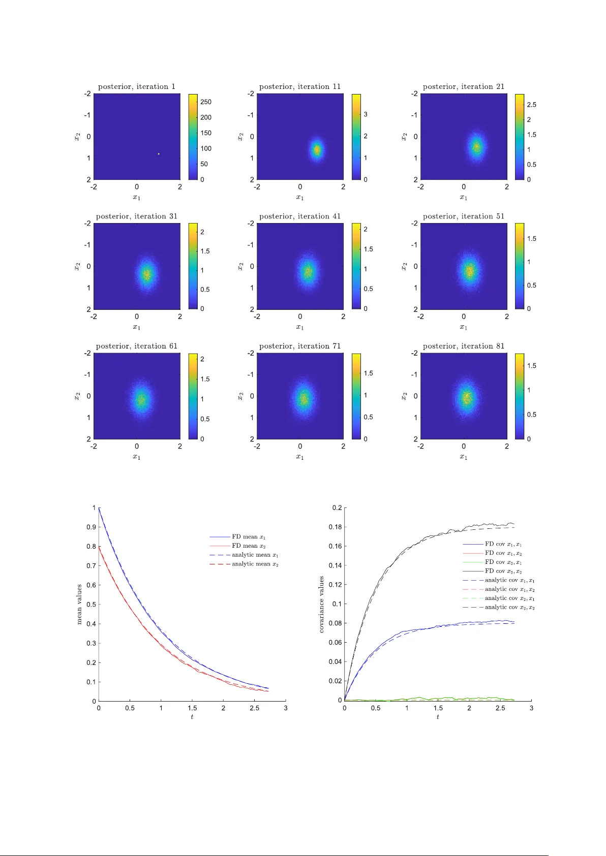
A Full-Density Approach to Simulating Random Iteration Equations with Applications

A F ull-Densit y Approac h to Sim ulating Random Iteration Equations with Applications — Original Researc h Article W olfgang Ho egele 1 1 Munic h Univ ersit y of Applied Sciences HM Departmen t of Computer Science and Mathematics Lothstraße 64, 80335 M ¨ unc hen, German y corresp onding mail: wolfgang.hoegele@hm.edu OR CID: 0000-0002-5303-9334 Marc h 31, 2026 Abstract The goal of this study is to in tro duce a unified computational framework for simulating random iteration equations (RIE), understo o d as iteration equations containing random v ariables. The nov elty of this w ork is that full probability densities of the state vectors are propagated stepwise through the iterations a v oiding the need of repetitive pathwise Mon te Carlo sim ulations of the iteration equation. The pre- sen tation of the metho dology is conceptually efficient based on recent work on static random equations and inten tionally accessible. The technical requirements on the RIE are minimal based on the previous w ork, allowing for potential nonlinearities, discontin uities and sto chasticities in the transfer function, as well as nonstandard densities and diffusion pro cesses. As results, illustrative applications of random and sto chastic differential equation simulations, a no v el full-density gradient descen t metho d (FDGD) for global optimization under uncertain ty and examples of c haotic mappings are presented in order to demonstrate the breadth of the utilit y of this framew ork. In total, the character of the presentation is explorativ e and encourages new applications and theoretical studies. Keyw ords: random iteration equation, density propagation, uncertain t y quantification, sto chastic dy- namics, full-densit y gradien t descen t, sto c hastic differen tial equation, sim ulation Con ten ts 1 In tro duction 3 2 Metho ds 4 2.1 General F ormulation . . . . . . . . . . . . . . . . . . . . . . . . . . . . . . . . . . . . . . . 4 2.2 Numerical Implemen tation . . . . . . . . . . . . . . . . . . . . . . . . . . . . . . . . . . . . 4 2.3 Discretization of Dynamical Systems with Sto c hasticit y as Random Iteration Equation . . 5 2.4 F ull-Density Gradient Descent as Random Iteration Equation . . . . . . . . . . . . . . . . 6 3 Results 7 3.1 Ev olution of Dynamical Systems . . . . . . . . . . . . . . . . . . . . . . . . . . . . . . . . 7 3.2 Optimization with F ull-Density Gradient Descent . . . . . . . . . . . . . . . . . . . . . . . 9 3.3 Chaotic Random Iterations . . . . . . . . . . . . . . . . . . . . . . . . . . . . . . . . . . . 11 4 Discussion 12 5 Conclusion 17 6 App endix 18 6.1 Numerical V erification with the 2D Ornstein-Uhlenbeck SDE . . . . . . . . . . . . . . . . 18 Ab out the Author Dr. H¨ ogele is Professor of Applied Mathematics and Computational Science at the Department of Com- puter Science and Mathematics at the Munic h Univ ersity of Applied Sciences HM, German y . His researc h in terests are mathematical and sto chastic mo deling, sim ulation and analysis of complex systems in applied mathematics with sp ecific applications to radiotherap y , imaging, optical metrology and signal pro cessing. 1 In tro duction In this w ork a no vel computational framew ork is presented to inv e stigate the ev olution of r andom iter ation e quations (RIE). In general, first order iteration equations are transforming a state v ector x ∈ R R starting from an initial state x (1) with a stepwise iteration mapping from the n -th iteration state x ( n ) to the ( n +1)- th iteration state x ( n +1) . This is denoted b y the transfer function T : R R → R R with x ( n +1) = T ( x ( n ) ). RIEs will be defined as iteration equations that contain r andom variables , i.e. T contains sto chasticities summarized by random v ariables in the iteration equation and, in consequence, the resulting next state x ( n +1) m ust also b e interpreted as a random v ariable with a probabilit y density . This means, the RIE gets the density function of a previous state and computes the density function of the next state by incorp orating the random v ariable densities in the transfer function. In total, w e are observing the stepwise evolution of state pr ob ability density functions from iteration to iteration, b eing an example of a density pr op agation algorithm [1, 2]. The prop osed framew ork shows how these density functions can b e computed in practice which is demonstrated by expressiv e examples. RIEs can b e regarded as a key comp onen t for the simulation of many dynamical systems that transform densit y functions, which places this study in the broad field of unc ertainty quantific ation [3]. A minor p oint in this argumentation, but a ma jor difference in the application, is that also the initial state x (1) will b e treated as a random v ariable, i.e. the iteration b egins not with single starting v alues, but with a full distribution of them. In order to understand the broader relev ance of having such a computational framework, this sto chastic extension is presented for three ma jor application areas of iteration equations in applied mathematics: sim ulation of dynamical systems (including r andom and sto chastic differ ential e quations ), optimization (extending gr adient desc ent optimization to a ful l-density gr adient desc ent metho d) and c haotic maps (presen ting the strange attractors of the Ike da map and the L ozi map ). In no wa y this is the full p oten tial of this framew ork, instead it just shows its relev ance for undeniably imp ortan t areas in applied mathematics utilizing expressiv e example sim ulations. Standard approac hes to simulate dynamics depending on uncertainties or diffusion processes are p er- forming statistical pathwise Monte Carlo simulation, i.e. from all probabilit y densities a single sample is dra wn and the corresp onding deterministic iteration is p erformed. This path wise approac h is p erformed in rep etition and all results are collected statistically in a histogram map in order to see the final density of paths [4, 5]. This is not an evolution or propagation of probability densities, but a purely statistical approac h. Based on a recen t publication b y Hoegele [6] whic h focused on a method to compute the proba- bilistic solution space of r andom e quations , the propagation of the probability densities can b e p erformed directly b y computing the full state densit y from iteration to iteration considering the complete sto chastic en vironmen t. Although in the n umerical framew ork w e utilize Mon te Carlo integration techniques, this should not b e misin terpreted with the statistical collection of path wise Mon te Carlo sim ulations. It is clearly stated, that this paper presen ts a simulation framework as men tioned prominen tly in the title with explorative and expressive sim ulation examples in order to present the capabilities of this computational framework. It is not deriving limit theorems, conv ergence rates and theoretical b ounds. Ma jor contributions on this theory is done with the closely related concept of iter ate d r andom functions whic h are studied mainly for the existence of stationary distributions utilizing Lipschitz contraction argumen ts [7, 8], while our approac h is fo cusing on the tr ansient phase and explicit ev olution of the densit y propagation through stepwise nonlinear iterations. Sp ecifically , this study demonstrates that the densit y propagation of sto c hastic and dynamic iteration problems can be sim ulated straightforw ardly , ev en if the theoretical treatment might b e enormously difficult or conv ergence is not guaranteed or (partially) violated. In our p ersp ective, this is more aligned with real world applications in which mostly only a limited num b er of iterations are of computational interest. Moreov er, we typically utilize normal distributions for the parameter random v ariables or diffusion pro cesses, but this is not a limitation of the computational framework and non-standard probability densities (also non-standard diffusion pro cesses) com bined with significant nonlinearities or discontin uities or without Lipsc hitz contraction prop erties of the transfer mapping are as easily handled within this framework as more well-studied situations. F or example, sp ecifically with resp ect to sto chastic differen tial equations this approac h is therefore a computational complement to Perr on-F r ob enius-Op er ator approac hes (which are typically applied to de- terministic, non-random transfer functions and focus on the limiting density) and F okker-Planck-Equation approac hes (which are difficult to apply if contin uous-time Gaussian diffusion pro cesses or smo oth drift or diffusion co efficien ts are not guaran teed). And on the computational side it is also complementary to p athwise Monte Carlo simulations due to the fo cus on ful l-density pr op agation . 3 2 Metho ds 2.1 General F orm ulation W e in tro duce the r andom iter ative e quation (RIE) with a (t ypically at least) piecewise con tin uous transfer function T : R R × R K → R R and a random v ariable parameter vector C ( n ) with K entries and known densities (dep ending on the iteration n um b er n ) by x ( n +1) = T ( x ( n ) , C ( n ) ) , (1) giv en an initial state x (1) ∼ f x (1) . W e wan t to utilize the metho dology recently in tro duced by Hoegele [6] to rewrite this into the standard r andom e quation form M ( x ; A ) = B with indep enden t random v ariable v ectors A and B , and x the corresp onding solution ve ctor . W e transform the iteration equation x ( n +1) − T ( x ( n ) , C ( n ) ) = 0 (2) leading to B a random v ariable v ector cen tered around zero and with small standard deviations compared to other standard deviations and the required solution vector x ( n +1) for each iteration. The rather tec hnical minimal assumptions ab out T are inherited directly from the integrabilit y assumptions ab out M presented in [6] and are typically only violated in constructed limit cases. In total, this leads to M : R R × R R + K → R R (3) M ( x ( n +1) ; x ( n ) , C ( n ) | {z } =: A ) := x ( n +1) − T ( x ( n ) , C ( n ) ) (4) with A := ( x ( n ) 1 , . . . , x ( n ) R , C ( n ) 1 , . . . , C ( n ) K ) T the random v ariable v ector consisting of tw o parts where x ( n ) is a R -dimensional random v ector with densit y f x ( n ) computed in the n -th iteration, and C ( n ) a static K -dimensional random vector with i.i.d. C (1) 1 , . . . , C ( n ) 1 ∼ f C 1 for the first en try , until i.i.d C (1) K , . . . , C ( n ) K ∼ f C K for the last entry . The common densit y function is denoted by f C . F or a well- defined iteration a starting density f x (1) m ust b e defined. The indep endency of the C ( n ) i for different n is directly in the spirit of deterministic iteration equations, where the transfer function itself is indep endent of previous ev aluations of it. Since x ( n ) and C ( n ) are indep enden t, we get a likelihoo d distribution for x ( n +1) based on those densities and the sp ecific transfer function T by L x ( n +1) ( 0 | x ) = Z R K − R Z R R f B ( x − T ( s 1 , s 2 )) · f x ( n ) ( s 1 ) · f C ( s 2 ) d s 1 d s 2 . (5) whic h general form w as presented previously [6]. When fo cusing on probability densities, we reformulate the likelihoo d function with Bay es’ theorem to a p osterior density b y utilizing a non- or w eak-informativ e prior in this study whic h do es not in teract with the lik eliho od intensities by π x ( n +1) ( x ) ∝ L x ( n +1) ( 0 | x ) , (6) essen tially normalizing the lik eliho od function to an integral v alue of 1. In consequence, w e can calculate in each iteration the p osterior density function f x ( n +1) := π x ( n +1) , evolving from a prior starting density f x (1) := π x (1) . Of course, in each iteration there could also b e a density mo difying prior utilized which strongly influences the densit y propagation. This could be imp ortan t, for example, if the state space is restricted b y hard or soft boundaries (utilizing a uniform prior in the region of admissible solutions) and/or is a discrete space with discrete probability densities (utilizing a gridded prior). W e will leav e suc h interesting p ossibilities outside of this study (although it is not outside of the framework) and only refer to the corresp onding Section 2.5 in Ho egele [6]. 2.2 Numerical Implemen tation The main goal of this w ork is to present a computational framew ork for calculating the iterations of the RIE. As presented by Ho egele [6], the in tegral in Equation 5, can b e approximated by Mon te Carlo 4 in tegration, utilizing P samples with the formula π x ( n +1) ( x ) ∝ 1 P P X p =1 R Y r =1 f B r ( x r − T r ( s 1 ,p , s 2 ,p )) ! , (7) where the samples s 1 ,p are drawn form the density π x ( n ) and s 2 ,p are drawn from f C ( n ) . The sampling for the latter is straigh tforward, since these are giv en b y the RIE definition and one can for example utilize latin hyp er cub e sampling (even the same representativ e samples for all iterations once calculated b efore iterations start). The sampling of the first density π x ( n ) m ust b e done in each iteration and these densities are non-trivial. There are standard Monte Carlo Markov Chain (MCMC) metho ds in order to draw from such p osteriors, but in this work we prefer due to simplicity an ac c eptanc e r eje ction approac h [4]. Essen tially , drawing in a R -dimensional rectangular b ox around the density region of π x ( n ) ( x ) uniformly distributed samples x p with one additional uniform sample y p in the range of 0 and the maximum ov erall v alue of π x ( n ) . If y p is larger than π x ( n ) ( x p ) it is rejected, else it is k ept. This is done in parallelization for sp eed-up and exactly P samples are computed in eac h iteration. A p ossible schematic algorithm (whic h is also the basis of the presen ted results) lo oks lik e 1. Define the RIE, esp ecially the transfer function T : R R × R K → R R , the i.i.d. random v ariable densities f C and the initial prior densit y π x (1) . Set n = 1. 2. T ake P draws s 2 ,p ( p = 1 , . . . , P ) from f C b y standard sampling metho ds (e.g. by latin hyp er cub e sampling). 3. T ake P draws s 1 ,p ( p = 1 , . . . , P ) from π x ( n ) (e.g. by ac c eptanc e r eje ction ). 4. Ev aluate Equation 7 n umerically in order to calculate π x ( n +1) (including the normalization step of the appro ximated densit y) on the same grid as π x ( n ) w as pro vided. 5. Set n → n + 1 and rep eat steps 3–5 un til a certain limit has b een reached, suc h as a given iteration n um b er or the c hanges b et ween π x ( n ) and π x ( n +1) are b elo w a certain tolerance measure. This algorithm for simulating full densities of the RIEs can be applied directly for the stochastic extension of a giv en iteration equation, such as the c haotic mappings presented in the results Section 3.3. More imp ortan t in applied mathematics are situations where the iteration equation itself (and its sto chastic extension to RIE) is a to ol to solve challenging (mostly nonlinear) problems. W e will present t w o of the most prominen t use cases in the next subsections. 2.3 Discretization of Dynamical Systems with Sto c hasticit y as Random It- eration Equation W e will see, that being able to simu late RIEs are a k ey step to sim ulate appro ximately r andom differ ential e quation (RDE) and sto chastic differ ential e quation (SDE) dynamical systems in order to observe their ev olution of the full densities ov er time [9, 5]. W e are starting applications with a general ODE system with random v ariable parameters C , representing a RDE, ˙ x = F ( t, x , C ) , (8) with a well-defined right hand side F . By applying the discretization ˙ x ≈ x ( n +1) − x ( n ) ∆ t , this leads to the iteration equation x ( n +1) = x ( n ) + ∆ t · F ( t n , x ( n ) , C ( n ) ) , (9) essen tially representing a random Euler iter ation equation. When using the nomenclature of Section 2.1, this leads to the general transfer function T ( x ( n ) , C ( n ) ) := x ( n ) + ∆ t · F ( t n , x ( n ) , C ( n ) ) , (10) for an arbitrary dynamical system. Of course, more adv anced discretization schemes can b e utilized, but for simplicit y w e lea v e this demonstration applying the Euler algorithm. 5 A ma jor observ ation is that when utilizing this discretization scheme, w e can also sim ulate the evolution of probabilit y densit y functions of SDEs with random coefficients utilizing the Euler-Maruyama algorithm [4, 5, 10] b y in tro ducing new terms x ( n +1) = x ( n ) + F ( t n , x ( n ) , C ( n ) ) ∆ t + B ( t n , x ( n ) , D ( n ) ) ∆ W ( n ) , (11) with the diffusion co efficien t function B ( t n , x ( n ) , D ( n ) ), which may dep end on a random v ariable vector D ( n ) , and a Wiener pro cess W t with a discrete increment ∆ W ( n ) = W t n +1 − W t n as normally distributed random v ariables with zero mean and v ariances ∆ t . This leads to the general transfer function for SDEs T ( x ( n ) , C ( n ) ) := x ( n ) + F ( t n , x ( n ) , C ( n ) 1 ..K 1 ) ∆ t + B ( t n , x ( n ) , C ( n ) K 1 +1 ..K 1 + K 2 ) C ( n ) K 1 + K 2 +1 ..K 1 + K 2 + R , (12) with three parts of C , i.e. the K 1 random v ariables of the drift co efficient C 1 ..K 1 , the K 2 random v ariables of the diffusion coefficient C K 1 +1 ..K 1 + K 2 and the R random v ariables of the discrete increment in the Wiener pro cess C K 1 + K 2 +1 ..K 1 + K 2 + R . Please note, that Equation 12 is a general model including parameter uncertain ties (the RDE part) as w ell as a diffusion pro cess (the SDE part) in one single computational framew ork. This shows already from the metho dological side the p ow er of the RIE approac h for appro ximating those in general challenging pro cesses combined. Additionally , it can b e observed that if C ( n ) (and resp ectively D ( n ) ) of Equation 11 are indep enden t (but not necessarily iden tically distributed) for different n then also more complicated co efficien t pro cesses can be sim ulated just b y reinterpretation of the terms (not lea ving the computational framew ork). This exemplifies the conceptual similarities b et w een RDEs and SDEs, esp ecially from a sim ulation p ersp ective. F urther, the SDEs are not limited to Wiener pro cesses, but can in the simulation tak e an y other sto chastic process that increment can be calculated for eac h iteration (which is deliberately general and leav es a lot of p ossibilities). Finally , also more sophisticated approaches than the simplistic Euler-Maruyama algorithm can b e utilized for SDE sim ulation, without lea ving the presented general framew ork as long as they lead to iteration equations. F or the conv ergence rates of standard SDE t yp es for the Euler-Maruyama algorithm see e.g. Higham[10]. Ob viously , this strict fo cus on the discretized iteration equation as the k ey quantit y op ens up many p ossibilities for simulating challenging RDEs and SDEs b esides the standard theory and curren t research in their fields. In this study , this is only regarded as one example application of RIE simulations. 2.4 F ull-Densit y Gradient Descen t as Random Iteration Equation The idea of gradien t descent is to update a current position x ( n ) in a minimization process of an ob jective function F ( x ) with F : R R → R step wise in the direction of the steep est do wnw ard direction which is represen ted b y the negativ e direction of the lo cal gradien t, i.e. leading to the gradien t descen t (GD) algorithm x ( n +1) = x ( n ) − η · ∇ F ( x ( n ) ) , (13) with a le arning r ate η . W e present sev eral sto chastic extensions to this classical optimization routine, whic h family will b e denoted with ful l-density gr adient desc ent (FDGD): 1. FDGD-I: Minimization of a sto c hastic ob jective function containing K random v ariables for pa- rameters of the ob jective function x ( n +1) = x ( n ) − η · ∇ F ( x ( n ) , C ( n ) ) (14) In this v ersion sto chastic optimization is p erformed, i.e. we hav e an ob jective function containing random v ariable parameters. W e just w ant to present this approach here since it is an obvious v ersion, but are not studying it in detail further on. 2. FDGD-I I: Minimization of a deterministic ob jectiv e function up dating the deterministic direction sim ultaneously for a full densit y of directions, leading to R random v ariables x ( n +1) = x ( n ) − η · ∇ F ( x ( n ) ) + C ( n ) (15) This approach introduces a diffusion process in to the iteration whic h helps exploring the ob jective function. 6 3. FDGD-I I I: Additionally to FDGD-I I the update utilizes a full density of learning rates, leading to R + 1 random v ariables x ( n +1) = x ( n ) − C ( n ) R +1 · ∇ F ( x ( n ) ) + C ( n ) , (16) leading to an up date with differen t optimization sc hemes sim ultaneously . FDGD-I I and FDGD-I I I contain a diffusion comp onent due to the added random v ariables in each itera- tion with a simultaneous con vergence to local minima, pro ducing complex dynamics during optimization. This leads, for example, to the transfer function for FDGD-I I I T ( x ( n ) , C ( n ) ) := x ( n ) − C ( n ) R +1 · ∇ F ( x ( n ) ) + C ( n ) , (17) and for the other FDGD schemes analog. Again, this formulation is very general for any differen tiable ob jective function F . In addition, combining FDGD-I and FDGD-II I addresses an extremely broad set of sto c hastic optimization problems, transforming the lo cal gradient descen t algorithm to a glob al sto chastic optimization tec hnique. The difference to sto chastic gr adient desc ent (SGD) in the literature is that we do not use a single realization of the stochastic path in each iteration (whic h in SGD is produced b y subsets of data for calculating the gradient in mac hine learning) but the whole densit y functions are transformed which allows a muc h broader search [11]. Related ideas of density propagation b y sto c hastic gradien t descen t [12] and for the connection of SDEs and gradient descen t [13] are part of recent researc h. W e further wan t to draw the attention to the strong similarities of SDEs and the FDGD approach within the RIE framew ork whic h ma y lead to further insights. 3 Results 3.1 Ev olution of Dynamical Systems W e present tw o versions of one dynamical system example. First, the normalized R osenzweig McA rthur as a RDE mo del [14, 15, 16] for predator prey sim ulations is giv en b y ˙ x 1 = x 1  1 − x 1 C 1  − C 2 x 1 x 2 1 + x 1 (18) ˙ x 2 = − C 3 x 2 + C 2 x 1 x 2 1 + x 1 , (19) with the random v a riables representing uncertainties ab out the parameters of the mo del. The straigh t- forw ard discretization ˙ x ≈ x ( n +1) − x ( n ) ∆ t leads to the transfer function T ( x ( n ) , C ( n ) ) :=     x ( n ) 1 + ∆ t ·  x ( n ) 1  1 − x ( n ) 1 C ( n ) 1  − C ( n ) 2 x ( n ) 1 x ( n ) 2 1+ x ( n ) 1  x ( n ) 2 + ∆ t ·  − C ( n ) 3 x ( n ) 2 + C ( n ) 2 x ( n ) 1 x ( n ) 2 1+ x ( n ) 1      (20) In the simulation, w e utilize indep endent Gaussian densities f C 1 := N (1 , 0 . 01 2 ), f C 2 := N (1 , 0 . 01 2 ) and f C 3 := N (0 . 25 , 0 . 01 2 ) as well as f B 1 , f B 2 := N (0 , 0 . 005 2 ). The differential equation mo del is known to lead to a steady state density [16] and we w an t to observe the evolution of the starting distribution to this steady state distribution based on the discretized iteration equation. W e utilize P = 192000 samples and ∆ t = 0 . 2 (observing acceptable conv ergence results with minor numerical artifacts, see Figure 3 (left) for an impression). In Figure 1, we are utilizing starting density f x (1) as a uniform densit y on [0 . 1 , 0 . 5] × [0 . 1 , 0 . 5] and observ e its evolution into the steady state distribution. The deterministic steady state (when taking the modes of eac h densit y function as parameter v alues) is at ( 1 3 , 8 9 ) and coincides w ell with the sim ulation result. In the second example, we present a SDE version of the normalized R osenzweig McArthur mo del [19], i.e. d x 1 =  x 1  1 − x 1 k  − m x 1 x 2 1 + x 1  d t + σ 1 x 1 d W 1 (21) d x 2 =  − c x 2 + m x 1 x 2 1 + x 1  d t + σ 2 x 2 d W 2 , (22) 7 Figure 1: Illustration of the p osterior densities for different iteration n umbers of the Rosenzweig McArthur RDE mo del. One can see the evolution of the square uniform initial density and how it evolv es due to the dynamics of the Rosenberg McArth ur mo del with random v ariable parameters to the steady state densit y . 8 with the real parameters k , m, c and a Wiener pro cess W t , leading to the transfer function T ( x ( n ) , C ( n ) ) :=     x ( n ) 1 +  x ( n ) 1  1 − x ( n ) 1 k  − m x ( n ) 1 x ( n ) 2 1+ x ( n ) 1  ∆ t + σ 1 x ( n ) 1 C ( n ) 1 x ( n ) 2 +  − c x ( n ) 2 + m x ( n ) 1 x ( n ) 2 1+ x ( n ) 1  ∆ t + σ 2 x ( n ) 2 C ( n ) 2     . (23) In this simulation w e utilize a parameter set which leads to perio dical orbits in the x 1 - x 2 -space in the deterministic case with k = 1 . 9 , m = 1 . 1 , c = 0 . 31, but add the sto c hastic noise densities f C 1 , f C 2 := N (0 , ∆ t ) of the discritized SDE and use scaling co efficients σ 1 = σ 2 = 0 . 04. In Figure 2 w e utilize P = 384000 samples and ∆ t = 0 . 05 (leading to the observ ation of a clear orbital structure with minor n umerical artifacts, see Figure 3 (right) for an impression) and present in the plot representativ e density functions (iteration 476 to 780) roughly ov er one p erio d of the orbit. The p eriodicity is not p erfect since the parameter v alues are a compromise for the p erio dicity of the full starting v alue range (which lead also to sligh tly differen t perio dicities, see Figure 3 (right)) and the SDE diffusion leads to broad distributions of the orbital state densit y . Still, a clear orbit is observ able also in this SDE v ersion and it is demonstrated that suc h challenging simulations can b e p erformed based purely on the computational framew ork of iterativ e densit y transformations. An additional v erification of the full-density sim ulation is provided in App endix Section 6.1 where the sim ulation results are compared to the evolution of the analytically known mean and cov ariances of a 2D Ornstein-Uhlen b ec k type SDE. 3.2 Optimization with F ull-Densit y Gradien t Descen t W e present t w o expressive ob jective functions in order to demonstrate the use of this metho dology for gradien t descent. First, we present an ob jective function with t w o lo cal minima and one saddle p oint in b et ween F ( x ) = x 4 1 − 3 x 2 1 + x 1 + 5 + 2 x 2 2 , (24) presen ted in Figure 4 on the left side with ∇ F ( x ) =  4 x 3 1 − 6 x 1 + 1 4 x 2  , (25) and apply the FDGD-I I algorithm, leading to the transfer function T ( x ( n ) , C ( n ) ) :=    x ( n ) 1 − η ·  4  x ( n ) 1  3 − 6 x ( n ) 1 + 1  + C ( n ) 1 x ( n ) 1 − η ·  4 x ( n ) 2  + C ( n ) 2    . (26) Second, we presen t the famously challenging Himmelblau’s ob jectiv e function [18, 13] with four minima whic h are difficult to lo calize F ( x ) = ( x 2 1 + x 2 − 11) 2 + ( x 1 + x 2 2 − 7) 2 , (27) presen ted in Figure 4 on the righ t side with ∇ F ( x ) =  4 x 1 ( x 2 1 + x 2 − 11) + 2 ( x 1 + x 2 2 − 7) 2 ( x 2 1 + x 2 − 11) + 4 x 2 ( x 1 + x 2 2 − 7)  , (28) and apply the FDGD-I II algorithm, leading to the transfer function T ( x ( n ) , C ( n ) ) :=     x ( n ) 1 − C ( n ) 3 ·  4 x ( n ) 1   x ( n ) 1  2 + x ( n ) 2 − 11  + 2  x ( n ) 1 +  x ( n ) 2  2 − 7  + C ( n ) 1 x ( n ) 1 − C ( n ) 3 ·  2   x ( n ) 1  2 + x ( n ) 2 − 11  + 4 x ( n ) 2  x ( n ) 1 +  x ( n ) 2  2 − 7  + C ( n ) 2     . (29) 9 Figure 2: Illustration of the p osterior densities for different iteration n umbers of the Rosenzweig McArthur SDE mo del. The evolution of the densities is presen ted roughly ov er one p erio d of the orbit in the x 1 - x 2 -space starting at iteration 476 ( t = 23 . 8), with dominant sto chastic effects due to the SDE diffusion and initial state densit y . 10 Figure 3: Numerical impression of step sizes for the discretization of the dynamic systems by deterministic sim ulations in the relev ant time and initial v alue range (t w o starting v alue examples, whic h are vertices of eac h initial densit y box) with o de45 ( Runge-Kutta-(4,5) algorithm) as ground truth and the Euler algorithm which is basis of the simulaion strategy . Left: for system 1 utilized in the simulation in Figure 1 with starting v alues (0 . 1 , 0 . 1) and (0 . 5 , 0 . 5), right: for system 2 utilized in the simulation in Figure 2 with starting v alues (0 . 4 , 0 . 4) and (0 . 6 , 0 . 6). Sufficient numerical approximation accuracy in the con text of this study can b e observ ed considering the sim ulated sto c hasticities. In Figure 5, for the first ob jective function (Figure 4, left) w e utilize independent Gaussian densities f C 1 := N (0 , 0 . 04 2 ) and f C 2 := N (0 , 0 . 04 2 ) as well as f B 1 , f B 2 := N (0 , 0 . 02 2 ) and P = 48000 samples. This FDGD-I I example with learning rate η = 0 . 075 with a small starting densit y shows ho w the gradient descen t is attracted b y the saddle p oin t first and afterw ards conv erges simultaneously to the tw o minima. In Figure 6, for a FDGD-I I I example with the second ob jective function (Figure 4, right) w e utilize f C 1 := N (0 , 0 . 2 2 ), f C 2 := N (0 , 0 . 2 2 ) as w ell as f B 1 , f B 2 := N (0 , 0 . 02 2 ) and the learning rate density f C 3 := N (0 . 01 , 0 . 003 2 ) (using P = 384000 samples). Starting with a broad density , we see the fast attraction by a broad searc h for the p osterior to the four minima. This shows, that in this stochastic regime an unsp ecific search strategy can b e b eneficial finding challenging extrema in a simultaneous fashion. 3.3 Chaotic Random Iterations W e again present tw o n umerical examples for this class of applications. Since chaotic random iterations are already applicable in the standard form ulation of Section 2.1, w e use the presen ted framew ork directly . First, the classical Ike da map [19] in real space is presented by x ( n +1) 1 = 1 + u · ( x ( n ) 1 · cos( t ( n ) ) − x ( n ) 2 · sin( t ( n ) )) (30) x ( n +1) 2 = u · ( x ( n ) 1 · sin( t ( n ) ) + x ( n ) 2 · cos( t ( n ) )) , (31) with t ( n ) = 0 . 4 − 6 1 +  x ( n ) 1  2 +  x ( n ) 2  2 . (32) 11 Figure 4: Illustration of the ob jectiv e function. Left: With tw o local minima on the x 1 -axis. Right: Himmelblau’s function of optimization for four lo cal minima. Dep ending on the parameter u different strange attractors app ears. W e are exploring the RIE for a small range of the v ariable C ( n ) 1 = u represen ted b y a random v ariable leading to the transfer function T ( x ( n ) , C ( n ) 1 ) := 1 + C ( n ) 1 · ( x ( n ) 1 · cos( t ( n ) ) − x ( n ) 2 · sin( t ( n ) )) C ( n ) 1 · ( x ( n ) 1 · sin( t ( n ) ) + x ( n ) 2 · cos( t ( n ) )) ! . (33) In Figure 7 w e explore the progress of iterations for f C 1 := N (0 . 7 , 0 . 02 2 ) with P = 384000. It can b e observ ed that the strange attractor arises during iterations, but also how the Ikeda mapping b ehav es in its first iterations acting on a full starting densit y distribution. This is an a verage of the strange attractor according to the ensem ble distribution of the u -parameter (= C ( n ) 1 ). Second, the classical L ozi map [20] is presented, which is given by x ( n +1) 1 = 1 − a · | x ( n ) 1 | + x ( n ) 2 (34) x ( n +1) 2 = b · x ( n ) 1 , (35) with t ypically a fixed standard parameter b = 0 . 3 and a range for a ∈ [1 . 4 , 1 . 7] for which strange attractors app ear. This can b e transferred to the transfer function T ( x ( n ) , C ( n ) 1 ) := 1 − C ( n ) 1 · | x ( n ) 1 | + x ( n ) 2 b · x ( n ) 1 ! , (36) b eing an example for a non-differentiable transfer function. In Figure 8 we explore the progress of iterations for f C 1 := N (1 . 55 , 0 . 1 2 ) with P = 3840 00. Also in this case the characteristic strange attractor with its sharp edges can b e observ ed, ev en if w e utilize a full ensem ble of a parameters. 4 Discussion In this explorative study we inv estigated a nov el computational framew ork for RIE. This work is mainly based on the pap er by Ho egele [6], which demonstrated ho w to calculate the probability density of the solutions space of (static and nonlinear) random equation systems. The main idea in this pap er is now to utilize this metho dology in an iterative fashion, leading to dynamics of probability density propagations. Essen tially , the iteration transforms in each step the starting density function com bined with the random v ariables contained in the iteration function itself in order to compute the next iteration state density . This can b e regarded as computing ensemble solutions for dynamical systems, e.g. [21]. 12 Figure 5: Illustration of the p osterior densities for different iteration num b ers for FDGD-I I for the ob jective function with t wo lo cal minima. One can see the evolution of the square initial density b eing first attracted to the saddle p oin t and second the con v ergence to the t w o lo cal minima. 13 Figure 6: Illustration of the p osterior densities for different iteration num b ers for FDGD-I I I using Him- melblau’s test ob jectiv e function. One can see the ev olution of the broad circular initial density with a v ariation of the up date rate and its fast con v ergence to the four lo cal minima. 14 Figure 7: Illustration of the p osterior densities of the Ike da mapping . One can see the ev olution of the broad square initial density into the characteristic strange attractor of the Ik eda mapping av eraged ov er a densit y of the u -parameter. 15 Figure 8: Illustration of the p osterior densities of the L ozi mapping . One can see the evolution of the broad square initial density into the strange attractor of the Lozi mapping with sharps edges a v eraged o v er a densit y of the a -parameter. 16 A ma jor difference compared to path wise Monte Carlo simulations is that the full density of the state space is calculated in eac h iteration step instead of several deterministic paths whic h are av eraged after- w ards. An adv antage could b e the adaptive and more efficient sampling of the o ccurring densities during sim ulation, since in the path wise approac h only after the full simulations the densities appear statistically . As all iterativ e schemes, RIEs show interesting prop erties. This is demonstrated by the application to sto c hastic dynamical systems, such as RDEs and SDEs, whic h sho w non trivial evolutions of the state densities. W e also show how this framework can b e used for an explorative gradient descent, whic h w e denote by FDGD ( ful l-density gr adient desc ent ) as a p ow erful extension of classical gradient descen t to glob al optimization . Essen tially , this leads to a meaningful search strategy for many local minima simultaneously with decisions taken not by single random paths but for a whole density of searc h directions. In this con text, sto chastic gr adient desc ent [11] could be associated with single random path of optimization and ensemble optimization with the tracking of a num b er of sample paths in parallel during iterations, but not the full density . W e wan t to emphasize that the presen ted simulation of dynamical systems and optimization are t w o main applications of applied mathematics, and utilizing RIEs allows a straigh tforw ard extension to stochastic regimes. Finally , we provide an impression ho w strange attractors in c haotic mappings are computed with this framework for full densities of starting v alues and parameters. This is the most direct application of the framework. Another imp ortan t task in applied mathematics is solving nonlinear equation systems, e.g. by Newton’s metho d or similar approaches, which typically lead in the deterministic case also to iteration equations. Since solving static equations (without a dynamic comp onent) was already completely addressed in Ho egele [6] b y the general nonlinear form M ( x ; A ) = B without the need of iteration equations, the extension to this computational framew ork is not necessary and it is referred to the pap er. The most imp ortant p oint of the presentation of this framework is that it is simple (if there is a metho d to solve static random equations) and very general, and it should b e applicable to many dynamics whic h are based on iterations (explicitly focusing on discretized con tinuous phenomena). As a side note, in dynamical systems the time step ∆ t could also b e tak en as random v ariable (similar to the learning rate in FDGD-II I), represen ting differen t discretization sc hemes of the dynamical system sim ultaneously . This leads to a new understanding of the simulation of dynamical systems, allowing to sto chastically explore the discretization metho d itself. In general, com bining the tw o areas, discretized dynamical systems and gradien t optimization within the RIE framew ork ma y lead to new insights in b oth areas. This study is explorative and not a deriv ation of theoretical b ounds or conv ergence rates of numerical sc hemes, which are imp ortant on their own and complementary to this presentation. Instead this study explores the p ossibilit y to approximately compute and visualize the evolution of a finite num b er of iterations. W e regard this fo cus as underrepresented in the study of sto c hastic dynamical systems which is a ma jor part of the motiv ation of this work. Due to this sp ecific fo cus, this approac h should be regarded in the mindset of unc ertainty quantific ation in the broad field of scientific c omputing , where uncertainties are propagated through dynamical systems b y sim ulation and their impact is quantified in the results. There are several dimensions to further develop the application of the framework: a) more efficient n umerical sc hemes for sampling the densit y functions in the Monte Carlo in tegration than, e.g. ac c eptanc e r eje ction sampling, b) more efficient use of the definition of the state space grid in the sim ulation, including p ossibly adaptive grids, c) b etter discretization approaches in the deriv ation of the random iteration equations (e.g. for contin uous dynamical systems from Euler algorithm to R unge Kutta algorithms, e.g. [22]) and a detailed inv estigation of their conv ergence rates, d) extension of the optimization approaches, e.g. higher order iterative schemes such as full-densit y Newton optimization, etc., e) more c hallenging parameter density functions apart from normal distributions and a broader (also discontin uous) selection of the transfer functions, f ) going from R = 2 to higher dimensional state spaces and/or random v ariable v ectors, e.g. inv estigating the curse of dimensionality for this approach, and finally , g) extension to other interesting application areas where iteration equations can play a pro ductive role in understanding dynamical phenomena and con tain random v ariable densities as a new degree of freedom in the mo deling pro cess. 5 Conclusion In this paper, a unified framework for the sim ulation of random iteration equations (RIE) via direct prob- abilit y densit y propagation has b een dev elop ed. This is based on recen t work on static random equations, whic h is iteratively applied in this study . In consequence, the algorithmic approach is conceptually ef- 17 ficien t and straightforw ard. Expressive applications, such as the sim ulation of random and sto c hastic differen tial equations, the extension of gradient descen t to the nov el full-density gradien t descent ap- proac h as well as the sim ulation of chaotic maps with strange attractors show case its wide applicabilit y . These demonstrations visualize complex sto chastic evolutions of the simulation results and highlight the framew ork’s p oten tial as a p ow erful to ol for understanding the in terpla y b et w een nonlinear dynamics and sto c hasticities in the field of uncertain ty quan tification. Several future directions of this approac h are discussed. 6 App endix 6.1 Numerical V erification with the 2D Ornstein-Uhlen b ec k SDE F or an indep enden t verification of the SDE calculation, we present a simple 2D Ornstein-Uhlen b ec k SDE d x 1 = − x 1 d t + σ 1 d W 1 (37) d x 2 = − x 2 d t + σ 2 d W 2 , (38) with the real diffusion parameters σ 1 , σ 2 and a Wiener pro cess W t , leading to the transfer function T ( x ( n ) , C ( n ) ) := x ( n ) 1 − x ( n ) 1 ∆ t + σ 1 C ( n ) 1 x ( n ) 2 − x ( n ) 2 ∆ t + σ 2 C ( n ) 2 ! . (39) The sto c hastic noise densities are f C 1 , f C 2 := N (0 , ∆ t ) of the discritized SDE and the diffusion coefficients are σ 1 = 0 . 4 , σ 2 = 0 . 6. In Figure 9 w e utilize P = 384000 samples, f B 1 , f B 2 := N (0 , 0 . 0025 2 ) and ∆ t = 0 . 025 and show the ev olution of the density function. As starting distribution an (almost) p oint distribution at x 0 = (1 , 0 . 8) T is c hosen (please note, we utilized a slightly extended square with size 0 . 045 in order to utilize exactly the same algorithm as in Section 3.1). During this transient phase, the exp ected drift to the zero mean p osition is observ able as well as the anisotropic increase in the diffusion. The analytic solution for the mean M ( t ) and the cov ariance matrix Σ ( t ) for this pro cess is kno wn and giv en b y M ( t ) = x 0 e − t (40) Σ ( t ) = 1 2 (1 − e − 2 t )  σ 2 1 0 0 σ 2 2  . (41) In Figure 10 the n umerical ev aluation of the mean and the cov ariance v alues utilizing the full-density approac h o ver 109 iterations in the transien t phase are compared to the time-dependent analytic solution. The comparison demonstrates an agreemen t with minor differences verifying the calculation. Possible sources for remaining errors are the discretization errors (spatial as well as temp oral utilizing the Euler- Maruy ama approach), the finite num b er of Mon te Carlo samples for in tegration, an extended starting distribution in the simulation instead of a p oin t distribution as for the analytic solution and the slightly diffusing c haracter of the standard deviation of B when solving the random iteration equations. References [1] Li, J., Chen, J. The principle of pr eservation of pr ob ability and the gener alize d density evolution e quation , Structural Safety 30 (2008) 65–77, https://doi.org/10.1016/j.strusafe.2006.08.001. [2] Caluya, K. F., Halder, A. Gr adient Flow Algorithms for Density Pr op agation in Sto chas- tic Systems , IEEE T ransactions on Automatic Control, V olume 65, Issue: 10, 2020. h ttps://doi.org/10.1109/T AC.2019.2951348 [3] Sulliv an, T.J., In tro duction to Uncertain ty Quantification, Springer International Publishing, 2015. DOI: 10.1007/978-3-319-23395-6 [4] Rubinstein R. Y., Kro ese D. P ., Simulation and the Monte Carlo Metho d , 3. Auflage, John Wiley & Sons, 2017 18 Figure 9: Illustration of the p osterior densities for different iteration num b ers of the 2D Ornstein- Uhlen b ec k SDE mo del utilizing the full-density approach. Figure 10: Illustration of the mean and co v ariance v alues empirically ev aluated for the full-density algo- rithm (FD, solid lines) and the analytic solution (dashed lines). The strong similarity b etw een FD and the analytic solution is demonstrated. 19 [5] Klo eden, P . E., Platen, E., Numeric al Solution of Sto chastic Differ ential Equations , Springer Berlin, Heidelb erg, 1992 [6] Ho egele, W. Combinatorial p otential of r andom e quations with mixtur e mo dels: Mo del- ing and simulation , Mathematics and Computers in Sim ulation 239, pp. 696-715, 2026, h ttps://doi.org/10.1016/j.matcom.2025.07.033. [7] Sandri´ c, N. R ademacher le arning r ates for iter ate d r andom functions , Journal of Complexity , V olume 91, h ttps://doi.org/10.1016/j.jco.2025.101971 [8] Diaconis, P ., F reedman D. Iter ate d R andom F unctions . SIAM Review, V ol. 41, Iss. 1, 1999 h ttps://doi.org/10.1137/S0036144598338446 [9] Jornet, M. The ory and metho ds for r andom differ ential e quations: a survey. SeMA 80, 549–579, 2023. h ttps://doi.org/10.1007/s40324-022-00314-0 [10] Higham D. J., An Algorithmic Intr o duction to Numeric al Simulation of Sto chastic Differ ential Equa- tions , SIAM Review, V ol. 43,No. 3,pp. 525–546, Society for Industrial and Applied Mathematics, 2001 [11] Go o dfello w, J., Bengio, Y., Courville, A. De ep L e arning , MIT Press, 2016 [12] Mandt, S., Hoffmann, M. D., Blei, D. M., Sto chastic Gr adient Desc ent as Appr oximate Bayesian Infer enc e , Journal of Machine Learning Research, 18 1-35, 2017 [13] Przyby lo wicz, P ., Sobiera j, M. On the r andomize d Euler scheme for sto chastic differ ential e qua- tions with inte gr al-form drift , Journal of Computational and Applied Mathematics 483, 2026, h ttps://doi.org/10.1016/j.cam.2026.117367 [14] N. Stollen werk, M. Aguiar, B.W. Ko oi, Mo del ling Hol ling typ e II functional r esp onse in deterministic and sto chastic fo o d chain mo dels with mass c onservation , Ecological Complexit y 49, 100982, 2022, h ttps://doi.org/10.1016/j.eco com.2022.100982. [15] Sarah K. Wyse, Maria M. Martignoni, May Anne Mata, Eric F o xall, Reb ecca C . Tyson, Structur al sensitivity in the functional r esp onses of pr e dator–pr ey mo dels , Ecological Complexit y 51, 101014, 2022, h ttps://doi.org/10.1016/j.eco com.2022.101014. [16] Ho egele, W. Ste ady State Distribution and Stability Analysis of R andom Differ ential Equations with Unc ertainties and Sup erp ositions: Applic ation to a Pr e dator Pr ey Mo del , 2026, [math.DS], h ttps://doi.org/10.48550/arXiv.2603.03845 [17] Louis Shuo W ang, Jiguang Y u, Wel l-Pose dness for the R osenzweig-MacArthur Mo del with Internal Sto chasticity , arXiv:2505.16904 [math.PR], 2025, https://doi.org/10.48550/arXiv.2505.16904 [18] Himmelblau, D. Applie d Nonline ar Pr o gr amming . McGraw-Hill, 1972 [19] W ang,M., Yi, Z., Li, Z. A memristive Ike da map and its applic ation in image encryption , Chaos, Solitons & F ractals, V olume 190, 2025, https://doi.org/10.1016/j.c haos.2024.115740 [20] Lozi R. Survey of R e c ent Applic ations of the Chaotic L ozi Map. Algorithms . 2023; 16(10):491. h ttps://doi.org/10.3390/a16100491 [21] Penenk o, A.V., Kazak ov, G.I., Iv anov, K.O. A lgorithms for Appr oximate Solution of ODE En- sembles Using Clustering and Sensitivity Matric es. Numer. Analys. Appl. 18, 157–172 (2025). h ttps://doi.org/10.1134/S1995423925020053 [22] Sadegh Amiri, S. Mohammad Hosseini A class of we ak se c ond or der split-drift sto chastic Runge–Kutta schemes for stiff SDE systems. Journal of Computational and Applied Mathematics 275, 27-43 (2015). h ttps://doi.org/10.1016/j.cam.2014.07.023 20