The Full Set of KMS-States for Abelian Kitaev Models

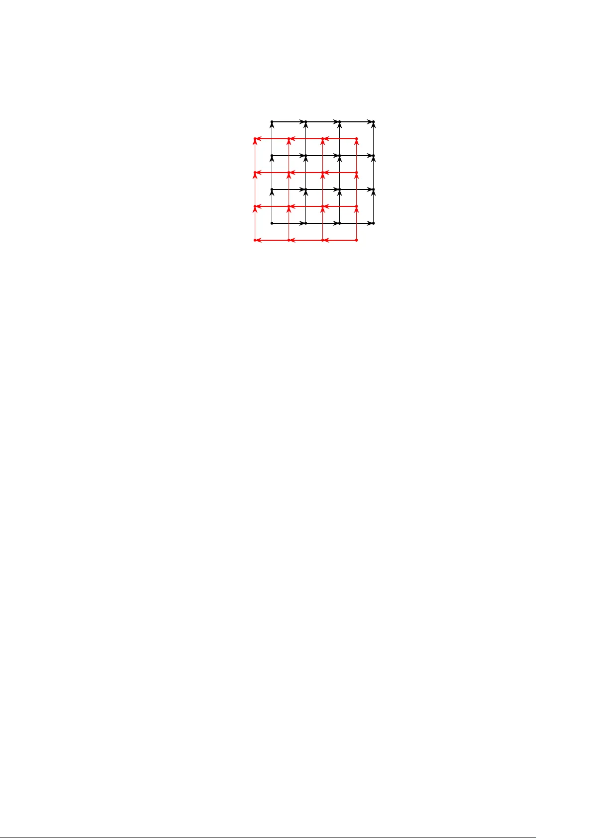
THE FULL SET OF KMS-ST A TES FOR ABELIAN KIT AEV MODELS D ANILO POLO OJITO AND EMIL PR OD AN A B S T R AC T . W e first prov e that the subalgebra C generated by the v ertex and face opera- tors of an abelian Kitaev model is a C ∗ -diagonal of the UHF algebra A of quasilocal ob- servables. This gi ves us access to the W eyl groupoid G C associated with the C ∗ -inclusion C , → A , which supplies a valuable presentation of A as a groupoid C ∗ -algebra where the dynamics of the model are generated by a groupoid 1-cocycle c H . Making appeal to the notion of ( c H , β ) -KMS measures for this groupoid, we identify the full set of KMS states of the model and prove its uniqueness for β ∈ [ 0, ∞ ) . Furthermore, we show that its limit at β → ∞ exists and coincides with the unique frustration-free ground state of the model. MSC 2020 : Primary: 46L55, 82B10; Secondary: 37A55, 22A22, 46L05. Keyw ords : Quantum double models, W eyl gr oupoid, KMS states, C ∗ -diagonals C O N T E N T S 1. Introduction 1 2. C ∗ -Diagonals Generated by Abelian Kitae v Models 3 2.1. Abelian Kitae v models 3 2.2. The commutati ve algebra of local interactions 5 2.3. The C ∗ -diagonal of an Abelian Kitae v model 10 3. The W eyl Groupoids of Abelian Kitae v Models 11 4. The complete set of KMS states 13 4.1. KMS states 13 4.2. KMS measures 14 4.3. The set of KMS states 15 Declarations 21 References 21 1. I N T RO D U C T I O N In his influential paper , A. Kitae v introduced the quantum double models , a class of topologically ordered quantum spin systems defined on triangulations of two-dimensional surfaces [ 11 ]. The input data for these models is just a finite group G , from which Kitae v constructs a local Hamiltonian consisting of commuting projections and whose ground Date : March 31, 2026. 1 2 D. P . OJITO AND E. PR OD AN states e xhibit long-range entanglement and support (quasi-)particle e xcitations with braid (anyonic) statistics described by the representation category of the quantum double al- gebra D ( G ) [ 4 , 12 , 24 , 18 , 9 ]. Another important feature is its topological nature: the ground space degenerac y depends on the topology of the underlying surface [ 11 ]. When the surface coincides with the 2 -dimensional plane, significant progress has been made in the understanding of equilibrium states of these models at low temperatures. In this case, the ground state which minimizes the energy locally is non-degenerate, and con- sequently there exists a unique frustration-fr ee ground state separated by a spectral gap from the rest of the spectrum [ 11 , 18 , 7 ]. In the infinite-v olume limit, howe ver , additional ground states may arise for which the frustration-free condition no longer holds. The abelian case is completely understood: the manifold of infinite-v olume ground states de- composes into | G | 2 distinct sectors corresponding to the dif ferent types of abelian anyons (i.e., superselection sectors) [ 6 ]. More recently , this result was extended in the PhD thesis [ 10 ] to the non-abelian setting, where a f amily of ground states labeled by representations of the quantum double D ( G ) was constructed. It remains an open problem whether this family e xhausts the full set of ground states in the non-abelian case. At positi ve temperatures, much less is known about the equilibrium states, i. e. the set of KMS states. In [ 1 ], the authors analyze the simplest case G = Z 2 and provide strong e vidence for the e xistence of a unique KMS state at any in verse temperature β . Their formal ar gument relies on a reduction to the commutativ e sub- C ∗ -algebra C generated by star and face operators of the toric code, which rev eals a connection with the free Ising model. The known results for the latter model imply the uniqueness of the KMS states for the toric code at finite β . T o the best of our knowledge, nothing is known beyond the G = Z 2 case. Reference [ 1 ] made us aware of the relev ance of C ∗ -inclusions, specifically of the em- bedding of C into the C ∗ -algebra A of quasilocal observ ables, for the analysis of Kitaev models. In [ 21 ], we pointed out that there is a well-dev eloped frame work [ 16 , 22 ] to in v estigate such C ∗ -inclusions: If C turns out to be a C ∗ -diagonal of A , then the latter accepts a presentation as the C ∗ -algebra of a groupoid whose unit space coincides with the Gelfand spectrum of C . In the present work, we sho w that this is indeed the case for general Abelian Kitaev models. Furthermore, we use a result by K omura [ 13 ] together with the fact that the dynamics generated by an Abelian Kitaev model lea v es C pointwise in v ariant, to show that the dynamics is induced from a groupoid 1-coc ycle. In turn, this finding enables us to place the arguments of [ 1 ] in a proper and more general context. In- deed, the characteristics of the mentioned groupoid and a result by J. Renault [ 23 ] ensure that any KMS state on A is induced from a KMS measure on C . W e devise an algorithm to compute these measures and to ultimately prov e the existence and uniqueness of the KMS states for general finite Abelian groups G at every in verse temperature β ∈ [ 0, ∞ ) . An important implication of our result is that, in the zero-temperature limit β → ∞ , the family of KMS states ( s β ) β ∈ [ 0, ∞ ) con v erges to the unique frustration-free ground state. THE FULL SET OF KMS-ST A TES FOR ABELIAN KIT AEV MODELS 3 W e finally note that any abelian subalgebra B ⊂ A can be embedded into a maximal abelian subalgebra ˜ B ⊂ A by an application of Zorn’ s lemma. This suggests that, in prin- ciple, the techniques de veloped in this work may e xtend to any model generated by com- muting projections. Howe ver , in practice, identifying such a maximal abelian subalgebra is non-trivial, as it requires constructing a maximal f amily of commuting observ ables. A particularly interesting direction, currently under in vestigation, is the case of non-abelian Kitae v models, where the commutation relations are more intricate. Acknowledgements: This work was supported by the U.S. National Science F oundation through the grant CMMI-2131760, and by U.S. Army Research Of fice through contract W911NF-23-1-0127. The authors acknowledge fruitful discussions with Nigel Higson and Jaime Gomez. 2. C ∗ - D I AG O N A L S G E N E R A T E D B Y A B E L I A N K I TA E V M O D E L S The first part of this section introduces the geometric and algebraic fabric of Abelian Kitae v models, as well as the basic operators, such as the verte x and face local operators and the Hamiltonian itself. The second part of the section is focused on the commutativ e sub- C ∗ -algebra generated by the vertex and face operators, whose space of pure states is analyzed in detail. The last part of the section is dedicated to the proof that this commu- tati ve sub- C ∗ -algebra is a C ∗ -diagonal of the algebra of quasilocal observ ables. 2.1. Abelian Kitae v models. W e consider abelian Kitaev models [ 11 ] over the square lattice L = Z 2 , whose sets of edges e and of vertices v are denoted by E and V , respec- ti vely , and endo wed with the discrete topology . W e write e ∋ v to indicate that edge e emanates from the verte x v . A natural orientation is fixed on E by choosing all vertical edges to point upwards, and the horizontal ones pointing to the right, see figure 2.1 . An equally important role is played by the dual graph ˜ L , which is equipped with the natural dual orientation. The faces of L will be oriented counterclockwise and will be identified with the vertices of ˜ L . The notation e ∈ ˜ v will specify that edge e ∈ E belongs to the boundary of face ˜ v . Moreov er , L and ˜ L will be drawn in the same plane, to make sense of statements like ρ ∩ ˜ ρ  = ∅ for paths of the direct and dual lattices. W e denote by K ( X ) the family of compact subsets of a topological space X , and by 1 S the indicator function of a subset S ⊆ X . Let G be a non-trivial finite abelian group and denote by e G its Poincar ´ e dual. Each edge e ∈ E carries the finite-dimensional Hilbert space H e = ℓ 2 ( G ) and the matrix algebra A e = B ( ℓ 2 ( G )) ≃ M n ( C ) , n = | G | . For any Λ ∈ K ( E ) , we may define the finite Hilbert space H Λ := N e ∈ Λ H e and the C ∗ -algebra A Λ = B ( H Λ ) of linear operators ov er H Λ . The local algebra of observ ables is giv en by A loc := S Λ ∈ K ( E ) A Λ with natural inclusions a 7→ a ⊗ 1 Λ \ Λ ′ for Λ ′ ⊂ Λ . The C ∗ -closure of this algebra is called the quasilocal algebr a of observables, and we shall denote it by A . Ob viously , it is isomorphic to the UHF algebra M n ∞ . 4 D. P . OJITO AND E. PR OD AN F I G U R E 2 . 1 . Black arro ws represent the lattice L = Z 2 with its chosen orientation, while the dual lattice ˜ L is depicted by red arrows. For any element g ∈ G , we denote its in verse by ¯ g . Consider the unitary operators acting on ℓ 2 ( G ) by T g | h ⟩ = | gh ⟩ , M χ | h ⟩ = χ ( h ) | h ⟩ , h, g ∈ G, χ ∈ e G which satisfy the follo wing relations T n g = 1 = M n χ , T g M χ = χ ( ¯ g ) M χ T g (2.1) They define local elements T ( e ) g and M ( e ) χ in A in the standard way , for any e ∈ E. For Λ ∈ K ( E ) , a G -connection on Λ is a map c : Λ → G. W e denote by C G ( Λ ) the set of all G -connections on Λ , and set C G ( E ) := [ Λ ∈ K ( E ) C G ( Λ ) One can define the unitary operators T c , M ˜ c ∈ A Λ for G - and e G -connections c and ˜ c on Λ by setting T c = Y e ∈ Λ T ( e ) c ( e ) , M ˜ c = Y e ∈ Λ M ( e ) ˜ c ( e ) (2.2) An important observ ation is that these operators provide a presentation of A : Proposition 2.1. One has A = C ∗  T c , M ˜ c | c ∈ C G ( E ) , ˜ c ∈ C e G ( E )  . The interactions of the model associated with the v ertex v ∈ V and face ˜ v ∈ ˜ V are unitary operators from the local algebras ⊗ e ∋ v A e and ⊗ e ∈ ˜ v A e , respecti vely , giv en by A g v = Y e ∋ v T ( e ) g ζ ( e,v ) , B χ ˜ v = Y e ∈ ˜ v M ( e ) χ ζ ( e, ˜ v ) , g ∈ G, χ ∈ e G (2.3) where ζ ( e, v ) = 1 if e points a way from v and − 1 otherwise. Similarly , ζ ( e, ˜ v ) = 1 if e matches the orientation of ˜ v and − 1 otherwise. The operators A g v and B χ ˜ v are kno wn as the v ertex and face operators, respecti vely , and their actions can be depicted graphically THE FULL SET OF KMS-ST A TES FOR ABELIAN KIT AEV MODELS 5 as follo ws A g v g 2 g 4 g 1 g 3 = g 2 ¯ g gg 4 gg 1 g 3 ¯ g , B χ ˜ v g 1 g 2 g 3 g 4 = χ ( ¯ g 1 g 2 g 3 ¯ g 4 ) g 1 g 2 g 3 g 4 The commutati vity of G and the orientation related con v entions in ( 2.3 ) imply [ A g v , A h v ′ ] = [ A g v , B χ ˜ v ] = [ B χ ˜ v , B µ ˜ v ′ ] = 0, ( A g v ) n = ( B χ ˜ v ) n = 1 (2.4) From the operators A g v and B χ ˜ v , one constructs the commuting projections P v := 1 | G | X g ∈ G A g v , P ˜ v := 1 | e G | X χ ∈ e G B χ ˜ v (2.5) and the net of Kitae v Hamiltonians K ( E ) ∋ Λ 7→ H Λ = X v ˙ ∈ V Λ ( 1 − P v ) + X ˜ v ˙ ∈ ˜ V Λ ( 1 − P ˜ v ) ∈ A Λ , (2.6) where v ˙ ∈ V Λ indicates that the emanating edges of the verte x v are all contained in Λ and, similarly , ˜ v ˙ ∈ ˜ V Λ indicates that the edges of the face ˜ v are all contained in Λ . The ground state manifolds of these models are well kno wn [ 6 ], and the excited states and spectra can be studied using the so-called ribbon operators. A ribbon ρ on L is a finite oriented path of L with no self-intersections. A ribbon is said to be open if its initial and terminal endpoints are distinct, and closed if they coincide. Similarly , we denote by ˜ ρ the ribbons in the dual graph ˜ L . There is a natural Z 2 -v alued pairing between ribbons and their edges, determined by orientation. Namely , for any edge e ∈ ρ we define β ( e, ρ ) as 1 if the ribbon ρ trav erses e in the same orientation as the lattice L , and β ( e, ρ ) = − 1 otherwise. Similarly , for a ribbon in the dual lattice ˜ ρ , we define β ( e, ˜ ρ ) = β ( ˜ e, ˜ ρ ) where ˜ e is the unique edge in ˜ L intersecting e. Thus one can define the ribbon operators as F g ˜ ρ := Y e ∩ ˜ ρ  = ∅ T ( e ) g β ( e, ˜ ρ ) , F χ ρ := Y e ∈ ρ M ( e ) χ β ( e,ρ ) , (2.7) The ribbon operators enter into the follo wing relations with the star and plaquette opera- tors A g v F χ ρ =  Y e ∋ v e ∈ ρ χ ( g ) sign ( e,ρ,v )  F χ ρ A g v , F g ˜ ρ B χ ′ ˜ v =  Y e ∈ ˜ v e ∩ ˜ ρ  = ∅ χ ( g ) sign ( e, ˜ ρ, ˜ v )  B χ ′ ˜ v F g ˜ ρ (2.8) where sign ( e, ρ, v ) = − ζ ( e, v ) β ( e, ρ ) and, similarly , sign ( e, ˜ ρ, ˜ v ) = − ζ ( e, ˜ v ) β ( e, ˜ ρ ) . 2.2. The commutative algebra of local interactions. The commutative algebra gener- ated by the verte x and face operators will play a central role. Here is our first characteri- zation of it: 6 D. P . OJITO AND E. PR OD AN Proposition 2.2. The Gelfand spectrum of the commutative C ∗ -algebr a C := C ∗  A g v , B χ ˜ v | g ∈ G, χ ∈ e G, v ∈ V, ˜ v ∈ ˜ V  can be identified with the Cantor space given by Ω = Ω V × Ω ˜ V , Ω V = { f : V → e G } , Ω ˜ V = { f : ˜ V → G } . As a consequence, C ≃ C ( Ω ) . Pr oof . The commutati vity follo ws directly from the relations in ( 2.4 ). T o describe the spectrum, let ω be a character of C , to which we associate the map f ω : V → e G, [ f ω ( v )]( g ) = ω ( A g v ) . (2.9) It is well defined because g 7→ A g v is a faithful unitary representation of G and, as such, g 7→ ω ( A g v ) is a character of G . Similarly , we hav e the well defined map ˜ f ω : ˜ V → e e G ≃ G, [ ˜ f ω ( ˜ v )]( χ ) = ω ( B χ ˜ v ) . (2.10) Since A g v and B χ ˜ v generate C , ω 7→ ( f ω , ˜ f ω ) is an injectiv e map from the spectrum of C to Ω . Con versely , any element of Ω extends by linearity to a character of C , and this supplies the inv erse of ω 7→ ( f ω , ˜ f ω ) . Finally , since G is non-trivial, Ω with the natural product topology is a Cantor space. □ Proposition 2.3. Under the identification C ≃ C ( Ω ) : i) The vertex and face oper ators A g v and B χ ˜ v become the functions A g v ( ω ) = ⟨ ω ( v ) , g ⟩ , B χ ˜ v ( ω ) = ⟨ χ, ω ( ˜ v ) ⟩ wher e ⟨· , ·⟩ : e G × G → T is the natural pairing . ii) Conjugations by T ( e ) g leave C in variant and [ Ad T ( e ) g ( C )]( ω ) = C ( δ e g · ω ) , ∀ C ∈ C , wher e δ e g ∈ Ω is explicitly given by δ e g ( ˜ v ) =  g ζ ( e, ˜ v ) if e ∈ ˜ v, 1 G otherwise , δ e g ( v ) = 1 e G for all v ∈ V. (2.11) iii) Conjugations by M ( e ) χ leave C in variant and [ Ad M ( e ) χ ( C )]( ω ) = C ( δ e χ · ω ) , ∀ C ∈ C , wher e δ e χ ∈ Ω is explicitly given by δ e χ ( v ) =  χ ζ ( e,v ) if e ∋ v, 1 e G otherwise , δ e χ ( ˜ v ) = 1 G for all ˜ v ∈ e V . (2.12) Pr oof . i) The statement follo ws directly from ( 2.9 ) and ( 2.10 ). ii) It is enough to verify the statement on the generators of C . In the standard presentation, the conjugation by the THE FULL SET OF KMS-ST A TES FOR ABELIAN KIT AEV MODELS 7 operator T ( e ) g gi ves Ad T ( e ) g ( B χ ˜ v ) = χ ( g ) ζ ( e, ˜ v ) B χ ˜ v , for all ˜ v such that e ∈ ˜ v , while the conjugation acts tri vially on the remaining generators of C . Therefore, when viewed as functions o ver Ω , [ Ad T ( e ) g ( B χ ˜ v )]( ω ) = χ ( g ) ζ ( e, ˜ v ) ⟨ χ, ω ( ˜ v ) ⟩ = ⟨ χ, g ζ ( e, ˜ v ) ω ( ˜ v ) ⟩ if e ∈ ˜ v , and [ Ad T ( e ) g ( X )]( ω ) = X ( ω ) for the rest of the generators of C . The statement then follo ws. Similar for iii). □ T o further in vestigate the properties of C , we introduce generalizations of the Kitaev models. For this, note that the operators A g v and B χ ˜ v generate additional commuting pro- jections P χ v := 1 | G | X g ∈ G χ ( g ) A g v , P g ˜ v := 1 | e G | X χ ∈ e G χ ( g ) B χ ˜ v . (2.13) Setting W := V ∪ e V , for each ω ∈ Ω , we obtain a f amily of commuting projections  P ω w  w ∈ W defined by P ω w := P ω ( w ) w , and the net of generalized Kitaev Hamiltonian K ( E ) ∋ Λ 7→ H ω Λ := X v ˙ ∈ V Λ ( 1 − P ω ( v ) v ) + X ˜ v ˙ ∈ ˜ V Λ ( 1 − P ω ( ˜ v ) ˜ v ) ∈ A Λ . (2.14) In particular, we reco ver the standard net of Kitae v Hamiltonians when ω = ω 0 , where ω 0 denotes the character that is identically equal to the neutral element 1 G of G for all v ∈ V and to the neutral element 1 e G of e G at ev ery dual vertex ˜ v. Remark 2.4 . The generalized Hamiltonian ( 2.14 ) is interesting in its o wn right, but in this work, these generalizations are introduced mostly for technical reasons. ◀ Remark 2.5 . Observe that H ω Λ ∈ C , hence it can be identified with a classical observable in C ( Ω ) . More precisely , identifying Λ with a finite subset of W and using Remark 2.3 , we obtain H ω Λ ( ω ′ ) = X w ∈ Λ δ ω ( w )  ω ′ ( w )  , ω ′ ∈ Ω, since P ω w ( ω ′ ) = δ ω ( w )  ω ′ ( w )  . In particular , the generalized Hamiltonian may be regarded as a continuous function H Λ : Ω × Ω → R + . ◀ The ground state projection of the Hamiltonian ( 2.14 ) can be written as P ω Λ = Y v ∈ V Λ P ω ( v ) v Y ˜ v ∈ ˜ V Λ P ω ( ˜ v ) ˜ v = Y w ∈ W P ω ( w ) w , Λ ∈ K ( E ) (2.15) This defines a frustration-free net of projections { P Λ ( ω ) } Λ in the sense of [ 20 , Definition 2.2]. A state s on A is called a frustration-fr ee (FF) gr ound state for a frustration free net { Q Λ } of projections if s ( Q Λ ) = 1 for all Λ ∈ K ( E ) [ 20 ]. There is a direct relation between the space Ω and the FF ground states of the generalized models. Indeed, since Ω 8 D. P . OJITO AND E. PR OD AN is the Gelfand spectrum of C , each point ω ∈ Ω defines a pure state on C via ev aluation. Accordingly , we will henceforth identify points of Ω with states on C . W e hav e: Proposition 2.6. Let ω ∈ Ω . Then any extension of the state ω over C to a state s ω over A is a FF gr ound state for the net { P ω Λ } . Pr oof . This is a consequence of the fact that all P ω Λ reside inside C , hence s ω ( P ω Λ ) = ω ( P ω Λ ) for an y e xtension s ω of a state ω o ver C . As such, s ω ( P ω Λ ) = P ω Λ ( ω ) = 1 (see remark 2.5 ), and the statement follo ws. □ Definition 2.7 ([ 20 ]) . A net { Q Λ } of projections in A is said to satisfy the local topo- logical quantum or der (L TQO) condition if, for e very local observ able X ∈ A loc , one has lim Λ ∥ Q Λ XQ Λ − s Λ ( X ) Q Λ ∥ = 0, where s Λ ( X ) = T r ( Q Λ XQ Λ ) T r ( Q Λ ) and X ∈ A Λ . Theorem 2.8 ([ 20 ]) . If a frustration-fr ee net of pr oper pr ojections { Q Λ } satisfies the LTQO pr operty , then the net con ver ges to a minimal pr ojection in the double dual of A . Consequently , ther e exists a unique frustr ation-fr ee gr ound state s , which is mor eover pur e, and it is e xplicitly given by the weak ∗ -limit s = lim Λ s Λ . For the standard abelian Kitae v models, L TQO was prov ed in [ 7 , Theorem III.4]. W e want to show that it also applies to the net of projections ( 2.15 ). For this, we need the follo wing concept: Definition 2.9. T wo nets of projections { Q Λ } and { Q ′ Λ } are locally equivalent if there exists a net of locally representable automorphisms { α Λ } of A such that α Λ ( Q Λ ) = Q ′ Λ and α Λ ( A Λ ) = A Λ for all Λ ∈ K ( E ) . Proposition 2.10. The LTQO pr operty is in variant under the local equivalence of nets of pr ojections. Pr oof . Assume that { Q Λ } satisfies L TQO and let { Q ′ Λ } be locally equi valent to { Q Λ } . Thus, for each Λ there e xists a locally representable automorphism α Λ ∈ Aut ( A ) such that α Λ ( Q ′ Λ ) = Q Λ and α Λ ( A Λ ) = A Λ . Fix X ∈ A loc . For Λ large enough we have X ∈ A Λ , and we set Y := α Λ ( X ) ∈ A Λ . Since α Λ is a ∗ -automorphism, it is isometric, hence   Q ′ Λ XQ ′ Λ − s ′ Λ ( X ) Q ′ Λ   =   Q Λ Y Q Λ − s ′ Λ ( X ) Q Λ   . It remains to identify s ′ Λ ( X ) with s Λ ( Y Λ ) . Since α Λ ( A Λ ) = A Λ , the restriction α Λ | A Λ is a ∗ -automorphism of the finite-dimensional C ∗ -algebra A Λ . Hence α Λ | A Λ is inner , so THE FULL SET OF KMS-ST A TES FOR ABELIAN KIT AEV MODELS 9 it preserves the trace T r on A Λ . Therefore, s ′ Λ ( X ) = T r ( Q ′ Λ XQ ′ Λ ) T r ( Q ′ Λ ) = T r  α Λ ( Q ′ Λ XQ ′ Λ )  T r  α Λ ( Q ′ Λ )  = T r ( Q Λ Y Q Λ ) T r ( Q Λ ) = s Λ ( Y Λ ) . Combining the pre vious identities yields   Q ′ Λ XQ ′ Λ − s ′ Λ ( X ) Q ′ Λ   =   Q Λ Y Q Λ − s Λ ( Y ) Q Λ   . Since { Q Λ } satisfies L TQO, the right-hand side con v erges to 0 as Λ increases. Thus { Q ′ Λ } satisfies L TQO. □ The following lemma shows that the projections in ( 2.13 ) transform under a family of automorphisms of A according to the left action of G and e G . These automorphisms hav e been pre viously used in [ 18 , 9 , 21 ]. Lemma 2.11. Ther e is a family of locally r epr esentable automorphisms  α g w , α χ w | g ∈ G, χ ∈ e G, w ∈ W  of A which commutes pairwise and satisfies the following pr operties i) α g w ( P h w ) = P gh w and α g w ( P h w ′ ) = P h w ′ for any pair w  = w ′ fr om W and g, h ∈ G . ii) α g w ( P χ w ′ ) = P χ w ′ for all w ′ ∈ W and χ ∈ e G . Similar pr operties ar e satisfied by α χ w , which can be deduced fr om above by switching G and e G . Pr oof . Let ζ be a semi-infinite straight horizontal path of edges in L , starting at vertex v and progressing to the right, and let ζ n denote the finite sub-path consisting of its first n edges. For each element X ∈ A define α χ v ( X ) = lim n F χ ζ n XF ¯ χ ζ n . Since the above limit con verges in the operator norm, α χ v defines a locally representable automorphism of A . Similarly , let ˜ ζ be a path on the dual graph ˜ L , starting at the v ertex ˜ v and progressing to the right, and let ˜ ζ n be the finite sub-path made up of its first n edges. Then α g ˜ v ( X ) = lim n F g ˜ ζ n XF ¯ g ˜ ζ n , defines again a locally representable symmetry on A . Then the stated actions of α w ’ s on P w ’ s follow from ( 2.8 ). Indeed, we ha ve F χ ρ P χ ′ v F ¯ χ ρ = P χ ′ χ sign ( e,ρ,v ) v , F g ˜ ρ P h ˜ v F ¯ g ˜ ρ = P hg sign ( e, ˜ ρ, ˜ v ) ˜ v when the ribbons ρ and ˜ ρ intersect v and ˜ v at exactly the edge e , as is the case here. □ Theorem 2.12. The frustr ation-fr ee net of pr ojections ( 2.15 ) satisfies the L TQO pr operty . Mor e pr ecisely , for any X ∈ A Λ ther e e xists ∆ ⊃ Λ such that P ω ∆ XP ω ∆ = s ∆ ( X ) P ω ∆ , ∀ ω ∈ Ω 10 D. P . OJITO AND E. PR OD AN Pr oof . The case ω = ω 0 was pro ved in [ 7 , Theorem III.4]. Thus, by Proposition 2.10 , to conclude the proof, it is enough to sho w that the net of projections { P ω Λ } is pairwise locally equi valent to the net { P ω 0 Λ } , for all ω ∈ Ω . By ( 2.15 ) and Lemma 2.11 , by composing a finite number of α w ’ s in Lemma 2.11 , one gets a locally representable automorphism α Λ such that α Λ ( P ω Λ ) = P ω 0 Λ . This completes the proof. □ Definition 2.13. A sub- C ∗ -algebra B ⊂ A is said to have the unique e xtension property (UEP) if any pure state o ver B extends uniquely o ver A as a pure state. Corollary 2.14. C has the UEP . Pr oof . Proposition 2.6 assures us that any extension s ω of a pure state ω of C is a FF ground state for the net ( 2.15 ). Furthermore, Theorems 2.8 and 2.12 then assure us that such extensions, which al ways exist, are unique and pure. □ 2.3. The C ∗ -diagonal of an Abelian Kitaev model. The normalizer set of a C ∗ -inclusion B ⊂ A is defined as N ( B ) :=  V ∈ A | V BV ∗ ∈ B and V ∗ BV ∈ B for all B ∈ B  . It follo ws from the very definition that B ⊂ N ( B ) . The sub-algebra B is said to be regular if N ( B ) is dense in A , i. e. C ∗ ( N ( B )) = A . Furthermore: Definition 2.15 ([ 16 ]) . An abelian sub- C ∗ -algebra B of A is said to be a C ∗ -diagonal if it is regular and has the UEP . Definition 2.15 differs slightly from the original one in [ 16 ], since it does not explic- itly assume maximal abelianness nor the existence of a unique conditional expectation. Ho wev er , as A is separable, both definitions actually coincide in our setting. Indeed, UEP immediately implies that B is a maximal abelian sub- C ∗ -algebra (masa) of A [ 3 , Corollary 2.7]. Moreov er , it is also true that there exists a unique conditional expectation E : A → B , which is uniquely determined by the relation E ( X )( ω ) = s ω ( X ) (2.16) where we used the identification B ≃ C ( P ( B )) , with P ( B ) the topological space of pure states of B , ω ∈ P ( B ) and s ω the unique pure extension of ω to A (see [ 2 , theorem 3.4]). Theorem 2.16. The algebra C is a C ∗ -diagonal of A . Consequently , C is a masa of A with a unique conditional expectation E : A → C . Pr oof . W e already sho wed that C has the UEP . Moreov er , C is regular since the operators T c and M ˜ c normalize C for any connections c and ˜ c , and they generate A according to Proposition 2.1 . Thus, C is a C ∗ -diagonal of A , and the remainder of the proof follo ws from the discussion preceding this theorem. □ THE FULL SET OF KMS-ST A TES FOR ABELIAN KIT AEV MODELS 11 3. T H E W E Y L G RO U P O I D S O F A B E L I A N K I TA E V M O D E L S W e start by recalling the definition of the W eyl groupoid associated wit a C ∗ -inclusion, based on [ 16 , 22 ]. Then we giv e our definition of the W eyl groupoid canonically associ- ated to an Abelian Kitae v model, together with an explicit characterization of it. A twist T of a locally compact, Hausdorf f, ´ etale, topologically principal groupoid G with unit space G 0 , is a central extension of groupoids T × G 0 − → T − → G , where T acts freely on T so that T / T ∼ = G . The twist T is said to be trivial if it is isomorphic to G × T . Giv en a C ∗ -diagonal inclusion, or more generally , a Cartan inclusion ( A , B ) , the fundamental results of [ 16 , 22 ] state that there exists a groupoid G , called the W eyl groupoid of the pair , together with a twist T of G such that ( A , B ) ∼ =  C ∗ r ( G , T) , C 0 ( G 0 )  . Moreov er , the twist T is uniquely determined by ( A , B ) up to conjugation. In other words, the twist is a complete in v ariant of the C ∗ -inclusion. Theorem 2.16 moti vates the follo wing definition. Definition 3.1. The W eyl gr oupoid of an Abelian Kitae v model is the W eyl groupoid G C of the C ∗ -inclusion ( A , C ) . Our immediate task is to obtain an e xplicit description of G C . Note that Ω has a natural group structure, and we let Σ be the abelian subgroup of Ω of all configurations with finite support, i. e. all elements in Ω that differ from the neutral configurations 1 e G and 1 G at only finitely many sites. W e equip Σ with the final topology , in which case it becomes a locally compact topological group. Consider the corresponding transformation groupoid G Σ := Ω ⋊ η Σ where η stands for the action by translations, i. e. Ω × Σ ∋ ( ω, σ ) 7→ η σ ( ω ) := σ · ω. There is a natural surjecti ve homomorphism ^ π : Σ → e G × G defined by ^ π ( σ ) =  Y v ∈ V ∩ supp ( σ ) σ ( v ) , Y ˜ v ∈ ˜ V ∩ supp ( σ ) σ ( ˜ v )  . The above products are well-defined because an y element in Σ has finite support. More- ov er , ^ π can be lifted to a groupoid morphism on G Σ by setting π ( ω, σ ) = ^ π ( σ ) . Denote by Γ := Ker ( ^ π ) and G Γ := Ω ⋊ η Γ = Ker ( π ) . It follo ws the groupoid exact sequence 1 − → G Γ − → G Σ π − → e G × G − → 1 (3.1) Proposition 3.2. The action of Γ on Ω is fr ee and minimal. Moreo ver , η ( Γ ) coincides with the subgr oup of Homeo ( Ω ) generated by conjugations with ribbon oper ators. 12 D. P . OJITO AND E. PR OD AN Pr oof . The action of Γ on Ω is free, as it is giv en by right translations in the group Ω . Furthermore, it is also minimal since the subgroup Γ is dense in Ω : e v ery non-empty cylinder subset of Ω has a non-tri vial intersection with Γ . Denote by R the set of all ribbon operators in A , and consider the corresponding action gi ven by conjugation Ad : R → Homeo ( Ω ) . For g ∈ G , we hav e seen in Proposition 2.3 that the conjugation by the elementary ribbon operator T ( e ) g is induced from the translation by δ e g ∈ Γ on Ω , spelled out in ( 2.11 ). This δ e g belongs to the kernel of ^ π because the edge e always belongs to two and only two faces, for which the coefficients ζ in ( 2.11 ) are opposite. A similar argument applies for the conjugation with M e χ . In this case, it is induced from the translation by δ e χ from ( 2.12 ). The latter also belongs to the kernel of ^ π because the edge e is alw ays shared by two and only two vertices, for which the coef ficients ζ in ( 2.12 ) are opposite. Hence, the elementary ribbon operators belong to η ( Γ ) . A general ribbon operator is the product of the elementary ribbons with an orientation for which the action is only non-trivial on the initial and final vertices of the paths. Thus, the analysis is similar and one obtains that Ad ( R ) ⊂ η ( Γ ) . Con v ersely , let γ ∈ Γ and set F = supp ( γ ) ∩ V , which is finite. Assume | F | > 1 , hence the case | F |  = 1 . Fix a base verte x v ∗ ∈ F , and for each v ∈ F \ { v ∗ } choose an oriented ribbon ρ = ( e 1 , . . . , e m ) connecting v to v ∗ so that β ( e 1 , ρ ) = 1 . Define γ v := Y e ∈ ρ δ e γ ( v ) β ( e,ρ ) By construction, γ v ( v ) = γ ( v ) , it is trivial at e very verte x different from v and v ∗ , and at the base vertex we hav e γ v ( v ∗ ) = γ ( v ) − 1 . T aking the product over all v ∈ F \ { v ∗ } , we obtain γ | V = Q v ∈ F \{ v ∗ } γ v , where we used the condition Q v ∈ F γ ( v ) = 1 e G that ensures the cancellation at the base verte x v ∗ . Fixing also a face ˜ v ∗ ∈ ˜ F = supp ( γ ) ∩ ˜ V and repeating a similar construction, one obtains γ = Y v ∈ F \{ v ∗ } γ v Y ˜ v ∈ ˜ F \{ ˜ v ∗ } γ ˜ v Therefore Γ is generated by the elements δ e χ and δ e g , and one concludes that Ad ( R ) = η ( Γ ) . □ Remark 3.3 . The space Ω consists of the unique frustration-free ground state ω 0 of the standard Kitaev Hamiltonian together with all its excitations, including configurations with infinitely many violations. Proposition 3.2 shows that two pure states ω 1 and ω 2 in Ω can be connected by a finite product of ribbon operators if they dif fer by an element Γ . In particular , the orbit of ω 0 under the action of Γ precisely describes the states in the tri vial sector of the Kitaev Hamiltonian. All this information is encoded by the groupoid G Γ , whose elements are equi v alence classes of pairs ( ω 1 , ω 2 ) related by conjugations with ribbon operators. ◀ THE FULL SET OF KMS-ST A TES FOR ABELIAN KIT AEV MODELS 13 Remark 3.4 . The sequence ( 3.1 ) shows that G Σ decomposes into a “gauge” part G Γ and a global symmetry part G × e G . The groupoid G Γ encodes local charge–flux configurations on Ω with trivial total an yonic content, whereas G × e G keeps track of single excitations. Equi valently , the subgroup Γ generates local an yonic excitations whose net topological charge v anishes, that is, collections of an yons that mutually annihilate. ◀ Theorem 3.5. G Γ is isomorphic to the W eyl gr oupoid G C of the Cartan pair ( A , C ) . Pr oof . Observe that Γ is a locally finite group. Consequently , [ 8 , Theorem 3.8] and Propo- sition 3.2 implies that G Γ is a AF -relation in the sense of [ 8 , Definition 3.7]. Therefore, C ∗ r ( G Γ ) is an AF -algebra. Since the twist is trivial on AF -relations [ 21 , Proposition 4.6], by [ 22 , Proposition 4.13] and Proposition 3.2 , to complete the proof, it is enough to sho w that C ∗ r ( G Γ ) ≃ A . By Krie ger’ s result [ 14 ] (see also [ 17 , Theorem 4.10]), the latter is equi valent to compute the ordered dimension group ( H 0 ( G Γ ) , H 0 ( G Γ ) + , [ 1 Ω ]) , as defined in [ 17 , Definition 3.1], and verify that ( H 0 ( G Γ ) , H 0 ( G Γ ) + , [ 1 Ω ]) ≃ ( Z [ 1/n ] , Z + [ 1/n ] , 1 ) Consider the Bernoulli probability measure µ on Ω , i.e. , µ =  N V δ ) ⊗  N ˜ V ˜ δ  with δ and ˜ δ the Haar measures on G and e G , respectiv ely . It is Γ -in v ariant, and therefore the map φ : H 0 ( G Γ ) → R , φ ([ Q ]) = ˆ Ω Q d µ, is a group homomorphism [ 17 , Section 6]. By emulating the ar gument in the proof of Lemma 4.4 in [ 21 ] one can check φ is injectiv e, and its image coincides with Z [ 1/n ] . Moreov er , φ preserves the order dimension, concluding the proof. □ 4. T H E C O M P L E T E S E T O F K M S S T A T E S This section is dev oted to the explicit computation of the KMS states for the abelian Kitae v model. W e begin by recalling the definition of KMS states, along with the notion of KMS measures in the setting of abstract groupoids. 4.1. KMS states. Denote by α H ω the dynamics on A generated by the generalized Kitae v Hamiltonian ( 2.14 ). W e will focus on the case ω = ω 0 , as the general case can be treated in the same way , and we shall write the corresponding dynamics as α H for short. T o describe the set of KMS states on the dynamical system  A , α H , R  let us recall its standard definition [ 5 ]. W e say that a α H -in v ariant state s for A is a ( α H , β ) - KMS state at in verse temperature β ∈ [ 0, ∞ ) if for all X and Y in A there exists a function F which is continuous and bounded on the strip 0 ⩽ Im z ⩽ β and analytic on 0 < Im z < β so that meets the follo wing conditions for all t ∈ R i. F ( t ) = s ( Xα H t ( Y )) ; ii. F ( t + i β ) = s ( α H t ( Y ) X ) 14 D. P . OJITO AND E. PR OD AN Formally , the latter is equi valent to saying that for any X and Y in a dense set of entire analytic elements of α H the follo wing equality holds s  Xα H i β ( Y )  = s  Y X  (4.1) when the expression α H i β ( b ) makes sense. The idea of this section is to find all the states s that solve the equation ( 4.1 ) for the dynamics induced by the Kitae v Hamiltonian ( 2.6 ). W e shall see that such an equation is completely determined by suitable measures on Ω by using the W eyl groupoid. 4.2. KMS measures. Consider an abstract amenable locally compact groupoid ( G , G 0 ) with Haar system λ := { λ u } u ∈ G 0 . W e shall denote by λ − 1 := { λ u } u ∈ G 0 the pushforward Haar system induced by the in version map on G . A Borel measure µ on G 0 induces a measure on G by setting λ µ ( f ) := ˆ G f ( ζ ) d µ ( u ) d λ u ( ζ ) , f ∈ C c ( G ) Similarly , one can also define a measure λ − 1 µ on G associated with the Haar system λ − 1 := { λ u } u ∈ G 0 . Definition 4.1. A Borel measure µ on G 0 is said to be quasi-in v ariant if λ µ ∼ λ − 1 µ , i. e. they are mutually absolutely continuous. If this is the case, there is a Radon-Nikodym deriv a- ti ve ∆ µ := d λ µ / d λ − 1 µ called the modular function , which defines a groupoid homomor- phism ∆ µ : G → R × + , where R × + denotes the multiplicati ve group of positi ve real numbers. Remark 4.2 . Observe that an in variant measure on G 0 is nothing b ut a quasi-in v ariant such that ∆ µ ( ζ ) = 1 for all ζ ∈ G . ◀ It is well known that any quasi-in variant measure µ induces a state s µ on the groupoid C ∗ -algebra C ∗ r ( G ) as follows s µ ( f ) := ˆ G 0 E ( f )( u ) d µ ( u ) (4.2) where recall that E : C ∗ r ( G ) → C 0 ( G 0 ) is the standard conditional expectation, giv en by restriction. A (continuous) 1 -cocycle with v alues in an abelian topological group A is a (continu- ous) map c : G → A such that c ( ζ 1 ζ 2 ) = c ( ζ 1 ) + c ( ζ 2 ) for all ( ζ 1 , ζ 2 ) ∈ G ( 2 ) . W e denote by Z 1 ( G , A ) the abelian group of continuous 1 -cocycles G → A . If c ∈ Z 1 ( G , A ) and e A is the Pontryagin dual of A , then ˜ a 7→ [ α c ˜ a ( f )]( ζ ) := ⟨ ˜ a, c ( ζ ) ⟩ f ( ζ ) , f ∈ C c ( G ) , THE FULL SET OF KMS-ST A TES FOR ABELIAN KIT AEV MODELS 15 extends to a C ∗ -dynamical system ( C ∗ r ( G ) , e A, α c ) [ 23 , Proposition 5.1]. In particular , if A = R , the map ( α c t f )( ζ ) := e i tc ( ζ ) f ( ζ ) , t ∈ R , f ∈ C c ( G ) defines a strongly continuous family of ∗ -automorphisms t 7→ α c t on C ∗ r ( G ) . Furthermore, C c ( G ) consists of entire analytic elements for α c . The (pre-)generator of α c is the ∗ - deri vation δ c ( f )( ζ ) := i c ( ζ ) f ( ζ ) . For c ∈ Z 1 ( G , T ) , we can also define an automorphism α c of A by setting ( α c f )( ζ ) := c ( ζ ) f ( ζ ) , f ∈ C c ( G ) . Definition 4.3. [ 23 ] Let c ∈ Z 1 ( G , R ) and β ∈ R . A probability measure µ on G 0 is said to satisfy the ( c, β ) -KMS condition if µ is quasi-in variant and its modular function satisfies ∆ µ ( ζ ) = e − β c ( ζ ) for λ µ -a.e. ζ ∈ G ; Any KMS measure induces a KMS state on the C ∗ -algebra C ∗ r ( G ) in the standard way . Proposition 4.4 (Prop. 5.4, [ 23 ]) . Let c ∈ Z 1 ( G , R ) , β ∈ [ 0, ∞ ] , and µ a ( c, β ) -KMS measur e on G 0 . Then the induced state s µ accor ding to ( 4.2 ) is a ( α c , β ) -KMS state for C ∗ r ( G ) . It should be mentioned that a KMS state s on C ∗ r ( G ) also induces a KMS measure on G 0 by restricting the state to the sub- C ∗ -algebra C 0 ( G 0 ) of C ∗ r ( G ) . This correspondence is bijectiv e for principal groupoids [ 23 , Chapter 2, Proposition 5.4], i. e. any KMS state arises from a KMS measure on G 0 . For ´ etale groupoids, the principal assumption can be weakened, and the above result still holds [ 15 , Proposition 3.2]. Howe ver , in the non- principal ´ etale case, KMS measures alone are not suf ficient to describe all KMS states on C ∗ r ( G ) . Namely , KMS states can instead be characterized in terms of fields of traces on the C ∗ -algebras associated with the isotropy groups of G [ 19 ]. 4.3. The set of KMS states. Coming back to the case G C , since it is a transformation groupoid, then a Borel measure µ on Ω is quasi-in variant if µ ∼ γ ∗ µ for all γ ∈ Γ where γ ∗ µ ( E ) = µ ( η − 1 γ ( E )) . Here, the modular function takes the form ∆ µ ( ω, γ ) = d ( γ ∗ µ ) d µ ( ω ) , ( ω, γ ) ∈ Ω ⋊ Γ . In particular , a quasi-in variant measure µ induces a state s µ on A as follows s µ ( X ) := ˆ Ω E ( X )( ω ) d µ ( ω ) (4.3) where recall that E : A → C ≡ C ( Ω ) is the unique conditional expectation, which in the groupoid presentation of A reduces to the restriction of C ∗ r ( G C ) to C ( G 0 C ) . W ith these ingredients in place, we are now in a position to show that the KMS states of the Kitaev Hamiltonian are in bijecti v e correspondence with the KMS probability mea- sures on Ω . 16 D. P . OJITO AND E. PR OD AN Theorem 4.5. The following hold: i) Ther e exists a cocycle c ∈ Z 1 ( G C , R ) suc h that α H = α c . ii) All ( α H , β ) -KMS states are induced fr om ( α c , β ) - KMS measures and e very ( α c , β ) - KMS measure induces a ( α H , β ) -KMS state. Pr oof . i) Observe that the dynamics t 7→ α H t restricts to the identity on C = C ( G 0 C ) for all t ∈ R . Therefore, since G C is a principal etal ´ e groupoid, by [ 13 , Corollary 3.2.6], each automorphism α H t is implemented by a unique T -valued 1 -cocycle c t ∈ Z 1 ( G C , T ) . Moreov er , since α H is a strongly continuous action of R , the map ( t, ω, γ ) 7→ c t ( ω, γ ) is jointly continuous, and as such for each arrow ( ω, γ ) ∈ G C the function t 7→ c t ( ω, γ ) defines a continuous group homomorphism from R to T . It follo ws that there exists a unique real number c ( ω, γ ) ∈ R such that c t ( ω, γ ) = e i t c ( ω,γ ) , for all t ∈ R . By joint continuity , we obtain a continuous real-valued cocycle c ∈ Z 1 ( G C , R ) satisfying α H t = α c t for all t ∈ R . ii) Since G C is topologically principal [ 22 , Proposition 5.11], this is a consequence of Proposition 5.4 in [ 23 , Chapter II]. □ No w , the next step is to compute all the KMS measures for any finite temperature β. Consider the measure µ β on Ω by µ β :=  O v ∈ V ν β  ⊗  O ˜ v ∈ ˜ V ˜ ν β  (4.4) where ν β and ˜ ν β are probability measures on G and e G , respecti vely , which satisfies the follo wing ν β ( χ ) :=        e β e β + ( | G | − 1 ) , if χ = 1 e G , 1 e β + ( | G | − 1 ) , if χ  = 1 e G , ˜ ν β ( g ) :=        e β e β + ( | G | − 1 ) , if g = 1 G , 1 e β + ( | G | − 1 ) , if g  = 1 G , Since the abov e measures hav e full support, it follo ws that ν β and ˜ ν β are G - e G -quasi- in v ariants, where the Radon-Nikodym deri v ativ es can be explicitly described as d ( ν β ◦ τ − 1 χ ) dν β ( χ ′ ) = ν β ( χ ′ χ − 1 ) ν β ( χ ′ ) , d ( ˜ ν β ◦ ˜ τ − 1 h ) d ˜ ν β ( g ) = ˜ ν β ( gh − 1 ) ˜ ν β ( g ) . THE FULL SET OF KMS-ST A TES FOR ABELIAN KIT AEV MODELS 17 with τ and ˜ τ the action by translation of G and e G , respecti vely . Therefore, µ β is also quasi-in v ariant, and its Radon-Nikodym deri v ativ e can be written as d ( γ ∗ µ β ) dµ β ( ω ) = Y v ∈ supp ( γ ) ∩ V ν β  ω ( v ) γ ( v ) − 1  ν β  ω ( v )  · Y ˜ v ∈ supp ( γ ) ∩ e V ˜ ν β  ω ( ˜ v ) γ ( ˜ v ) − 1  ˜ ν β  ω ( ˜ v )  = e − βc H ( ω,γ ) where c H : G C → R is the function gi ven by c H ( ω, γ ) = X v ∈ supp ( γ ) ∩ V δ 1 e G  ω ( v )  − δ 1 e G  ω ( v ) γ ( v ) − 1  + X ˜ v ∈ supp ( γ ) ∩ ˜ V δ 1 G  ω ( ˜ v )  − δ 1 G  ω ( ˜ v ) γ ( ˜ v ) − 1  (4.5) A direct computation shows that c H ( ω, γ 1 γ 2 ) = c H ( ω, γ 1 ) + c H ( η γ − 1 1 ( ω ) , γ 2 ) and, as such, c H ∈ Z 1 ( G C , R ) . In particular , this cocycle implements the dynamics of the Kitaev model. Proposition 4.6. The Kitaev dynamics α H t coincides with the one gener ated by the cocycle c H , i. e. , α H t = α c H t . Pr oof . Recall that A ≃ C ∗ r ( G C ) ≃ C ( Ω ) ⋊ Γ . W ith respect to the crossed product struc- ture, any X ∈ A admits a Fourier decomposition X = X γ ∈ Γ X γ F γ , X γ ∈ C ( Ω ) where γ 7→ F γ is a unitary representation of Γ . Hence, X ( ω, γ ) = X γ ( ω ) and formally α H t ( X ) = X γ ∈ Γ X γ α H t ( F γ ) Thus, it suffices to compute α H t ( F γ ) . Let H Λ ∈ C ( Ω ) be the local Hamiltonian associated with a finite re gion Λ ⊂ W . Since conjugation by F γ implements the action of γ on C , using remark 2.5 one gets  F ∗ γ H Λ F γ − H Λ  ( ω ) = c H ( ω | Λ , γ ) 1 Since γ has finite support, for Λ large enough c H ( ω | Λ , γ ) = c H ( ω, γ ) for all ω ∈ Ω . Using this identity , we obtain α H t ( F γ ) = e itc H ( · ,γ ) F γ . Consequently , we formally have α H t ( X ) = X γ ∈ Γ X γ α H t ( F γ ) = X γ ∈ Γ e itc H ( · ,γ ) X γ F γ . But this is α H t ( X )( ω, γ ) = e itc H ( ω,γ ) X γ ( ω ) , namely α H t = α c H t , as claimed. □ As an immediate consequence of the pre vious Proposition, one gets: 18 D. P . OJITO AND E. PR OD AN Corollary 4.7. The measure µ β , defined in ( 4.4 ) , is a ( c H , β ) -KMS measur e. Conse- quently , the induced state s µ β ≡ s β is a KMS state for the Kitaev dynamics at in verse temperatur e β ∈ [ 0, ∞ ) . W e are no w in a position to state the main result of this work, which proves the existence and uniqueness of KMS states for all in v erse temperatures β Theorem 4.8. The induced state s β by µ β is the unique KMS state for the abelian Kitae v model at finite temperatur e β ∈ [ 0, ∞ ) . Pr oof . Let s be an y β -KMS state for the Kitae v Hamiltonian. The case β = 0 is imme- diate, since the 0 -KMS condition coincides with the tracial condition and A has a unique tracial state. W e therefore assume β  = 0 in the follo wing. By Theorem 4.5 , there e xists a ( α c H , β ) -KMS measure µ on Ω such that s = s µ . Hence, it suf fices to prov e that µ β is the unique ( α c H , β ) -KMS measure. Any µ is completely determined by its v alues on the cylinder sets C ( K, ω ′ ) :=  ω ∈ Ω | ω | K = ω ′ | K  , K ∈ K ( W ) , ω ′ ∈ Ω, and we hav e η − 1 γ ( C ( K, ω ′ )) = C ( K, η γ − 1 ( ω ′ )) (4.6) for all γ ∈ Γ . Fix enumerations V = { v 1 , v 2 , . . . } , e V = { ˜ v 1 , ˜ v 2 , . . . } , and define V n = { v 1 , . . . , v n } , e V n = { ˜ v 1 , . . . , ˜ v n } , with W n = V n ⊔ e V n . Then ( W n ) n ⩾ 1 is an increasing filtration of W and W = S n ⩾ 1 W n . For ( χ, g ) ∈ e G × G , set ω χ,g ∈ Ω to be the configuration with values ( χ, g ) at ( v 1 , ˜ v 1 ) , and values 1 e G and 1 G at all other coordinates v i and ˜ v i . Also, set C ( n, χ, g ) = C ( W n , ω χ,g ) . No w , consider an arbitrary n -c ylinder C ( W n , ω ′ ) and set Q n i = 1 ω ′ ( v i ) = χ and Q n i = 1 ω ′ ( ˜ v i ) = g . Let γ ∈ Γ with support contained in W n defined as γ ( v 1 ) = χω ′ ( v 1 ) − 1 , γ ( ˜ v 1 ) = gω ′ ( ˜ v 1 ) − 1 and γ ( w ) = ω ′ ( w ) − 1 for all the other w ∈ W n . Clearly , γ is a well-defined element of Γ since Q n i = 1 γ ( v i ) = 1 e G and Q n i = 1 γ ( ˜ v i ) = 1 G . Note that γ is entirely determined by W n and ω ′ . It follows from ( 4.6 ) that C ( W n , ω ′ ) = η − 1 γ  C ( n, χ, g )  . Furthermore, from ( 4.5 ), c H ( ω 1 , γ ) = c H ( ω 2 , γ ) if ω i coincide on the support of γ , and therefore c H ( ω, γ ) = c H ( ω χ,g , γ ) for any ω ∈ C ( n, g, χ ) . Hence, the KMS condition implies µ  C ( W n , ω ′ )  = ˆ C ( n,g,χ ) e − βc H ( ω,γ ) dµ ( ω ) = e − βc H ( ω χ,g ,γ ) µ  C ( n, g, χ )  . (4.7) Therefore, at le vel n, any ( c H , β ) -KMS measure µ is completely determined by the | G | 2 numbers µ  C ( n, χ, g )  . THE FULL SET OF KMS-ST A TES FOR ABELIAN KIT AEV MODELS 19 Define the vector u n :=  µ  C ( n, χ, g )  g,χ ∈ R | G | 2 . Observe that C ( n, χ, g ) = [ χ ′ ,g ′ C ( n + 1, χ, g ; χ ′ , g ′ ) , where C ( n + 1, χ, g ; χ ′ , g ′ ) = C ( W n + 1 , ω χ ′ ,g ′ χ,g ) , with ω χ ′ ,g ′ χ,g ∈ Ω denoting the config- uration that takes the v alues ( χ, g ) at ( v 1 , ˜ v 1 ) , ( χ ′ , g ′ ) at ( v n + 1 , ˜ v n + 1 ) , and the neutral v alues 1 e G and 1 G at all other coordinates v i and ˜ v i . These cylinders are disjoint, so one obtains µ  C ( n, g, χ )  = X g ′ ,χ ′ µ  C ( n + 1, g, χ ; g ′ , χ ′ )  . Using ( 4.7 ), one verifies that µ  C ( n + 1, χ, g ; χ ′ , g ′ )  = A β ( χ, g ; ζ, h ) µ  C ( n + 1, ζ, h )  , where h = gg ′ and ζ = χχ ′ , and A β ( χ, g ; ζ, h ) = e − β  1 + δ 1 G ( h )− δ 1 G ( g )− δ 1 G ( g − 1 h )  e − β  1 + δ 1 e G ( ζ )− δ 1 e G ( χ )− δ 1 e G ( χ − 1 ζ )  Thus, u n = A β u n + 1 , where the matrix A β =  A β ( χ, g ; ζ, h )  χ,g ; ζ,h ∈ M | G | 2 ( R ) is independent of n . As a consequence, u 1 = A n β u n and u 1 ∈ \ n ⩾ 1 A n β ( R | G | 2 + ) (4.8) Since A β has strictly positiv e entries, the Perron-Frobenius theorem implies that there exists a unique strictly positiv e eigen vector u of A β . By ( 4.8 ) and the Perron–Frobenius con v ergence theorem, u 1 = λu for some λ > 0. Moreov er , µ is a probability measure and the cylinders at level 1 form a partition of Ω , hence P i ( u 1 ) ( i ) = 1. This normalization uniquely determines λ . Consequently , u 1 is uniquely determined. Moreo ver , the sequence ( u n ) n is also uniquely determined since A β is in vertible by Proposition 4.11 and u n = A − n β u 1 . Thus, µ is unique since all its information is encoded in the sequence ( u n ) n . This completes the proof and verifies that µ = µ β . □ Remark 4.9 . It follo ws from the proof of Theorem 4.8 that the measure ν β ⊗ ˜ ν β on G × e G coincides, up to normalization, with the unique Perron-Frobenius eigen vector of the matrix A β . ◀ It is possible to compute explicitly the expectation value of the projections P χ v and P g ˜ v under the KMS state s β . Indeed, one obtains s β ( P χ v ) = e β e β + ( | G | − 1 ) = s β ( P g ˜ v ) , g = 1 G , χ = 1 e G s β ( P χ v ) = 1 e β + ( | G | − 1 ) = s β ( P g ˜ v ) , g  = 1 G , χ  = 1 e G 20 D. P . OJITO AND E. PR OD AN Proposition 4.10. The zer o-temper atur e limit of the family of KMS states ( s β ) β ∈ [ 0, ∞ ) con ver ges to the unique frustr ation-fr ee gr ound state s ω 0 of the Kitaev model. That is, weak ∗ − lim β → ∞ s β = s ω 0 . Pr oof . This is a direct consequence of that when β → ∞ , one has e β e β + ( | G | − 1 ) − → 1, 1 e β + ( | G | − 1 ) − → 0. Hence ν β − → δ 1 b G , and ˜ ν β − → δ 1 G , in the weak topology of probability measures. □ W e finish this section by verifying that the matrix A β is in v ertible. Proposition 4.11. The matrix A β is in vertible for any β  = 0. Pr oof . Observe that A β ( g, χ ; h, ζ ) = B ( g, h ) D ( χ, ζ ) , where B ( g, h ) = e − β  1 + δ 1 G ( h )− δ 1 G ( g )− δ 1 G ( g − 1 h )  , D ( χ, ζ ) = e − β  1 + δ 1 e G ( ζ )− δ 1 e G ( χ )− δ 1 e G ( χ − 1 ζ )  Hence A β = B ⊗ D . Set q = e − β . A direct computation shows that B ( 1 G , k ) = 1, ∀ k ∈ G, and for g  = 1 G , B ( g, 1 G ) = q 2 , B ( g, g ) = 1, B ( g, k ) = q ( k  = 1 G , g ) . Ordering the elements of G with the identity first, the matrix B takes the form B =      1 1 · · · 1 q 2 1 · · · q . . . . . . . . . . . . q 2 q · · · 1      . Let N := | G | . The matrix B has the block form B =  1 1 ⊤ q 2 1 C  , where 1 ∈ R N − 1 denotes the column vector of ones and C =      1 q · · · q q 1 · · · q . . . . . . . . . . . . q q · · · 1      = ( 1 − q ) I N − 1 + qJ N − 1 , with J N − 1 the ( N − 1 ) × ( N − 1 ) matrix of ones. Since J N − 1 1 = ( N − 1 ) 1 and J N − 1 x = 0 for ev ery x ⊥ 1 , the eigen values of C are 1 + ( N − 2 ) q and 1 − q with multiplicity N − 2 . Hence det ( C ) = ( 1 − q ) N − 2  1 + ( N − 2 ) q  , and moreover for β  = 0 C − 1 1 = 1 1 + ( N − 2 ) q 1 . THE FULL SET OF KMS-ST A TES FOR ABELIAN KIT AEV MODELS 21 Applying the Schur complement formula, we obtain det ( B ) = det ( C ) det  1 − 1 ⊤ C − 1 q 2 1  . Since 1 ⊤ C − 1 1 = N − 1 1 + ( N − 2 ) q , it follo ws that det ( B ) = det ( C )  1 − ( N − 1 ) q 2 1 + ( N − 2 ) q  . Substituting the v alue of det ( C ) and simplifying, we obtain det ( B ) = ( 1 − q ) N − 1  1 + ( N − 1 ) q  = ( 1 − q ) | G | − 1  1 + ( | G | − 1 ) q  . In particular , B is in vertible whene ver β  = 0 . The same argument appl ies to D , yielding det ( D ) = ( 1 − q ) | e G | − 1  1 + ( | e G | − 1 ) q  , so D is also in v ertible for β  = 0 . Because A β = B ⊗ D , then A β is in vertible for all β  = 0. □ D E C L A R A T I O N S The authors ha ve no conflicting or competing interests to declare that are relev ant to the content of this article. No data was produced or used for this work. R E F E R E N C E S [1] R. Alicki, M. Fannes, M. Horodecki, A statistical mechanics view on Kitaev’ s pr oposal for quantum memories , J. Phys. A: Math. Theor . 40 (2007), 6451–6465. [2] J. Anderson, Extensions, r estrictions, and repr esentations of states on C ∗ -algebras , Trans. Amer . Math. Soc. 249 (1979), 303–329. [3] R. J. Archbold, J. W . Bunce, Extensions of states of C ∗ -algebras, II , Proc. Roy . Soc. Edinburgh Sect. A 92 (1982), 113–122. [4] A. Bols, M. Hamdan, P . Naaijkens, S. V adnerkar, The cate gory of anyon sectors for non-abelian quantum double models , Commun. Math. Phys. 407 (2026). [5] O. Bratteli, D. W . Robinson, Operator Algebras and Quantum Statistical Mec hanics 2 , Springer , Berlin, 1997. [6] M. Cha, P . Naaijkens, B. Nachtergaele, The complete set of infinite volume gr ound states for Kitaev’ s abelian quantum double models , Commun. Math. Phys. 357 (2018), 125–157. [7] C. Y . Chuah, B. Hungar , K. Kaw agoe, D. Penne ys, M. T omba, D. W allick, S. W ei, Boundary algebras of the Kitaev quantum double model , J. Math. Phys. 65 (2024), 012101. [8] T . Giordano, I. F . Putnam, C. F . Skau, Affable equivalence r elations and orbit structur e of Cantor dynamical systems , Ergodic Theory Dynam. Systems 24 (2004), 441–475. [9] L. Fiedler, P . Naaijkens, Haag duality for Kitae v’ s quantum double model for abelian gr oups , Re v . Math. Phys. 27 (2015), 1550021. [10] M. Hamdan, Infinite volume gr ound states in the non-abelian quantum double model: on anyon exci- tations in the plane , PhD thesis, Cardiff Uni versity , 2024. [11] A. Kitaev , F ault-tolerant quantum computation by anyons , Ann. Ph ys. 303 (2003), 2–30. [12] A. Kitaev , Anyons in an exactly solved model and beyond , Ann. Ph ys. 321 (2006), 2–111. 22 D. P . OJITO AND E. PR OD AN [13] F . K omura, ∗ -homomorphisms between gr oupoid C ∗ -algebras , Doc. Math. (2025), DOI: 10.4171/DM/1043. [14] W . Krieger , On a dimension for a class of homeomorphism gr oups , Math. Ann. 252 (1979/80), 87–95. [15] A. Kumjian, J. Renault, KMS states on C ∗ -algebras associated to expansive maps , Proc. Amer . Math. Soc. 134 (2006), 2067–2078. [16] A. Kumjian, On C ∗ -diagonals , Can. J. Math. 38 (1986), 969–1008. [17] H. Matui, Homology and topological full gr oups of ´ etale gr oupoids on totally disconnected spaces , Proc. Lond. Math. Soc. 104 (2012), 27–56. [18] P . Naaijkens, Localized endomorphisms in Kitaev’ s toric code on the plane , Re v . Math. Phys. 23 (2011), 347–373. [19] S. Neshve yev , KMS states on the C ∗ -algebras of non-principal gr oupoids , J. Operator Theory 70 (2013), 513–530. [20] D. Polo Ojito, E. Prodan, T . Stoiber, On frustration-fr ee quantum spin models , 2025. [21] D. Polo Ojito, E. Prodan, On a C ∗ -diagonal gener ated by the toric code , arXiv:2601.11511, 2026. [22] J. Renault, Cartan subalgebras in C ∗ -algebras , Irish Math. Soc. Bull. 61 (2008), 29–63. [23] J. Renault, A gr oupoid appr oach to C ∗ -algebras , Springer , Berlin, 1980. [24] Z. W ang, T opological quantum computation , CBMS Regional Conference Series in Mathematics 112 , 2010. D E PA RT M E N T O F P H Y S I C S , U N I V E R S I DA D D E L O S A N D E S , B O G OTA , C O L O M B I A , D . P O L O O @ U N I A N D E S . E D U . C O D E PA RT M E N T O F P H Y S I C S A N D D E PA RT M E N T O F M A T H E M A T I C A L S C I E N C E S , Y E S H I V A U N I V E R - S I T Y , N E W Y O R K , N Y 1 0 0 1 6 , U S A P RO D A N @ Y U . E D U