Active In-Context Learning for Tabular Foundation Models

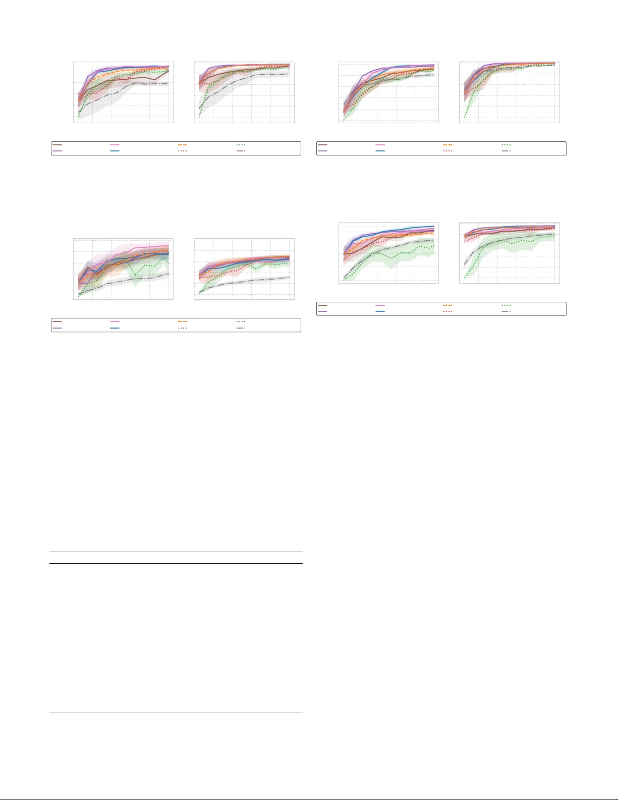
Acti v e In-Conte xt Learning for T ab ular F oundation Models W ilailuck T reerath and F abrizio Pittorino Dipartimento di Elettronica, Informazione e Bioingegneria, Politecnico di Milano, Milano, Italy Email: fabrizio.pittorino@polimi.it Abstract —Active learning (AL) reduces labeling cost by query- ing informati ve samples, b ut in tabular settings its cold-start gains ar e often limited because uncertainty estimates are un- reliable when models ar e trained on very few labels. T abular foundation models such as T abPFN provide calibrated proba- bilistic predictions via in-context learning (ICL), i.e., without task-specific weight updates, enabling an AL regime in which the labeled context - rather than parameters - is iteratively optimized. W e formalize T abular Active In-Context Learning (T ab-AICL) and instantiate it with four acquisition rules: un- certainty (T abPFN-Margin), diversity (T abPFN-Coreset), an un- certainty–diversity hybrid (T abPFN-Hybrid), and a scalable two- stage method (T abPFN-Proxy-Hybrid) that shortlists candidates using a lightweight linear proxy befor e T abPFN-based selection. Across 20 classification benchmarks, T ab-AICL impr oves cold- start sample efficiency ov er r etrained gradient-boosting baselines (CatBoost-Margin and XGBoost-Margin), measured by normal- ized A ULC up to 100 labeled samples. Index T erms —Active Lear ning, T abular Data, F oundation Models, In-Context Learning, T abPFN, Cold-Start. I . I N T RO D U C T I O N Activ e learning (AL) aims to reduce annotation cost by selecting informativ e samples to label [1], [2]. In tabular classification, howe ver , AL often provides limited benefit in the cold-start regime because acquisition functions depend on predictiv e uncertainty , which is unstable when models are fit on very small labeled sets. T abular foundation models such as T abPFN [3], [4] provide strong probabilistic predictions via in-context learning (ICL), i.e., without task-specific gradient-based training. This changes the AL perspectiv e: instead of repeatedly re-training a model after each query , we can treat the labeled set as a context that is iteratively refined to improv e predictions. Y et, using ICL inside an AL loop raises two practical issues. First, T abPFN inference scales quadratically with context length, making pool-wide scoring expensi ve for lar ge unlabeled sets. Second, uncertainty-based querying can be brittle on noisy or imbalanced pools, where high uncertainty may correspond to outliers rather than informativ e boundary points. W e propose T ab ular Active In-Conte xt Learning (T ab- AICL) , a framew ork that instantiates common acquisition principles within T abPFN-based ICL. W e consider four acqui- sition rules: uncertainty sampling (T abPFN-Margin), div ersity sampling (T abPFN-Coreset), an uncertainty–diversity hybrid (T abPFN-Hybrid), and a scalable two-stage v ariant (T abPFN- Proxy-Hybrid) that shortlists candidates with a lightweight logistic-regression proxy before T abPFN-based selection. W e ev aluate T ab-AICL on 20 tabular classification bench- marks with 10 random seeds, focusing on cold-start perfor- mance up to 100 labeled samples. Across datasets, T ab-AICL improv es normalized area under the learning curve (A ULC) ov er strong retrained baselines with fixed hyperparameters (CatBoost-Margin and XGBoost-Margin) on a majority of tasks. Consistent with the div ersity of tabular data regimes, no single acquisition rule dominates: margin sampling is strong on clean/structured datasets, hybrid selection often helps on clustered geometries, and proxy-hybrid is more robust when uncertainty sampling tends to fixate on outliers. I I . B A C K G RO U N D A N D R E L AT E D W O R K a) T abular Deep Learning and F oundation Models: Despite major advances of deep learning in vision and lan- guage, supervised learning on tabular data is still commonly addressed with tree-based ensembles [5], [6]. A recurring difficulty is that tab ular datasets combine heterogeneous fea- ture types and often operate in moderate-data regimes, where generic neural architectures can be less competitive without careful inductive bias and tuning [7], [8]. T abular foundation models such as T abPFN [3], [4] take a dif ferent route: a T ransformer is pretrained on large collections of synthetic tabular tasks and then applied to a new dataset via in-context learning, producing probabilistic predictions without task- specific gradient-based training. This makes T abPFN particu- larly relev ant for cold-start regimes, where reliable probability estimates are critical for downstream decision-making. b) Active Learning Challenges: Classical AL selects queries using acquisition functions deriv ed from model predic- tions, most commonly uncertainty-based criteria such as least confidence, mar gin, or entropy [1]. An alternative is di versity- or geometry-driv en selection, such as core-set (greedy k - center) methods [9], which aim to cover the input space but may under-sample informative boundary regions when class structure is complex. A large body of work in deep AL addresses the uncertainty–div ersity trade-off with batch-a ware objectiv es (e.g., BatchB ALD [10] and B ADGE [11]), often at substantial computational cost. c) F oundation Models and Active Learning: Recent work has begun exploring AL with foundation models in vision and language, where pretrained representations improve acquisition-function quality [12]–[14]. In the tabular domain, this intersection remains largely unexplored: T abPFN has been benchmarked as a predictor [3], [4] but not systematically stud- ied within an AL loop. Our work fills this gap by formalizing the AL-ICL coupling in the tabular foundation model context and providing a controlled empirical comparison. Our work sits at the intersection of these lines: we study AL when the predictor is an in-context tabular foundation model. Rather than introducing a new Bayesian batch objecti ve, we instantiate lightweight uncertainty , div ersity , and hybrid acquisitions within T abPFN inference, and add a simple proxy- based shortlist to reduce pool-scoring cost in practice. I I I . T A B U L A R A C T I V E I N - C O N T E X T L E A R N I N G T ab-AICL instantiates AL with an in-context tabular foun- dation model: the predictor is fix ed, and learning proceeds by expanding the labeled context given at inference time. The activ e loop selects which labeled examples to acquire and add to the context, rather than updating model parameters. A. Pr oblem F ormulation Let U = { x 1 , . . . , x M } denote an unlabeled pool and L 0 a small labeled set. At iteration t , an acquisition rule selects a batch Q t ⊂ U of size B to be labeled by an oracle. The labeled context is updated as L t +1 = L t ∪ { ( x, y ) : x ∈ Q t } , and queried points are removed from the pool. Gi ven a fixed model M capable of in-context learning (T abPFN), the objectiv e is to maximize predictive performance on a held-out test set as a function of the labeling budget |L t | . B. Data Prepr ocessing W e apply a single preprocessing pipeline Φ( · ) to all meth- ods. Features are treated as categorical or numerical using dataset metadata; if metadata are unav ailable, integer-v alued features with less than 20 unique values are treated as cate- gorical. Numerical features are mean-imputed (computed on the training pool) and standardized with StandardScaler . Categorical features are mode-imputed and encoded with OrdinalEncoder . All preprocessing parameters are fit on the training pool only (before querying) and then applied to both U and the test set to av oid leakage. The feature counts in T able I refer to the dimensionality after preprocessing. C. Acquisition Strate gies W e consider four acquisition rules that emphasize (i) uncer- tainty , (ii) diversity , or (iii) their combination under computa- tional constraints. 1) Margin Sampling ( T abPFN-Margin ): Margin sampling prioritizes points for which the model is least confident among its top predictions. Gi ven a probabilistic predictor M condi- tioned on conte xt L , let p k ( x ) = P ( ˆ y = k | x, L ) denote the predicted class probabilities and let p (1) ( x ) ≥ p (2) ( x ) ≥ · · · be these probabilities sorted in descending order . The margin score is α margin ( x ) = p (1) ( x ) − p (2) ( x ) , and we query the B points with smallest α margin ( x ) . Algorithm 1 T ab-AICL Margin Sampling ( T abPFN-Margin ) Require: Unlabeled pool U , labeled context L , batch size B , model M , budget N max 1: while |L| < N max and |U | > 0 do 2: P ← M . predict_proba ( U ; L ) 3: for each x i ∈ U compute α i ← p (1) ( x i ) − p (2) ( x i ) from P i 4: Q ← arg sort ( α )[: min( B , |U | )] // smallest mar gins 5: obtain labels for Q and update L ← L ∪ Oracle ( Q ) 6: update U ← U \ Q 7: end while 2) Hybrid Sampling ( T abPFN-Hybrid ): Hybrid sampling combines an uncertainty filter with a div ersity step. The intu- ition is to (i) restrict attention to a candidate set that the current predictor finds ambiguous, and then (ii) select a geometrically div erse batch from that candidate set. Concretely , we compute predictiv e entropy H ( x ) = − P K k =1 p k ( x ) log p k ( x ) , with p k ( x ) = P ( ˆ y = k | x, L ) , retain the N cand most entropic points, and run k -means ( k = B ) on their preprocessed feature vectors. W e then query the point nearest to each centroid. Algorithm 2 T ab-AICL Hybrid Sampling ( T abPFN-Hybrid ) Require: Unlabeled pool U , labeled context L , batch size B , model M , budget N max 1: while |L| < N max and |U | > 0 do 2: P ← M . predict_proba ( U ; L ) 3: for each x i ∈ U compute H i ← − P K k =1 p ik log( p ik + ε ) 4: N cand ← min  |U | , max(2 B , ⌊|U | / 2 ⌋ )  5: S ← topk ( H , N cand ) // highest entr opy indices 6: X ← { x i : i ∈ S } // in pr eprocessed feature space 7: fit k -means with k = B on X (if | X | < B , k ← | X | ) 8: Q ← nearest point to each centroid (unique selection; break ties arbitrarily) 9: obtain labels for Q and update L ← L ∪ Oracle ( Q ) 10: update U ← U \ Q 11: end while 3) Pr oxy-Hybrid Sampling ( T abPFN-Proxy-Hybrid ): The Proxy-Hybrid strategy reduces acquisition cost by screening the pool with a lightweight proxy and in voking T abPFN only on a shortlisted subset. At each iteration, we (i) fit a linear classifier P on the current labeled conte xt L , (ii) rank all x ∈ U by the proxy predictiv e entropy , and (iii) retain the top N proxy candidates, where N proxy is clamped to bound runtime: N proxy = min  |U | , max  N min , min( N max , α |U | )   , (1) with N min = 200 , N max = 2000 , and α = 0 . 05 in our experiments. W e then ev aluate T abPFN uncertainty only on this shortlist and apply a div ersity step to form the batch. W e use entropy for both stages. For a distribution p ( · | x ) , define H ( x ) = − P K k =1 p k ( x ) log( p k ( x ) + ε ) with ε > 0 . Let S short = topk ( H P , N proxy ) be the proxy shortlist. W e compute Algorithm 3 T ab-AICL Proxy-Hybrid Sampling ( T abPFN- Proxy-Hybrid ) Require: Unlabeled pool U , labeled context L , batch size B , model M , proxy P , b udget N max , filter ratio α , clamps ( N min , N proxy max ) 1: while |L| < N max and |U | > 0 do 2: fit proxy P on L 3: compute proxy entropy H P ( x ) for all x ∈ U 4: N proxy ← min  |U | , max  N min , min( N proxy max , ⌊ α |U |⌋ )   5: S short ← topk ( H P , N proxy ) 6: compute T abPFN entropy H M ( x ) for x ∈ S short using context L 7: N div ← min(3 B , |S short | ) 8: S final ← topk ( H M , N div ) 9: run k -means with k = min( B , |S final | ) on { x i : i ∈ S final } 10: Q ← nearest point to each centroid (unique selection; break ties arbitrarily) 11: update L ← L ∪ Oracle ( Q ) , U ← U \ Q 12: end while T abPFN entropy on S short , retain the N div = min(3 B , |S short | ) highest-entropy points, and run k -means with k = B on their preprocessed features. The queried batch Q contains the nearest point to each centroid (with unique selection). Pr oxy configuration and cost: In T abPFN-Proxy-Hybrid, the proxy P is a logistic regression classifier with balanced class weights. At each acquisition step, P scores all x ∈ U and we retain a shortlist S short containing the top α fraction of points by proxy predicti ve entropy ( α = 0 . 05 in our e xper- iments), subject to the clamping in (1). T abPFN uncertainty and the subsequent di versity step are computed only on S short , reducing the number of expensi ve T abPFN pool ev aluations by approximately a factor 1 /α . 4) Coreset Sampling (Diversity): W e adopt a greedy k - center (coreset) rule that promotes cov erage of the input space by selecting points that are far from the current labeled set in the standardized feature space. Let z ( · ) denote the preprocessing map and d ( · , · ) the Euclidean distance. At each selection, we pick x ∗ = arg max u ∈U min l ∈L ∥ z ( u ) − z ( l ) ∥ 2 , and repeat this procedure B times to form the query batch. T o av oid storing the full |U | × |L| distance matrix, we maintain a vector of current nearest-neighbor distances D min ( u ) = min l ∈L ∥ z ( u ) − z ( l ) ∥ 2 for all u ∈ U and update it incre- mentally after each ne wly selected point. This yields O ( |U | ) memory , with per-step time dominated by computing distances from the new center to all remaining unlabeled points. I V . E X P E R I M E N TA L S E T U P A. Active Learning Pr otocol W e simulate pool-based batch AL under a fixed labeling budget. For each dataset, we create a stratified 70/30 split into an unlabeled training pool U and a held-out test set, which is never used for acquisition or preprocessing decisions. Algorithm 4 T ab-AICL Coreset (Greedy k -Center) ( T abPFN- Coreset ) Require: Unlabeled pool U , labeled context L , batch size B , budget N max Ensure: Updated labeled context L 1: while |L| < N max do 2: // Maintain near est-labeled distance for each u ∈ U 3: D min ( u ) ← min l ∈L ∥ z ( u ) − z ( l ) ∥ 2 ∀ u ∈ U 4: Q ← ∅ 5: for j ← 1 to B do 6: q ← arg max u ∈U D min ( u ) 7: Q ← Q ∪ { q } 8: // Update distances after adding new center q 9: for all u ∈ U \ { q } do 10: D min ( u ) ← min( D min ( u ) , ∥ z ( u ) − z ( q ) ∥ 2 ) 11: end for 12: U ← U \ { q } 13: end for 14: L ← L ∪ Oracle ( Q ) 15: end while The initial labeled context L 0 contains one randomly sampled instance per class. At each round, an acquisition rule selects a batch Q t ⊂ U of size B without replacement, an oracle re veals the labels, and we update L t +1 = L t ∪ { ( x, y ) : x ∈ Q t } and U ← U \ Q t . The loop terminates when |L t | = N max = 100 . For very small datasets, we additionally stop once 50% of the original unlabeled pool is queried. B. Experimental Design and Evaluation W e repeat the full pipeline for 10 random seeds, resampling both the split and the initialization, and report mean ± std. W e ev aluate batch sizes B ∈ { 5 , 10 , 15 , 20 } to probe the trade-off between update frequenc y and within-batch diversity . T o com- pare the cold-start efficiency of different methodologies, we report the normalized area under the learning curve (A ULC) up to N max as the primary metric. Let y t denote the test-set Cohen κ after round t , when |L t | = n t . W e compute A ULC norm = 1 N max − n 0 T X t =1 y t + y t − 1 2 ( n t − n t − 1 ) , (2) which corresponds to the average κ over the cold-start acquisi- tion trajectory . W e also report final κ at N max and R OC A UC; for multi-class problems, R OC A UC is computed one-vs-rest with macro-a veraging. For significance testing, we use paired W ilcoxon signed-rank tests on per-seed AULC norm scores. T o control multiplicity across datasets, we apply Benjamini- Hochberg FDR correction and consider differences significant with the BH-adjusted p -value p adj < 0 . 05 . C. Baselines and Repr oducibility All methods are ev aluated within the same AL proto- col (identical splits, initialization L 0 , budget, and query- without-replacement). For T abPFN-based methods, we use T abPFN ( tabpfn Python package v6.2.0) with n estimators = 32 throughout. W e report four T ab-AICL acquisition rules (T abPFN-Margin, T abPFN-Coreset, T abPFN-Hybrid, T abPFN- Proxy-Hybrid) and a passive T abPFN-Random baseline that uses the same T abPFN configuration but selects Q t uniformly at random. The oracle is simulated: ground-truth labels from the dataset are rev ealed upon query . As retrained baselines, we include CatBoost and XGBoost with margin-based querying, where the model is refit from scratch at each round on the current labeled set L t . T o avoid per-dataset tuning, which would be impractical under a realis- tic cold-start protocol, we fix hyperparameters for stability in low-data regimes. n estimators = 2000 , learning rate = 0 . 05 , max depth = 6 , and early stopping rounds = 50 . W e use scikit-learn for preprocessing and logistic regression, and the official catboost and xgboost packages. Finally , we include a semi-supervised Label Spreading baseline [15] with a kNN kernel ( k = 7 ) and clamping factor α = 0 . 2 , paired with random acquisition to isolate the effect of the learner from the query rule. D. Datasets W e benchmark 20 classification datasets from OpenML [16] and UCI [17] (T able I), spanning heterogeneous domains and mixed feature types. T o keep runtime comparable across benchmarks and reflect practical labeling budgets, datasets with more than 10,000 instances are uniformly subsampled to 10,000 prior to splitting. All datasets are processed with the standardized pipeline described in Section III, and the reported feature counts correspond to the post-preprocessing dimensionality . T ABLE I B E NC H M A RK D A TA SE T S ( P O S T - P R EP R OC E S SI N G ) . Dataset ID Instances Features Classes Domain Iris 61 150 4 3 Botan y Glass 41 214 9 6 Forensic Ionosphere 59 351 34 2 Physics Balance-scale 997 625 4 2 Psychology V ehicle 994 846 18 2 Image Rec. Page-blocks 1021 5,473 10 2 Document Parkinsons 1488 195 22 2 Medicine Seeds 1499 210 7 3 Agriculture Bank-Marketing 45065 45,211 (sub: 10,000) 16 2 Finance Adult 45068 48,842 (sub: 10,000) 14 2 Social Sci. CoverT ype 1596 581,012 (sub: 10,000) 54 7 Forestry KC1 1066 145 94 2 Software JM1 46979 10,885 (sub: 10,000) 21 2 Software Blood-Transfusion 46913 748 4 2 Medicine Diabetes 46921 768 8 2 Medicine Tic-T ac-T oe 137 39,366 (sub: 10,000) 9 2 Game Theory Credit-g 46918 1,000 20 2 Finance Steel-Plates 46959 1,941 26 7 Industry Phoneme 44127 3,172 5 2 Speech Ilpd 41943 583 10 2 Medicine Datasets with more than 10,000 instances are subsampled uniformly to 10,000 prior to splitting. V . R E S U LT S A N D D I S C U S S I O N A. Cold-start efficiency vs. baselines T able II reports normalized A ULC up to 100 labels. In this regime, T abPFN provides a strong cold-start baseline and, when combined with active acquisition, attains the best A ULC on 15/20 datasets. Overall, T abPFN-based methods outperform the retrained GBDT baselines on 18/20 datasets, suggesting that ICL inference provides a fav orable inductive bias in the low-label setting. Nev ertheless, active querying is not uniformly beneficial: on Glass , Bank-Marketing , and Tic-Tac-Toe , T abPFN-Random matches or exceeds the ac- tiv e rules. Con versely , CatBoost-Margin remains competitiv e on KC1 and Ilpd , indicating that tree-based biases can still be effecti ve for some tabular datasets even under tight label budgets. For completeness, we report the corresponding final- step performance at the 100-label budget (Cohen’ s κ and R OC A UC) in Appendix A. W e test whether T abPFN-Hybrid impro ves o ver the strongest retrained GBDT baseline (CatBoost-Margin) using a paired W ilcoxon signed-rank test across seeds ( N seeds = 10 ) on normalized A ULC scores. T able III reports per -dataset differences ∆ A ULC and the corresponding p -values after Benjamini–Hochberg correction ov er the 20 datasets. After correction, T abPFN-Hybrid is significantly better on 8/20 datasets ( p adj < 0 . 05 ). In the opposite direction, CatBoost- Margin does not achieve a statistically significant advantage ov er T abPFN-Hybrid on any dataset under the same protocol. Across datasets, the benefit of acti ve querying is not uniform and no single acquisition rule is consistently best. T abPFN- Margin is frequently competitiv e, while adding a diversity step (T abPFN-Hybrid) can improve performance on some benchmarks. T abPFN-Proxy-Hybrid is often among the more stable options, but it does not dominate. Finally , on sev eral datasets T abPFN-Random matches or exceeds the activ e rules in the 0–100 label regime, indicating that acquisition can be dataset-sensitiv e under this budget and protocol. B. V isual analysis of learning trajectories Figures 1–5 complement the table results by showing how methods behave across the acquisition horizon. Fig. 1 summarizes the distribution of normalized A ULC across the 20 datasets: hybrid rules tend to be more consistent across datasets, while pure uncertainty sampling can be more variable depending on the pool. Inspection of representativ e learning curv es highlights recur- ring patterns. On structured datasets such as Ionosphere (Fig. 2), T abPFN-based methods typically reach high per- formance with fe wer queried labels than retrained GBDT baselines in the N < 50 regime. On noisier benchmarks such as Adult (Fig. 3), T abPFN-Pr oxy-Hybrid often exhibits tighter across-seed variability than uncertainty-only selection, consistent with the proxy stage reducing sensitivity to atypical points. On datasets with clustered or geometric structure, TabPFN-Hybrid frequently maintains strong performance throughout the curve (e.g., Vehicle , Fig. 4), suggesting that combining an uncertainty filter with a simple diversity step can be beneficial. Finally , some acquisition rules show early differences that narro w as the labeled set grows, indicating that advantages are concentrated in the cold-start region rather than at the final budget. Overall, the figures suggest that differences between acquisition rules are driven not only by T ABLE II AU L C P E R FO R M A NC E S U M MA RY ( M E AN ± S T D O F AU L C U P T O N = 100 , B A T C H S I Z E 1 0 ) Dataset T ab-AICL Strategies Baselines T abPFN-Coreset T abPFN-Hybrid T abPFN-Proxy-Hybrid T abPFN-Margin T abPFN-Random CatBoost-Margin XGBoost-Margin LabelSpreading-Random Iris 0.934 ± 0.023 0.929 ± 0.029 0.931 ± 0.019 0.917 ± 0.027 0.902 ± 0.031 0.880 ± 0.060 0.743 ± 0.074 0.831 ± 0.058 Glass 0.397 ± 0.055 0.472 ± 0.041 0.441 ± 0.061 0.481 ± 0.056 0.489 ± 0.077 0.456 ± 0.055 0.400 ± 0.033 0.382 ± 0.061 Ionosphere 0.617 ± 0.132 0.810 ± 0.042 0.800 ± 0.032 0.788 ± 0.038 0.751 ± 0.052 0.641 ± 0.051 0.640 ± 0.049 0.440 ± 0.154 Balance-scale 0.758 ± 0.032 0.808 ± 0.024 0.811 ± 0.040 0.808 ± 0.044 0.721 ± 0.055 0.609 ± 0.042 0.578 ± 0.058 0.665 ± 0.049 V ehicle 0.742 ± 0.067 0.833 ± 0.022 0.811 ± 0.054 0.794 ± 0.040 0.747 ± 0.052 0.665 ± 0.057 0.640 ± 0.062 0.685 ± 0.056 Page-blocks 0.602 ± 0.064 0.687 ± 0.044 0.657 ± 0.043 0.704 ± 0.023 0.624 ± 0.042 0.592 ± 0.038 0.349 ± 0.166 0.430 ± 0.044 Parkinsons 0.575 ± 0.126 0.629 ± 0.125 0.618 ± 0.128 0.580 ± 0.160 0.580 ± 0.125 0.574 ± 0.135 0.489 ± 0.127 0.520 ± 0.089 Seeds 0.891 ± 0.030 0.907 ± 0.014 0.903 ± 0.022 0.900 ± 0.026 0.893 ± 0.037 0.839 ± 0.047 0.742 ± 0.030 0.841 ± 0.041 Bank-Marketing 0.211 ± 0.074 0.175 ± 0.077 0.217 ± 0.100 0.158 ± 0.043 0.258 ± 0.075 0.148 ± 0.058 0.150 ± 0.060 0.091 ± 0.025 Adult 0.298 ± 0.077 0.292 ± 0.059 0.358 ± 0.067 0.317 ± 0.079 0.300 ± 0.099 0.307 ± 0.060 0.236 ± 0.065 0.131 ± 0.038 CoverT ype 0.349 ± 0.042 0.383 ± 0.029 0.315 ± 0.046 0.378 ± 0.049 0.378 ± 0.025 0.326 ± 0.046 0.302 ± 0.035 0.188 ± 0.017 KC1 0.356 ± 0.100 0.391 ± 0.084 0.412 ± 0.103 0.378 ± 0.121 0.377 ± 0.128 0.417 ± 0.130 0.391 ± 0.090 0.281 ± 0.093 JM1 0.105 ± 0.059 0.137 ± 0.028 0.106 ± 0.056 0.069 ± 0.071 0.090 ± 0.061 0.080 ± 0.053 0.049 ± 0.037 0.088 ± 0.046 Blood-Transfusion 0.143 ± 0.086 0.126 ± 0.059 0.126 ± 0.093 0.151 ± 0.101 0.109 ± 0.085 0.148 ± 0.072 0.091 ± 0.068 0.140 ± 0.063 Diabetes 0.340 ± 0.046 0.392 ± 0.051 0.401 ± 0.069 0.362 ± 0.053 0.379 ± 0.050 0.344 ± 0.062 0.288 ± 0.057 0.192 ± 0.077 Tic-T ac-T oe 0.071 ± 0.042 0.145 ± 0.053 0.175 ± 0.075 0.142 ± 0.099 0.189 ± 0.041 0.122 ± 0.068 0.128 ± 0.079 0.076 ± 0.028 Credit-g 0.163 ± 0.056 0.180 ± 0.070 0.164 ± 0.058 0.146 ± 0.065 0.116 ± 0.060 0.159 ± 0.082 0.075 ± 0.054 0.105 ± 0.049 Steel-Plates 0.323 ± 0.039 0.484 ± 0.018 0.350 ± 0.079 0.450 ± 0.037 0.435 ± 0.036 0.419 ± 0.042 0.342 ± 0.032 0.367 ± 0.031 Phoneme 0.417 ± 0.053 0.476 ± 0.053 0.440 ± 0.122 0.444 ± 0.083 0.475 ± 0.055 0.416 ± 0.047 0.372 ± 0.063 0.417 ± 0.051 Ilpd 0.065 ± 0.072 0.089 ± 0.057 0.109 ± 0.087 0.115 ± 0.069 0.111 ± 0.068 0.147 ± 0.053 0.112 ± 0.048 0.100 ± 0.060 Note: Bold indicates the strategy with the highest mean A ULC per dataset. All values represent Mean ± Standard Deviation across 10 random seeds. T ABLE III S T A T IS T I C AL S I G N IFI C A NC E : T AB P F N -H Y B RI D V S . C AT B O O S T - M A RG I N ( W IL C OX O N S I G N ED - R A NK T E S T O N AU LC ) Dataset ∆ A ULC p -V alue (Raw) p -V alue (Adj) Result Iris +0.050 0.037 0.080 No significant difference Glass +0.016 0.375 0.526 No significant difference Ionosphere +0.169 0.002 0.007 Significantly higher Balance-scale +0.199 0.002 0.007 Significantly higher V ehicle +0.168 0.002 0.007 Significantly higher Page-blocks +0.095 0.002 0.007 Significantly higher Parkinsons +0.054 0.375 0.526 No significant difference Seeds +0.068 0.004 0.012 Significantly higher Bank-Marketing +0.028 0.557 0.683 No significant difference Adult -0.015 0.695 0.789 No significant difference CoverT ype +0.057 0.002 0.007 Significantly higher KC1 -0.027 0.492 0.635 No significant difference JM1 +0.057 0.004 0.012 Significantly higher Blood-Transfusion -0.023 0.375 0.526 No significant difference Diabetes +0.048 0.037 0.080 No significant difference Tic-T ac-T oe +0.023 0.557 0.683 No significant difference Credit-g +0.020 0.557 0.683 No significant difference Steel-Plates +0.064 0.004 0.012 Significantly higher Phoneme +0.060 0.084 0.161 No significant difference Ilpd -0.058 0.131 0.229 No significant difference Note: ∆ AULC is the mean difference in AULC . The Result column is determined by the Benjamini-Hochberg corrected p -value ( p ad j < 0 . 05 ). p ad j indicates Benjamini-Hochberg (FDR) corrected v alues . final performance but by how quickly and how stably they improv e during the 0 – 100 label regime. C. Computational efficiency analysis T abPFN-based acquisition can be expensiv e because scor- ing candidates requires repeated in-context inference, whose attention cost grows quadratically with the context size. The proposed T abPFN-Proxy-Hybrid reduces the dominant cost by restricting T abPFN scoring to a proxy-defined shortlist. Concretely , a logistic-regression proxy computes uncertainty ov er the full pool and we retain only an α = 0 . 05 fraction (clamped as described in Section 3); T abPFN then ev aluates uncertainty and performs diversity selection only within this subset. Relati ve to scoring all of U with T abPFN, this reduces the number of T abPFN ev aluations by approximately a factor 1 /α (about 20 × when the clamp is inactiv e). T ab-AICL (Hybrid) T ab-AICL (Proxy-Hybrid) T ab-AICL (Margin) T ab-AICL (Random) T ab-AICL (Coreset) CatBoost (Margin) XGBoost (Margin) LabelSpreading (Random) 0.0 0.1 0.2 0.3 0.4 0.5 Mean Cohen's Kappa AULC 0.467 (±0.030) 0.457 (±0.042) 0.454 (±0.040) 0.446 (±0.039) 0.418 (±0.039) 0.414 (±0.039) 0.356 (±0.040) 0.348 (±0.035) Average Cohen's Kappa AULC across Datasets (95% CI) Fig. 1. Comprehensive A ULC Performance: Area Under Learning Curve scores across 20 datasets, grouped by acquisition strategy . Batch size influences runtime through two opposing effects: smaller batches increase the number of acquisition iterations, while larger batches increase the context size and the cost of each T abPFN call. In our implementation, intermediate values (e.g., B = 10 ) provide a practical compromise. D. Ablation study: batch size W e study the ef fect of the query batch size B on cold- start efficienc y by running the same AL protocol with B ∈ { 5 , 10 , 15 , 20 } (T able IV). As expected, smaller batches can improv e normalized A ULC because the context is updated more frequently , allowing the model to re vise its predic- tions after fewer newly labeled points. At the same time, performance is reasonably stable across batch sizes on most datasets, with only modest degradation as B increases. This suggests that T ab-AICL can be used with larger batches – often preferred in practice to amortize annotation overhead – without materially changing the main conclusions. V I . L I M I TA T I O N S , T R A D E - O FF S , A N D C O N C L U S I O N T ab-AICL reframes active learning for tabular foundation models as context optimization : at each step, we update the 0 20 40 60 80 100 Labeled Samples 0.0 0.2 0.4 0.6 0.8 Cohen's Kappa Ionosphere - Cohen's Kappa (95% CI) 0 20 40 60 80 100 Labeled Samples 0.5 0.6 0.7 0.8 0.9 1.0 ROC AUC Ionosphere - ROC AUC (95% CI) T ab-AICL (Coreset) T ab-AICL (Hybrid) T ab-AICL (Proxy-Hybrid) T ab-AICL (Margin) T ab-AICL (Random) CatBoost (Margin) XGBoost (Margin) LabelSpreading (Random) Fig. 2. Learning Curve for Ionosphere: T ab-AICL strategies achieve rapid con ver gence, with T abPFN-Proxy-Hybrid offering an effecti ve balance of speed and stability . The shaded regions represent 95% confidence intervals across 10 random seeds. 0 20 40 60 80 100 Labeled Samples 0.0 0.1 0.2 0.3 0.4 0.5 Cohen's Kappa Adult - Cohen's Kappa (95% CI) 0 20 40 60 80 100 Labeled Samples 0.5 0.6 0.7 0.8 0.9 1.0 ROC AUC Adult - ROC AUC (95% CI) T ab-AICL (Coreset) T ab-AICL (Hybrid) T ab-AICL (Proxy-Hybrid) T ab-AICL (Margin) T ab-AICL (Random) CatBoost (Margin) XGBoost (Margin) LabelSpreading (Random) Fig. 3. Learning Curve for Adult: The T abPFN-Proxy-Hybrid strategy (pink) demonstrates stable performance and consistent gains. Note the narrower confidence intervals compared to other strategies. labeled conte xt pro vided to T abPFN rather than retraining task- specific parameters. Across 20 classification benchmarks (10 seeds), T abPFN-based methods are strong cold-start predictors, and in many cases acti ve acquisition improves normalized A ULC up to 100 labels relativ e to both random querying and retrained gradient-boosting baselines under the same protocol. Howe ver , the results also show clear trade-offs and regime dependence. T ABLE IV B ATC H S I Z E A B L A T I ON ( AU L C ± S T D , T A B PF N - P ROX Y - H Y BR I D ) Dataset B=5 B=10 B=15 B=20 Iris 0.920 ± 0.036 0.931 ± 0.019 0.910 ± 0.016 0.907 ± 0.022 Glass 0.446 ± 0.059 0.441 ± 0.061 0.467 ± 0.040 0.442 ± 0.027 Ionosphere 0.809 ± 0.044 0.800 ± 0.032 0.784 ± 0.049 0.766 ± 0.092 Balance-scale 0.836 ± 0.038 0.811 ± 0.040 0.791 ± 0.037 0.772 ± 0.044 V ehicle 0.837 ± 0.040 0.811 ± 0.054 0.817 ± 0.040 0.776 ± 0.054 Page-blocks 0.651 ± 0.075 0.657 ± 0.043 0.623 ± 0.069 0.632 ± 0.059 Parkinsons 0.620 ± 0.114 0.618 ± 0.128 0.621 ± 0.113 0.625 ± 0.144 Seeds 0.911 ± 0.023 0.903 ± 0.022 0.900 ± 0.023 0.901 ± 0.024 Bank-Marketing 0.209 ± 0.056 0.217 ± 0.100 0.220 ± 0.086 0.188 ± 0.082 Adult 0.356 ± 0.076 0.358 ± 0.067 0.348 ± 0.061 0.340 ± 0.061 CoverT ype 0.341 ± 0.032 0.315 ± 0.046 0.329 ± 0.045 0.324 ± 0.049 KC1 0.393 ± 0.098 0.412 ± 0.103 0.377 ± 0.122 0.326 ± 0.114 JM1 0.085 ± 0.039 0.106 ± 0.056 0.097 ± 0.064 0.112 ± 0.041 Blood-Transfusion 0.107 ± 0.059 0.126 ± 0.093 0.109 ± 0.086 0.107 ± 0.087 Diabetes 0.387 ± 0.064 0.401 ± 0.069 0.368 ± 0.081 0.366 ± 0.071 Tic-T ac-T oe 0.158 ± 0.083 0.175 ± 0.075 0.175 ± 0.080 0.158 ± 0.088 Credit-g 0.132 ± 0.057 0.164 ± 0.058 0.102 ± 0.078 0.145 ± 0.049 Steel-Plates 0.371 ± 0.067 0.350 ± 0.079 0.373 ± 0.061 0.379 ± 0.046 Phoneme 0.449 ± 0.076 0.440 ± 0.122 0.390 ± 0.160 0.417 ± 0.147 Ilpd 0.107 ± 0.091 0.109 ± 0.087 0.131 ± 0.070 0.104 ± 0.080 Remark: Experiments conducted with fixed Proxy Filter α = 0 . 05 . 0 20 40 60 80 100 Labeled Samples 0.0 0.2 0.4 0.6 0.8 1.0 Cohen's Kappa V ehicle - Cohen's Kappa (95% CI) 0 20 40 60 80 100 Labeled Samples 0.5 0.6 0.7 0.8 0.9 1.0 ROC AUC V ehicle - ROC AUC (95% CI) T ab-AICL (Coreset) T ab-AICL (Hybrid) T ab-AICL (Proxy-Hybrid) T ab-AICL (Margin) T ab-AICL (Random) CatBoost (Margin) XGBoost (Margin) LabelSpreading (Random) Fig. 4. Learning Curve for V ehicle: The T abPFN-Hybrid strategy (purple) achiev es higher performance than pure uncertainty sampling and baselines. 0 20 40 60 80 100 Labeled Samples 0.0 0.2 0.4 0.6 0.8 Cohen's Kappa Page-blocks - Cohen's Kappa (95% CI) 0 20 40 60 80 100 Labeled Samples 0.5 0.6 0.7 0.8 0.9 1.0 ROC AUC Page-blocks - ROC AUC (95% CI) T ab-AICL (Coreset) T ab-AICL (Hybrid) T ab-AICL (Proxy-Hybrid) T ab-AICL (Margin) T ab-AICL (Random) CatBoost (Margin) XGBoost (Margin) LabelSpreading (Random) Fig. 5. Learning Curve for Page Blocks: The T abPFN-Margin strategy (blue) achiev es rapid con vergence, suggesting that for certain data manifolds, pure uncertainty sampling remains an effecti ve approach. a) Limitations and trade-offs: First, T ab-AICL is inher- ently a small-data approach: inference scales quadratically with the conte xt length and is bounded by the model maximum context window , so benefits can saturate as the labeled set grows and costs increase. Second, the very early phase remains sensitiv e to initialization: with only a fe w labeled points, class imbalance or unlucky seeds can bias the trajectory before acquisition rules hav e enough signal to correct it. Third, acquisition rules can fail in predictable ways. Uncertainty- based selection can over -focus on atypical or noisy points; div ersity-only selection can waste labels away from infor - mativ e regions; and proxy filtering introduces an additional modeling assumption that may be lossy on complex tasks. b) Practical implication: These constraints suggest using T ab-AICL as a cold-start module : exploit T abPFN (optionally with activ e acquisition) to rapidly reach a competent model with tens to a few hundred labels, then hand off to scalable tabular learners (e.g., CatBoost/XGBoost) when additional labels are av ailable and retraining costs become acceptable. c) Future dir ections: T wo concrete extensions follow naturally: (i) automatic criteria that decide when to transi- tion from context-based inference to retrained models, and (ii) context compression/distillation methods that transfer the information in the acquired context into a lightweight student, mitigating the quadratic inference cost. Meta-selection of acquisition rules could also be designed, using early iterations to choose between uncertainty-, diversity-, and proxy-based strategies rather than committing to a single rule a priori. T ABLE V F I NA L K A P P A P E R F OR M A N CE S U M M ARY ( M E AN ± S T D AT N = 100 , B A T C H S I Z E 1 0 ) Dataset T ab-AICL Strategies Baselines T abPFN-Coreset T abPFN-Hybrid T abPFN-Proxy-Hybrid T abPFN-Margin T abPFN-Random CatBoost-Margin XGBoost-Margin LabelSpreading-Random Iris 0.950 ± 0.043 0.933 ± 0.049 0.950 ± 0.037 0.943 ± 0.047 0.947 ± 0.034 0.927 ± 0.047 0.880 ± 0.092 0.877 ± 0.060 Glass 0.564 ± 0.053 0.580 ± 0.060 0.585 ± 0.061 0.637 ± 0.055 0.592 ± 0.094 0.588 ± 0.091 0.496 ± 0.024 0.441 ± 0.066 Ionosphere 0.805 ± 0.078 0.875 ± 0.039 0.888 ± 0.044 0.878 ± 0.034 0.860 ± 0.037 0.821 ± 0.047 0.800 ± 0.065 0.574 ± 0.069 Balance Scale 0.871 ± 0.033 0.918 ± 0.029 0.940 ± 0.024 0.949 ± 0.018 0.885 ± 0.034 0.742 ± 0.050 0.756 ± 0.065 0.762 ± 0.035 V ehicle 0.916 ± 0.070 0.966 ± 0.022 0.980 ± 0.014 0.989 ± 0.009 0.921 ± 0.065 0.929 ± 0.018 0.897 ± 0.024 0.810 ± 0.053 Page Blocks 0.744 ± 0.039 0.732 ± 0.039 0.775 ± 0.056 0.807 ± 0.026 0.693 ± 0.048 0.751 ± 0.042 0.519 ± 0.181 0.597 ± 0.059 Parkinsons 0.692 ± 0.099 0.731 ± 0.141 0.767 ± 0.115 0.772 ± 0.102 0.677 ± 0.161 0.716 ± 0.129 0.703 ± 0.134 0.626 ± 0.102 Seeds 0.921 ± 0.037 0.936 ± 0.024 0.931 ± 0.031 0.926 ± 0.029 0.921 ± 0.035 0.879 ± 0.052 0.852 ± 0.040 0.869 ± 0.034 Bank-Marketing 0.308 ± 0.116 0.235 ± 0.105 0.280 ± 0.114 0.216 ± 0.079 0.322 ± 0.062 0.208 ± 0.055 0.150 ± 0.112 0.094 ± 0.032 Adult 0.388 ± 0.083 0.377 ± 0.072 0.455 ± 0.056 0.378 ± 0.090 0.408 ± 0.074 0.408 ± 0.069 0.297 ± 0.160 0.205 ± 0.050 Covertype 0.439 ± 0.027 0.445 ± 0.024 0.381 ± 0.049 0.471 ± 0.018 0.447 ± 0.029 0.420 ± 0.039 0.388 ± 0.038 0.240 ± 0.028 KC1 0.435 ± 0.113 0.482 ± 0.120 0.455 ± 0.100 0.447 ± 0.132 0.423 ± 0.234 0.508 ± 0.132 0.292 ± 0.188 0.389 ± 0.116 JM1 0.075 ± 0.050 0.151 ± 0.046 0.119 ± 0.059 0.061 ± 0.070 0.076 ± 0.056 0.080 ± 0.060 0.044 ± 0.054 0.097 ± 0.056 Blood-Transfusion 0.127 ± 0.107 0.161 ± 0.082 0.205 ± 0.103 0.197 ± 0.100 0.114 ± 0.086 0.212 ± 0.114 0.151 ± 0.122 0.143 ± 0.063 Diabetes 0.434 ± 0.042 0.447 ± 0.062 0.454 ± 0.058 0.417 ± 0.048 0.429 ± 0.051 0.372 ± 0.061 0.290 ± 0.149 0.242 ± 0.090 Tic-T ac-T oe 0.090 ± 0.098 0.189 ± 0.056 0.203 ± 0.065 0.181 ± 0.098 0.233 ± 0.109 0.180 ± 0.079 0.163 ± 0.107 0.111 ± 0.049 Credit-g 0.229 ± 0.096 0.261 ± 0.073 0.251 ± 0.070 0.236 ± 0.079 0.209 ± 0.104 0.225 ± 0.071 0.122 ± 0.113 0.156 ± 0.049 Steel-Plates 0.451 ± 0.068 0.617 ± 0.019 0.411 ± 0.108 0.592 ± 0.030 0.574 ± 0.034 0.510 ± 0.037 0.465 ± 0.042 0.468 ± 0.040 Phoneme 0.517 ± 0.055 0.563 ± 0.040 0.555 ± 0.091 0.607 ± 0.028 0.588 ± 0.029 0.578 ± 0.037 0.456 ± 0.096 0.496 ± 0.051 Ilpd 0.023 ± 0.041 0.086 ± 0.099 0.133 ± 0.106 0.096 ± 0.058 0.185 ± 0.104 0.156 ± 0.059 0.093 ± 0.095 0.134 ± 0.075 Note: Bold indicates the strategy with the highest mean Kappa per dataset. All values represent Mean ± Standard Deviation across 10 random seeds. T ABLE VI F I NA L RO C AU C P E R F OR M A N CE S U M M ARY ( M E AN ± S T D AT N = 100 , B A T C H S I Z E 1 0 ) Dataset T ab-AICL Strategies Baselines T abPFN-Coreset T abPFN-Hybrid T abPFN-Proxy-Hybrid T abPFN-Margin T abPFN-Random CatBoost-Margin XGBoost-Margin LabelSpreading-Random Iris 0.997 ± 0.003 0.995 ± 0.005 0.996 ± 0.003 0.996 ± 0.004 0.996 ± 0.004 0.994 ± 0.006 0.956 ± 0.044 0.986 ± 0.009 Glass 0.921 ± 0.026 0.929 ± 0.018 0.926 ± 0.016 0.936 ± 0.013 0.929 ± 0.033 0.907 ± 0.022 0.849 ± 0.017 0.854 ± 0.041 Ionosphere 0.973 ± 0.009 0.984 ± 0.007 0.985 ± 0.006 0.987 ± 0.006 0.981 ± 0.008 0.964 ± 0.016 0.947 ± 0.018 0.899 ± 0.044 Balance Scale 0.989 ± 0.003 0.994 ± 0.003 0.996 ± 0.002 0.998 ± 0.002 0.990 ± 0.006 0.956 ± 0.012 0.955 ± 0.030 0.957 ± 0.011 V ehicle 0.996 ± 0.003 0.999 ± 0.001 1.000 ± 0.000 1.000 ± 0.000 0.998 ± 0.001 0.995 ± 0.003 0.986 ± 0.008 0.975 ± 0.011 Page Blocks 0.962 ± 0.011 0.977 ± 0.006 0.964 ± 0.022 0.968 ± 0.025 0.968 ± 0.012 0.952 ± 0.024 0.874 ± 0.064 0.900 ± 0.030 Parkinsons 0.932 ± 0.055 0.958 ± 0.040 0.940 ± 0.077 0.956 ± 0.035 0.919 ± 0.053 0.935 ± 0.036 0.925 ± 0.047 0.916 ± 0.036 Seeds 0.996 ± 0.003 0.995 ± 0.003 0.996 ± 0.003 0.996 ± 0.003 0.995 ± 0.004 0.982 ± 0.009 0.975 ± 0.014 0.986 ± 0.005 Bank-Marketing 0.836 ± 0.033 0.837 ± 0.025 0.830 ± 0.036 0.799 ± 0.057 0.854 ± 0.011 0.759 ± 0.047 0.705 ± 0.062 0.655 ± 0.031 Adult 0.841 ± 0.024 0.820 ± 0.042 0.833 ± 0.030 0.830 ± 0.051 0.851 ± 0.027 0.817 ± 0.023 0.778 ± 0.056 0.658 ± 0.033 Covertype 0.904 ± 0.011 0.898 ± 0.008 0.886 ± 0.014 0.902 ± 0.008 0.899 ± 0.009 0.841 ± 0.010 0.786 ± 0.017 0.761 ± 0.028 KC1 0.817 ± 0.071 0.812 ± 0.041 0.824 ± 0.055 0.816 ± 0.039 0.814 ± 0.094 0.827 ± 0.046 0.798 ± 0.046 0.801 ± 0.044 JM1 0.643 ± 0.076 0.673 ± 0.027 0.645 ± 0.034 0.638 ± 0.075 0.670 ± 0.035 0.626 ± 0.041 0.621 ± 0.057 0.537 ± 0.039 Blood-Transfusion 0.717 ± 0.058 0.721 ± 0.045 0.720 ± 0.030 0.705 ± 0.047 0.697 ± 0.046 0.656 ± 0.049 0.660 ± 0.044 0.609 ± 0.027 Diabetes 0.819 ± 0.018 0.827 ± 0.021 0.820 ± 0.017 0.814 ± 0.020 0.819 ± 0.020 0.761 ± 0.042 0.730 ± 0.048 0.723 ± 0.036 Tic-T ac-T oe 0.680 ± 0.027 0.681 ± 0.038 0.668 ± 0.033 0.651 ± 0.068 0.722 ± 0.023 0.648 ± 0.042 0.638 ± 0.045 0.602 ± 0.029 Credit-g 0.712 ± 0.030 0.752 ± 0.027 0.746 ± 0.021 0.724 ± 0.024 0.743 ± 0.031 0.679 ± 0.051 0.645 ± 0.043 0.648 ± 0.040 Steel-Plates 0.889 ± 0.019 0.906 ± 0.017 0.891 ± 0.015 0.906 ± 0.024 0.900 ± 0.024 0.884 ± 0.015 0.846 ± 0.029 0.855 ± 0.024 Phoneme 0.829 ± 0.024 0.849 ± 0.020 0.826 ± 0.030 0.864 ± 0.014 0.865 ± 0.013 0.842 ± 0.018 0.816 ± 0.026 0.810 ± 0.019 Ilpd 0.727 ± 0.025 0.718 ± 0.032 0.704 ± 0.037 0.676 ± 0.052 0.729 ± 0.021 0.661 ± 0.054 0.636 ± 0.061 0.633 ± 0.026 Note: Bold indicates the strategy with the highest mean R OC A UC per dataset. All values represent Mean ± Standard Deviation across 10 random seeds. While this work focuses on classification, future research should extend T ab-AICL to regression and multi-label tabular problems, adapting the acquisition functions and potentially dev eloping specialized foundation models for these tasks. A C K N O W L E D G M E N T S This paper is supported by PNRR-PE-AI F AIR project funded by the NextGeneration EU program. A P P E N D I X A F I NA L - S T E P M E T R I C S A T T H E 1 0 0 - L A B E L B U D G E T W e report final-step performance at the b udget limit ( |L| = 100 ) for all methods, using Cohen’ s κ (T able V) and ROC A UC (one-vs-rest macro-a verage for multi-class; T able VI), complementing the normalized A ULC results in the main text. R E F E R E N C E S [1] B. Settles, “ Active learning literature survey , ” 2009. [Online]. A vailable: http://digital.library .wisc.edu/1793/60660 [2] P . Ren, Y . Xiao, X. Chang, P .-Y . Huang, Z. Li, B. B. Gupta, X. Chen, and X. W ang, “ A survey of deep active learning, ” New Y ork, NY , USA, Oct. 2021. [Online]. A vailable: https://doi.org/10.1145/3472291 [3] N. Hollmann, S. M ¨ uller , K. Eggensperger , and F . Hutter, “T abPFN: A transformer that solves small tabular classification problems in a second, ” 2022. [Online]. A vailable: https://openreview .net/forum?id= eu9fVjV asr4 [4] N. Hollmann, S. M ¨ uller , L. Purucker, A. Krishnakumar, M. K ¨ orfer , S. Hoo, R. Schirrmeister, and F . Hutter, “ Accurate predictions on small data with a tabular foundation model, ” Nature , v ol. 637, pp. 319–326, 01 2025. [5] V . Borisov , T . Leemann, K. Seßler, J. Haug, M. Pawelczyk, and G. Kasneci, “Deep neural networks and tabular data: A survey , ” IEEE T ransactions on Neural Networks and Learning Systems , vol. 35, no. 6, pp. 7499–7519, 2024. [6] R. Shwartz-Ziv and A. Armon, “T abular data: Deep learning is not all you need, ” pp. 84–90, 2022. [Online]. A vailable: https://www .sciencedirect.com/science/article/pii/S1566253521002360 [7] Y . Gorishniy , I. Rubachev , V . Khrulko v , and A. Babenko, “Revisiting deep learning models for tabular data, ” Red Hook, NY , USA, 2021. [8] J. P . Gardner, Z. Popovi, and L. Schmidt, “Subgroup robustness grows on trees: An empirical baseline in vestigation, ” in Advances in Neural Information Processing Systems , A. H. Oh, A. Agarwal, D. Belgrave, and K. Cho, Eds., 2022. [Online]. A vailable: https: //openrevie w .net/forum?id=6QvmtRjWNRy [9] O. Sener and S. Sav arese, “ Active learning for con volutional neural networks: A core-set approach, ” 2018. [Online]. A vailable: https://openrevie w .net/forum?id=H1aIuk- R W [10] A. Kirsch, J. van Amersfoort, and Y . Gal, “Batchbald: Efficient and diverse batch acquisition for deep bayesian active learning, ” in Advances in Neural Information Processing Systems , H. W allach, H. Larochelle, A. Beygelzimer , F . d'Alch ´ e-Buc, E. Fox, and R. Garnett, Eds., vol. 32. Curran Associates, Inc., 2019. [Online]. A vailable: https://proceedings.neurips.cc/paper files/paper/ 2019/file/95323660ed2124450caaac2c46b5ed90- Paper .pdf [11] J. T . Ash, C. Zhang, A. Krishnamurthy , J. Langford, and A. Agarwal, “Deep batch activ e learning by diverse, uncertain gradient lower bounds, ” in International Conference on Learning Representations , 2020. [Online]. A vailable: https: //openrevie w .net/forum?id=ryghZJBKPS [12] T . W an, K. Xu, T . Y u, X. W ang, D. Feng, B. Ding, and H. W ang, “ A survey of deep activ e learning for foundation models, ” Intelligent Computing , vol. 2, p. 0058, 2023. [Online]. A vailable: https://spj.science.org/doi/abs/10.34133/icomputing.0058 [13] K. Margatina, T . Schick, N. Aletras, and J. Dwivedi-Y u, “ Active learning principles for in-context learning with large language models, ” in F indings of the Association for Computational Linguistics: EMNLP 2023 , H. Bouamor , J. Pino, and K. Bali, Eds. Singapore: Association for Computational Linguistics, Dec. 2023, pp. 5011–5034. [Online]. A vailable: https://aclanthology .org/2023.findings- emnlp.334/ [14] G. Citovsky , G. DeSalvo, C. Gentile, L. Karydas, A. Rajagopalan, A. Rostamizadeh, and S. Kumar , “Batch activ e learning at scale, ” in Advances in Neural Information Processing Systems , A. Beygelzimer , Y . Dauphin, P . Liang, and J. W . V aughan, Eds., 2021. [Online]. A vailable: https://openreview .net/forum?id=zzdf0CirJM4 [15] D. Zhou, O. Bousquet, T . Lal, J. W eston, and B. Sch ¨ olkopf, “Learning with local and global consistency , ” in Advances in Neural Information Pr ocessing Systems , S. Thrun, L. Saul, and B. Sch ¨ olkopf, Eds., vol. 16. MIT Press, 2003. [Online]. A vailable: https://proceedings.neurips.cc/paper files/paper/ 2003/file/87682805257e619d49b8e0dfdc14aff a- Paper .pdf [16] J. V anschoren, J. N. van Rijn, B. Bischl, and L. T orgo, “Openml: networked science in machine learning, ” SIGKDD Explor . Newsl. , vol. 15, no. 2, p. 49–60, Jun. 2014. [Online]. A vailable: https: //doi.org/10.1145/2641190.2641198 [17] D. Dua and C. Gra, “Uci machine learning repository , ” 2017. [Online]. A vailable: http://archive.ics.uci.edu/ml