Unsupervised Evaluation of Deep Audio Embeddings for Music Structure Analysis

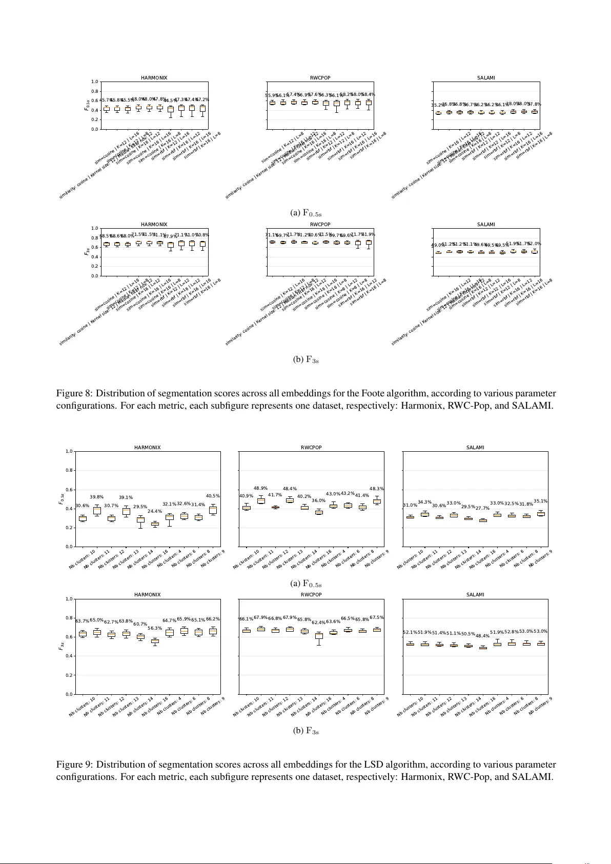
U N S U P E RV I S E D E V A L UA T I O N O F D E E P A U D I O E M B E D D I N G S F O R M U S I C S T R U C T U R E A N A LY S I S Axel M A R M O R E T (axel.marmoret@imt-atlantique.fr) (0000-0001-6928-7490) 1 1 BRAIN team, MEE , IMT Atlantique , Brest, France ABSTRA CT Music Structure Analysis (MSA) aims to uncover the high- lev el organization of musical pieces. State-of-the-art meth- ods are often based on supervised deep learning, but these methods are bottlenecked by the need for hea vily anno- tated data and inherent structural ambiguities. In this pa- per , we propose an unsupervised e valuation of nine open- source, generic pre-trained deep audio models, on MSA. For each model, we extract barwise embeddings and seg- ment them using three unsupervised segmentation algo- rithms (Foote’ s checkerboard kernels, spectral clustering, and Correlation Block-Matching (CBM)), focusing exclu- siv ely on boundary retrie val. Our results demonstrate that modern, generic deep embeddings generally outperform traditional spectrogram-based baselines, b ut not systemati- cally . Furthermore, our unsupervised boundary estimation methodology generally yields stronger performance than recent linear probing baselines. Among the ev aluated tech- niques, the CBM algorithm consistently emerges as the most effecti ve downstream segmentation method. Finally , we highlight the artificial inflation of standard ev aluation metrics and advocate for the systematic adoption of “trim- ming”, or e ven “double trimming” annotations to establish more rigorous MSA ev aluation standards. 1. INTR ODUCTION Beyond just sound, music is an intricate organization of scales and rhythms. At its core, musical composition re- lies on repetition, contrast, and v ariation to or ganize sound into coherent forms. These elements create an internal logic that dictates a song’ s shape, establishing recognizable sections separated by distinct transitions. Music Structure Analysis (MSA) is the task of identifying this high-lev el organization. Specifically , it aims to partition a musical piece into meaningful, non-ov erlapping sections ( e.g . , in- tro, verse, chorus, or bridge), and in particular locating their precise temporal boundaries [1]. Be yond its estab- lished v alue in guiding applications like music summariza- tion, cover song identification, and data-dri ven musicol- ogy , we believe that MSA will find renewed significance in the era of generativ e AI. By providing a structural frame- work, accurate MSA can enhance the editability , user con- trol, and long-term coherence of AI-generated audio [2, 3]. Copyright: © 2026. This is an open-access article distrib uted under the terms of the Creative Commons Attribution 3.0 Unported License , which permits unre- stricted use, distribution, and repr oduction in any medium, pro vided the original author and source are credited. Y et, despite its practical importance, MSA remains a no- toriously challenging task: musical form is inherently hi- erarchical, and multiple structural interpretations can be simultaneously valid depending on the listener’ s focus, the annotation protocol, and the desired le vel of granular- ity . Early work on MSA focused on self-similarity ma- trices (SSMs) [1, 4], i.e. square matrices indicating the pairwise similarity of all time instances in a song. From this viewpoint, sections are often understood as large, ho- mogeneous and/or repeating regions, and boundaries as salient ruptures between subsequent sections. Compar- ing time instances to detect change points was the root of MSA for years, with significant research in the previ- ous decade dedicated to refining the similarity computa- tion between these instances [5–7]. This line of work was significantly advanced by the rise of deep learning, particu- larly representation learning [8–11]. Researchers have be- gun to use deep models in conjunction with standard down- stream self-similarity segmentation algorithms to improve audio understanding. For instance, Salamon et al. [9] used deep embeddings to replace the traditional acoustic fea- tures in [6], improving the performance. Parallel to these de velopments, supervised deep learn- ing models [12–14] emerged as a dominant approach, ex- plicitly learning to predict boundaries from labeled data and achieving state-of-the-art performance in MSA. How- ev er , this success comes with significant trade-of fs. Super - vised models rely hea vily on large, meticulously annotated datasets, which are time-consuming and costly to produce. Furthermore, the inherent ambiguity of musical structure becomes a major bottleneck here: supervised training of- ten forces the model to bias its estimates tow ards a single “ground truth” annotation protocol. This effecti vely dis- cards other potentially v alid, equi v alent structural interpre- tations and limits the model’ s ability to generalize across different musical distrib utions. Recent Self-Supervised Learning (SSL) paradigms offer a promising path to alleviate these issues. By lev eraging pretext tasks (such as Masked Acoustic Modeling, where random masks are applied to segments of the input sig- nal and the model is optimized to reconstruct the corrupted regions), these networks bypass the annotation bottleneck and learn directly from massi ve, unlabeled audio corpora. SSL dedicated to MSA has been shown to be effecti ve in recent work [11]. Ho wev er , an intriguing open question remains: do broad, general-purpose audio representations naturally encode structure-related information as a byprod- uct of their pre-training, even without being explicitly de- signed for structure? T o succeed in their pre-training tasks, these generic SSL models must intrinsically capture the underlying structural, timbral, and temporal characteristics of acoustic signals. Recent work by T oyama et al. [15] ex- plored whether generic deep audio models (SSL-based b ut not only) could benefit MSA. Howe ver , their study ev alu- ated learned representations using linear probing, which in volv es training a supervised linear head on top of the frozen embeddings to estimate structure. While compu- tationally ef ficient, linear probing remains fundamentally supervised. Consequently , it remains sensitiv e to the man- ual biases that limit fully supervised models. Our work shares the fundamental premise of T oyama et al. [15], b ut we employ strictly unsuper- vised downstream segmentation. In this paper , we study unsupervised boundary estimation using frozen embeddings extracted from nine open-source, generic, pre-trained audio models [16–24]. Follo wing our previous work [7], these embeddings are computed at the bar scale. W e ev aluate these embeddings by computing barwise SSMs, and segment them using three standard and state- of-the-art unsupervised segmentation algorithms: Foote’ s checkerboard kernels [4], spectral clustering (LSD) [6], and the Correlation Block-Matching (CBM) algorithm [7]. W e focus on the boundary retrie val task only , and do not attempt to label the sections. Our goal is two-fold: on one hand, to assess to what extent modern deep audio embed- dings are rich enough to provide structured information about the data, and in turn improv e unsupervised MSA; on the other hand, to compare the potential of traditional unsupervised segmentation algorithms to be improved when complemented with deep representation learning. The remainder of this paper details our methodology for extracting and segmenting barwise embeddings (Sec- tion 2), outlines the experimental setup and ev aluation met- rics (Section 3), discusses our comparativ e results (Sec- tion 4), and concludes (Section 5). 2. METHODOLOGY 2.1 Deep Audio Models T o ev aluate the structural information captured by modern representation learning, we extract embeddings from nine distinct open-source deep audio models [16–24]. These deep audio models differ significantly in their architec- tures and training objectiv es. Three of these nine mod- els (MER T [17], MusicFM [18], and MuQ [19]) are only trained on music data, and their respectiv e authors explic- itly noted their potential utility for MSA. The majority of the e valuated architectures rely on Masked Acoustic Modeling, an SSL paradigm where the network optimizes the reconstruction of masked portions of the audio signal. Within this category , AudioMAE [16] learns by reconstructing masked spectrogram patches. Meanwhile, MER T [17], MusicFM [18], and MuQ [19] learn to reconstruct indirect representations of the au- dio. Specifically , MER T uses pseudo-labels from acous- tic teacher models, MusicFM predicts targets via a ran- dom projection quantizer , and MuQ predicts discrete to- kens generated by a single-layer Residual V ector Quantiza- tion (R VQ). Additionally , M2D [20] and MA TP A C++ [21] employ Masked Latent Prediction, using two models: one computing latent features of masked patches, the other one estimating these latent features from visible patches. MA T - P A C++ further incorporates Multiple Choice Learning to model prediction ambiguity , which could turn out to be very rele v ant for tackling the inherent ambiguity of MSA. A second category of ev aluated models consists of Neu- ral Audio Codecs, which are generally designed as au- toencoders to compress audio as aggressively as possi- ble while maintaining high reconstruction fidelity . The extreme compression bottleneck forces these networks to learn highly abstract and compact latent representations of the acoustic space. DA C [22] is a prominent example of this approach, operating as a CNN-based autoencoder that utilizes R VQ to compress audio into discrete hierarchical tokens. T o address the codebook collapse sometimes asso- ciated with traditional R VQ, CoDiCodec [23] utilizes Fi- nite Scalar Quantization (FSQ) to project continuous rep- resentations onto a fixed integer grid. This architecture al- lows CoDiCodec to simultaneously extract both continu- ous summary embeddings and discrete acoustic tokens. Finally , the study explores models utilizing cross-modal contrastiv e learning, a paradigm aimed at bridging acous- tic features with human-interpretable semantic concepts by aligning audio and text latent spaces. CLAP [24] is the only ev aluated model not pretrained via SSL re- construction objectives; its core audio encoder was orig- inally trained for supervised audio classification before be- ing aligned with text in a shared multimodal space, using contrastiv e learning. Furthermore, while M2D [20] and MuQ [19] primarily focus on acoustic reconstruction, the y also incorporate this contrastiv e learning approach. Conse- quently , these specific frame works yield tw o distinct repre- sentations: a unimodal audio space and a joint multimodal representation. 2.2 Barwise Processing In the context of W estern modern music, we adopt the bar-scale as a musically motiv ated temporal resolution for MSA. Musical form is fundamentally tied to this met- rical hierarchy , as macroscopic structural changes and repetitions frequently align with bar boundaries. Be- yond this musical intuition, the validity of do wnbeat- synchronized boundaries is supported empirically: our previous work [7] demonstrated that barwise alignment maintains or impro ves the performance of F oote’ s checker- board kernels [4] and CBM [7] algorithms, when compared with beat-scale processing. In that sense, embeddings will be indi vidually computed on the different bars of the sig- nal, thus resulting in barwise embeddings. 2.3 Downstr eam Segmentation Algorithm After the computation of barwise deep embeddings, we ap- ply three state-of-the-art unsupervised algorithms to per- form the boundary retriev al task. All of these algorithms are based on SSMs 1 . Foote’ s algorithm [4] is a nov elty- 1 Authors of [6] prefer to mention “affinity matrices”, with a clear def- inition of their computation, but the main principle remains the same. based method that identifies abrupt structural transitions by correlating a square checkerboard kernel along the main diagonal of the SSM. Conv ersely , the LSD approach [6] takes a graph-theoretic perspective to capture long-term repetitions; it treats the SSM as an adjacency matrix and analyzes the eigen vectors of its normalized Laplacian to estimate boundaries via K-means change-points. Finally , the CBM algorithm [7] frames boundary retrie val as a global optimization problem solv ed via dynamic program- ming. Conceptually similar to Foote’ s method but op- timized for detecting homogeneous regions rather than abrupt nov elty , CBM identifies optimal boundaries by maximizing a score function that represents block struc- tures around the main diagonal. 3. EXPERIMENT AL SETTINGS 3.1 Implementation Details W e operate entirely at the bar scale, estimating downbeats using the Beat This! [25] model. T o ensure compatibil- ity , ra w audio signals are segmented into bar -length chunks before computing embeddings from each model’ s final la- tent layer . Because the ev aluated models operate at differ- ent nativ e temporal resolutions, we homogenize the rep- resentations by av eraging across the temporal dimension, yielding a single vector per bar . W e adopt this frame- work for consistency , despite the contradiction between the gains reported in [15] and the temporal preservation fa vored by [7]. In vestigating this specific impact is be yond our current scope. Using these barwise embeddings, we compute barwise SSMs via both RBF and Cosine similarity measures, then segmented using Foote’ s and CBM algorithms. The ex- ception is the LSD algorithm, which inherently computes its own specialized affinity matrix to emphasize diagonal stripes. W e also ev aluate Barwise TF matrices [7], which will represent our baseline non-deep learning condition, and are constructed by flattening intra-bar time-frequency information. T o ensure optimal and fair do wnstream performance, we performed a comprehensive grid search ov er the hyperparameters of each segmentation algorithm. For Foote’ s algorithm, we searched both the kernel size and the novelty curve median filtering over the set { 8 , 12 , 16 } . For LSD, we varied the number of clusters 𝑘 ∈ { 4 , 6 , 8 , 9 , 10 , 11 , 12 , 13 , 14 , 16 } 2 and set the me- dian filtering parameter equal to 𝑘 3 . F or the CBM al- gorithm, we compared the Full and 7-band kernels. Cru- cially , we disabled the CBM penalty function that en- forces specific segment sizes; omitting this penalty lim- its empirical structural priors and ensures the resulting segmentation better reflects the discriminativ e power of the e valuated embeddings. A study of the influence of these hyperparameters is presented in the Appendix. LSD and Foote are computed using the MSAF [26] toolbox, and the CBM using the original implementation. Re- 2 W e observe a high variability of the results giv en this parameter; de- tailed results are av ailable in the Appendix. 3 W e found this beneficial in preliminary experiments using Optuna. garding the deep learning models, we used HuggingF ace for pretrained deep learning models whenev er possible ( i.e. for AudioMAE, CLAP , D A C, MER T , and MuQ), re- spectiv ely using the checkpoints hance-ai/audiomae , laion/clap-htsat-unfused , descript/dac 44khz , MERT-v1-95M , and MuQ | MuQ-MuLan-large (for audio and multimodal spaces). All other pre-trained models, de- veloped in pytorc h [27], were downloaded from their of- ficial repositories: CoDiCodec 4 , M2D 5 , MA TP A C++ 6 , and MusicFM 7 (MSD checkpoint). W e release our code for reproducing experiments 8 . 3.2 Metrics & Datasets Follo wing standard protocols, we assess boundary detec- tion using the hit-rate F-measure at 0.5s and 3s tolerances ( F 0 . 5s and F 3s respectiv ely). Scores are computed using mir eval [28]. W e handle data via mir data [29] and ev al- uate our approach on three standard MSA benchmarks: R WC-Pop [30] (no w open-source [31]), SALAMI [32], and Harmonix [33]. For R WC-Pop, we use the MIREX10 annotation set across its 100 popular music tracks. From the SALAMI dataset, we restrict our e valuation to the 884 tracks that possess two independent annotations as in [9, 14]; we ev aluate against the coarse-lev el annotations and report the best score among both annotations. Finally , we utilize the 912 W estern popular music tracks compris- ing the Harmonix set. 3.3 T rimming T rimming annotations and predictions consists of remov- ing the first and last segments before computing scores. While often overlook ed in the literature (to the best of our knowledge, only works of Buisson et al. [11, 14] systemat- ically trim annotations), e v aluating the impact of trimming is critical for a rigorous analysis: the absolute first and last boundaries does not provide insight into segmentation quality and can artificially inflate performance metrics. In our e xperiments, we will present results without trim- ming first, to remain consistent with existing literature. Nonetheless, we will also present comparative results of our best scores with and without trimming to study the ap- parent drop in performance that occurs when this artificial inflation is remov ed. When analyzing the R WC-Pop (MIREX10) and SALAMI datasets, we observed that annotations sys- tematically include silent segments at the file extremities (specifically , segments between 0 and the start of the audio signal, and between the end of the signal and the end of the file). W e argue that these segments do not provide meaningful information regarding the quality of a structural prediction and should therefore be excluded. W e term this preprocessing step “double trimming”: first, removing the silent segments, and subsequently trimming both annotations and predictions to the acti ve signal 4 https://github.com/SonyCSLParis/codicodec 5 https://github.com/nttcslab/m2d 6 https://github.com/aurianworld/matpac 7 https://github.com/minzwon/musicfm 8 https://github.com/ax- le/msa_deep_embeddings CBM F oote LSD 0.0 0.2 0.4 0.6 0.8 1.0 F 0 . 5 s 48.28% 46.95% 37.41% 55.30% 51.99% 44.63% HARMONIX CBM F oote LSD 58.51% 57.50% 48.17% 69.26% 63.27% 53.77% R WCPOP CBM F oote LSD 40.02% 36.96% 33.70% 44.04% 42.11% 38.34% S AL AMI * Hyperparameter are selected as the optimistic condition: * For each embedding-dataset pair, we select the best performance ( b e s t a v e r a g e o f F 0 . 5 s a n d F 3 s ) . Barwise TF featur es Best Deep (a) Best results obtained for F 0 . 5s CBM F oote LSD 0.0 0.2 0.4 0.6 0.8 1.0 F 3 s 68.84% 72.39% 65.21% 73.79% 73.71% 70.55% HARMONIX CBM F oote LSD 71.27% 71.41% 67.48% 82.13% 74.89% 71.10% R WCPOP CBM F oote LSD 55.98% 52.87% 52.51% 59.47% 56.26% 57.61% S AL AMI * Hyperparameter are selected as the optimistic condition: * For each embedding-dataset pair, we select the best performance ( b e s t a v e r a g e o f F 0 . 5 s a n d F 3 s ) . Barwise TF featur es Best Deep (b) Best results obtained for F 3s Figure 1: Comparison of the best results obtained with deep models and the Barwise TF features (non-deep learning baseline), according to the segmentation algorithm and the dataset. The hyperparameters of the downstream segmentation algorithms are selected as the best performing ones ( F 0 . 5s and F 3s av erage) per model and dataset. HARMONIX R WCPOP S AL AMI MA TP A C++ M2D - multimodal CoDiCodec - continuous M2D - audio space MuQ - audio space MER T CL AP CoDiCodec - discr ete Baseline (barwise TF) MusicFM MuQ - multimodal AudioMAE D A C 5 5 . 3 0 C 6 9 . 2 6 C 4 4 . 0 4 C 5 1 . 2 7 C 6 5 . 1 4 C 4 1 . 7 8 C 5 3 . 0 0 C 6 7 . 1 0 C 3 9 . 9 8 C 5 2 . 0 5 C 6 4 . 7 5 C 3 8 . 6 5 C 5 2 . 3 1 C 6 5 . 9 2 C 3 8 . 0 7 F 5 2 . 4 3 C 6 4 . 5 3 C 3 9 . 8 1 C 4 9 . 3 2 C 6 1 . 6 0 C 4 0 . 2 8 C 5 0 . 2 8 C 6 2 . 7 8 C 3 8 . 7 5 C 4 6 . 9 5 F 6 1 . 4 8 C 4 0 . 0 2 C 4 9 . 8 8 F 6 2 . 7 1 C 3 8 . 4 8 F 4 5 . 4 1 C 6 2 . 4 6 C 3 9 . 1 3 C 3 1 . 7 5 C 3 8 . 6 2 C 3 2 . 3 2 C 2 4 . 5 5 C 3 4 . 3 7 C 3 1 . 8 3 C F 0 . 5 s HARMONIX R WCPOP S AL AMI 7 3 . 7 9 C 8 2 . 1 3 C 5 9 . 4 7 C 7 1 . 1 4 C 8 0 . 7 9 C 5 8 . 2 7 C 7 2 . 6 4 C 8 0 . 3 4 C 5 5 . 3 0 C 7 0 . 4 8 C 7 9 . 0 0 C 5 3 . 6 5 C 7 1 . 0 4 C 7 8 . 1 7 C 5 2 . 3 6 F 7 0 . 1 1 C 7 7 . 1 4 C 5 3 . 3 1 C 6 9 . 2 3 C 7 7 . 8 4 C 5 6 . 6 9 C 7 0 . 7 4 C 7 8 . 0 4 C 5 4 . 3 0 C 7 2 . 3 9 F 7 6 . 1 4 C 5 5 . 9 8 C 7 2 . 2 3 F 7 5 . 4 5 C 5 2 . 5 2 F 6 7 . 9 4 C 7 9 . 3 4 C 5 5 . 7 7 C 5 6 . 9 2 C 5 9 . 6 3 C 4 4 . 6 2 C 4 7 . 6 9 C 5 4 . 4 3 C 4 3 . 3 4 C F 3 s 0.0 0.2 0.4 0.6 0.8 1.0 Scor e Figure 2: Best results obtained with all deep learning models, and their best do wnstream segmentation algorithm. Rows are ordered by decreasing av erage of F 0 . 5s and F 3s . Superscript denotes the downstream segmentation algorithm used to obtain these results ( 𝐶 : CBM, 𝐹 : Foote). The hyperparameters of the do wnstream segmentation algorithms are selected as the best performing ones ( F 0 . 5s and F 3s av erage) per model and dataset. boundaries. W e also ev aluate the impact of this condition on the resulting performance scores. Since the annotations for the Harmonix dataset do not systematically contain these silences, we remove them by default; consequently , trimming on Harmonix is de facto considered double trimming. Ideally , we expect that future standards in MSA will adopt trimming, or ev en double trimming, by default. 4. RESUL TS AND DISCUSSION 4.1 Deep Models vs. Barwise TF features Figure 1 compares peak deep audio models’ perfor- mance against the Barwise TF baseline. Deep em- beddings achie ve the highest scores across all datasets and algorithms, demonstrating clear improvements ov er spectrogram-based features. T able 1: Deep model segmentation performance across datasets (%), using the CBM algorithm as the do wnstream seg- mentation algorithm (shown to be the best one on average). Hyperparameters are selected as the best on av erage across all datasets, per model. Best results per column are highlighted in bold . ⋆ represents models where annotations were trimmed. † represents results where the dataset was used for training (in cross-v alidation settings). Deep Model HARMONIX R WCPOP SALAMI F 0 . 5 F 3 F 0 . 5 F 3 F 0 . 5 F 3 AudioMAE 31 . 75 ± 18.21 56 . 92 ± 18.46 38 . 62 ± 16.19 59 . 63 ± 18.01 25 . 86 ± 12.98 43 . 51 ± 15.76 CLAP 49 . 32 ± 21.38 69 . 23 ± 17.26 61 . 60 ± 17.98 77 . 84 ± 17.01 35 . 18 ± 16.70 51 . 72 ± 17.32 CoDiCodec Discrete 50 . 28 ± 20.52 70 . 74 ± 16.02 62 . 78 ± 16.98 78 . 04 ± 15.27 35 . 01 ± 16.74 50 . 51 ± 17.72 Continuous 53 . 00 ± 20.70 72 . 64 ± 16.34 67 . 10 ± 18.25 80 . 34 ± 15.11 36 . 54 ± 17.31 51 . 73 ± 17.55 D A C 24 . 10 ± 19.38 47 . 08 ± 21.57 34 . 37 ± 16.83 54 . 43 ± 19.45 25 . 59 ± 13.17 42 . 87 ± 15.71 M2D Audio space 52 . 05 ± 18.79 70 . 48 ± 14.30 65 . 14 ± 13.77 75 . 79 ± 12.70 36 . 02 ± 16.88 49 . 29 ± 17.95 Multimodal 50 . 90 ± 21.50 70 . 59 ± 17.22 65 . 14 ± 15.97 80 . 79 ± 15.42 36 . 10 ± 17.24 52 . 58 ± 17.71 MA TP A C++ 55 . 30 ± 20.83 73 . 79 ± 15.75 69 . 26 ± 16.42 82 . 13 ± 14.88 38 . 90 ± 17.66 53 . 74 ± 17.74 MER T 52 . 43 ± 19.25 70 . 11 ± 14.98 64 . 53 ± 15.41 77 . 14 ± 13.79 36 . 81 ± 16.80 49 . 52 ± 17.98 MuQ Audio space 51 . 97 ± 18.66 69 . 67 ± 14.62 65 . 92 ± 13.99 78 . 17 ± 13.06 35 . 68 ± 16.89 48 . 73 ± 17.70 Multimodal 45 . 41 ± 20.40 67 . 94 ± 17.27 62 . 46 ± 16.57 79 . 34 ± 14.93 33 . 95 ± 15.73 51 . 30 ± 16.97 MusicFM 51 . 55 ± 18.18 70 . 52 ± 13.86 59 . 66 ± 11.58 71 . 50 ± 11.35 38 . 37 ± 16.02 51 . 95 ± 16.88 Barwise TF baselines Foote 46 . 95 ± 19.18 72 . 39 ± 14.63 57 . 50 ± 13.70 71 . 41 ± 13.72 36 . 96 ± 15.67 52 . 87 ± 16.98 LSD 37 . 41 ± 16.07 65 . 21 ± 14.24 48 . 17 ± 12.73 67 . 48 ± 14.68 33 . 70 ± 12.61 52 . 51 ± 14.65 CBM 48 . 28 ± 17.56 68 . 84 ± 13.25 58 . 51 ± 12.60 71 . 27 ± 11.71 40 . 02 ± 14.76 55 . 98 ± 15.16 Literature results AudioMAE scores from [15] 36.95 58.11 - - - - CLAP scores from [15] 29.21 46.60 - - - - D A C scores from [15] 19.10 39.63 - - - - MER T scores from [15] 42.23 60.99 - - - - MusicFM scores from [15] 49.76 63.91 - - - - Salamon et al. [9] 45.74 68.84 - - 33.78 55.65 W ang et al. [10] 49.7 73.8 - - - - Buisson et al. (supervised) [14] ⋆ 56.8 † 71.7 † 58.5 † 75.0 † - - Buisson et al. (SSL) [11] ⋆ 48.5 80.8 - - 39.8 ± 16 70.1 ± 17 Figure 2 ranks the nine e valuated deep models. No- tably , three of them (and one multimodal space) are out- performed by the baseline. The fact that nearly a third of the models fail to beat traditional acoustic features sug- gests that their specific pretraining objectives or latent spaces may not align well with structural musical proper- ties. Among the successful models, MA TP A C++ achieves the highest overall performance with M2D and the continu- ous space of CoDiCodec closely following, indicating their latent spaces are particularly well-suited to disambiguate barwise audio representations. Although we observe dif- ferences when using multimodal versus unimodal audio spaces, the results are contradictory across conditions and yield no conclusiv e advantage for either approach. Both discrete embedding spaces (D A C and the discrete ver- sion of CoDiCodec) yielded relativ ely poor performance, with CoDiCodec’ s discrete representation notably under- performing its continuous counterpart. This suggests that discrete embeddings are ill-suited for our methodology . Fi- nally , models trained exclusi vely on music data (MER T , MusicFM, and MuQ) consistently underperform, with re- sults ranging from medium to poor . Overall, these results demonstrate that while the rich se- mantic and temporal contexts of learned representations provide a distinct advantage for boundary detection, off- the-shelf deep audio embeddings do not uni versally guar - antee improved segmentation over standard feature-based representations. T able 2: MA TP A C++ and Barwise TF-CBM results from T able 1, in different trimming conditions. Method HARMONIX R WCPOP SALAMI F 0 . 5 F 3 F 0 . 5 F 3 F 0 . 5 F 3 MA TP A C++ No trimming 55 . 30 ± 20.83 73 . 79 ± 15.75 69 . 26 ± 16.42 82 . 13 ± 14.88 38 . 90 ± 17.66 53 . 74 ± 17.74 T rimming − − 65 . 39 ± 18.48 79 . 87 ± 16.83 30 . 05 ± 19.51 47 . 12 ± 19.70 Double trimming 54 . 27 ± 23.35 70 . 96 ± 17.83 65 . 04 ± 21.67 77 . 88 ± 19.10 28 . 20 ± 22.21 43 . 33 ± 21.93 Barwise TF No trimming 48 . 28 ± 17.56 68 . 84 ± 13.25 58 . 51 ± 12.60 71 . 27 ± 11.71 40 . 02 ± 14.76 55 . 98 ± 15.16 CBM Trimming − − 53 . 18 ± 14.33 67 . 59 ± 13.26 28 . 80 ± 16.78 47 . 65 ± 17.98 Double trimming 45 . 55 ± 19.79 65 . 10 ± 15.14 51 . 00 ± 16.67 64 . 08 ± 15.09 25 . 68 ± 19.78 42 . 38 ± 21.67 4.2 Downstr eam Segmentation Algorithm As indicated by the results in Figure 2, CBM is the most effecti v e downstream segmentation algorithm for the vast majority of embedding-dataset pairs. Although the Foote algorithm occasionally achie ves superior performance (no- tably with CoDiCodec), CBM performs best in 33 out of 36 conditions. These results demonstrate the interest of the CBM in MSA, e ven in conjunction with deep embeddings. This study also marks the first application of the LSD al- gorithm at the bar scale. Unlike the Foote and CBM al- gorithms, designed to identify novelty and homogeneity ( i.e. abrupt changes or local similarity), LSD is specialized for detecting ”stripes” ( i.e. repeating patterns). Given its prov en effecti veness in the literature [11], we hypothesize that LSD’ s relative underperformance here stems from a misalignment with the barwise representations (a premise for barwise processing is a higher homogeneity between bars than beats) rather than a limitation of the algorithm itself to segment deep embeddings. 4.3 Results compared with literature Next, we compare our approach against state-of-the-art models in T able 1. For this comparison, we report results using only the CBM downstream algorithm, with hyper- parameters fixed to the best av erage configuration across all datasets for each model. This standardized setting mit- igates the optimistic bias of dataset-specific tuning, ensur- ing a fairer and more realistic comparison. Fiv e of the nine models (AudioMAE [16], Mu- sicFM [18], MER T [17], DA C [22], and CLAP [24]) were compared in [15], where their embeddings were studied in a linear probing fashion. Comparing our CBM-based downstream approach to these linear probing baselines on the Harmonix dataset, we observe that our methodology yields significantly stronger performance for almost all shared models. Most notably , CLAP and MER T sho w sub- stantial improvements, rising from 29.21% to 49.32% and from 42.23% to 52.43% for F 0 . 5s , respecti vely . This sug- gests that the CBM algorithm and barwise processing are highly ef fectiv e at extracting structural information from these deep audio embeddings, notably when compared with linear probing. These results validate our approach. In addition, we observe that MA TP A C++ prov es highly competitiv e with specialized literature on both Harmonix and R WC-Pop: it obtains the highest scores among our ev aluated embeddings, surpassed only by the two models from Buisson et al. [11, 14]. Overall, the self-supervised approach by Buisson et al. [11] achiev es the best results for F 3s by a wide margin, though its performance on F 0 . 5s is comparatively lower . W e conclude that while SSL representations ded- icated to MSA (with appropriate priors) offer significant benefits, there is still room for refinement. Specifically , we hypothesize that incorporating barwise processing could substantially improv e F 0 . 5s performance. Consequently , we conclude from these findings that developing future barwise SSL models, segmented using a standard se gmen- tation algorithm (notably the CBM algorithm), may im- prov e current results. 4.4 T rimming r esults Finally , we present trimmed results in T able 2. These re- sults demonstrate a consistent loss of performance when trimming annotations, which was expected. While trim- ming has only a mar ginal impact on the Harmonix dataset, the degradation can be sev ere elsewhere; for instance, F 0 . 5s performance drops by more than 11% points for the CBM on the SALAMI dataset, and degrades ev en further with double trimming. Because standard e valuation without trimming can artificially inflate scores by re warding tri vial boundary matches, we advocate that trimming should be adopted as the new standard for rigorous MSA e v aluation. 5. CONCLUSION In this work, we in vestigated the training-free capabili- ties of nine generic deep audio models for Music Struc- ture Analysis, specifically focusing on boundary retriev al. By leveraging unsupervised downstream segmentation al- gorithms at the bar scale, we demonstrated that deep au- dio embeddings generally provide a distinct advantage ov er traditional barwise acoustic features. Among the ev aluated representations, MA TP AC++ prov ed particularly well-suited for estimating structural boundaries. Further- more, our comparati ve analysis established the Correla- tion Block-Matching algorithm as the most highly effecti ve downstream segmentation method, notably outperforming recent linear probing approaches. Despite these advancements, the state-of-the-art model remains a self-supervised model specifically designed for Music Structure Analysis. Future research should thus fo- cus on dev eloping specialized SSL models, potentially at the bar scale, and using standard segmentation algorithms like the CBM. Additionally , we demonstrated that tradi- tional ev aluation metrics are often artificially inflated by initial and final boundary matches. W e strongly advocate for the community to adopt standard trimming and double trimming practices for more rigorous future ev aluations. 6. REFERENCES [1] O. Nieto et al. , “ Audio-based music structure analy- sis: Current trends, open challenges, and applications, ” T r ans. Int. Soc. for Music Information Retrieval , vol. 3, no. 1, 2020. [2] F . Morreale, M. A. Martinez-Ramirez, R. Masu, W . Liao, and Y . Mitsufuji, “Reductive, exclusionary , normalising: the limits of generative ai music, ” T r ans. Int. Soc. Music Information Retrieval , vol. 8, no. 1, 2025. [3] Y . Choi, J. Moon, J. Y oo, and J.-H. Hong, “Under- standing the potentials and limitations of prompt-based music generativ e ai, ” in Pr oceedings of the 2025 CHI Confer ence on Human F actors in Computing Systems , 2025. [4] J. Foote, “ Automatic audio segmentation using a mea- sure of audio nov elty , ” in 2000 IEEE Int. Conf. Multi- media and Expo. ICME2000. IEEE, 2000, pp. 452– 455. [5] J. Serr ` a, M. M ¨ uller , P . Grosche, and J. L. Arcos, “Un- supervised music structure annotation by time series structure features and se gment similarity , ” IEEE T rans. Multimedia , vol. 16, no. 5, pp. 1229–1240, 2014. [6] B. McFee and D. Ellis, “ Analyzing song structure with spectral clustering, ” in Int. Soc. Music Information Re- trieval Conf. (ISMIR) , 2014, pp. 405–410. [7] A. Marmoret, J. E. Cohen, and F . Bimbot, “Barwise music structure analysis with the correlation block- matching segmentation algorithm, ” T rans. Int. Soc. for Music Information Retrieval , vol. 6, no. 1, pp. 167– 185, 2023. [8] M. C. McCallum, “Unsupervised learning of deep fea- tures for music se gmentation, ” in 2019 IEEE Int. Conf. on Acoustics, Speech and Signal Pr ocessing (ICASSP) . IEEE, 2019, pp. 346–350. [9] J. Salamon, O. Nieto, and N. J. Bryan, “Deep embed- dings and section fusion improv e music se gmentation, ” in Int. Soc. Music Information Retrieval Conf. (ISMIR) , 2021. [10] J.-C. W ang, J. B. Smith, W .-T . Lu, and X. Song, “Su- pervised metric learning for music structure feature, ” in Int. Soc. Music Information Retrieval Conf. (ISMIR) , 2021, pp. 730–737. [11] M. Buisson, B. McFee, S. Essid, and H. C. Crayencour , “Self-supervised learning of multi-level audio repre- sentations for music segmentation, ” IEEE/ACM T rans. on Audio, Speech, and Languag e Processing , vol. 32, pp. 2141–2152, 2024. [12] T . Grill and J. Schl ¨ uter , “Music boundary detection us- ing neural networks on combined features and two- lev el annotations, ” in Int. Soc. Music Information Re- trieval Conf. (ISMIR) , 2015, pp. 531–537. [13] T . Kim and J. Nam, “ All-in-one metrical and func- tional structure analysis with neighborhood attentions on demixed audio, ” in 2023 IEEE W orkshop on Appli- cations of Signal Pr ocessing to Audio and Acoustics (W ASP AA) . IEEE, 2023. [14] M. Buisson, B. Mcfee, and S. Essid, “Using pairwise link prediction and graph attention networks for mu- sic structure analysis, ” in Int. Soc. Music Information Retrieval Conf. (ISMIR) , 2024. [15] K. T oyama et al. , “Do foundational audio encoders un- derstand music structure?” in 2026 IEEE Int. Conf. Acoustics, Speech and Signal Processing (ICASSP) , 2026. [16] P .-Y . Huang et al. , “Masked autoencoders that listen, ” vol. 35, 2022, pp. 28 708–28 720. [17] Y . Li et al. , “Mert: Acoustic music understanding model with lar ge-scale self-supervised training, ” arXiv pr eprint arXiv:2306.00107 , 2023. [18] M. W on, Y .-N. Hung, and D. Le, “ A foundation model for music informatics, ” in 2024 IEEE Int. Conf. on Acoustics, Speech and Signal Processing (ICASSP) . IEEE, 2024, pp. 1226–1230. [19] H. Zhu et al. , “Muq: Self-supervised music represen- tation learning with mel residual vector quantization, ” IEEE T rans. A udio, Speech and Language Pr ocessing , 2025. [20] D. Niizumi et al. , “M2d-clap: Masked modeling duo meets clap for learning general-purpose audio- language representation. ” ISCA, 2024, pp. 57–61. [21] A. Quelennec, P . Chouteau, G. Peeters, and S. Essid, “Matpac++: Enhanced masked latent prediction for self-supervised audio representation learning, ” arXiv pr eprint arXiv:2508.12709 , 2025. [22] R. Kumar , P . Seetharaman, A. Luebs, I. Kumar , and K. Kumar , “High-fidelity audio compression with im- prov ed rvqgan, ” Advances in Neural Information Pro- cessing Systems , vol. 36, pp. 27 980–27 993, 2023. [23] M. Pasini, S. Lattner, and G. Fazekas, “Codicodec: Unifying continuous and discrete compressed repre- sentations of audio, ” arXiv pr eprint arXiv:2509.09836 , 2025. [24] Y . W u et al. , “Large-scale contrasti ve language-audio pretraining with feature fusion and keyword-to-caption augmentation, ” in 2023 IEEE Int. Conf. Acoustics, Speech and Signal Pr ocessing (ICASSP) . IEEE, 2023. [25] F . Foscarin, J. Schl ¨ uter , and G. W idmer , “Beat this! accurate beat tracking without dbn postprocessing, ” in Int. Soc. Music Information Retrieval Conf. (ISMIR) , 2024. [26] O. Nieto and J. P . Bello, “Systematic exploration of computational music structure research, ” in Int. Soc. Music Information Retrieval Conf. (ISMIR) , 2016, pp. 547–553. [27] A. Paszke et al. , “Pytorch: An imperati ve style, high- performance deep learning library , ” Advances in neural information processing systems , vol. 32, 2019. [28] C. Raffel et al. , “mir ev al: A transparent implementa- tion of common MIR metrics, ” in Int. Soc. Music Infor- mation Retrieval Conf . (ISMIR) , 2014, pp. 367–372. [29] R. M. Bittner et al. , “mirdata: Software for repro- ducible usage of datasets. ” in Int. Soc. Music Informa- tion Retrieval (ISMIR) , 2019, pp. 99–106. [30] M. Goto, H. Hashiguchi, T . Nishimura, and R. Oka, “R WC Music Database: Popular, Classical and Jazz Music Databases, ” in Int. Soc. Music Information Re- trieval Conf. (ISMIR) , 2002, pp. 287–288. [31] S. Balke et al. , “Rwc re visited: T ow ards a community- driv en mir corpus, ” T r ans. Int. Soc. for Music Informa- tion Retrieval , vol. 9, no. 1, 2026. [32] J. B. Smith et al. , “Design and creation of a lar ge-scale database of structural annotations, ” in Int. Soc. Music Information Retrieval Conf. (ISMIR) , 2011, pp. 555– 560. [33] O. Nieto et al. , “The harmonix set: Beats, do wnbeats, and functional segment annotations of western popular music, ” in Int. Soc. Music Information Retrieval Conf. (ISMIR) , 2019, pp. 565–572. A. SCORES A CCORDING T O THE DO WNSTREAM SEGMENT A TION ALGORITHM In this section, we present three figures: one for each downstream segmentation algorithm (Figure 3 for CBM, Figure 4 for Foote, and Figure 5 for LSD). Hyperparameters are selected per model, as the best on average across all datasets (as in T able 1. of the main article). These results demonstrate consistent improvements when using deep models, with MA TP AC++ and M2D achieving notably high scores. In contrast, D A C and AudioMAE are the worst-performing models. These findings confirm that using deep embeddings instead of standard features can substantially enhance se gmentation performance, reg ardless of the downstream algorithm used. HARMONIX R WCPOP S AL AMI MA TP A C++ CoDiCodec - continuous M2D - multimodal MER T MuQ - audio space M2D - audio space CoDiCodec - discr ete CL AP MusicFM Baseline (barwise TF) MuQ - multimodal AudioMAE D A C 5 5 . 3 0 C 6 9 . 2 6 C 3 8 . 9 0 C 5 3 . 0 0 C 6 7 . 1 0 C 3 6 . 5 4 C 5 0 . 9 0 C 6 5 . 1 4 C 3 6 . 1 0 C 5 2 . 4 3 C 6 4 . 5 3 C 3 6 . 8 1 C 5 1 . 9 7 C 6 5 . 9 2 C 3 5 . 6 8 C 5 2 . 0 5 C 6 5 . 1 4 C 3 6 . 0 2 C 5 0 . 2 8 C 6 2 . 7 8 C 3 5 . 0 1 C 4 9 . 3 2 C 6 1 . 6 0 C 3 5 . 1 8 C 5 1 . 5 5 C 5 9 . 6 6 C 3 8 . 3 7 C 4 8 . 2 8 C 5 8 . 5 1 C 4 0 . 0 2 C 4 5 . 4 1 C 6 2 . 4 6 C 3 3 . 9 5 C 3 1 . 7 5 C 3 8 . 6 2 C 2 5 . 8 6 C 2 4 . 1 0 C 3 4 . 3 7 C 2 5 . 5 9 C F 0 . 5 s HARMONIX R WCPOP S AL AMI 7 3 . 7 9 C 8 2 . 1 3 C 5 3 . 7 4 C 7 2 . 6 4 C 8 0 . 3 4 C 5 1 . 7 3 C 7 0 . 5 9 C 8 0 . 7 9 C 5 2 . 5 8 C 7 0 . 1 1 C 7 7 . 1 4 C 4 9 . 5 2 C 6 9 . 6 7 C 7 8 . 1 7 C 4 8 . 7 3 C 7 0 . 4 8 C 7 5 . 7 9 C 4 9 . 2 9 C 7 0 . 7 4 C 7 8 . 0 4 C 5 0 . 5 1 C 6 9 . 2 3 C 7 7 . 8 4 C 5 1 . 7 2 C 7 0 . 5 2 C 7 1 . 5 0 C 5 1 . 9 5 C 6 8 . 8 4 C 7 1 . 2 7 C 5 5 . 9 8 C 6 7 . 9 4 C 7 9 . 3 4 C 5 1 . 3 0 C 5 6 . 9 2 C 5 9 . 6 3 C 4 3 . 5 1 C 4 7 . 0 8 C 5 4 . 4 3 C 4 2 . 8 7 C F 3 s 0.0 0.2 0.4 0.6 0.8 1.0 Scor e Figure 3: Best results obtained with all deep learning models, using the CBM segmentation algorithm. Rows are ordered by decreasing average of F 0 . 5s and F 3s . The hyperparameters of the CBM algorithm are selected as the best performing ones ( F 0 . 5s and F 3s av erage) per model but across datasets. HARMONIX R WCPOP S AL AMI MA TP A C++ M2D - audio space MuQ - audio space M2D - multimodal MusicFM MER T CoDiCodec - continuous Baseline (barwise TF) CoDiCodec - discr ete CL AP MuQ - multimodal AudioMAE D A C 5 1 . 9 9 F 6 3 . 2 7 F 4 1 . 8 2 F 4 8 . 8 7 F 6 2 . 4 1 F 3 8 . 1 1 F 5 0 . 1 8 F 6 0 . 7 2 F 3 8 . 0 5 F 4 8 . 7 3 F 5 9 . 5 2 F 3 8 . 2 0 F 4 9 . 8 1 F 5 9 . 4 4 F 3 8 . 4 0 F 4 8 . 9 9 F 5 9 . 2 1 F 3 9 . 2 4 F 4 8 . 3 9 F 5 9 . 9 6 F 3 6 . 9 2 F 4 6 . 9 5 F 5 7 . 5 0 F 3 6 . 9 6 F 4 5 . 8 0 F 5 7 . 5 1 F 3 6 . 4 1 F 4 4 . 5 7 F 5 4 . 6 3 F 3 5 . 3 1 F 3 8 . 3 6 F 5 4 . 9 5 F 3 2 . 7 9 F 2 6 . 3 7 F 3 8 . 0 7 F 2 4 . 8 1 F 1 8 . 0 7 F 3 0 . 2 2 F 2 2 . 1 2 F F 0 . 5 s HARMONIX R WCPOP S AL AMI 7 3 . 7 1 F 7 4 . 8 9 F 5 5 . 9 4 F 7 2 . 5 0 F 7 3 . 9 6 F 5 2 . 7 1 F 7 2 . 6 4 F 7 3 . 2 8 F 5 2 . 3 6 F 7 2 . 6 1 F 7 3 . 7 1 F 5 4 . 1 5 F 7 2 . 2 5 F 7 2 . 4 7 F 5 2 . 4 1 F 7 1 . 5 7 F 7 2 . 3 1 F 5 2 . 8 7 F 7 1 . 3 9 F 7 2 . 6 5 F 5 1 . 4 3 F 7 2 . 3 9 F 7 1 . 4 1 F 5 2 . 8 7 F 7 0 . 0 2 F 7 1 . 6 7 F 5 1 . 6 4 F 6 9 . 2 3 F 6 9 . 1 4 F 5 1 . 2 4 F 6 4 . 2 4 F 7 1 . 5 8 F 4 8 . 9 3 F 5 4 . 1 3 F 5 7 . 4 7 F 4 1 . 4 3 F 4 3 . 8 9 F 5 2 . 4 1 F 3 9 . 2 3 F F 3 s 0.0 0.2 0.4 0.6 0.8 1.0 Scor e Figure 4: Best results obtained with all deep learning models, using the Foote segmentation algorithm. Ro ws are ordered by decreasing average of F 0 . 5s and F 3s . The hyperparameters of the Foote algorithm are selected as the best performing ones ( F 0 . 5s and F 3s av erage) per model but across datasets. HARMONIX R WCPOP S AL AMI MA TP A C++ M2D - multimodal M2D - audio space MuQ - audio space MER T MusicFM CL AP Baseline (barwise TF) CoDiCodec - continuous CoDiCodec - discr ete MuQ - multimodal AudioMAE D A C 4 4 . 6 3 L 5 3 . 2 9 L 3 8 . 3 4 L 4 2 . 6 9 L 5 3 . 7 7 L 3 6 . 3 9 L 4 3 . 6 9 L 5 1 . 6 5 L 3 6 . 4 3 L 4 1 . 7 4 L 4 8 . 2 5 L 3 4 . 7 9 L 4 1 . 3 0 L 4 9 . 1 6 L 3 5 . 8 1 L 4 1 . 3 2 L 4 8 . 3 0 L 3 5 . 5 4 L 3 9 . 7 6 L 4 8 . 6 8 L 3 5 . 4 4 L 3 7 . 4 1 L 4 8 . 1 7 L 3 3 . 7 0 L 3 8 . 1 8 L 4 6 . 4 6 L 3 3 . 1 6 L 3 5 . 4 0 L 4 5 . 1 3 L 3 1 . 7 2 L 3 3 . 2 8 L 4 7 . 6 5 L 3 2 . 9 0 L 2 2 . 8 0 L 3 2 . 9 6 L 2 5 . 2 1 L 1 5 . 4 8 L 2 7 . 9 7 L 2 3 . 7 3 L F 0 . 5 s HARMONIX R WCPOP S AL AMI 7 0 . 5 5 L 6 9 . 9 4 L 5 5 . 3 5 L 6 8 . 2 4 L 7 1 . 1 0 L 5 4 . 8 2 L 6 9 . 3 4 L 6 9 . 9 4 L 5 4 . 0 3 L 6 8 . 4 2 L 6 8 . 2 1 L 5 2 . 8 2 L 6 6 . 1 5 L 6 8 . 2 9 L 5 3 . 1 9 L 6 6 . 9 6 L 6 7 . 2 0 L 5 3 . 2 1 L 6 6 . 3 1 L 6 5 . 8 0 L 5 3 . 1 8 L 6 5 . 2 1 L 6 7 . 4 8 L 5 2 . 5 1 L 6 5 . 8 8 L 6 7 . 8 7 L 5 2 . 1 5 L 6 3 . 7 7 L 6 7 . 6 9 L 5 0 . 5 6 L 6 1 . 2 2 L 6 5 . 6 6 L 5 1 . 5 3 L 5 1 . 0 4 L 5 2 . 5 4 L 4 1 . 9 1 L 4 0 . 3 3 L 4 8 . 8 7 L 4 0 . 5 9 L F 3 s 0.0 0.2 0.4 0.6 0.8 1.0 Scor e Figure 5: Best results obtained with all deep learning models, using the LSD se gmentation algorithm. Rows are ordered by decreasing av erage of F 0 . 5s and F 3s . The hyperparameters of the LSD algorithm are selected as the best performing ones ( F 0 . 5s and F 3s av erage) per model but across datasets. B. R OBUSTNESS OF DEEP LEARNING MODELS A CROSS DO WNSTREAM SEGMENT A TION ALGORITHMS This section ev aluates the robustness of the embeddings across the various do wnstream segmentation algorithms. Figure 6 illustrates the distribution of segmentation scores for all embeddings across these algorithms. Rather than comparing all possible parameter configurations within our experimental setup, we selected the four best-performing configurations for each algorithm, av eraged across all datasets (12 configurations in total). These results indicate a high sensitivity to the parameterization of downstream algorithms. Howe ver , results remain consistent with our previous findings: certain models consistently outperform others. Furthermore, the standard deviation of the baseline Barwise TF features is of the same order of magnitude as that of the deep models. This indicates that the observed performance variations stem primarily from the segmentation algorithms themselves, rather than from the embeddings. 0.0 0.2 0.4 0.6 0.8 1.0 F 0 . 5 s Barwise TF featur es MA TP A C++ M2D - multimodal M2D - audio space MuQ - audio space MusicFM MER T CL AP CoDiCodec - continuous CoDiCodec - discr ete MuQ - multimodal AudioMAE D A C Model 43.5% ± 9.1 48.8% ± 9.7 46.6% ± 9.0 46.6% ± 9.9 45.8% ± 10.0 45.0% ± 9.3 44.7% ± 9.2 43.7% ± 8.3 42.5% ± 9.0 41.0% ± 9.6 40.9% ± 9.4 28.6% ± 5.3 24.4% ± 5.5 Embedding R obustness T o Str ong P arameter Settings Each embedding pools the top 4 parameterizations of CBM, F oote, and LSD (12 conditions total). Baseline uses the analogous top parameterizations. Embedding: IQR bo x (25th-75th pct) over top-4 param sets Baseline: IQR bo x (25th-75th pct) over top-4 param sets Median Mean (dot); te xt shows mean ± std (a) F 0 . 5s 0.0 0.2 0.4 0.6 0.8 1.0 F 3 s Barwise TF featur es MA TP A C++ M2D - multimodal M2D - audio space MuQ - audio space MusicFM CL AP MER T CoDiCodec - continuous MuQ - multimodal CoDiCodec - discr ete AudioMAE D A C Model 62.6% ± 9.0 65.7% ± 9.0 65.3% ± 8.6 64.2% ± 9.2 63.5% ± 9.7 62.7% ± 9.1 62.6% ± 8.2 62.2% ± 9.4 61.6% ± 9.6 60.7% ± 8.4 60.0% ± 9.9 48.7% ± 6.5 43.5% ± 5.4 Embedding R obustness T o Str ong P arameter Settings Each embedding pools the top 4 parameterizations of CBM, F oote, and LSD (12 conditions total). Baseline uses the analogous top parameterizations. Embedding: IQR bo x (25th-75th pct) over top-4 param sets Baseline: IQR bo x (25th-75th pct) over top-4 param sets Median Mean (dot); te xt shows mean ± std (b) F 3s Figure 6: Distribution of segmentation scores across downstream segmentation algorithms. Results are restricted to the four best-performing parameter configurations (averaged across all datasets, per model) for each algorithm, resulting in a total of 12 ev aluated conditions per embedding. C. R OBUSTNESS OF DO WNSTREAM SEGMENT A TION ALGORITHMS TO HYPERP ARAMETER CONFIGURA TIONS This section e valuates the robustness of the do wnstream segmentation algorithms across their specific parameter configura- tions. Figures 7, 8, and 9 present the distrib ution of scores for the CBM, Foote, and LSD algorithms, respecti vely , according to the different embeddings. Scores are presented per dataset. Results demonstrate that the CBM algorithm is relati vely stable when using RBF similarity , but yields lo wer and more er- ratic performance with cosine similarity . The Foote algorithm appears stable across the e valuated parameter configurations. Con versely , the LSD algorithm is highly dependent on the number of clusters, particularly concerning the F 0 . 5s metric. This instability may not be inherent to the LSD algorithm itself, but rather stems from underlying assumptions that do not align with the barwise scale, making it ill-suited for this specific application, though further experiments would be needed to confirm this. similarity : cosine | K er nel: 7 bands similarity : cosine | K er nel: F ull k er nel similarity : rbf | K er nel: 7 bands similarity : rbf | K er nel: F ull k er nel 0.0 0.2 0.4 0.6 0.8 1.0 F 0 . 5 s 49.1% 37.3% 50.1% 49.5% HARMONIX similarity : cosine | K er nel: 7 bands similarity : cosine | K er nel: F ull k er nel similarity : rbf | K er nel: 7 bands similarity : rbf | K er nel: F ull k er nel 62.0% 46.2% 62.7% 58.2% R WCPOP similarity : cosine | K er nel: 7 bands similarity : cosine | K er nel: F ull k er nel similarity : rbf | K er nel: 7 bands similarity : rbf | K er nel: F ull k er nel 34.8% 38.4% 35.3% 38.2% S AL AMI (a) F 0 . 5s similarity : cosine | K er nel: 7 bands similarity : cosine | K er nel: F ull k er nel similarity : rbf | K er nel: 7 bands similarity : rbf | K er nel: F ull k er nel 0.0 0.2 0.4 0.6 0.8 1.0 F 3 s 68.6% 55.4% 69.1% 68.0% HARMONIX similarity : cosine | K er nel: 7 bands similarity : cosine | K er nel: F ull k er nel similarity : rbf | K er nel: 7 bands similarity : rbf | K er nel: F ull k er nel 77.4% 56.5% 75.7% 70.2% R WCPOP similarity : cosine | K er nel: 7 bands similarity : cosine | K er nel: F ull k er nel similarity : rbf | K er nel: 7 bands similarity : rbf | K er nel: F ull k er nel 50.7% 52.9% 48.7% 52.1% S AL AMI (b) F 3s Figure 7: Distribution of segmentation scores across all embeddings for the CBM algorithm, according to various parameter configurations. For each metric, each subfigure represents one dataset, respecti vely: Harmonix, R WC-Pop, and SALAMI. similarity : cosine | K er nel size: 12 | Median filter nov : 12 sim=cosine | K=12 | L=16 sim=cosine | K=12 | L=8 sim=cosine | K=16 | L=12 sim=cosine | K=16 | L=16 sim=cosine | K=16 | L=8 sim=rbf | K=12 | L=16 sim=rbf | K=16 | L=12 sim=rbf | K=16 | L=16 sim=rbf | K=16 | L=8 0.0 0.2 0.4 0.6 0.8 1.0 F 0 . 5 s 45.7% 45.8% 45.5% 48.0% 48.0% 47.8% 44.5% 47.3% 47.4% 47.2% HARMONIX similarity : cosine | K er nel size: 12 | Median filter nov : 12 sim=cosine | K=12 | L=8 sim=cosine | K=16 | L=12 sim=cosine | K=16 | L=16 sim=cosine | K=16 | L=8 sim=rbf | K=12 | L=12 sim=rbf | K=12 | L=8 sim=rbf | K=16 | L=12 sim=rbf | K=16 | L=16 sim=rbf | K=16 | L=8 55.9% 56.1% 57.4% 56.9% 57.6% 56.3% 56.1% 58.2% 58.0% 58.4% R WCPOP similarity : cosine | K er nel size: 12 | Median filter nov : 12 sim=cosine | K=16 | L=12 sim=cosine | K=16 | L=16 sim=cosine | K=16 | L=8 sim=rbf | K=12 | L=12 sim=rbf | K=12 | L=16 sim=rbf | K=12 | L=8 sim=rbf | K=16 | L=12 sim=rbf | K=16 | L=16 sim=rbf | K=16 | L=8 35.2% 36.8% 36.8% 36.7% 36.2% 36.2% 36.1% 38.0% 38.0% 37.8% S AL AMI (a) F 0 . 5s similarity : cosine | K er nel size: 12 | Median filter nov : 12 sim=cosine | K=12 | L=16 sim=cosine | K=12 | L=8 sim=cosine | K=16 | L=12 sim=cosine | K=16 | L=16 sim=cosine | K=16 | L=8 sim=rbf | K=12 | L=12 sim=rbf | K=16 | L=12 sim=rbf | K=16 | L=16 sim=rbf | K=16 | L=8 0.0 0.2 0.4 0.6 0.8 1.0 F 3 s 68.5% 68.6% 68.0% 71.5% 71.5% 71.1% 67.9% 71.1% 71.0% 70.8% HARMONIX similarity : cosine | K er nel size: 12 | Median filter nov : 12 sim=cosine | K=12 | L=16 sim=cosine | K=12 | L=8 sim=cosine | K=16 | L=12 sim=cosine | K=16 | L=16 sim=cosine | K=16 | L=8 sim=cosine | K=8 | L=12 sim=cosine | K=8 | L=8 sim=rbf | K=16 | L=12 sim=rbf | K=16 | L=8 71.1% 69.7% 71.7% 71.2% 70.6% 71.5% 69.7% 69.6% 71.7% 71.9% R WCPOP similarity : cosine | K er nel size: 12 | Median filter nov : 12 sim=cosine | K=16 | L=12 sim=cosine | K=16 | L=16 sim=cosine | K=16 | L=8 sim=rbf | K=12 | L=12 sim=rbf | K=12 | L=16 sim=rbf | K=12 | L=8 sim=rbf | K=16 | L=12 sim=rbf | K=16 | L=16 sim=rbf | K=16 | L=8 49.0% 51.2% 51.2% 51.1% 49.6% 49.5% 49.5% 51.9% 51.7% 52.0% S AL AMI (b) F 3s Figure 8: Distrib ution of segmentation scores across all embeddings for the Foote algorithm, according to various parameter configurations. For each metric, each subfigure represents one dataset, respecti vely: Harmonix, R WC-Pop, and SALAMI. Nb clusters: 10 Nb clusters: 11 Nb clusters: 12 Nb clusters: 13 Nb clusters: 14 Nb clusters: 16 Nb clusters: 4 Nb clusters: 6 Nb clusters: 8 Nb clusters: 9 0.0 0.2 0.4 0.6 0.8 1.0 F 0 . 5 s 30.6% 39.8% 30.7% 39.1% 29.5% 24.4% 32.1% 32.6% 31.4% 40.5% HARMONIX Nb clusters: 10 Nb clusters: 11 Nb clusters: 12 Nb clusters: 13 Nb clusters: 14 Nb clusters: 16 Nb clusters: 4 Nb clusters: 6 Nb clusters: 8 Nb clusters: 9 40.9% 48.9% 41.7% 48.4% 40.2% 36.0% 43.0% 43.2% 41.4% 48.3% R WCPOP Nb clusters: 10 Nb clusters: 11 Nb clusters: 12 Nb clusters: 13 Nb clusters: 14 Nb clusters: 16 Nb clusters: 4 Nb clusters: 6 Nb clusters: 8 Nb clusters: 9 31.0% 34.3% 30.6% 33.0% 29.5% 27.7% 33.0% 32.5% 31.8% 35.1% S AL AMI (a) F 0 . 5s Nb clusters: 10 Nb clusters: 11 Nb clusters: 12 Nb clusters: 13 Nb clusters: 14 Nb clusters: 16 Nb clusters: 4 Nb clusters: 6 Nb clusters: 8 Nb clusters: 9 0.0 0.2 0.4 0.6 0.8 1.0 F 3 s 63.7% 65.0% 62.7% 63.8% 60.7% 56.3% 64.7% 65.9% 65.1% 66.2% HARMONIX Nb clusters: 10 Nb clusters: 11 Nb clusters: 12 Nb clusters: 13 Nb clusters: 14 Nb clusters: 16 Nb clusters: 4 Nb clusters: 6 Nb clusters: 8 Nb clusters: 9 66.1% 67.9% 66.8% 67.9% 65.8% 62.4% 63.6% 66.5% 65.8% 67.5% R WCPOP Nb clusters: 10 Nb clusters: 11 Nb clusters: 12 Nb clusters: 13 Nb clusters: 14 Nb clusters: 16 Nb clusters: 4 Nb clusters: 6 Nb clusters: 8 Nb clusters: 9 52.1% 51.9% 51.4% 51.1% 50.5% 48.4% 51.9% 52.8% 53.0% 53.0% S AL AMI (b) F 3s Figure 9: Distribution of segmentation scores across all embeddings for the LSD algorithm, according to v arious parameter configurations. For each metric, each subfigure represents one dataset, respecti vely: Harmonix, R WC-Pop, and SALAMI.