GSR-GNN: Training Acceleration and Memory-Saving Framework of Deep GNNs on Circuit Graph

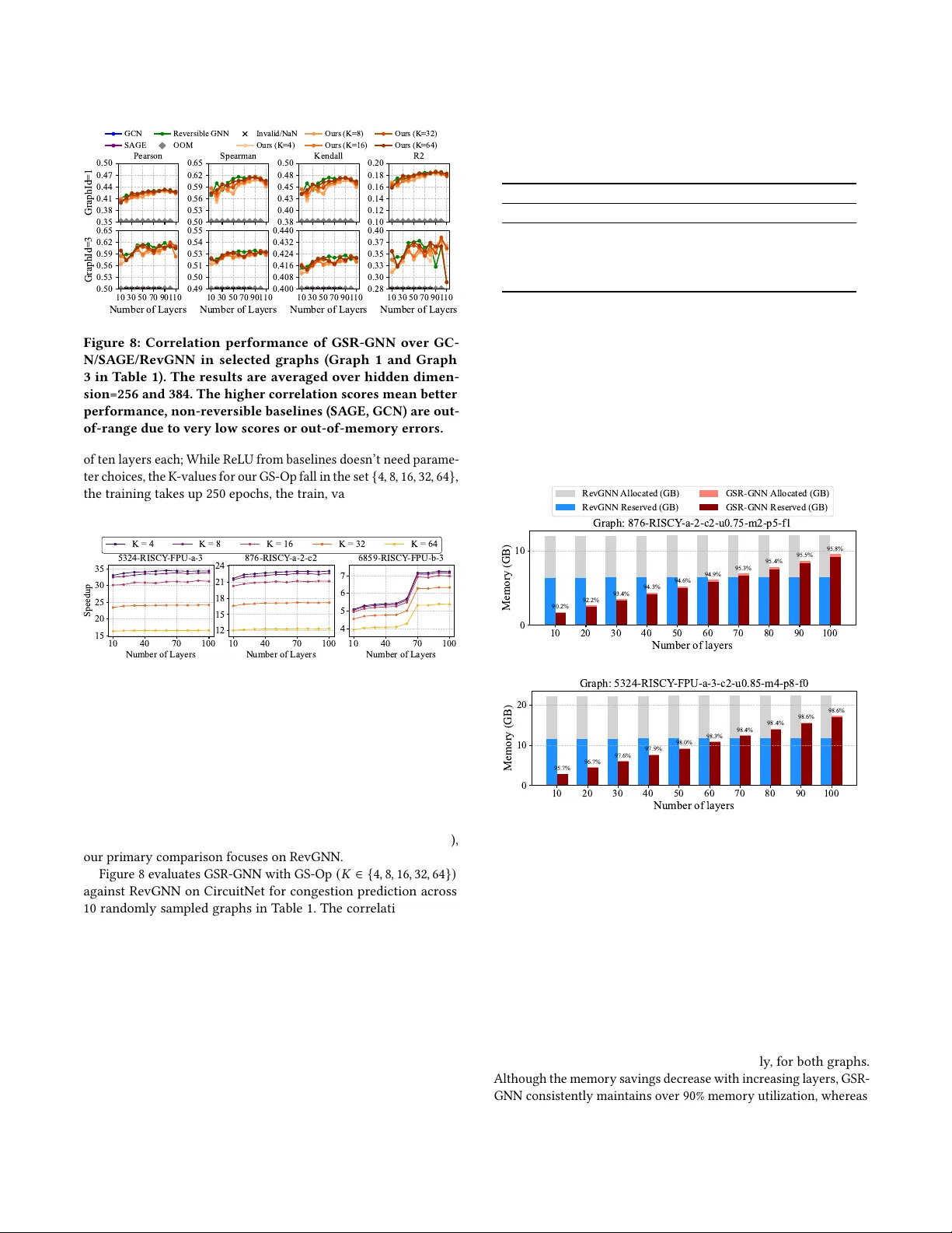
GSR-GNN: T raining Acceleration and Memory-Saving Framework of Deep GNNs on Circuit Graph Y uebo Luo luo00466@umn.edu University of Minnesota, T win Cities Minneapolis, Minnesota, USA Shiyang Li li004074@umn.edu University of Minnesota, T win Cities Minneapolis, Minnesota, USA Yifei Feng yf3005@nyu.edu New Y ork University Brooklyn, New Y ork, USA Vishal Kancharla kanch042@umn.edu University of Minnesota, T win Cities Minneapolis, Minnesota, USA Shaoyi Huang shuang59@stevens.edu Stevens Institute of T echnology Hoboken, New Jersy, USA Caiwen Ding dingc@umn.edu University of Minnesota, T win Cities Minneapolis, Minnesota, USA Abstract Graph Neural Networks (GNNs) show strong promise for circuit analysis, but scaling to modern large-scale circuit graphs is limited by GP U memory and training cost, especially for de ep models. W e revisit deep GNNs for circuit graphs and show that, when trainable, they signicantly outperform shallow architectures, motivating an ecient, domain-specic training framework. W e propose Grouped- Sparse-Reversible GNN (GSR-GNN), which enables training GNNs with up to hundreds of layers while reducing b oth compute and memory overhead. GSR-GNN integrates r eversible residual mod- ules with a group-wise sparse nonlinear operator that compresses node embeddings without sacricing task-relevant information, and employs an optimized execution pipeline to eliminate frag- mented activation storage and reduce data movement. On sampled circuit graphs, GSR-GNN achieves up to 87.2% peak memory reduc- tion and over 30 × training speedup with negligible degradation in correlation-based quality metrics, making deep GNNs practical for large-scale ED A workloads. Ke ywords GNN, ED A, Circuit Design, Reversible Computing 1 Introduction Graph Neural Networks (GNNs) have shown strong and consistent performance in circuit graph analysis [ 14 , 26 ]. For example, verify- ing a Booth multiplier can take over 100 hours using the commercial OneSpin equivalence checking tool [ 23 ], while GNNs can nish the same task in less than one minute. With ongoing technological advances, circuit graphs, graph data extracted from circuit designs, are becoming signicantly larger and more complex [ 5 , 6 , 12 , 13 , 24 ] with greatly varied connection pat- terns. This growth has pushed traditional shallow GNNs—typically 3–4 layers—to their performance limits [10, 28]. Prior research has paved the way for training extremely deep GNNs, reaching hundreds or even thousands of layers. RevGNN [ 18 ], for instance, introduces a group-wise re versible residual structure. It signicantly reduces the memory complexity of GNNs from 𝑂 ( 𝐿 𝑁 𝐷 ) (where 𝐿 is depth, 𝑁 is no des, 𝐷 is features) to 𝑂 ( 𝑁 𝐷 ) , eectively making it independent of depth. Our observations in Figure 1 show that training deep RevGNN leads to signicant p erfor- mance impr ovements in downstream circuit design tasks compar ed 0.0 0.2 0.4 0.410 0.41 1 0.428 OOM OOM Graph 1 Pearson 0.0 0.5 0.587 0.604 0.625 OOM OOM Spearman 0.00 0.25 0.50 0.449 0.462 0.478 OOM OOM Kendall 0.5 0.0 0.166 0.167 0.181 OOM OOM R² 2 3 80 Number of Layers 0.0 0.5 0.609 0.625 0.641 OOM Graph 3 2 3 80 Number of Layers 0.0 0.5 0.543 0.549 0.551 OOM 2 3 80 Number of Layers 0.00 0.25 0.50 0.433 0.437 0.440 OOM 2 3 80 Number of Layers 10 5 0 0.359 0.380 0.407 OOM RevGNN SAGE GCN RevGNN SAGE GCN Figure 1: Performance Comparison: RevGNN vs. SA GE vs. GCN on Circuit Graphs 1 and 3 (Se e T able 1), where RevGNN outperforms SAGE and GCN and keeps gaining return when increasing depth. Negative scores in Spearman, Kendall, and 𝑅 2 mean failure to nd correlations. 10 30 50 70 90 1 10 Number of Layers 0.585 0.590 0.595 0.600 Pearson vs. Layers 10 30 50 70 90 1 10 Number of Layers 0.636 0.638 0.640 0.642 Spearman vs. Layers 10 30 50 70 90 1 10 Number of Layers 0.470 0.472 0.474 0.476 Kendall vs. Layers 10 30 50 70 90 1 10 Number of Layers 0.340 0.350 R-squared vs. Layers Figure 2: Training results of baseline RevGNN on example graph 356-R in T able 1, where RevGNN pleateaus around 70 layers, where SAGE and GCN are either too low to stay in the range or crashed be cause of out-of-memor y (OOM) error . to conventionally shallow GNN architectures, where RevGNN’s Pearson can be pushed to 0.4277 at 80 layers from 0.4096 at two layers, whereas GCN [ 15 ] and GraphSA GE [ 11 ] stay below 0.3731 at best or even zero scores when ther e are two layers. Nonetheless, when approaching its theoretical p otential in circuit design domains, de ep RevGNN hits a scalability bottleneck rooted in its chunk-based, create-then-destroy memor y management strategy . Our proling of RevGNN on the CircuitNet dataset [ 13 ] rev eals that this memory management approach creates a cascade of practical limitations: (i) excessive GP U memor y reservations (e.g., 17910 MB reserved with only 9555.26 MB active, as shown in Figure 3), Y uebo Luo, Shiyang Li, Yifei Feng, Vishal Kancharla, Shaoyi Huang, and Caiwen Ding Active Memory 53.4% 9555.26 MB Non-active Memory Pool 46.6% 8354.74 MB Max Memory Reserved: 17910.00 MB GPU Memory Usage Breakdown Forward 20.8% 5.84 s cudaMemcpy 7.6% 2.13 s Backward 71.6% 20.09 s T otal Runtime per Step: 28.060 s T ime Distribution Each Step Figure 3: GP U memor y usage and epoch runtime summar y of 100-layer RevGNN with 384 hidden channels on Graph 356-RISCY -a1-c5 in Table 1. 10 20 30 40 50 60 70 80 90 100 1 10 Number of Layers 0 2 4 T otal T raining T ime (hours) 0.46 0.91 1.37 1.37 2.28 2.73 3.20 3.65 3.65 3.65 5.10 0.24 0.51 0.78 1.04 1.31 1.57 1.84 2.12 T otal T raining T ime vs. Number of Layers (250 Epochs) RevGNN SAGE GCN OOM Figure 4: Example training time of baseline 100-layer RevGNN on graph 7 in Table 1. Note that the red ’X’ refers to an out-of-memory (OOM) error . prohibitively long training times (5.10 hours for 250 epo chs on a single circuit graph 356-R selected from T able 1, shown in Figure 4), and eventual p erformance degradation in all four correlation scores: Pearson, Spearman, Kendall, and 𝑅 2 beyond optimal depth at around 70 layers (please see Figure 2). Collectively , these issues make Re vGNN practically dicult for real-world circuit congestion prediction tasks. It requires up to 46.4 GP U hours and up to 30+ GB of GP U memory to train a 100-layer , 384-hidden-channel model on just 10 sample d graphs, while the entire dataset has 10,370 dierent circuit graphs in total. T o o vercome these challenges, we streamline RevGNN’s memory management approach, introduce ecient embedding compression with the relative sparse message passing carried by its GNN blocks, and eventually , propose our contributions to the solution as follows: • T o b oost training eciency , we introduce Groupe d-Sparse- Reversible GNN (GSR-GNN), a high-spee d and memory- ecient domain-specic deep GNN framework. GSR-GNN leverages a reversible residual structure to enable deep GNN training. W e further accelerate training by incorporating embedding compression during both for ward and backward passes, without negatively impacting model accuracy . • By optimizing the memory management workow for deep GNN training, we ’ve achieved substantial improvements in memory eciency , maintaining over 90% memory uti- lization and occupying much lower overall memory usage. Our framework also strikes an e xcellent balance between memory usage and training spe ed. Network V isualization 0 250 500 750 Degree 1 0 1 1 0 3 1 0 5 Count Max: 916 Mean: 6.0 Std: 10.4 Degree Distribution 0 2000 4000 6000 8000 Degree 1 0 1 1 0 3 Count Max: 8537 Mean: 238.3 Std: 528.0 Scale-Free (Barabási-Albert, N=60,000) Circuit Graph (356-RISCY -a-1-c) Figure 5: Comparison of Conventional graph dataset (upper) and circuit graph 4 (lower), T able 1 in 50-node graph compo- nent pattern and no de degree distribution. The circuit graph shows an apparently dierent connecting pattern and no de degree distribution from the conventional graph. • W e prole our framework against the domain-specic cir- cuit graph dataset CircuitNet. The evaluation results high- light our framework’s breakneck training spe ed and memor y- saving capabilities in deep GNN training for circuit graph datasets compared to baselines. Experiment results demonstrate that GSR-GNN achie ves up to above 35 × speedup, GP U memory saving of 87 . 22% , and 98 . 6% of reserved memory is active over RevGNN on sampled circuit graph datasets when performing congestion prediction tasks [ 2 , 16 , 27 , 29 ]. 2 Background Graph Learning in Circuit Design: Circuit design workows generate complex circuit representations ideal for graph-base d learning [ 20 , 22 ]. In contrast to a universal graph dataset such as the Barabási– Albert [ 3 ], shown in Figure 5, circuit graphs exhibit unique characteristics: massive nodes, more bi-extreme towards either a few (as few as one) or many neighbours (more than 8,000) per node. Almost even and regular connectivity patterns in the microscope, along with diverse featur e distributions, challenge con- ventional GNN implementations in this domain. Recent eorts have produced comprehensive circuit datasets [ 5 , 13 ] containing thousands of designs for tasks such as congestion prediction [ 8 , 16 ], Design Rules Che ck (DRC), timing estimation, and placement optimization, enabling the realistic evaluation of GNN eciency improvements in terms of computation speedup and end-to-end performance. Reversible GNNs: On top of the residual connection architecture to further the depth of GCN [ 7 , 17 , 19 ], RevGNN [ 18 ] addresses a fundamental memor y bottleneck in training deep GNNs. Traditional deep GNNs suer from pr ohibitive memory overhead that scales linearly with the number of layers, as intermediate activations must be stored for backpropagation. This limits the practical depth of GNNs. RevGNN introduces a reversible architecture [ 9 , 18 ], where the input to each layer can be reconstructed from its output during the backward pass. By eliminating the need to store intermediate activations, RevGNN makes memory complexity independent of network depth, signicantly reducing the memor y overhead during GSR-GNN: Training Acceleration and Memory-Saving Framework of Deep GNNs on Circuit Graph training. This breakthrough enables training GNNs with hundreds of layers on a single GP U . 3 Problem Statement and Challenges In this section, we rst intr oduce the necessar y terminology and notations used in the paper . Then, w e pr esent our obser vations that challenge current RevGNNs. Given graph 𝐺 = ( 𝑉 , 𝐸 ) with adja- cency matrix 𝐴 ∈ R 𝑁 × 𝑁 , node embeddings at layer 𝑙 are denoted as 𝑋 𝑙 ∈ R 𝑁 × 𝐷 , where 𝑁 = | 𝑉 | and 𝐷 is the feature dimension. Net- work depth is 𝐿 with layer index 𝑙 ∈ { 1 , 2 , . . . , 𝐿 } , producing nal predictions ˆ 𝑦 = 𝑓 𝜃 ( 𝑋 𝐿 ) ∈ R 𝑁 . During backpropagation, gradients ow as 𝜕 L 𝜕 ˆ 𝑦 → 𝜕 L 𝜕𝑋 𝐿 → · · · → 𝜕 L 𝜕𝑋 𝑙 . The Split operation partitions tensors along the feature dimension, follow ed by Conventional GNN operations that process full-dimensional node embeddings and gradients: 𝑋 𝑙 1 , 𝑋 𝑙 2 = Split ( 𝑋 𝑙 ) where 𝑋 𝑙 1 , 𝑋 𝑙 2 ∈ R 𝑁 × 𝐷 / 2 (1) 𝑋 𝑙 + 1 = GNN-Block-Forward ( 𝐺 , 𝑋 𝑙 ) (2) 𝜕 L 𝜕𝑋 𝑙 = GNN-Block-Backward ( 𝐺 𝑇 , 𝜕 L 𝜕𝑋 𝑙 + 1 ) (3) where forward pass aggregates neighbor information over 𝐺 , and backward pass propagates gradients through 𝐺 𝑇 . 3.1 Challenges for Reversible GNNs Despite the oretical advantages, reversible GNN faces signicant practical limitations that hinder its adoption in real-world applica- tions. W e identify three critical challenges that motivate the need for more ecient alternatives. Prohibitive Time-for-Space Tradeo: Rev GNN adopts dynamic memory management by partitioning input features X ∈ R 𝑁 × 𝐷 into 𝐶 groups, where 𝑁 = | V | is the number of vertices and 𝐷 is the hidden dimension. This approach employs a create-then- destroy cycle, in terms of detach, copy , and then delete at each layer 𝑡 ∈ [ 1 , 𝐿 ] that incurs signicant overhead. During for ward propagation, activations are immediately deallocated after use: M ( 𝑡 ) input ← ∅ (deallocate via storage.resize(0)) , Peak ( M ) = O  𝑁 · 𝐷 𝐶  (4) During backward propagation, the destroyed inputs must b e re- constructed via memory reallocation and invertible computation: M ( 𝑡 ) input ← resize Ö 𝑖 𝑑 𝑖 ! = malloc ( 𝑁 · 𝐷 · sizeof(oat32) ) , X ( 𝑡 ) input ← 𝑓 − 1 ( Y ( 𝑡 ) ) (5) The frequent allocation-deallocation cycle introduces thr ee sources of overhead: (1) system calls for memory management, (2) mem- ory fragmentation reducing cache eciency , and (3) the invertible computation itself. The grouped reversible architecture computes: Forward: Y ′ 0 = 𝐶  𝑗 = 2 X 𝑗 , Y ′ 𝑖 = 𝑓 𝜃 𝑖 ( Y ′ 𝑖 − 1 , A ) + X 𝑖 , 𝑖 ∈ { 1 , . . . , 𝐶 } (6) Inverse: X 𝑖 = Y ′ 𝑖 − 𝑓 𝜃 𝑖 ( Y ′ 𝑖 − 1 , A ) , Y ′ 𝑖 − 1 =  Y ′ 𝑖 − 1 𝑖 > 1 Í 𝐶 𝑗 = 1 X 𝑗 𝑖 = 1 (7) where each partition X 𝑖 ∈ R 𝑁 × 𝐷 / 𝐶 and 𝑓 𝜃 𝑖 is a GNN block. The inversion requires reverse iteration through all 𝐶 groups. Aggre- gating over 𝐿 layers, without considering the edge embe dding, the total computational complexity is: C total = O  𝐿 ·  𝑁 · 𝐷 2 𝐶   + Θ ( 𝐿 ) (8) where Θ ( 𝐿 ) represents the cumulative allocation overhead. The timing analysis reveals a sever e imbalance, with the total ep och time decomposed as: 𝑇 epoch = 𝑇 forward + 𝑇 copy + 𝑇 backward (9) Empirical Analysis: On a representative EDA b enchmark, for- ward propagation requires 𝑇 forward = 5 . 84 𝑠 ( 20 . 9% ), memory copy (cudaMemcpy ) takes 𝑇 copy = 2 . 13 𝑠 ( 7 . 6% ), while invertible backpr op- agation with repeated reallocation dominates at 𝑇 backward = 20 . 02 𝑠 ( 71 . 6% ), yielding 𝑇 epoch = 27 . 99 𝑠 . The backward-to-forward ratio is 3 . 43 , and the numerical dierence between 𝑇 forward and 𝑇 backward is Δ 𝑇 ≈ 14 . 18 𝑠 per epoch. The backward-to-copy ratio of 9 . 40 further highlights the computational burden from the create-destroy mech- anism. This disproportionate cost can increase total training time by 10 1 to 10 2 × for de ep GNN models ( 𝐿 > 50 ), making RevGNN impractical for time-sensitive EDA applications (e.g., congestion prediction) where rapid design iteration is critical. Diminishing Gain from Extreme Depth: The p erformance ben- ets of very deep Re vGNNs plateau rapidly , particularly on domain- specic graphs. Figure 2 shows that correlation metrics on circuit graphs plateau around 70 layers and deteriorate beyond 100 layers. This indicates that moderate network depth achieves near-optimal performance, questioning the practical value of extreme depth ca- pabilities while compounding the memor y and computational e- ciency challenges described above. 4 Architecture of GSR-GNN In this section, we present our general model ar chitecture design, including our custom operators utilized in GSR-GNN, optimized memory management workow , and our algorithm design in the forward and backward phases. 4.1 Operators and Blocks used in GSR-GNN Suppose the example graph adjacency matrix is  1 0 1 0 0 1 0 1 1 0 0 1 0 1 1 0  , the con- ventional GNN Block of forward and backward pass [ 4 ] performs product full-dimensional no de embedding or gradient processe d by Rectied Linear Units (ReLU [ 1 ]) 𝑅𝑒 𝐿𝑈 ( 𝑋 𝑙 ) in  0 . 37 0 . 76 0 0 . 79 0 . 58 0 0 . 57 0 0 0 . 55 0 . 95 0 0 0 0 . 23 0  and 𝑅𝑒 𝐿𝑈 ( 𝑑 𝑋 𝑙 + 1 𝑑 𝐿 ) in  0 . 23 0 0 . 89 0 0 . 45 0 . 78 0 0 . 67 0 0 0 0 . 88 0 0 . 33 0 . 66 0  , resulting in  0 . 37 1 . 31 0 . 95 0 . 79 0 . 58 0 0 . 8 0 0 . 37 0 . 76 0 . 23 0 . 79 0 . 58 0 . 55 1 . 52 0  and  0 . 23 0 0 . 89 0 . 38 0 . 56 1 . 11 0 . 66 0 . 67 0 . 23 0 . 33 1 . 55 0 0 . 45 1 . 11 0 1 . 05  as 𝑋 𝑙 + 1 and 𝑑 𝑋 𝑙 𝑑 𝐿 respectively . In contrast, our GSR- GNN Block introduces Group Sparse GS ( 𝑋 , 𝑘 ) → ( 𝑉 , 𝐼 ) as a coun- terpart to ReLU. Where values 𝑉 ∈ R 𝑁 × 𝑘 and indices 𝐼 ∈ Z 𝑁 × 𝑘 are equivalent to sparsifying the node embedding with pre-dened 𝑘 values, which is V al:  0 . 79 0 . 58 0 . 95 0 . 86  and Idx:  3 0 2 3  for forward block example, where each row of val is the K-most signicant elements selected from full-dimentional node embedding. And V al :  0 . 12 0 . 45 0 . 55 0 . 99  for the back- ward blo ck example while keeping the same val saved since forward. The indices 𝐼 / idx record the "activated" neurons’ p ositions to source 𝑉 / val in the embedding from the forward pass. It is preserved and used in the backward process to source the gradient that shares the same positions as in the embedding; this step is an indispens- able contributing factor to performance. Then, our sparse message Y uebo Luo, Shiyang Li, Yifei Feng, Vishal Kancharla, Shaoyi Huang, and Caiwen Ding 0.17 0.40 0.07 0.49 0.45 0.21 0.73 0.15 3.8 0 3.38 0 Group 2 Group 1 1.55 0.58 1.86 0.14 0.76 0.31 0.55 0.02 0.37 0.58 0.92 0.14 1 0 0 1 1 0 0 1 1 0 0 1 0 1 1 0 0 0 0 1 1 0 0 1 1 0 0 1 0 1 1 0 0 0 0 1 1 0 0 1 1 0 0 1 0 1 1 0 1 1 0 0 0 1 1 0 0 1 1 0 0 1 0 1 1 0 1 0.45 0.40 0.73 0.49 1.18 0.89 0.94 1.13 0.45 0.40 0.73 0.49 0 1 0 1 0 0 0 0 0.40 0.49 0.45 0.73 0 0 0 0 Idx 0.58 0.14 0.76 0.55 1.55 1.86 1.2 1.15 0.76 0.31 0.55 0.02 0.37 0.58 0.92 0.14 1.55 1.2 1.86 1.15 3.35 2.35 2.65 3.06 0 0 0 0 1.55 1.86 1.15 0 1 0 1 1.2 0 2.75 0 3.55 3.8 0 3.38 0 0 2.75 0 3.55 0.76 1.2 0.55 1.15 GSR-GNN Grouped Conv Foward GSR-GNN Forward Not Saved For Backward Propagation V al Idx V al Idx Idx 0 1 0 1 Idx 0 1 0 1 Idx V al V al GS-Op GS-Op Step 1: Group Partition Step 2: Grouped Forward Step 3: Groups Stacked GSR-GNN Forward Group 1 GSR-Forward Group 2 GSR-Forward 1 1 2 3 4 6 8 5 7 8 Group 2 Group 1 1.18 0.94 0.89 1.13 3.35 2.65 2.35 3.06 Figure 6: GSR-GNN in-layer for ward workow . 0 0 -0.61 -1.1 1 1.89 0 0.66 0 -0.74 -0.98 0 0 0 1.95 0 3.18 0 0 0 1 1 0 0 1 1 0 0 1 0 1 1 0 1 0 0 0 1 1 0 0 1 1 0 0 1 0 1 1 0 1 0.37 1.66 1.52 0.29 1.89 1.95 0.66 3.18 0 0 0 0 0 1 0 1 1 1 0 0 Idx V al Idx Saved For Step 3 -0.53 0.07 -0.76 0.83 0.15 -0.94 0.45 -0.08 Group 1 Group 2 -0.82 0.68 -0.13 0.29 0.37 -0.21 0.91 -0.62 1 0 0 1 1 0 0 1 1 0 0 1 0 1 1 0 0 0 0 1 1 0 0 1 1 0 0 1 0 1 1 0 0 0 0 1 1 0 0 1 1 0 0 1 0 1 1 0 1 1 0 0 0 1 1 0 0 1 1 0 0 1 0 1 1 0 1 0.37 0.68 0.91 0.29 1.28 0.97 0.66 1.59 0.37 0.68 0.91 0.29 0 1 0 1 Equivalent T o 0 0 0 0 Idx -0.53 0.07 -0.76 0.83 0.15 -0.94 0.45 -0.08 -0.53 -0.9 -0.21 -0.08 0 0 0 0 1 1 0 0 0.74 1.66 0 0.29 0.37 0 1.52 1.11 GSR-GNN Forward V al Idx V al Idx Idx 1 1 0 0 Idx 0 1 0 1 Idx V al V al GSR-GNN Grouped Conv Backward GS-Op GS-Op GSR-GNN Forward 1 1 0 0 Idx Step 1: Group Partition Step 4: Groups Stacked Idx GS-Op: Grouped Sparse Opearator 0 1 0 2 3 3 2 3 V al Idx -1.13 -0.94 -0.21 -0.08 -0.53 -0.9 -0.76 -0.76 Group 2 GSR-Forward Group 1 GSR-Forward Group 2 GSR-Backward Group 1 GSR-Backward Idx 0 1 0 1 0.74 0 0 1.11 1.66 0.29 0.37 1.52 Idx 0 1 0 1 -0.53 -0.21 -0.08 -0.9 - -0.74 -0.98 -0.61 -1.11 -0.53 -0.9 -0.21 -0.08 -0.74 -0.98 -0.61 -1.11 Step 3: Grouped Sparse Backward 0 0 0 0 Step 2: Grouped Inverted Backward Saved For Step 3 Saved Since Step 2 GSR-GNN Backward 0 0 0 0 -1.13 -0.94 -0.76 -0.76 -0.21 -0.08 -0.53 -0.9 1 1 2 3 3 4 5 6 1 2 3 3 V al Idx 0 0 -0.21 -0.08 -0.53 -0.9 0 0 Group 1 Group 2 -0.61 -1.11 -0.74 -0.98 -0.61 -1.11 -0.74 -0.98 1.28 0.66 0.97 1.59 0.68 0.29 0.37 0.91 1.89 0.66 1.95 3.18 Figure 7: GSR-GNN in-layer backward workow . passing occurs via: 𝑋 𝑙 + 1 = GSR-GNN-For war d-Block ( 𝑉 𝑙 , 𝐼 𝑙 , 𝐺 ) (10) 𝜕 L 𝜕𝑋 𝑙 = GSR-GNN-Backward-Block ( 𝑀 𝑙 , 𝐼 𝑙 , 𝐺 ) (11) Then, 𝑋 𝑙 + 1 is  0 0 0 . 95 0 . 79 0 . 58 0 0 0 . 86 0 0 0 1 . 65 0 . 58 0 0 . 95 0  and 𝜕 L 𝜕𝑋 𝑙 becomes  0 0 0 . 67 0 1 . 44 0 0 0 0 0 1 . 11 0 0 0 0 1 . 0  through product and scatter . With ( 𝑉 , 𝐼 ) , our for ward block promptly uses values in the node embedding indexed by the indices while skipping zero elements, rather than accessing full-dimensional embe ddings per node when it comes to the partially reversible backward phase. Similarly , the GSR-GNN backward block also eciently utilizes 𝐼 generated in the forward block to record neurons’ positions for reference, so the corresponding backward block only reads the gradients whose positions are recorded by 𝐼 to compute and then nish one learning step. Algorithm 1 GSR-GNN Forward 1: Input: Graph 𝐺 , features 𝑋 0 , layers 𝐿 , GS parameter 𝑘 2: Output: Predictions ˆ 𝑦 3: for 𝑙 = 1 to 𝐿 do 4: 𝑋 𝑙 1 , 𝑋 𝑙 2 ← Split ( 𝑋 𝑙 − 1 ) ; 5: 𝑉 𝑙 1 , 𝐼 𝑙 1 ← GS ( 𝑋 𝑙 1 , 𝑘 ) ⊲ Group partition & GS 6: 𝑀 𝑙 1 ← GSR - For ward ( 𝑉 𝑙 1 , 𝐼 𝑙 1 , 𝐺 ) 7: 𝑋 𝑙 + 1 2 ← 𝑋 𝑙 2 + 𝑀 𝑙 1 8: 𝑉 𝑙 2 , 𝐼 𝑙 2 ← GS ( 𝑋 𝑙 + 1 2 , 𝑘 ) 9: 𝑀 𝑙 2 ← GSR - For ward ( 𝑉 𝑙 2 , 𝐼 𝑙 2 , 𝐺 ) 10: 𝑋 𝑙 + 1 1 ← scaer ( 𝑉 𝑙 1 , 𝐼 𝑙 1 ) + 𝑀 𝑙 2 11: 𝑋 𝑙 + 1 ← Concat ( 𝑋 𝑙 + 1 1 , 𝑋 𝑙 + 1 2 ) ⊲ Stack groups 12: end for 13: return OutputLayer ( 𝑋 𝐿 ) 4.2 Enhanced Memory Management Our GSR-GNN framework changes the in-group worko w com- pared to conventional RevGNN. Unlike RevGNN’s frequent detach- copy-delete cycles for both node embeddings (forward pass) and gradient tensors ( backwar d pass), our custom blocks eliminate these costly memory operations. GSR-GNN: Training Acceleration and Memory-Saving Framework of Deep GNNs on Circuit Graph Algorithm 2 GSR-GNN Backward 1: Input: Gradient 𝜕 𝐿 / 𝜕 ˆ 𝑦 Output: Gradient 𝜕 𝐿 / 𝜕𝑋 0 2: 𝑔 𝐿 ← OutputLayerBackward ( 𝜕𝐿 / 𝜕 ˆ 𝑦 ) 3: for 𝑙 = 𝐿 down to 1 do 4: ( 𝑔 𝑙 + 1 1 , 𝑔 𝑙 + 1 2 ) ← Split ( 𝑔 𝑙 + 1 ) ; ( 𝑉 2 , 𝐼 2 ) ← GS ( 𝑔 𝑙 + 1 2 , 𝑘 ) ⊲ Group partition & GS 5: 𝑀 1 ← 𝑔 𝑙 + 1 1 − GSRBlock ( 𝑉 2 , 𝐼 2 , 𝐺 ) 6: ( 𝑉 1 , 𝐼 1 ) ← GS ( 𝑀 1 , 𝑘 ) ; 𝑍 1 ← GSRBlock ( 𝑉 1 , 𝐼 1 , 𝐺 ) 7: 𝑀 2 ← 𝑉 2 . scatter ( 𝐼 2 ) − 𝑍 1 8: 𝑔 𝑙 1 ← GSRBlockBackward ( 𝑀 1 , 𝐼 1 , 𝐺 ) ; 𝑔 𝑙 2 ← GSRBlockBackward ( 𝑀 2 , 𝐼 2 , 𝐺 ) 9: 𝑔 𝑙 ← Concat ( 𝑔 𝑙 1 , 𝑔 𝑙 2 ) 10: end for 11: Return 𝑔 0 This optimization yields three key b enets: (1) reduced frag- mentation by avoiding unnecessary tensor copies, (2) improved memory utilization through elimination of inactive memor y pools, and (3) selective save-for-backward op erations that only store indices when required for subsequent backward blocks. While our appr oach maintains 𝑂 ( 𝐿𝑁 𝐾 ) memory complexity lin- ear in the number of layers 𝐿 , the actual memory footprint remains signicantly lower than RevGNN within the practical depth range. This design ensures predictable memory usage while maximizing GP U memory eciency for deep graph neural networks. 4.3 Forward Phase of GSR-GNN Figure 6 and 7 provide an overview of GSR-GNN. For each layer , dur- ing the forward propagation shown in Figure 6, the input node em- bedding is partitioned evenly into two groups, split  0 . 37 0 . 76 0 . 45 0 . 17 0 . 58 0 . 31 0 . 21 0 . 40 0 . 92 0 . 55 0 . 73 0 . 07 0 . 14 0 . 02 0 . 15 0 . 49  =  0 . 37 0 . 76 0 . 58 0 . 31 0 . 92 0 . 55 0 . 14 0 . 02   0 . 45 0 . 17 0 . 21 0 . 40 0 . 73 0 . 07 0 . 15 0 . 49  . This is step 1 ○ from line 5, Algorithm 1. Group 1  0 . 45 0 . 17 0 . 21 0 . 40 0 . 73 0 . 07 0 . 15 0 . 49  rstly proceeds through the GS-Op at 2 ○ (line 5, Algo- rithm1) to produce the compressed CBSR-format V al:  0 . 45 0 . 40 0 . 73 0 . 49  , idx:  0 1 0 1  , which become the input of the GSR-GNN forward block rst ( 3 ○ , line 6 of Algorithm 1), then the result  1 . 18 0 0 0 . 89 0 . 94 0 0 1 . 13  added to Group 2  0 . 45 0 . 17 0 . 21 0 . 40 0 . 73 0 . 07 0 . 15 0 . 49  , which subsequently enters the second GS-Op at 5 ○ at line 8 and produces V al:  1 . 55 1 . 2 1 . 86 1 . 15  and Idx:  0 1 0 1  , then another forward block at 6 ○ , line 9. Following this, the output of the second forward block  3 . 35 0 0 2 . 35 2 . 65 0 0 3 . 06  is also added back to group 1 at 7 ○ to be the up dated channel 1, shown by line 10, 11 of Algorithm1, meanwhile becomes the update d channel 2 of the node embe dding at 8 ○ with the up- dated group 1, 𝑋 𝑙 + 1 1 =  3 . 8 0 0 2 . 75 3 . 38 0 0 3 . 55  , this also updates channel 2 of the node embedding to b e passed to the next layer . 4.4 Backward P hase of GSR-GNN During the backward propagation in Figure 7 and Algorithm 2, the gradient passed from the next layer is split into two groups split  0 . 37 − 0 . 82 0 . 15 − 0 . 53 − 0 . 21 0 . 68 − 0 . 94 0 . 07 0 . 91 − 0 . 13 0 . 45 − 0 . 76 − 0 . 62 0 . 29 − 0 . 08 0 . 83  =  0 . 37 − 0 . 82 − 0 . 21 0 . 68 0 . 91 0 . 13 − 0 . 62 0 . 29  ,  0 . 15 − 0 . 53 − 0 . 94 0 . 07 0 . 45 − 0 . 76 − 0 . 08 0 . 83  (step 1 ○ , line 4, Al- gorithm2), whereas, at this time, group 2  0 . 37 − 0 . 82 − 0 . 21 0 . 68 0 . 91 0 . 13 − 0 . 62 0 . 29  goes through T able 1: Circuit Graph Dataset Summar y (Ordered by Size) Size # Name Node Edge Train/V al/Test Lab els Range L 1 5324-F 69.8k 22.5M 48.8/10.5/10.5k 131 [0.0, 1.0] 2 4474-F 65.3k 21.8M 52.3/6.5/6.5k 255 [0.0, 1.04] M 3 876-R 49.6k 12.2M 39.7/5.0/5.0k 60 [0.0, 0.22] 4 1522-R 49.5k 12.2M 39.6/5.0/5.0k 106 [0.0, 0.36] 5 1886-R 49.1k 11.7M 39.3/4.9/4.9k 134 [0.0, 0.58] 6 639-R 49.1k 11.7M 34.3/7.4/7.4k 105 [0.0, 0.48] 7 356-R 49.0k 11.7M 39.2/4.9/4.9k 271 [0.0, 0.90] S 8 6859-F 44.3k 2.7M 35.4/4.4/4.4k 28 [0.0, 1.0] 9 6227-F 43.4k 2.7M 34.7/4.3/4.3k 148 [0.0, 3.75] 10 7157-R 38.7k 6.8M 30.9/3.9/3.9k 153 [0.0, 0.66] Note: "F" and "R" in the column Name refer to "FP U" and "RISC- Y" . GS-Op to output CBSR values  0 . 37 0 . 68 0 . 91 0 . 29  and indices  0 1 0 1  at 2 ○ , and enter the GSR-GNN forward block at 3 ○ at line 5 in Algorithm 2 and note that positions (indices) of the activated neurons are saved for the step at line 8. Then, the output of the rst for ward block  1 . 28 0 0 0 . 97 0 . 66 0 0 1 . 59  goes to the subtraction with group 1 ( line 7, Alg 2), the result  1 . 13 0 . 53 0 . 94 0 . 9 0 . 21 0 . 76 0 . 08 0 . 76  goes into two ways: one enters another GS-Op at 4 ○ with the result  − 0 . 53 − 0 . 9 − 0 . 21 − 0 . 08  and indices  1 1 0 0  , which enter the second forward block at 5 ○ , whose result  0 − 0 . 74 0 − 0 . 98 − 0 . 61 0 − 1 . 11 0  performs subtraction with group 2 at 6 ○ to be the input of its GSR-GNN backward block at 1 ; the other is kept for the dedicated backward blo ck at 2 . This process is covered by lines 8 in Algorithm 2. Using the remem- bered positions from the previous forward-style recomputation, both channels of the gradient 𝜕𝐿 𝜕𝑋 𝑙 1  1 . 89 0 0 1 . 95 0 . 66 0 0 3 . 18  and 𝜕𝐿 𝜕𝑋 𝑙 2  0 − 0 . 74 0 − 0 . 98 − 0 . 61 0 − 1 . 11 0  are updated to be passe d to the last lay er at 3 . 5 Experiments This section presents our experimental setup and evaluates the per- formance of GSR-GNN against baseline methods. W e demonstrate the framework’s advantages in terms of training acceleration and memory eciency while maintaining comparable accuracy . Platform: All experiments were conducted on an AMD EPY C 7763 64-Core Processor ser ver (504GB RAM) and a single N VIDIA A6000- 48GB GP U (CUD A toolkit 12.6), PyG version 2.5.0, Pytorch 2.1.2. Dataset: W e evaluate our approach using the CircuitNet dataset [ 5 ], which originates from over 10,000 circuit graph samples ser ving various downstream tasks. W e randomly sample 10 representative circuit designs (detailed in T able 1) following the provided pre- processing metho d without sub-graph partitioning to ensure design size variability and fully expose the scale of graph data. W e focus primarily on congestion prediction, a critical step in the circuit design process [ 5 , 13 , 22 ]. Following standard practice in circuit design applications [ 25 ], we evaluate performance using thr ee rank correlation metrics: Pearson, Kendall, and Spearman correlation scores, with higher values indicating better performance. Models and Conguration: W e compared our mo del with state- of-the-art GraphSAGE [ 21 ], GCN [ 15 ], and the ocial RevGNN [ 18 ]. The hyperparameters include: hidden dimension, var ying between 256 and 384; the number of layers, ranging from 10 to 100 with a step Y uebo Luo, Shiyang Li, Yifei Feng, Vishal Kancharla, Shaoyi Huang, and Caiwen Ding 0.35 0.38 0.41 0.44 0.47 0.50 GraphId=1 Pearson 0.50 0.53 0.56 0.59 0.62 0.65 Spearman 0.38 0.40 0.43 0.45 0.48 0.50 Kendall 0.10 0.12 0.14 0.16 0.18 0.20 R2 10 30 50 70 90 1 10 Number of Layers 0.50 0.53 0.56 0.59 0.62 0.65 GraphId=3 10 30 50 70 90 1 10 Number of Layers 0.49 0.50 0.51 0.53 0.54 0.55 10 30 50 70 90 1 10 Number of Layers 0.400 0.408 0.416 0.424 0.432 0.440 10 30 50 70 90 1 10 Number of Layers 0.28 0.30 0.33 0.35 0.37 0.40 GCN SAGE Reversible GNN OOM Invalid/NaN Ours (K=4) Ours (K=8) Ours (K=16) Ours (K=32) Ours (K=64) Figure 8: Correlation performance of GSR-GNN over GC- N/SA GE/RevGNN in selected graphs (Graph 1 and Graph 3 in T able 1). The results are averaged over hidden dimen- sion=256 and 384. The higher correlation scores mean better performance, non-reversible baselines (SAGE, GCN) are out- of-range due to very low scores or out-of-memory errors. of ten layers each; While ReLU from baselines doesn’t need parame- ter choices, the K-values for our GS-Op fall in the set { 4 , 8 , 16 , 32 , 64 } , the training takes up 250 epochs, the train, validation and test set division are given in T able 1. 10 40 70 100 Number of Layers 15 20 25 30 35 Speedup 5324-RISCY -FPU-a-3 10 40 70 100 Number of Layers 12 15 18 21 24 876-RISCY -a-2-c2 10 40 70 100 Number of Layers 4 5 6 7 6859-RISCY -FPU-b-3 K = 4 K = 8 K = 16 K = 32 K = 64 Figure 9: Speedup of GSR-GNN over Reversible GNNs at var y- ing sparsity levels dene d by 𝐾 , the greater the 𝐾 , the more elements preser v ed per row of activations and lower sparsity . 5.1 Experimental Results This section demonstrates that GSR-GNN achieves training accel- eration while maintaining comparable correlation performance to standard rev ersible deep GNN models. Given that non-reversible GCN and SAGE mo dels exhibit severe performance uctuations with increasing depth and r emain inferior to RevGNN (Figure 1), our primary comparison focuses on RevGNN. Figure 8 evaluates GSR-GNN with GS-Op ( 𝐾 ∈ { 4 , 8 , 16 , 32 , 64 }) against RevGNN on CircuitNet for congestion prediction across 10 randomly sample d graphs in Table 1. The correlation metrics demonstrate that GSR-GNN maintains performance comparable to RevGNN, with mean dierences of +0.0026 (Pearson), +0.0067 (Spearman), +0.0053 (Kendall), and -0.023 ( 𝑅 2 ). These negligible dierences indicate that GS-Op preserves model accuracy while enabling the observed spe edups. Figure 9 illustrates the end-to-end training speedup of GSR-GNN at two hidden channels, 256 and 384, over RevGNN across three cir- cuit scales. GSR-GNN achieves over 35 × (K=4, 384 hidden channels) for graph 5324-RISCY -FP U-a-3, over 4 × (K=64) for graph 6859- RISCY -FP U-b-3, with performance inversely correlated to sparsity level. In addition, we r evisit the breakdown of training step runtime T able 2: Runtime Distribution: 100-layer , 384-hidden chan- nels Baseline (RevGNN) vs Ours (Graph 3 in T able 1) Method Forward ↓ Backwar d ↓ cudaMemCpy ↓ Total/Spdup ↑ Baseline 5.84s (20.8%) 20.09s (71.6%) 2.13s (7.6%) 28.06s Ours (K=4) 0.36s (23.7%) 1.16s (76.2%) 0.001s (0.1%) 1.52s (18.4 × ) Ours (K=8) 0.37s (24.2%) 1.17s (75.7%) 0.001s (0.1%) 1.54s (18.2 × ) Ours (K=16) 0.40s (24.1%) 1.25s (75.9%) 0.001s (0.1%) 1.64s (17.1 × ) Ours (K=32) 0.50s (24.1%) 1.59s (75.9%) 0.001s (0.1%) 2.09s (13.4 × ) Ours (K=64) 0.76s (24.7%) 2.31s (75.2%) 0.001s (0.1%) 3.07s (9.1 × ) since Figure 3, comparing our GSR-GNN against RevGNN on the same graph dataset 356-RISCY -a1-c5. T able 2 shows that GSR-GNN has obvious acceleration across three sections: Forward, Backward, and cudaMemCpy . The most signicant training component, Backward, is r educed to 1.52 sec- onds at b est, and forward is 0.36 seconds. Our memory management optimization consistently cuts cudaMemcpy time to 0.0001 seconds during the whole training w orkow , making a nal best speedup of 18 . 4 × . Though increasing sparsity in terms of 𝐾 lowers the r elative speedup ee ct, the w orst end-to-end spee dup can still r each 9 . 1 × . 10 20 30 40 50 60 70 80 90 100 Number of layers 0 10 Memory (GB) 90.2% 92.2% 93.4% 94.3% 94.6% 94.9% 95.3% 95.4% 95.5% 95.8% Graph: 876-RISCY -a-2-c2-u0.75-m2-p5-f1 RevGNN Allocated (GB) RevGNN Reserved (GB) GSR-GNN Allocated (GB) GSR-GNN Reserved (GB) (a) 876-RISCY -a-2-c2-u0.75-m2-p5-f1 10 20 30 40 50 60 70 80 90 100 Number of layers 0 10 20 Memory (GB) 95.7% 96.7% 97.6% 97.9% 98.0% 98.3% 98.4% 98.4% 98.6% 98.6% Graph: 5324-RISCY -FPU-a-3-c2-u0.85-m4-p8-f0 RevGNN Allocated (GB) RevGNN Reserved (GB) GSR-GNN Allocated (GB) GSR-GNN Reserved (GB) (b) 5324-RISCY-FPU-a-3-c2-u0.85-m4-p8-f0 Figure 10: Memory eciency comparison b etween RevGNN and GSN-GNN on 2 sample graphs, graph 1 and graph 3 in T able 1. The memor y eciency , expressed as a percentage, is the ratio of Allocated GP U Memor y to Reser v ed GP U Mem- ory during the training phase of mo dels. Furthermore, Figure 10 pr esents the memory eciency of GSR- GNN compared to RevGNN on graph 876-R and 5324-R from T able 1. Due to optimized memor y management and compressed node embeddings, within the optimal range of the number of layers, GSR-GNN consistently consumes less GP U memor y than RevGNN, even at 100 layers. GSR-GNN comes with a clear , minimum gap of on average 2.58GB and 5.043GB, respectively , for both graphs. Although the memor y savings decrease with increasing layers, GSR- GNN consistently maintains ov er 90% memory utilization, whereas GSR-GNN: Training Acceleration and Memory-Saving Framework of Deep GNNs on Circuit Graph RevGNN always exhibits approximately 50% memory waste. This shows that our GSR-GNN reduces the maximum number of GNNs that can be trained on circuit graph datasets of various sizes. A d- ditionally , this enables training of circuit graph datasets on GP Us with less than 8 GB of memory at layers less than 30. T o be closer to baseline performance while maintaining relative speedup, one can also increase b oth layers and lower the sparsity to achieve near-optimal performance in correlation metrics. 6 Conclusion In our paper , we propose a GNN training framework targeting faster and more GP U memory-ecient deep GNN training on cir- cuit graph datasets. W e redesign the grouped convolution and re- versible residual module of RevGNN with custom grouped sparse reversible GNN blocks and applied it to graph datasets sampled from CircuitNet in varied, representative sizes. In the evaluation on target circuit graph datasets, our framework achieves apparent training acceleration eect (over 35 × at most), lower GP U memory reservation ( 87 . 22% GP U memory saving at most), and higher e- ciency (98.6% rate of active memory over total r eversed memory), with almost unchanged performance in correlation metrics from the congestion prediction task. Acknowledgments This research was supported in part by NSF SHF-2505770. References [1] Abien Fred Agarap. 2019. Deep Learning using Rectied Linear Units (ReLU). arXiv:1803.08375 [cs.NE] https://arxiv .org/abs/1803.08375 [2] Mohamed Baker Alawieh, Wuxi Li, Yibo Lin, Love Singhal, Mahesh A Iyer , and David Z Pan. 2020. High-denition routing congestion prediction for large- scale FPGAs. In 2020 25th Asia and South Pacic Design Automation Conference (ASP-D AC) . IEEE, 26–31. [3] Réka Albert and Albert-László Barabási. 2002. Statistical mechanics of complex networks. Reviews of Modern Physics 74, 1 (Jan. 2002), 47–97. doi:10.1103/ revmodphys.74.47 [4] Shaojie Bai, J. Zico Kolter , and Vladlen K oltun. 2019. Deep Equilibrium Mo dels. arXiv:1909.01377 [cs.LG] https://arxiv .org/abs/1909.01377 [5] Zhuomin Chai, Y uxiang Zhao, W ei Liu, Yibo Lin, Runsheng Wang, and Ru Huang. 2023. CircuitNet: An Open-Source Dataset for Machine Learning in VLSI CAD Applications With Improved Domain-Specic Evaluation Metric and Learning Strategies. IEEE Transactions on Computer-Aided Design of Integrated Circuits and Systems 42, 12 (2023), 5034–5047. doi:10.1109/TCAD.2023.3287970 [6] Animesh Basak Chowdhury , Benjamin T an, Ramesh Karri, and Siddharth Garg. 2021. Op enABC-D: A Large-Scale Dataset For Machine Learning Guided Inte- grated Circuit Synthesis. arXiv:2110.11292 [cs.LG] https://ar xiv .org/abs/2110. 11292 [7] Laurent Dinh, David Krueger , and Y oshua Bengio. 2015. NICE: Non-linear Independent Components Estimation. arXiv:1410.8516 [cs.LG] https://arxiv .org/ abs/1410.8516 [8] Amur Ghose, Vincent Zhang, Yingxue Zhang, Dong Li, Wulong Liu, and Mark Coates. 2021. Generalizable cross-graph embedding for GNN-based congestion prediction. In 2021 IEEE/ACM International Conference On Computer Aided Design (ICCAD) . IEEE, 1–9. [9] Aidan N Gomez, Mengye Ren, Raquel Urtasun, and Roger B Grosse . 2017. The reversible residual network: Backpropagation without storing activations. Ad- vances in neural information processing systems 30 (2017). [10] Zizheng Guo, Mingjie Liu, Jiaqi Gu, Shuhan Zhang, David Z. Pan, and Yibo Lin. 2022. A timing engine inspired graph neural network model for pre-routing slack prediction. In Proceedings of the 59th ACM/IEEE Design Automation Conference (San Francisco, California) (DA C ’22) . Association for Computing Machinery , New Y ork, N Y , USA, 1207–1212. doi:10.1145/3489517.3530597 [11] William L. Hamilton, Rex Ying, and Jure Leskovec. 2018. Inductive Representation Learning on Large Graphs. arXiv:1706.02216 [cs.SI] https://arxiv .org/abs/1706. 02216 [12] W eihua Hu, Matthias Fey , Marinka Zitnik, Yuxiao Dong, Hongyu Ren, Bowen Liu, Michele Catasta, and Jure Leskovec. 2020. Open graph benchmark: Datasets for machine learning on graphs. Advances in neural information processing systems 33 (2020), 22118–22133. [13] Xun Jiang, zhuomin chai, Yuxiang Zhao, Yibo Lin, Runsheng Wang, and Ru Huang. 2024. CircuitNet 2.0: An Advanced Dataset for Promoting Machine Learning Innovations in Realistic Chip Design Environment. In The T welfth International Conference on Learning Representations . https://openreview .net/ forum?id=nMFSUjxMIl [14] Daniela Kaufmann. 2022. Formal verication of multiplier circuits using com- puter algebra. it - Information T echnology 64, 6 (2022), 285–291. doi:doi: 10.1515/itit- 2022- 0039 [15] Thomas N. Kipf and Max W elling. 2017. Semi-Super vised Classication with Graph Convolutional Networks. In 5th International Conference on Learning Representations, ICLR 2017, Toulon, France, A pril 24-26, 2017, Conference Track Proceedings . OpenReview .net. https://openreview .net/forum?id=SJU4ayY gl [16] Robert Kirby , Saad Godil, Rajarshi Roy, and Bryan Catanzaro. 2019. Congestion- Net: Routing congestion prediction using deep graph neural networks. In 2019 IFIP/IEEE 27th International Conference on V ery Large Scale Integration (VLSI-SoC) . IEEE, 217–222. [17] Guohao Li, Matthias Muller , Ali Thabet, and Bernard Ghanem. 2019. De epGCNs: Can GCNs go as deep as CNNs?. In Procee dings of the IEEE/CVF international conference on computer vision . 9267–9276. [18] Guohao Li, Matthias Müller, Bernard Ghanem, and Vladlen Koltun. 2022. T raining Graph Neural Networks with 1000 Layers. arXiv:2106.07476 [cs.LG] https: //arxiv .org/abs/2106.07476 [19] Guohao Li, Chenxin Xiong, Ali Thabet, and Bernard Ghanem. 2020. Deepergcn: All you need to train deeper gcns. arXiv preprint arXiv:2006.07739 (2020). [20] Yibo Lin, Zixuan Jiang, Jiaqi Gu, Wuxi Li, Shounak Dhar , Haoxing Ren, Brucek Khailany , and David Z. Pan. 2021. DREAMPlace: Deep Learning T o olkit-Enabled GP U Acceleration for Modern VLSI Placement. IEEE Transactions on Computer- Aided Design of Integrated Circuits and Systems 40, 4 (2021), 748–761. doi:10.1109/ TCAD.2020.3003843 [21] Jielun Liu, Ghim Ping Ong, and Xiqun Chen. 2020. GraphSAGE-based trac speed forecasting for segment network with sparse data. IEEE Transactions on Intelligent Transportation Systems 23, 3 (2020), 1755–1766. [22] Martin Rapp, Hussam Amrouch, Yibo Lin, Bei Yu, David Z. Pan, Marilyn W olf, and Jörg Henkel. 2022. MLCAD: A Sur v ey of Research in Machine Learning for CAD Keynote Paper . IEEE Transactions on Computer-Aided Design of Integrated Circuits and Systems 41, 10 (2022), 3162–3181. doi:10.1109/TCAD.2021.3124762 [23] Amr Sayed- Ahmed, Daniel Große, Ulrich Kühne, Mathias Soeken, and Rolf Drechsler . 2016. Formal verication of integer multipliers by combining Gröbner basis with logic reduction. In 2016 Design, Automation & T est in Europe Conference & Exhibition (DA TE) . 1048–1053. [24] Kuansan W ang, Zhihong Shen, Chiyuan Huang, Chieh-Han Wu, Y uxiao Dong, and Anshul Kanakia. 2020. Microsoft Academic Graph: When ex- perts are not enough. Quantitative Science Studies 1, 1 (02 2020), 396–413. arXiv:https://direct.mit.edu/qss/article-pdf/1/1/396/1760880/qss_a_00021.pdf doi:10.1162/qss_a_00021 [25] Shuwen Y ang, Zhihao Y ang, Dong Li, Yingxue Zhang, Zhanguang Zhang, Guojie Song, and Jianye HA O. 2022. V ersatile Multi-stage Graph Neural Network for Circuit Representation. In Advances in Neural Information Processing Systems , Alice H. Oh, Alekh Agarwal, Danielle Belgrave, and K yunghyun Cho (Eds.). https://openreview .net/forum?id=nax3A TLrovW [26] Cunxi Yu, Maciej Ciesielski, and Alan Mishchenko. 2018. Fast Algebraic Rewriting Based on And-Inverter Graphs. IEEE Transactions on Computer- Aided Design of Integrated Circuits and Systems 37, 9 (2018), 1907–1911. doi:10.1109/TCAD.2017. 2772854 [27] Cunxi Y u and Zhiru Zhang. 2019. Painting on placement: Forecasting routing congestion using conditional generative adv ersarial nets. In Proceedings of the 56th Annual Design A utomation Conference 2019 . 1–6. [28] W entao Zhang, Zeang Sheng, Yuezihan Jiang, Yikuan Xia, Jun Gao, Zhi Y ang, and Bin Cui. 2021. Evaluating Deep Graph Neural Networks. arXiv:2108.00955 [cs.LG] https://arxiv .org/abs/2108.00955 [29] Zhonghua Zhou, Ziran Zhu, Jianli Chen, Y uzhe Ma, Bei Y u, T sung- Yi Ho, Guy Lemieux, and Andre Ivanov . 2019. Congestion-aware global routing using deep convolutional generative adversarial networks. In 2019 ACM/IEEE 1st W orkshop on Machine Learning for CAD (MLCAD) . IEEE, 1–6.