Conformalized Signal Temporal Logic Inference under Covariate Shift

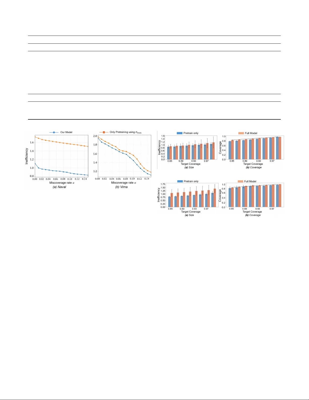
Conf ormalized Signal T emporal Logic Infer ence under Cov ariate Shift Y ixuan W ang 1 , Danyang Li 2 , Matthew Cleav eland 3 , Roberto T ron 2 , Mingyu Cai 1 Abstract —Signal T emporal Logic (STL) inference learns in- terpret able logical rules f or temporal behaviors in dynamical systems. T o ensure the correctness of learned STL formulas, recent approaches hav e incorporated conformal prediction as a statistical tool for uncertainty quantification. Howe ver , most existing methods rely on the assumption that calibration and testing data are identically distributed and exchangeable, an assumption that is frequently violated in real-world settings. This paper proposes a conf ormalized STL inference framework that explicitly addresses covariate shift between training and deployment trajectories dataset. From a technical standpoint, the approach first employs a template-free, differentiable STL inference method to learn an initial model, and subsequently refines it using a limited deployment side dataset to promote distribution alignment. T o provide validity guarantees under distribution shift, the framework estimates the likelihood ratio between training and deployment distributions and integrates it into an STL-rob ustness-based weighted conformal pr ediction scheme. Experimental results on trajectory datasets demonstrate that the proposed framework preserv es the interpretability of STL formulas while significantly improving symbolic learning reliability at deployment time. The project page can be found: https://sites.google.com/ucr .edu/confrtlics?usp=sharing. Index T erms —Formal Methods, Conf ormal Prediction, Signal T emporal Logic, T emporal Logic Inference, I . I N T RO D U C T I O N Interpretable decision models are particularly valuable in control and robotics, where learned decision rules are often used in safety-critical settings and must therefore be inspected and verified. Signal T emporal Logic (STL) provides an interpretable formal language for describing temporal beha viors of dynamical systems. It specifies temporal properties through human- readable logical formulas and equips them with a quantitative robustness semantics to measure the degree of satisfaction or violation. These properties make STL a useful foundation for learning interpretable classifiers ov er trajectories. A substantial body of prior work has studied STL inference from data. Early methods typically relied on fixed logical templates or small template families and optimized real-valued parameters using 1 Mingyu Cai and Y ixuan W ang are with Mechanical Engineering, Univ ersity of California, Riverside, CA, 92521, USA. { mingyu.cai, ywang1457 } @ucr.edu 2 Danyang Li and Roberto T ron are with Mechanical Engineering, Boston Univ ersity . { danyangl, tron } @bu.edu 3 Matthew Cleav eland is with MIT Lincoln Laboratory , Lexington, MA, 02421, USA { matthew.cleaveland@ll } @mit.edu DISTRIBUTION ST A TEMENT A. Approved for public release. Distribution is unlimited. This material is based upon work supported by the Department of the Army under Air Force Contract No. F A8702-15-D-0001 or F A8702-25- D-B002. Any opinions, findings, conclusions or recommendations expressed in this material are those of the author(s) and do not necessarily reflect the views of the Department of the Army . © 2026 Massachusetts Institute of T echnology . Deliv ered to the U.S. Government with Unlimited Rights, as defined in DF ARS Part 252.227-7013 or 7014 (Feb 2014). Notwithstanding any copyright notice, U.S. Government rights in this work are defined by DF ARS 252.227-7013 or DF ARS 252.227-7014 as detailed above. Use of this work other than as specifically authorized by the U.S. Government may violate any copyrights that exist in this work. robustness-based objectives [ 1 ], [ 2 ]. More recent approaches hav e expanded the space of learnable specifications through logic-based learning from demonstrations, and differentiable neural-symbolic frameworks that embed temporal and Boolean operators into trainable computation graphs [ 3 ], [ 4 ], [ 5 ], [ 6 ], [ 7 ], [ 8 ], [ 9 ]. These dev elopments improv e scalability and flexibility while preserving the interpretability of the learned specifications. In particular , recent differentiable STL learning approaches optimize both formula structure and parameters directly from trajectory data, providing a practical route to compact and expressi ve symbolic classifiers. Howe ver , interpretability alone is not sufficient for deploy- ment. In many control and robotics applications, a learned classifier is not only expected to be accurate, but also to quantify the reliability of the decisions. A symbolic STL formula may be human-readable, yet its predictions can still be poorly calibrated or statistically unreliable when learned from finite data. This moti vates the need for statistical correctness guarantees in addition to interpretable formula learning. Con- formal prediction (CP) provides a principled frame work for this purpose by conv erting a real-valued score into a calibrated decision rule with finite-sample coverage guarantees under exchangeability [ 10 ], [ 11 ]. In practice, split CP uses a held-out calibration set and empirical quantiles nonconformity scores, which are then used as thresholds for constructing calibrated decision rules [ 12 ], [ 13 ], [ 14 ]. CP has also been used in robotics and control to provide calibrated decision rules and uncertainty- aware safety wrappers for learning-based systems [ 15 ], [ 16 ], [ 17 ]. In previous works [ 18 ], [ 19 ], CP was integrated with dif ferentiable STL inference e.g., TLINet [ 7 ] and STLcg [ 6 ], to quantify prediction uncertainty while preserving interpretability . A further challenge is that standard CP relies on exchange- ability , meaning that the calibration data and the future test data are assumed to follo w the same distrib utional mechanism. STL formula are typically learned from trajectories collected under nominal or controlled conditions, whereas deployment trajectories may differ because of en vironmental variation, operational changes, or data-collection bias. Such cov ariate shift can substantially de grade deployment-time reliability ev en when the conditional labeling rule remains unchanged. Existing STL inference methods primarily optimize empirical performance on source-side data and do not explicitly address calibration under distribution mismatch between source-side and deployment-side distributions. Prior conformalized STL inference [ 18 ], [ 19 ], does not explicitly address mismatch among training, calibration, and deployment data. W eighted CP provides one statistical mechanism for handling such mismatch by re weighting calibration samples according to their deployment relev ance [ 20 ], [ 15 ]. As a result, we posit that in the STL setting, reliability under distribution shift should be addressed jointly at two lev els: the learned formula should adapt tow ard deployment-rele vant regions, and the final decision threshold should be calibrated in a distribution-aware manner . Our framework is more broadly compatible with dif ferentiable STL inference methods. In the sequel, we formulate the method using binary trajectory classification as a concrete instantiation. Motiv ated by this challenge, we study conformalized STL inference under cov ariate shift. Our approach starts from a differentiable STL inference model and refines the learned formula using an additional dataset that is more representati ve of deployment conditions. The refinement stage adapts the formula toward the test-time distribution through data reweight- ing [ 21 ], [ 22 ] and robustness-distrib ution regularization [ 23 ]. W e then perform weighted CP for the resulting robustness- based decision rule, so that calibration better reflects the test- time distribution. In this way , the framework jointly addresses formula adaptation and statistical calibration under distribution shift. Contributions are as follows: • W e dev elop a covariate-shift-a ware incremental learning scheme for differentiable STL inference that adapts a pretrained STL formula through STL rob ustness based distributional alignment, while maintaining both classification performance and interpretability . • T o provide statistical correctness under distribution mismatch, we extend conformalized STL inference to the covariate shift setting using weighted CP [ 20 ] with a robustness-based nonconformity score tailored to learned STL formulas. • T o improve the stability of shift alignment during learning, we introduce a distrib ution-level termination criterion that ineffecti ve learning iterations. • Experiments on trajectory datasets demonstrate that the proposed method achiev es well-calibrated inference coverage under covariate shift and reduces empirical miscoverage. I I . P R E L I M I NA R I E S W e work with trajectories of the form x = ( x 0 , . . . , x T ) , where x t ∈ R d denotes the system state at time t . A. Signal T emporal Logic Infer ence Signal T emporal Logic (STL) is a formal language for describing temporal and spatial properties of time-series data. Atomic predicates are taken to be linear inequalities of the form µ ( x t ) ≡ a ⊤ x t ≥ b, a ∈ R d , b ∈ R , which test whether a linear constraint on the state is satisfied at a giv en time. STL formula are generated from atomic predicates according to the grammar φ ::= µ   ¬ φ   φ 1 ∧ φ 2   φ 1 ∨ φ 2   ♢ [ t 1 ,t 2 ] φ   □ [ t 1 ,t 2 ] φ where ¬ , ∧ and ∨ denote Boolean negation, conjunction and disjunction, ♢ t 1 ,t 2 and □ [ t 1 ,t 2 ] are the temporal ”ev entually” and “always” operators ov er the interval [ t 1 , t 2 ] ⊆ { 0 , . . . , T } . The standard quantitati ve semantics of STL associates to each formula φ , trajectory X , and time t a real-valued robustness score ρ φ ( X, t ) ∈ R that measures the degree of satisfaction. W e denote ρ φ ( X ) := ρ φ ( X, 0) . Positi ve values indicate satisfaction, negati ve v alues indicate violation, and lar ger absolute values correspond to larger robustness margins. For atomic predicates, Boolean operators, and temporal operators, the robust semantics are defined recursively as follows: ρ µ ( X, t ) = a ⊤ x t − b (1) ρ ¬ φ ( X, t ) = − ρ φ ( X, t ) (2) ρ φ 1 ∧ φ 2 ( X, t ) = min  ρ φ 1 ( X, t ) , ρ φ 2 ( X, t )  (3) ρ φ 1 ∨ φ 2 ( X, t ) = max  ρ φ 1 ( X, t ) , ρ φ 2 ( X, t )  (4) ρ ♢ [ t 1 ,t 2 ] φ ( X, t ) = max τ ∈ [ t 1 ,t 2 ] ρ φ ( X, t + τ ) (5) ρ □ [ t 1 ,t 2 ] φ ( X, t ) = min τ ∈ [ t 1 ,t 2 ] ρ φ ( X, t + τ ) (6) STL formulas can be used as binary classifiers for trajectories through the sign of the robustness score. Giv en a labeled trajectory ( X , Y ) with Y ∈ {− 1 , +1 } , define ˆ Y ( X ) = ( +1 , ρ φ ( X ) > 0 , − 1 , otherwise (7) Thus, the product Y ρ φ ( X ) is positiv e when the robustness sign agrees with the true label and negati ve otherwise. a) Misclassification rate (MCR): For an e valuation dataset D = { ( X i , Y i ) } n i =1 , the misclassification rate (MCR) induced by φ is defined as MCR( D ; φ ) = 1 n n X i =1 1 h ˆ Y ( X i )  = Y i i Minimizing the MCR corresponds to learning an STL formula whose robustness sign aligns with the ground-truth labels. b) Differ entiable STL learning (TLINet): TLINet [ 7 ] is adopted as a differentiable STL learner for optimizing STL formulas from data. Since the 0-1 misclassification loss 1 [ Y ρ φ θ ( X ) ≤ 0] is non-dif ferentiable, optimization is performed using a smooth margin-based surrogate, namely the logistic loss, as described in Sec IV -A. B. Conformal Pr ediction Conformal Prediction (CP) [ 11 ] is a distrib ution-free proce- dure that augments the output of a fixed predicti ve model with prediction regions that enjoy finite-sample cov erage guarantees. In split CP , calibration is performed on a held-out dataset using a nonconformity score, which measures how inconsistent a labeled sample is with the model’ s decision rule. The dataset is partitioned into a training set D train , a calibration set D cal = { ( X i , Y i ) } n cal i =1 , and a test set D test , where D cal and a new test sample are exchangeable. In our shift-aware setting, the calibration data are not assumed exchangeable with the test data. Instead, weighted CP is used to approximate deployment- relev ant nonconformity score quantiles under cov ariate shift. Let A : X × Y → R denote a measurable nonconformity score function, where X is the trajectory space and Y is the label space. The nonconformity scores on the calibration set are computed as s i = A  X i , Y i ) , i = 1 , . . . , n cal . (8) For a target miscov erage level α ∈ (0 , 1) , the conformal threshold is defined as the (1 − α ) quantile of the multiset { s 1 , . . . , s n cal } . Specifically , let k = ⌈ ( n cal + 1)(1 − α ) ⌉ and define T CP := s ( k ) , where s ( k ) denotes the k -th smallest value. The resulting CP set for a test input X test ∈ X is C ( X test ) := { Y test ∈ Y : A ( X test , Y test ) ≤ T CP } Under the exchangeability assumption, the CP guarantee yields P ( Y test ∈ C ( X test )) ≥ 1 − α (9) I I I . P RO B L E M F O R M U L A T I O N W e consider the problem of binary classification of system trajectories using STL. Let φ θ denote an STL formula learned by a differentiable STL inference method, where θ collects the learnable formula parameters, such as predicate and temporal parameters. The induced robustness score ρ φ θ ( X ) is used to define the binary classification. a) Data distributions and covariate shift: Follo wing the distribution-shift setting described in the introduction, let P train denote the nominal training distribution and P dep denote the deployment distribution. W e consider a cov ariate shift setting in which the conditional labeling rule remains in variant while the marginal distribution over trajectories changes. Assumption 1 (Cov ariate Shift under STL Semantics) . W e assume P train ( Y | X ) = P dep ( Y | X ) , P train ( X )  = P dep ( X ) This assumption is natural in our setting because labels are defined by STL satisfaction, which depends only on the trajectory and the specification, and is therefore in variant to operating conditions. b) Data partitioning: W e consider three mutually disjoint datasets. A core training set D train ∼ P train is used to learn an initial STL formula and define task semantics. Because it is collected under nominal or conserv ative conditions, it may not adequately cover the range of trajectories encountered at deployment. W e assume access to a limited deployment-side dataset D dep that captures beha viors underrepresented in D train . Although D dep is only a partial and potentially biased sample from P dep , it provides information about regions likely to arise at test time and is incorporated only through distribution- aware objectives, without altering the labeling rule. Finally , a separate calibration set D cal ∼ P train is reserved exclusi vely for weighted conformal calibration of the robustness-based decision rule [ 11 ], [ 17 ]. Since D cal is drawn from P train whereas deployment-time test trajectories follow P dep , standard calibration is no longer distribution-matched. W e therefore use importance weighting to make calibration better reflect the target deployment distribution. c) Problem F ormulation: Giv en D train , D dep , and D cal as defined above, the objectiv e is to learn φ θ . For a θ , the corresponding prediction set is induced by the calibration rule and is denoted by C θ ( · ) . The resulting STL decision rule should achie ve both low misclassification and reliable coverage under the deployment distribution: min θ MCR P dep ( φ θ ) := E ( X,Y ) ∼ P dep [ 1 [ Y ρ φ θ ( X ) ≤ 0]] s.t. P ( X,Y ) ∼ P dep ( Y ∈ C θ ( X )) ≥ 1 − α Fig. 1: Pipeline of proposed shift-aware conformal STL framew ork under co variate shift. The framew ork consists of four sequential stages integrating STL formula learning, distribution alignment, and weighted conformal calibration. Remark 1 . Challenges and Motivations: If the cov ariate shift is ignored, an STL formula learned only from D train may ov erfit regions of the trajectory space that are well represented during training but less relev ant at deployment, leading to degraded classification performance and miscalibration under P dep . This can be effecti ve when D dep is suf ficiently large and representativ e, but in practice the av ailable deployment-side data is often limited and distributionally mismatched relati ve to D train , making nai ve retraining statistically unstable. Our approach instead uses the STL formula learned from D train as a warm start and incorporates D dep through distribution-a ware objectiv es that steer the learned robustness scores toward regions more relev ant to deployment. T o assess how informative the deployment-side data is, we monitor an effecti ve sample size diagnostic deri ved from density-ratio weights. This quantity reflects the concentration of the weights and indicates whether further refinement additional refinement is likely to materially improve deployment alignment. I V . C O N F O R M A L I Z E D A C T I V E S T L I N F E R E N C E U N D E R C OV A R I A T E S H I F T In Section IV -A , we present a shift-aware STL framew ork that learns a formula from training data and adapts it using deployment-proxy data. Section IV -B establishes correctness guarantees under distribution shift. The overall pipline is summerized in Fig. 1 A. STL Infer ence Adaptation The frame work builds on TLINet [ 7 ] as a dif ferentiable, template-free backbone for learning STL formulas from labeled trajectories, enabling gradient-based optimization and yielding interpretable, parameterized STL specifications. T raining is performed by minimizing a margin-based surrogate loss applied to the signed robustness value Y ρ φ θ ( X ) . Follo wing TLINet, the logistic loss is used: ℓ ( Y ρ φ θ ( X )) = log(1 + exp( − Y ρ φ θ ( X ))) Giv en a core training dataset D train = { ( X i , Y i ) } n c i =1 , the nominal STL formula is obtained by minimizing the empirical surrogate loss L train ( θ ) = 1 n c X ( X,Y ) ∈ D train ℓ ( Y ρ φ θ ( X )) Let θ 0 denote a minimizer of L train , and φ θ 0 the corre- sponding STL formula learned from D train . The parameter θ 0 defines the nominal STL formula φ θ 0 learned from the training dataset D train . This formula serves as a warm-start initialization for the subsequent shift-aware adaptation stage, and provides the semantic structure of the STL specification. The adaptation stage further refines them using deployment- side data D dep tow ard deployment-rele vant trajectory regions through the distribution-a ware objectiv es introduced below . a) Density-Ratio W eighting on the Alignment Set: As defined in Section III, the learning setting assumes a cov ariate shift between training and deployment trajectories. For a trajectory X ∈ X , the ideal importance weight is the density ratio that exactly reweights expectations from the training distribution to the deployment distrib ution: ω ⋆ ( X ) := p dep ( X ) p train ( X ) (10) where p train and p dep denote the underlying marginal densities of trajectories under training and deployment distributions, respectiv ely . Direct estimation of ω ⋆ ( X ) is generally difficult without strong parametric assumptions. W e therefore approximate it using a k -nearest-neighbor (kNN) density-ratio estimator in an embedding space [ 24 ], which provides a simple nonparametric approximation based on local sample density . Other density- ratio estimators, such as kernel mean matching (KMM), KLIEP , and uLSIF , could also be used [ 25 ]. The intuition is that, in a p - dimensional embedding space, the local sample density around X is approximately in versely proportional to the volume of its kNN neighborhood, and hence to r k ( X ; S ) p . Therefore, the ratio of kNN radii provides a local approximation to the density ratio between the deployment and training distributions. T o instantiate this estimator, let f : X → R p denote a fixed embedding. For a reference set S , we define the kNN radius of X as r k ( X ; S ) = ∥ f ( X ) − f ( X ( k ) ) ∥ 2 where X ( k ) ∈ S is the k -th nearest neighbor of X . The unnormalized kNN density-ratio weight is then given by ˆ ω ( X ) =  r k ( X ; D train ) r k ( X ; D dep )  p T o improv e numerical stability , we normalize the ra w weights to have unit empirical mean over D dep and clip them to a fixed range: ˜ ω ( X ) = ˆ ω ( X ) 1 | D dep | P X ′ ∈ D dep ˆ ω ( X ′ ) (11) ω ( X ) = min { max { ˜ ω ( X ) , ω min } ω max } (12) Hence, ω ( X ) is used as a practical approximation to the ideal density-ratio weight ω ⋆ ( X ) . Although not exact, it captures relati ve distributional differences between P train and P dep and emphasizes trajectories more relev ant to deployment. Lemma 1. Under Assumption 1, assume that P dep is absolutely continuous with r espect to P train over X . Then, with ideal density-ratio weight ω ⋆ ( X ) , for any measurable function h : X × {− 1 , +1 } → R with finite expectation, we have E ( X,Y ) ∼ P dep [ h ( X, Y )] = E ( X,Y ) ∼ P train [ ω ⋆ ( X ) h ( X, Y )] Pr oof. By the law of total expectation under P dep , E P dep [ h ( X, Y )] = Z X X y ∈{− 1 , +1 } h ( x, y ) p dep ( y | x ) p dep ( x ) dx Using p dep ( x ) = ω ⋆ ( x ) p train ( x ) , we obtain E P dep [ h ( X, Y )] = Z X X y ∈{− 1 , +1 } h ( x, y ) ω ⋆ ( x ) p train ( y | x ) p train ( x ) dx = E P train [ ω ⋆ ( X ) h ( X, Y )] Proposition 1. Under covariate shift, consider the expected misclassification rate under the deployment distribution P dep . F or any fixed STL formula φ θ , the misclassification rate under the deployment distribution can be written as E ( X,Y ) ∼ P dep  1 { Y ρ φ θ ( X ) ≤ 0 }  = E ( X,Y ) ∼ P train  ω ⋆ ( X ) 1 { Y ρ φ θ ( X ) ≤ 0 }  In practice, ω ⋆ ( X ) is r eplaced by its kNN-based appr oximation ω ( X ) . Pr oof. This proposition is a special case of Lemma 1 with h ( X, Y ) = 1 { Y ρ φ 0 ( X ) ≤ 0 } . Proposition 1 motiv ates a deployment-time learning objectiv e that combines the nominal training loss on D train with a weighted loss on D dep . L train ( θ ) = 1 | D train | X ( X,Y ) ∈ D train ℓ ( Y ρ φ θ ( X )) + 1 | D dep | X ( X,Y ) ∈ D dep ω ( X ) ℓ ( Y ρ φ θ ( X )) The first term preserves the nominal STL semantics learned from D train , while the second term emphasizes deployment- relev ant trajectories through density-ratio weighting. Howe ver , these two terms alone are not sufficient. In practice, the estimated density-ratio weights can be highly non-uniform, so direct optimization of the weighted term may lead to unstable updates and may distort the robustness structure learned from D train [ 20 ]. T o stabilize refinement and further adapt the learned STL rule at the distribution le vel, we add a robustness- distribution regularizer based on the Jensen–R ´ enyi div ergence (JRD) [26]. b) Regularization of Rob ustness-V alue Distributions via J ensen–R ´ enyi Diverg ence: The JRD is adopted to compare the empirical robustness distributions induced on D train and D dep . As a symmetric di vergence between probability measures, it provides a distribution-le vel adaptation term that encourages the learned robustness values to remain aligned across the source and deployment-side data. Other distributional discrepancies, e.g., Jensen–Shannon di vergence [27], could also be used. Definition 1. For a giv en parameter θ , define the empirical robustness distributions induced by the training set and the deployment set as ˆ P θ train := 1 | D train | X ( X,Y ) ∈ D train δ ρ φ θ ( X ) ˆ P θ dep := 1 | D dep | X X ∈ D dep δ ρ φ θ ( X ) (13) where δ ρ φ θ ( X ) denotes the unit point mass located at the robustness value ρ φ θ ( X ) . The following proposition shows that this regularizer yields an explicit bound on the resulting robustness-distribution mismatch. Proposition 2. Consider the r egularized training objective L ( θ ) = L train ( θ ) + λ JRD JRD  ˆ P θ train , ˆ P θ dep  wher e λ JRD > 0 is a r e gularization parameter contr olling the str ength of the r obustness-distrib ution alignment penalty . Let θ ⋆ be a minimizer of L , and let θ train be a minimizer of the unr e gularized training loss L train . Then JRD  ˆ P θ ⋆ train , ˆ P θ ⋆ dep  ≤ L train ( θ train ) − L train ( θ ⋆ ) λ JRD + JRD  ˆ P θ train train , ˆ P θ train dep  Pr oof. By optimality of θ ⋆ , we hav e L ( θ ⋆ ) ≤ L ( θ train ) . Rearranging terms yields λ JRD JRD  ˆ P θ ⋆ train , ˆ P θ ⋆ dep  ≤ L train ( θ train ) − L train ( θ ⋆ ) + λ JRD JRD  ˆ P θ train train , ˆ P θ train dep  which implies the stated bound. Although the practical density-ratio weights are clipped to improv e numerical stability , clipping alone does not directly control distribution-le vel drift in the induced robustness values. W e therefore refine the pretrained STL formula by minimizing the following unified shift-aware objectiv e: L ( θ ) = 1 | D train | X ( X,Y ) ∈ D train ℓ ( Y ρ φ θ ( X )) + 1 | D dep | X ( X,Y ) ∈ D dep ω ( X ) ℓ ( Y ρ φ θ ( X )) + λ JRD JRD  ˆ P θ train , ˆ P θ dep  (14) where ω ( X ) denotes the density-ratio weight, and λ JRD > 0 is a regularization parameter . B. W eighted Conformalized STL Infer ence This section aims to provide correctness guarantees using CP for the learned STL formulas. The general nonconformity score in Section II-B is specialized to the rob ustness-based form for binary classification. A ( X, Y ) = S θ ( X, Y ) := − Y ρ φ θ ( X ) , (15) where larger v alues of S θ indicates stronger disagreement with label Y . This choice is simple and compatible with our prior formulation [ 19 ]. More importantly , it yields a unified decision statistic: the same signed robustness margin governs STL training, binary classification, and CP . Under cov ariate shift, calibration and deployment-time test samples are generally not exchangeable. W e therefore adopt weighted CP [ 20 ], where the calibration nonconformity scores are re weighted according to the density-ratio weights introduced in Section IV -A . The nonconformati vity scores on D cal are defined as s i := S θ ( X i , Y i ) , i = 1 , . . . , n cal (16) The weighted empirical cumulativ e distribution of the calibration nonconformity scores is defined as ˆ F w ( t ) := P n i =1 ω ( X ) 1 { s i ≤ t } P n i =1 ω ( X ) (17) The weighted conformal threshold is then taken as the (1 − α ) - quantile of this weighted empirical distribution: T wcp := inf n t ∈ R : ˆ F w ( t ) ≥ 1 − α o (18) Accordingly , the weighted CP set is defined by C ( X ) = { Y ∈ {− 1 , +1 } : S θ ( X, Y ) ≤ T wcp } . (19) Under Assumption 1, and using the ideal density-ratio weight ω ⋆ ( X ) defined in Section IV -A , the prediction set C ( X ) is a direct specialization of the weighted conformal construction under covariate shift in [20] with coverage guarantees, i.e., P ( X,Y ) ∼ P dep ( Y ∈ C ( X )) ≥ 1 − α (20) In practice, howe ver , highly non-uniform weights may reduce the effecti ve number of weighted samples and increase the variability of weighted empirical estimates. W e can quantify this effect by adopting the effecti ve sample size (ESS) [28]. ESS( D ) =  P X ∈ D ω ( X )  2 P X ∈ D ω ( X ) 2 with the normalized form ESS( D ) / | D | ∈ (0 , 1] . The following result formalizes the relation between weight concentration and the conditional variability of weighted empirical estimates. Proposition 3. Let { Z i } n i =1 be i.i.d. fr om a distribution Q and let { w i } n i =1 be nonne gative weights with normalized weights ¯ w i := w i / P n j =1 w j . F or any measurable g with g ( z ) ∈ [ − 1 , 1] for all z , define ˆ µ w ( g ) := n X i =1 ¯ w i g ( Z i ) Then, conditional on the weights ( w 1 , . . . , w n ) , V ar  ˆ µ w ( g ) | w 1: n  ≤ n X i =1 ¯ w 2 i = 1 ESS , This bound sho ws that the conditional variability of a weighted empirical estimate is controlled by 1 / ESS . In particu- lar , smaller ESS yields a larger upper bound on the conditional variance, indicating reduced stability when the weights are highly concentrated. Pr oof. The quantity ˆ µ w ( g ) is a weighted average of inde- pendent variables g ( Z 1 ) , . . . , g ( Z n ) , each bounded in [ − 1 , 1] . Conditional on the weights, the variance is therefore bounded by the sum of squared normalized weights. Since | g | ≤ 1 , V ar[ g ( Z i )] ≤ 1 . Independence yields V ar " n X i =1 ¯ w i g ( Z i ) # = n X i =1 ¯ w 2 i V ar[ g ( Z i )] ≤ n X i =1 ¯ w 2 i Finally , n X i =1 ¯ w 2 i = P n i =1 w 2 i ( P n i =1 w i ) 2 = 1 ESS As a result, we can use ESS as a learning termination crite- rion of balancing the ov erfitting and maintaining the effecti ve number of calibration samples for the distrib utional alignment during shift iterati ve refinement procedure. In particular, let ESS ( t ) denote the effecti ve sample size at iteration t . learning prcoess in Section IV -A is terminated when      ESS ( t ) n − ESS ( t − 1) n      ≤ ε where n is the number of calibration samples and ε > 0 is a tolerance parameter . This criterion indicates that further updates no longer substantially change the effecti ve distribution alignments. V . E X P E R I M E N TA L R E S U L T S W e e valuate the proposed conformalized STL inference framew ork on three trajectory datasets with distinct distri- butional characteristics under covariate shift. All experiments were conducted on a Linux workstation equipped with an Intel Core i9-13900KF CPU (24 cores, 32 threads). The objectiv es of the experiments are threefold: • T o assess the classification performance of the refined STL classifier compared to nominal TLINet training; • T o ev aluate the behavior of CP under distribution shift; • T o examine the efficienc y-cov erage tradeoff between standard CP and weighted CP . A. Evaluation Metrics For a target miscoverage level α , the conformal predictor aims to achiev e a coverage lev el of 1 − α . In experiments we report the empirical coverage, defined as Cov erage = 1 n n X i =1 1 { Y i ∈ C ( X i ) } (21) (a) VIMA simulated environment (b) V ima Dataset (c) Nav al Dataset (d) Motion Planning Dataset Fig. 2: Schematic Diagram of the Dataset which estimates the probability that the prediction set contains the true label under the test distribution. T o quantify the efficienc y of the prediction sets, we report the average prediction set size, referred to as inefficienc y: Inefficienc y = 1 n n X i =1 | C ( X i ) | (22) This metric measures the av erage size of prediction sets, where smaller values correspond to more compact predictions. In the binary classification setting considered here, the prediction set C ( X ) is defined in Section II-B has cardinality in { 0 , 1 , 2 } . A singleton set corresponds to a confident prediction, a two-label set indicates ambiguity , and an empty set indicates that neither label satisfies the acceptance condition. B. Datasets Dataset 1: Naval Surveillance: The Naval Surveillance dataset consists of labeled time-series trajectories deriv ed from a marine propulsion system benchmark. Each trajectory is a multiv ariate signal X ∈ R d × T , and the task is binary classification of normal versus anomalous operational behavior . Dataset 2: Place a block into a basket without violating the safety constraint. This task requires the robot to transport a target block into a designated basket region while keeping the trajectory within the basket boundary marked by tape. C. Baseline Comparison W e compare our frame work with sev eral baseline classifiers on the considered trajectory datasets: TLINet, a differentiable STL inference model; LSTM/RNN, a recurrent neural-network baseline for sequence classification [ 29 ]; BCDT , a boosted classification-tree method [ 30 ], [ 31 ]; DT , a standard decision tree [ 32 ]; and DA G, a directed-acyclic-graph-based temporal classifier [ 33 ], [ 34 ]. These methods serve as reference baselines for classification performance. Neural baselines such as LSTM T ABLE I: Classification results of our method and baseline methods on trajectory datasets. Method MCR for P train MCR for P dep T ime(s) STL formula Nav al Dataset Ours 1.25 0.07 16 ♢ [25 , 26] ( x ≤ 38 . 6) ∧ □ [11 , 12] ( y ≥ 24 . 1) TLINet 1.25 0.05 38 ♢ [55 , 60] ( x < 25 . 89) ∧ □ [0 , 16] ( y > 23 . 77) LSTM/RNN 0.01 0.025 19 N/A BCDT 0.0100 N/R 1996 ♢ [28 , 53] ( x < 30 . 85) ∧ □ [2 , 26] ( y > 21 . 31) ∧ ( x > 11 . 10) DT 0.0195 N/R 140 ¬ ( ♢ [38 , 53] ( x > 20 . 1) ∧ ♢ [12 , 37] ( x > 43 . 2)) ∨ ( ♢ [38 , 53] ( x > 20 . 1) ∧ ¬ ♢ [20 , 59] ( y > 32 . 2)) ∨ ( ♢ [38 , 53] ( x > 20 . 1) ∧ ♢ [20 , 59] ( y > 32 . 2) ∧ □ [14 , 60] ( y > 30 . 1)) D A G 0.0885 N/R 996 ♢ [0 , 33] ( □ [18 , 23] ( y > 19 . 88) ∧ □ [9 , 30] ( x < 34 . 08)) VIMA Dataset Ours 8.55 0.015 15 □ [17 , 19] ((88 . 62 < x < 152 . 21) ∧ (45 . 47 < y < 89 . 73)) TLINet 8.55 0.0125 45 □ [17 , 19] ((89 . 86 < x < 147 . 14) ∧ (59 . 64 < y < 89 . 97)) LSTM/RNN 8.30 0.08 23 N/A Fig. 3: W eighted CP with Covariate Shift can be further adapted with additional data, whereas the remaining non-neural baselines do not naturally admit the same gradient-based refinement mechanism as our framew ork and typically require retraining instead. T able I report the MCR, training time, and the learned STL formulas for all compared methods. Across the ev aluated datasets, models trained only on source-side data degrade under the deployment distribution, which is consistent with covariate shift. Our framew ork reduces this degradation by refining the core trained STL formula with deployment-side data and remains close to the oracle TLINet trained directly on P dep . Compared with the neural and tree-based baselines, it achiev es competiti ve or better classification performance while retaining an explicit STL formula. The reported training times sho w that the additional refinement stage remains computationally practical. D. Ablation Study a) STL Classification: T able I isolates the effect of the shift-aware refinement stage. T raining only on D train leads to degraded performance under P dep , while incorporating P dep substantially reduces the MCR across datasets. b) W eighted Conformal Pr ediction under Covariate Shift: Figure 3 compares weighted CP applied to the refined STL classifier with the same procedure applied to a model trained without shift-aware retraining. In both cases, density-ratio weighting is used during calibration. On the Nav al dataset, the refined model yields substantially smaller prediction set sizes across all miscoverage lev els. The (a) Nav al Dataset (b) Motion Planning Dataset Fig. 4: Comparison across datasets with weighted CP . gap between the two curves remains consistent, indicating that shift aware retraining improves the alignment between the learned robustness scores and the deployment distribution. As a result, fewer candidate labels are required to maintain the same cov erage level. A similar trend is observed on VIMA. Although the difference is less pronounced than in Nav al, the refined model consistently achiev es lo wer inefficiency across the range of target miscoverage lev els. This suggests that incorporating D dep during training reduces the impact of mar ginal distribution mismatch on the calibration score distribution. Overall, these results indicate that shift-aware refinement enhances the effecti veness of weighted CP by improving the distributional alignment of rob ustness scores under deployment conditions. c) Effect of Shift-aware Refinement on Conformal Pr edic- tion: Figures 4 further examine how shift-aware refinement af fects CP . On both datasets, the refined model yields prediction sets whose av erage size is closer to one at comparable target cov erage levels, indicating better alignment between the learned robustness scores and the deployment distribution. At the same time, empirical co verage remains closer to the target le vel across settings. Fig. 5: Comparison between weighted CP and Standard CP using our method in dif ferent dataset. d) W eighted vs. Standard Conformal Prediction: Figure 5 compares weighted CP and standard CP in terms of empirical cov erage–inefficiency trade-of fs on the Na val and VIMA datasets. Across both datasets, the two methods yield closely matched curves, indicating that density-ratio reweighting has only a minor ef fect on the conformal quantile in the current setting. This suggests that the calibration and test score distributions are already reasonably aligned after refinement. V I . C O N C L U S I O N W e studied STL-based trajectory classification under cov ari- ate shift and proposed a shift-aw are STL inference framework that refines a learned STL formula using deployment-time data. The method combines TLINet pretraining with a refinement stage that improv es the alignment between the learned robust- ness scores and the deployment distribution. In addition, CP is incorporated to quantify prediction uncertainty while main- taining statistical coverage guarantees. Experimental results on multiple trajectory datasets show that the proposed frame work improv es classification performance under distribution shift while preserving the interpretability of STL-based decision rules. Future work includes extending the approach to multi- class STL inference and in vestigating more advanced shift- adaptation strategies. R E F E R E N C E S [1] E. Asarin, A. Donz ´ e, O. Maler, and D. Nickovic, “Parametric identifi- cation of temporal properties, ” in International Conference on Runtime V erification . Springer, 2011, pp. 147–160. [2] B. Hoxha, A. Dokhanchi, and G. Fainekos, “Mining parametric temporal logic properties in model-based design for cyber -physical systems, ” International Journal on Software T ools for T ec hnology T ransfer , vol. 20, no. 1, pp. 79–93, 2018. [3] E. Bartocci, C. Mateis, E. Nesterini, and D. Nickovic, “Survey on mining signal temporal logic specifications, ” Information and Computation , vol. 289, p. 104957, 2022. [4] G. Bombara and C. Belta, “Offline and online learning of signal temporal logic formulae using decision trees, ” ACM T ransactions on Cyber- Physical Systems , vol. 5, no. 3, pp. 1–23, 2021. [5] C. Y oo and C. Belta, “Rich time series classification using temporal logic, ” in Robotics: Science and Systems , 2017. [6] K. Leung, N. Ar ´ echiga, and M. Pav one, “Backpropagation through signal temporal logic specifications: Infusing logical structure into gradient- based methods, ” The International Journal of Robotics Researc h , vol. 42, no. 6, pp. 356–370, 2023. [7] D. Li, M. Cai, C.-I. V asile, and R. Tron, “Tlinet: Differentiable neural network temporal logic inference, ” 2024. [Online]. A vailable: https://arxiv .org/abs/2405.06670 [8] ——, “Learning signal temporal logic through neural network for interpretable classification, ” in 2023 American Contr ol Conference (ACC) . IEEE, 2023, pp. 1907–1914. [9] R. Y an, Z. Xu, and A. Julius, “Swarm signal temporal logic inference for swarm behavior analysis, ” IEEE Robotics and Automation Letters , vol. 4, no. 3, pp. 3021–3028, 2019. [10] V . V o vk, A. Gammerman, and G. Shafer, Algorithmic learning in a random world . Springer , 2005. [11] A. N. Angelopoulos and S. Bates, “ A gentle introduction to conformal prediction and distribution-free uncertainty quantification, ” arXiv pr eprint arXiv:2107.07511 , 2021. [12] H. Papadopoulos, Inductive conformal prediction: Theory and application to neural networks . INTECH Open Access Publisher Rijeka, 2008. [13] J. Lei, M. G’Sell, A. Rinaldo, R. J. T ibshirani, and L. W asserman, “Distribution-free predictive inference for regression, ” Journal of the American Statistical Association , vol. 113, no. 523, pp. 1094–1111, 2018. [14] Y . Romano, E. Patterson, and E. Candes, “Conformalized quantile regression, ” Advances in neural information pr ocessing systems , vol. 32, 2019. [15] A. Dixit, L. Lindemann, S. X. W ei, M. Cleaveland, G. J. Pappas, and J. W . Burdick, “ Adapti ve conformal prediction for motion planning among dynamic agents, ” in Learning for Dynamics and Control Conference . PMLR, 2023, pp. 300–314. [16] K. Liang, L. Luo, Y . W ang, M. Cai, and C. I. V asile, “Time-aw are motion planning in dynamic en vironments with conformal prediction, ” Learning for Decision and Contr ol (L4DC) , 2026. [17] L. Lindemann, M. Cleaveland, G. Shim, and G. J. Pappas, “Safe planning in dynamic environments using conformal prediction, ” IEEE Robotics and Automation Letters , vol. 8, no. 8, pp. 5116–5123, 2023. [18] E. Soroka, R. Sinha, and S. Lall, “Learning temporal logic predicates from data with statistical guarantees, ” arXiv pr eprint arXiv:2406.10449 , 2024. [19] D. Li, Y . W ang, M. Cleav eland, M. Cai, and R. T ron, “Conformal prediction for signal temporal logic inference, ” ArXiv , vol. abs/2509.25473, 2025. [Online]. A vailable: https: //api.semanticscholar .org/CorpusID:281682043 [20] R. J. T ibshirani, R. Foygel Ba rber, E. Candes, and A. Ramdas, “Conformal prediction under covariate shift, ” Advances in neural information pr ocessing systems , vol. 32, 2019. [21] H. Shimodaira, “Improving predictive inference under covariate shift by weighting the log-likelihood function, ” Journal of statistical planning and infer ence , vol. 90, no. 2, pp. 227–244, 2000. [22] D. O. Loftsgaarden and C. P . Quesenberry , “ A nonparametric estimate of a multiv ariate density function, ” The Annals of Mathematical Statistics , vol. 36, no. 3, pp. 1049–1051, 1965. [23] A. B. Hamza, “Jensen-rhyi diver gence measure: Theoretical and compu- tational perspectiv es, ” in IEEE Int. Symp. Inf. Theory , 2003. [24] P . Zhao and L. Lai, “ Analysis of knn density estimation, ” IEEE T ransactions on Information Theory , vol. 68, no. 12, pp. 7971–7995, 2022. [25] M. Sugiyama, T . Suzuki, and T . Kanamori, Density ratio estimation in machine learning . Cambridge Univ ersity Press, 2012. [26] L. G. S. Giraldo and J. C. Principe, “Information theoretic learning with infinitely divisible kernels, ” arXiv pr eprint arXiv:1301.3551 , 2013. [27] C. Shui, Q. Chen, J. W en, F . Zhou, C. Gagn ´ e, and B. W ang, “ A novel domain adaptation theory with jensen–shannon div ergence, ” Knowledge- Based Systems , vol. 257, p. 109808, 2022. [28] J. Qui ˜ nonero-Candela, M. Sugiyama, A. Schwaighofer, and N. D. Lawrence, Covariate Shift by Kernel Mean Matching , 2009, pp. 131–160. [29] S. Hochreiter and J. Schmidhuber , “Long short-term memory , ” Neural computation , vol. 9, no. 8, pp. 1735–1780, 1997. [30] J. H. Friedman, “Greedy function approximation: a gradient boosting machine, ” Annals of statistics , pp. 1189–1232, 2001. [31] E. Aasi, C. I. V asile, M. Bahreinian, and C. Belta, “Classification of time- series data using boosted decision trees, ” in 2022 IEEE/RSJ International Confer ence on Intelligent Robots and Systems (IR OS) . IEEE, 2022, pp. 1263–1268. [32] L. Breiman, J. Friedman, R. A. Olshen, and C. J. Stone, Classification and r egr ession tr ees . Chapman and Hall/CRC, 2017. [33] J. Platt, N. Cristianini, and J. Shawe-T aylor , “Large margin dags for multiclass classification, ” Advances in neural information pr ocessing systems , vol. 12, 1999. [34] Z. K ong, A. Jones, and C. Belta, “T emporal logics for learning and detection of anomalous behavior , ” IEEE T ransactions on Automatic Contr ol , vol. 62, no. 3, pp. 1210–1222, 2016.