Energy-Gain Control of Time-Varying Systems: Receding Horizon Approximation

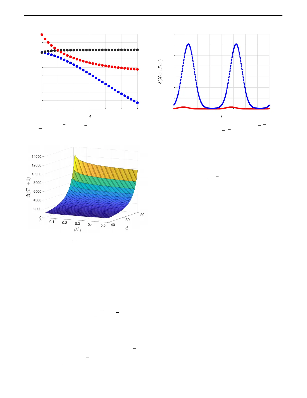
1 Energy-Gain Control of Time-V ar ying Systems: Receding Hor iz on Appro ximation Jintao Sun and Michael Cantoni Abstract — Sta n dard formulations of prescrib e d worst- case disturb ance en ergy-gain control policie s for linea r time-varyin g systems depend on all forward model data . I n discrete time, this depend e nce arise s through a b a ckward Riccati recursion. Th is a rticle is a b out the infinite- horizon ℓ 2 gain performance of state f eedba ck p olicies with only finite recedin g-horizon preview of the model parameters. The proposed synthesis of controllers s ubject to su ch a constra i nt leverages the strict c o ntraction of lifted Riccati operators under uni form co n trollability and ob s ervabilit y . The main approximation re sult is a su f ficient number of preview steps for the incurred performance loss to remain below any set toleranc e, relati ve to the basel ine gain bound of the asso ciated infinite-previ ew c ontroller . Aspe cts of the result are explored in a numerical example . Index T erms — Finite preview , infinite-h orizon perfor- mance , non-sta tionary systems , Ric cati cont ra ction I . I N T R O D U C T I O N The synthe sis of feedback con trollers for linear time-varying systems again st infinite- horizon quadratic perf ormance cr iteria has a long history [1 ]–[5]. Generally , th e standard fo rmulations are somewhat impractical, as t he contr ol p olicies d e pend on all future time-varying parameters. In th e discrete-tim e setting of this article, th e stabilizing solution of a backward Riccati recursion enc o des th is depend ence [6 ]–[9]. In p eriodic settings, inc luding the time -in variant case, a vail- ability of th e m odel data acr oss one perio d suffices to ob tain the infinite-hor izon so lution of the backward re c ursion v ia a fin ite- dimensional algeb raic Riccati equation [ 1 0]–[13 ]. In more gen e ral tim e -varying settings, an infinite- horizon lif ting, giv en all m odel data, also leads to algebra ic character ization of the solution [1 4]–[16 ]. Howev er , the p ractical conc e rn of computatio n r e mains a challenge unless a finite stru cture un- derlies the param eter variation, e.g ., perio d icity [16 ], or m ore general switching within a fin ite set [17]. Furtherm ore, infinite- horizon lifting would b e infeasible in sup ervisory h ierarchies in volving online r oll-out of finite-ho rizon plans th at de termine the m odel data relev ant fo r low-le vel con trol. This article concerns state f eedback c o ntroller synthesis subject to finite receding -horizon previe w of the time-varying Funded in par t by the A ustralian Research Council (Grant Number : DP210103272) and a Melbourne Research Scholarship . J . Sun was a student with the Depar tment of Electrical and Electronic Engineering, The Uni versity of Melbou r ne, VIC 3010, Australia. E-mail: jintaos@alumni .unimelb.edu.au M. Cantoni is with the Depar tment of Electrical and Electronic Engi- neering, The University of Melbourne, VIC 3010, A ustralia. Correspond- ing author . E-mail: cantoni@ unimelb.edu.au model d ata without previe w of the d isturbance. The goal is to ensure that the closed- loop infinite-ho rizon energy gain does n ot exceed a specified worst-case boun d. Th e p roposed approa c h in volves approximation of the standard infinite- previe w for mulation to within desired tolerance, via a Riccati contraction proper ty that ho ld s under unifo rm con trollability and ob servability and an associated finite- horizon lifting. Re- lated work on the disturbanc e -free optimal linear quadr atic regulator c a n be found in [18], [19, Ch. 4]. T o enable furth er elab o ration of the contribution, th e stan- dard form ulation of state feedback ℓ 2 gain contro llers with infinite-hor izon p r e view of the model data is recalled in Section I-A. This provides context fo r Sectio n I -B, whe re the pro posed finite reced in g-horizo n synthesis of suc h co n- trol po licies is ou tlined. Relevant literature is d iscussed in Section I-C, inclu ding well-k nown work on m odel p redictive control, and more recen t work on optimal regret, whic h b y contrast f o cuses o n perf o rmance loss relative to a po licy with non-ca u sal preview of the disturbanc e . The main te c h nical developments are map ped out in Section I -D. A. Basic notation and probl em formulation N and R den ote the natural and real num bers, N 0 := { 0 } ∪ N , and R >θ := { ϑ ∈ R : ϑ > θ } . R n denotes the space of vectors with n ∈ N real co -ordinates, and R n × m the space of matrices with n ∈ N rows and m ∈ N c o lumns of real en tries. The identity matrix is I n ∈ R n × n , all en tr ies of 0 m,n ∈ R m × n are zero, X ′ ∈ R m × n is the transpose of X ∈ R n × m , an d for non-sing ular Y ∈ R n × n , the in verse is Y − 1 ∈ R n × n . Giv en the sets o f symmetr ic matrices S n := { Z ∈ R n × n | Z = Z ′ } , S n + := { Z ∈ S n | ( ∀ v ∈ R n ) v ′ Z v ≥ 0 } , an d S n ++ := { Z ∈ S n | ( ∀ v ∈ R n ) v ′ Z v > 0 } , Y  Z m eans ( Z − Y ) ∈ S n + , and Y ≺ Z mea n s ( Z − Y ) ∈ S n ++ . For Z ∈ S n + , the matrix square root is Z 1 / 2 ∈ S n + . F or Y ∈ S n , λ min ( Y ) and λ max ( Y ) denote minim u m an d maximu m eig e n value. Consider the linear time-varying system x t +1 = A t x t + B t u t + w t , t ∈ N 0 , (1) with in itial state x 0 = 0 ∈ R n , co ntrol an d distu r bance inputs u t ∈ R m and w t ∈ R n , resp ecti vely , and per formance outpu t z t =  Q 1 / 2 t 0 n,m  ′ x t +  0 m,n R 1 / 2 t  ′ u t , (2) where A t ∈ R n × n , B t ∈ R n × m , Q t ∈ S n + , and R t ∈ S m ++ . Assumption 1: Th e m odel data A t , B t , Q t , R t and the in - verses A − 1 t , R − 1 t are u niformly boun ded acro ss t ∈ N 0 . 2 Note that A t is non - singular wh e nev er the model arises f rom discretization. He r e it en a bles direct access to key results o n Riccati operato r contra ction [20]. Generalizing to singular A t (e.g., see [21]) is beyond the curren t scope. Assumption 2 : The system ( Q 1 / 2 t , A t , B t ) t ∈ N 0 is un iformly observable a n d contro llable in the following sense [ 7]: ( ∃ d ∈ N ) ( ∃ c ∈ R > 0 ) ( ∀ t ∈ N 0 ) t + d − 1 X s = t Φ ′ s,t Q s Φ s,t !  c I n  t + d − 1 X s = t Φ s,t B s B ′ s Φ ′ s,t ! , where Φ t,t := I n , an d Φ s,t := A s − 1 · . . . · A t for s > t . While infinite-preview state feedback controllers with energy-gain guarantees exist under un iform stabilizability and detectability , Assump tion 2 play s a ro le in the Riccati contrac- tion b ased synth esis of fin ite rece ding-ho r izon app roximation s, as elabo rated in Section s II and III-A . The object of energy- gain control is to find a po licy f or u = ( u t ) t ∈ N 0 such th at the resulting map fro m the disturb a n ce input w = ( w t ) t ∈ N 0 to the perfo rmance output z = ( z t ) t ∈ N 0 is inpu t-output stable over the space of finite energy signals ℓ 2 := { w = ( w t ) t ∈ N 0 | k w k 2 2 := P t ∈ N 0 w ′ t w t < + ∞} , with prescribed worst-case gain boun d γ ∈ R > 0 in the sense that ( ∀ w ∈ ℓ 2 ) J γ ( u, w ) ≤ 0 , where J γ ( u, w ) := k z k 2 2 − γ 2 k w k 2 2 = P t ∈ N 0 z ′ t z t − γ 2 w ′ t w t , (3) with z t as pe r (2) an d (1) given x 0 = 0 . This perfor mance requirem ent amounts to sup 0 6 = w ∈ ℓ 2 k z k 2 / k w k 2 ≤ γ , whereby internal stability is im plied und er Assump tions 1 and 2. The fo llowing result is the stan d ard infinite-hor izon for- mulation of a ( strictly ca u sal) state feedbac k ℓ 2 gain contr o l policy; e.g., see [4], [5], [9] , [19, Sec . 2.4.2] . Theor em 1: Given γ ∈ R > 0 , suppose the sequence ( P t ) t ∈ N 0 ⊂ S n + satisfies the following : ( ∃ ε ∈ R > 0 ) ( ∀ t ∈ N 0 ) P t +1 − γ 2 I n  − ε I n ; and (4) ( ∀ t ∈ N 0 ) P t = R γ ,t ( P t +1 ) , (5) where the γ -dep endent time-varying ℓ 2 gain Riccati opera to r for the system (1)– (2) is g i ven by R γ ,t ( P ) := Q t + A ′ t P A t − L t ( P ) ′ ( M γ ,t ( P )) − 1 L t ( P ) , (6) with L t ( P ) :=  B t I n  ′ P A t , M γ ,t ( P ) :=  R t + B ′ t P B t B ′ t P P B t P − γ 2 I n  . (7) Further, in the system (1)–(2), let u t = u inf γ ,t ( x t ) := − K γ ,t ( P t +1 ) x t , t ∈ N 0 , (8) where K γ ,t ( P ) := ( ∇ γ ,t ( P )) − 1 B ′ t ( P + P ( γ 2 I n − P ) − 1 P ) A t , ∇ γ ,t ( P ) := R t + B ′ t ( P + P ( γ 2 I n − P ) − 1 P ) B t . (9) Then, with J γ as per (3), ( ∀ w ∈ ℓ 2 ) J γ ( u, w ) ≤ 0 . Related infinite-dimen sional operato r based fo rmulations of feedback con trollers with g uaranteed ℓ 2 gain are giv en in [1 4]– [16]. As above, these also depend on all fo rward prob lem data. In p articular , the state feedb ack p olicy in (8) depen ds on ( Q s , A s , B s , R s ) s ≥ t via th e recursion (5). The su p erscript inf emph asizes this infin ite pre view depen dence. Infinite-pr e view dep endence of the policy (8) o n the model parameters detra c ts fr om its practical applicability . Determin- ing the hypoth esized solution ( P t ) t ∈ N 0 of (5) is a challenge un- less there is known structure, such as period ic in variance [ 1 2], [13]. This mo ti vates co n sideration o f state feed back ℓ 2 gain control policy synthesis subject to finite previe w of the mode l data in a receding- horizon fashion . T he prop osed app r oach is based on a pproxima ting P t +1 in (8), as outlined in Section I-B . It is established th at the err or can be made arb itrarily small by u sin g a sufficient nu mber of m odel pr e view steps in the construction of the ap proximatio n. As such , the development yields a practical metho d fo r computing the hypothesized solution of (5) to d esired ac c uracy at each time t ∈ N 0 . Continuity of clo sed-loop ℓ 2 gain b ound with respec t to the approx imation error then leads to the main reced ing-horiz o n controller syn thesis r esult. B . Main contr ib utions As indicated a b ove, the main contribution is a finite receding - horizon preview synthesis of a state feedb a c k con- troller that ap proximates the infinite-previe w control policy (8) in Th eorem 1. The p rescribed baseline distur b ance energy-gain perfor mance bound γ ∈ R > 0 for the latter is taken to be large enoug h for (5) to imply ( P t ) t ∈ N 0 ⊂ S n ++ , as elabor ated in Remarks 1 and 7 in Sectio n s II and III, resp ecti vely . As detailed in Section II, gi ven any pe r formance lo ss tolerance β ∈ R > 0 , the pro posed finite- p revie w syn th esis in volves approx imating P t +1 in (8) by a positi ve definite X t +1 ≺ ( γ + β ) 2 I n , c o nstructed by co mposing finitely many strictly contractive Riccati operator s ar ising fr om a d -step lifting of (5), in alignm ent with Assum ption 2. In this way , depend ence on the mo d el parameters in (1)–(2) is con fined to a finite ho rizon ahea d of t ∈ N 0 . The correspon ding (strictly causal) state feedback co ntrol policy is th e n given by u t = u fin γ + β , t ( x t ) := − K γ + β , t ( X t +1 ) x t , t ∈ N 0 , (10) where K α ,t ( X ) = ( ∇ α ,t ( X )) − 1 B ′ t  X − 1 − α − 2 I n  − 1 A t and ∇ α ,t ( X ) = R t + B ′ t ( X − 1 − α − 2 I n ) − 1 B t , as per (9) since X − X ( X − α 2 I n ) − 1 X = ( X − 1 − α − 2 I n ) − 1 for no n-singular X ≺ α 2 I n , by the W oodbury ide n tity . The super scr ipt fin emphasizes fin ite pr eview depen dence o n the model data. The main result is f ormulated as Theorem 2, in Section II. It giv es a su f ficient num ber of preview step s in th e p roposed construction of each element of ( X t +1 ) t ∈ N 0 , for the resulting policy u = ( u t ) t ∈ N 0 = ( u fin γ + β , t ( x t )) t ∈ N 0 in (10) to achieve ( ∀ w ∈ ℓ 2 ) J γ + β ( u, w ) ≤ 0 , with J γ + β as per (1)–(3); i.e., β boun d ed en ergy-gain perfo rmance loss, relative to the infinite-preview p olicy (8). The structured pr oof developed in Section III uses T heorem 3 on strict co ntraction of the lif te d Riccati operato r s c o mposed to fo rm e a ch X t +1 , and Theo - rem 4 on p erforman ce continu ity . All oth er results, presented as lemma s, serve to estab lish these thr ee main con tributions. J. S U N AND M. CANTONI: ENERGY -GAIN CONTROL OF TIME-V A R YING SYSTE MS 3 C. Related work A moving-h o rizon contr oller , f or wh ich an in finite-horizo n energy-gain bo und exists , is presented in [2 2] for time-varying linear con tinuous-time systems. In the co mplementary setting of discrete-time systems , the distinctive Riccati contraction based receding -horizon con troller syn thesis propo sed here limits perfor mance degradatio n relative to the infinite-preview policy (8), thereby ensurin g a prescrib ed worst-case energy- gain bound . The reced ing-hor izon con troller in [17] also sat- isfies an ℓ 2 gain specification fo r a class of switch ed systems. The finite structur e und erlying para meter switch in g p la y s a key role in refining th e results of [ 1 6] to this class of time- varying systems. By contrast, the subsequent developments d o not rely on such structu r al assump tions. In [23], [24], the setting is linear time-varying and discrete time, but the energy-ga in perfor mance h orizon is finite. The focus is on p erforman ce degradation rela tive to non -causal previe w of the d isturbance. This so-called r egret perspective is different to the setup here , where the previe w constrain t relates to the av ailability of the m odel d ata in strictly causal contr ol policy synthesis with no preview of the d isturbance. In [25], limited previe w of th e co st par ameters is con sidered from a regret per specti ve in a two-player linea r q uadratic g ame, but again the overall pro blem horizon is finite. In recedin g horizon appro ximations of infinite- h orizon op- timal contr o l policies, a terminal state pen alty is ty pically imposed in the finite-horizo n op timization problem solved at each step; e.g., see [26]–[28 ]. For tim e-in variant n onlinear continuo us-time systems and no disturb ance, it is established in [2 9] that with ze r o terminal cost, th e re exists a finite prediction ho rizon for which stability is gu aranteed . In [30], an infinite-hor izon p erforman c e b o und is also quan tified for zero terminal penalty an d set p rediction horizon , with the added complication o f state and input constrain ts, but nevertheless time-inv ariant mod el parameter s and no distur bance . A receding -horizon feedback contro l policy that ac hiev es a g i ven ℓ 2 gain b ound appears in [31] fo r constrain ed time- in variant linear discrete-time systems. The online synthe sis in volves the optimiz a tion of f eedback p olicies over a finite prediction h orizon [32], with terminal ingred ients constructed via the algebraic ℓ 2 gain Riccati equation f or the unconstrained problem . This pr esumes con stant problem data in a way th a t cannot be extended direc tly to a time-varying context without infinite previe w of the model . The same ap p lies to the terminal ingredien ts in the recedin g-horizo n regret-op timal schemes of [3 3], [34 ] fo r time-inv ariant systems, wher e again regre t relates to full p revie w of the d isturbance. In a stationary setting, a contraction analysis of the Riccati operator for d iscrete-time b lock-upd ate risk-sensitive filtering is developed in [35 ]. Und er con trollability an d ob ser vability , the Riccati operato r is shown to b e strictly con tractiv e with respect to Th ompson’ s par t metric, for a range o f risk- sensiti vity parame ter values. The b lock-upd ate implementation of the r isk - sensiti ve filter is related to th e type of lifting employed here , whe r e the time-varying setting is mo r e general , the Riemannian metr ic is used f or co ntraction analysis, and the context is ℓ 2 gain contro l. D . O rganization The article is organ iz e d as follows. T h e main result, outlined in Section I-B , is formu la te d as Theor em 2 in Sec tion II. This section in cludes development of the underlyin g finite- horizon lifting used to obtain a one-step controllable and observable model, which enab le s dir ect ap plication o f an existing result on Riccati ope r ator co n traction in the synthesis of the appr o ximating co ntrol policy . A structured proof of the main r esult, b ased on strict con traction of lifted ℓ 2 gain Riccati operator s, is developed in Section II I. A n umerical example is considered in Section IV to explo re aspects of the main result , followed by some co n cluding remarks in Section V. I I . M A I N R E S U LT W ith regard to the prop o sed re ceding-ho rizon ℓ 2 gain con - troller synthesis, liftin g th e system model at each tim e t ∈ N 0 enables finite-preview co n struction of a p ositi ve de fin ite matrix X t +1 to approxim ate P t +1 in (8). Un der Assum p tion 2, d -step lifting yields a one- step con trollable and o bservable representatio n of th e problem , un locking existing th eory on the contraction pro perties of R iccati op erators [2 0]. Th is theory info rms the construction o f a suitable X t +1 from a finite-horizo n pre view of the mo del data. A sufficient number of pr e view steps is identified in the main result, wh ich is formu late d as Theor em 2, in ter m s of the lifted rep r esentation of the mode l (1)–(2) giv en in Lemmas 1 and 2 below . Giv en any d ∈ N fixed in accord a nce with Assumption 2, and ref erence time t ∈ N 0 , fo r ev ery k ∈ N 0 define x k | t := x t + dk ∈ R n , (11) the d -step lifted con trol input u k | t := ( u t + dk , · · · , u t + d ( k +1) − 1 ) ∈ ( R m ) d ∼ R md , (12) the d -step lifted distur bance input w k | t := ( w t + dk , · · · , w t + d ( k +1) − 1 ) ∈ ( R n ) d ∼ R nd , (13) and the d -step lifted perfo rmance o utput z k | t := ( z t + dk , · · · , z t + d ( k +1) − 1 ) ∈ ( R n + m ) d ∼ R ( n + m ) d . (14) The numbe r of liftin g steps d is fixed in sub seq uent analysis, and as suc h , for conv enience, the depen dence on d is sup- pressed in th e nota tio n. From (1), Λ k | t      x t + dk . . . x t + d ( k +1) − 1 x k +1 | t      =  x k | t 0 nd, 1  + Ξ k | t u k | t +  0 n,nd I nd  w k | t , (15) where Λ k | t := I n ( d +1) −  0 n,nd 0 n,n diag( A t + dk , · · · , A t + d ( k +1) − 1 ) 0 nd,n  , (16) Ξ k | t :=  0 n,md diag( B t + dk , · · · , B t + d ( k +1) − 1 )  . (17) 4 Similarly , fro m (2), z k | t =  Γ k | t 0 md,n ( d +1)       x t + dk . . . x t + d ( k +1) − 1 x k +1 | t      +  0 n ( d +1) ,md R 1 / 2 k | t  u k | t , (18) where Γ k | t := h diag( Q 1 / 2 t + dk , · · · , Q 1 / 2 t + d ( k +1) − 1 ) 0 nd,n i , (19) R k | t := diag ( R t + dk , · · · , R t + d ( k +1) − 1 ) . (20) On no ting th at Λ k | t in (16) is no n-singular for all t, k ∈ N 0 , the next two lemmas are a direct con sequence o f (15). Lemma 1: Given u = ( u t ) t ∈ N 0 and w = ( w t ) t ∈ N 0 in (1), for every t ∈ N 0 , x k +1 | t = A k | t x k | t + B k | t u k | t + F k | t w k | t , k ∈ N 0 , (21 ) with x 0 | t = x t , u k | t , and w k | t as per (11)–(1 3), where A k | t :=  0 n,nd I n  Λ − 1 k | t  I n 0 nd,n  ∈ R n × n , (22) B k | t :=  0 n,nd I n  Λ − 1 k | t Ξ k | t ∈ R n × md , (23) F k | t :=  0 n,nd I n  Λ − 1 k | t  0 n,nd I nd  ∈ R n × nd , (24) Λ k | t is d efined in ( 1 6), and Ξ k | t in (1 7). In (23), B k | t is th e d - step c o ntrollability m atrix associated with the mo del data ( A s , B s ) s ∈{ t + dk,... ,t + d ( k +1) − 1 } . Unde r Assumption 2, ( ∃ c ∈ R > 0 ) ( ∀ t, k ∈ N 0 ) cI n  B k | t B ′ k | t , making the lifted m odel (21) o ne-step controllab le. Fur ther , F k | t =  Φ t + d ( k +1) ,t + dk +1 · · · Φ t + d ( k +1) ,t + d ( k +1) − 1 I n  , and thus, ( ∃ c , c ∈ R > 0 ) ( ∀ t, k ∈ N 0 ) c I n  F k | t F ′ k | t  cI n . Moreover , A k | t = A t + d ( k +1) − 1 · · · A t + dk = Φ t + d ( k +1) ,t + dk , A − 1 k | t , an d B k | t , are all un iformly bound ed by Assumption 1. Lemma 2: Given u = ( u t ) t ∈ N 0 and w = ( w t ) t ∈ N 0 in (1), for every t, k ∈ N 0 , z k | t =  C k | t 0 md,n ( d +1)  x k | t +  D k | t R 1 / 2 k | t  u k | t +  E k | t 0 md,n ( d +1)  w k | t , (25) with u k | t , w k | t , and z k | t as per (12)–(14) and (18) , and x k | t as per (21), wher e R k | t is defined in (20), C k | t := Γ k | t Λ k | t − 1  I n 0 nd,n  ∈ R nd × n , (26) D k | t := Γ k | t Λ − 1 k | t Ξ k | t ∈ R nd × md , (27) E k | t := Γ k | t Λ − 1 k | t  0 n,nd I nd  ∈ R nd × nd , (28) Λ k | t is d efined in ( 1 6), Ξ k | t in (1 7), and Γ k | t in (1 9). In (2 6), C k | t is the d -step ob servability matrix associated with th e model d a ta ( Q 1 / 2 s , A s ) s ∈{ t + dk,...,t + d ( k +1) − 1 } . Under Assumption 2 , ( ∃ c ∈ R > 0 ) ( ∀ t, k ∈ N 0 ) cI n  C ′ k | t C k | t mak- ing the lifted model (21) with ou tput (25) on e-step observable. Moreover , C k | t , D k | t , an d E k | t are all uniform ly bound e d by Assumption 1. The following finite-preview con struction of a m atrix X t +1 to app roximate P t +1 in (8) in volves a final trans- formation o f the model d ata. Th is arises to acco mmodate the direct depen d ence of z k | t on w k | t in the suppo rting analysis e lab orated in Section III-B. For t, k ∈ N 0 , with A k | t , B k | t , C k | t , F k | t , D k | t , E k | t , an d R k | t as giv en in L em- mas 1 and 2, define ˜ B k | t :=  B k | t F k | t  , (29) ˜ R k | t :=  R k | t + D ′ k | t D k | t D ′ k | t E k | t E ′ k | t D k | t E ′ k | t E k | t − γ 2 I nd  , (30) with γ ∈ R > 0 such that ˜ R k | t is n on-singula r, ˜ Q k | t := C ′ k | t C k | t − C ′ k | t  D k | t E k | t  ˜ R − 1 k | t  D ′ k | t E ′ k | t  C k | t , (31) ˜ A k | t := A k | t −  B k | t F k | t  ˜ R − 1 k | t  D ′ k | t E ′ k | t  C k | t . (32) The d ependenc e o n γ here is sup pressed fo r conv enience. Note that no n-singularity of ˜ R k | t implies no n-singular ity of ˜ A k | t by Lemma 13 in the Appen dix. Finally , giv en T ∈ N , let ˜ X t +1 := ˜ Q T | t +1 + ˜ A ′ T | t +1 ( ˜ B T | t +1 ˜ R − 1 T | t +1 ˜ B ′ T | t +1 ) − 1 ˜ A T | t +1 , (33) subject to non-sing ularity o f ˜ B T | t +1 ˜ R − 1 T | t +1 ˜ B ′ T | t +1 . If, in addition , ˜ B T | t +1 ˜ R − 1 T | t +1 ˜ B ′ T | t +1 ∈ S n ++ and ˜ Q T | t +1 ∈ S n ++ , which would be inf easible were the lifted model not one-step controllab le and o bservable , then ˜ X t +1 ∈ S n ++ . Given this, ( X t +1 ) t ∈ N 0 ⊂ S n ++ when de fin ed accordin g to X t +1 := ˜ R γ , 0 | t +1 ◦ · · · ◦ ˜ R γ ,T − 1 | t +1 ( ˜ X t +1 ) , (34) with ˜ X t +1 as in ( 33), w h ere the lifted Riccati operato rs in volved are d efined as follows: ˜ R γ ,k | t ( X ) := ˜ Q k | t + ˜ A ′ k | t ( X − X ˜ B k | t ( ˜ R k | t + ˜ B ′ k | t X ˜ B k | t ) − 1 ˜ B ′ k | t X ) ˜ A k | t . (35) This con stru ction of X t +1 in volves d · ( T + 1) steps of model data ahead of t ∈ N 0 . T he main result formu lated be low identifies a sufficient nu mber of lifted previe w steps T for the co r respondin g state feedb ack contro l policy (10) to meet a specified p erforman c e loss boun d β ∈ R > 0 , relativ e to the infinite-preview policy (8) with p rescribed ba selin e energy- gain boun d γ . Theor em 2: Given γ ∈ R > 0 , sup pose: 1) the hyp othesis in Theo rem 1 holds ; an d 2) there exist c , c ∈ R > 0 , such that for all t ∈ N 0 , a) cI ( m + n ) d  ˜ R ′ 0 | t ˜ R 0 | t  cI ( m + n ) d , b) c I n  ˜ B 0 | t ˜ R − 1 0 | t ˜ B ′ 0 | t  cI n , an d c) c I n  ˜ Q 0 | t  cI n , with ˜ B 0 | t as per (29), and γ -depen dent ˜ R 0 | t and ˜ Q 0 | t as per (3 0) and (3 1), respectively . Further, given β ∈ R > 0 , let u = ( u t ) t ∈ N 0 = ( u fin γ + β , t ( x t )) t ∈ N 0 as per the finite- previe w state feed back control po licy ( 10) J. S U N AND M. CANTONI: ENERGY -GAIN CONTROL OF TIME-V A R YING SYSTE MS 5 for the system (1)–(2), with ( X t +1 ) t ∈ N 0 constructed accordin g to (3 4) for any selectio n of T > T := log  log  ( α + 1) 1 / δ  . log( ρ ) , (36) where α := ( γ − 2 − ( γ + β ) − 2 ) · κ , κ := inf t ∈ N 0 λ min ( ˜ Q 0 | t ) > 0 , (37) δ := √ n log sup t ∈ N 0 λ max ( ˜ Q 0 | t + ˜ A ′ 0 | t ( ˜ B 0 | t ˜ R − 1 0 | t ˜ B ′ 0 | t ) − 1 ˜ A 0 | t ) λ min ( ˜ Q 0 | t ) ! < + ∞ , (38) ρ := sup t ∈ N 0 1 / (1 + ˜ ω t ) < 1 , (39) ˜ ω t := λ min ( ˜ Q 0 | t + ˜ Q 0 | t ˜ A − 1 0 | t ˜ B 0 | t ˜ R − 1 0 | t ˜ B ′ 0 | t ( ˜ A ′ 0 | t ) − 1 ˜ Q 0 | t ) λ max ( ˜ Q 0 | t + ˜ A ′ 0 | t ( ˜ B 0 | t ˜ R − 1 0 | t ˜ B ′ 0 | t ) − 1 ˜ A 0 | t ) , (40) and ˜ A 0 | t is as d efined in (32). Th en, with J γ + β as per ( 3), ( ∀ w ∈ ℓ 2 ) J γ + β ( u, w ) ≤ 0 . Remark 1: Parts 1) a nd 2 ) of the hypoth esis in Theor em 2 amount to con sidering a sufficiently large gain b ound γ for the b aseline infinite-p re view control policy (8). Gi ven (4), the Sch ur com p lement of M γ ,t ( P t +1 ) , as d efined in (7), is giv en by R t + B ′ t ( P t +1 − P t +1 ( P t +1 − γ 2 I n ) − 1 P t +1 ) B t = ∇ γ ,t ( P t +1 ) ; cf . (9). Furth er , P t +1 + P t +1 ( γ 2 I n − P t +1 ) − 1 P t +1 ∈ S n + , wh ereby ∇ γ ,t ( P t +1 ) ∈ S m ++ . Thu s, M γ ,t ( P t +1 ) is non- singular for t ∈ N 0 ; i.e., Riccati recu rsion (5) is well posed. In fact, ( P t ) t ∈ N 0 ⊂ S n ++ under part 2) of the hy pothesis, as elaborated in Remark 7, Section III-B . It is importan t to note that the con struction o f ( X t +1 ) t ∈ N 0 accordin g to (34) d oes not in volve knowledge o f ( P t ) t ∈ N 0 . The dep endence on γ relates to the perf ormance loss perspec tive used to assess the resulting finite-preview controller (10), relative to (8). Remark 2: Un der part 2) o f the hypo th esis in Th eorem 2, ˜ X t +1 ∈ S n ++ in (33), and R γ ,k | t ( X ) ∈ S n ++ over X ∈ S n ++ , as elabo rated in Rem a rk 8, Section III -B. Th u s, X t +1 ∈ S n ++ in (34). Using o ne-step controllability an d observability o f the lifted mod e l, it is estab lished in [19, Sec. 5.4 .2] that th e three com ponents of this par t of the hypoth esis are necessary condition s when for every t ∈ N 0 , the lifted dead beat p olicy u k | t = − B ′ k | t ( B k | t B ′ k | t ) − 1 ( A k | t x k | t + F k | t w k | t ) , k ∈ N 0 , (41) achieves the baseline gain bo und γ , giv en u s = 0 an d w s = 0 for s < t . This full- information feedback control po licy is not causal in the original time dom a in since in addition to model data it inv olves d -step p re view o f the distur b ance. Remark 3: Th e quantity κ in (37) de p ends o n the fixed number of steps d u sed to lift the model to the form (2 1) and (25). This number is not uniquely determined by comply- ing with Assump tion 2 , as any greater value also complies. Like wise, δ in ( 3 8), which bound s the Riemann ian d istance between P t + dT +1 and ˜ X t +1 , an d ρ in (3 9), which bo unds the con traction rate of the lifted Riccati o perator in (3 5), both depend on d . These qua n tities a lso all depend o n γ . Remark 4: In p rinciple, the quantities (37)–( 40) can be re- placed b y corr esponding lower or upp er estimates determined from un iform bound s on th e prob lem d ata in acco rdance with Assumption 1. For period ic systems, these quantities, and ( P t ) t ∈ N 0 for that matter [12] , [13], can be compu ted d irectly from the finite amou n t of mod el data. This facilitates n umerical in vestigation o f the kind p resented in Section IV to assess the conservati veness o f The o rem 2, w h ich is only sufficient to guaran tee the perfor mance loss bo und β , relative to a suitably large b aseline gain bo und γ . I I I . P R O O F O F T H E M A I N R E S U LT This section encomp asses a structured p roof of Th eorem 2. This main result is established by combining Theore m s 3 and 4, which are formu lated b elow . In p articular, the proo f relies on th e strict contraction of the lifted Riccati operato rs composed in (34) to form ( X t +1 ) t ∈ N 0 . This ke y p roperty h olds un der part 2) o f the hy pothesis on the baseline gain bou nd γ ∈ R > 0 in Theor em 2 , as summarized in Theorem 3 , wh ic h is proved in Section III- A; recall that non- singularity o f γ -depen dent ˜ R k | t in (30) implies non -singularity of ˜ A k | t in (3 2), by Lem ma 13 in the Ap pendix. Theor em 3: Given t, k ∈ N 0 , and γ ∈ R > 0 , suppose ˜ R k | t in (30) is non - singular, and with refer ence to (2 9) and (31) , suppose ˜ B k | t ˜ R − 1 k | t ˜ B ′ k | t ∈ S n ++ and ˜ Q k | t ∈ S n ++ . Then, for any X , P ∈ S n ++ , δ ( ˜ R γ ,k | t ( X ) , ˜ R γ ,k | t ( P )) ≤ ˜ ρ k | t · δ ( X , P ) (42) with ˜ ρ k | t := ˜ ζ k | t  ( ˜ ζ k | t + ˜ ǫ k | t ) < 1 , where ˜ R γ ,k | t ( · ) is defined in (35), ˜ ζ k | t := 1  λ min ( ˜ Q k | t + ˜ Q k | t ˜ A − 1 k | t ˜ B k | t ˜ R − 1 k | t ˜ B ′ k | t ( ˜ A ′ k | t ) − 1 ˜ Q k | t ) , (43) ˜ ǫ k | t := 1  λ max ( ˜ Q k | t + ˜ A ′ k | t ( ˜ B k | t ˜ R − 1 k | t ˜ B ′ k | t ) − 1 ˜ A k | t ) , (44) and δ ( · , · ) is the Rieman nian metric on S n ++ ; see (47). The oth er key ingred ient pertains to con tinuity of th e base- line gain bound associated with the infinite-p revie w policy (8). Theor em 4: Given γ ∈ R > 0 , su p pose ( P t ) t ∈ N 0 ⊂ S n ++ is such th at (4) and (5) hold in addition to λ := inf t ∈ N 0 λ min ( P t ) > 0 . Further, given β ∈ R > 0 , and ( X t +1 ) t ∈ N 0 ⊂ S n ++ , suppo se ( ∃ ε ∈ R > 0 ) ( ∀ k ∈ N 0 ) P t +1 ≺ X t +1 ∧ δ ( X t +1 , P t +1 ) ≤ log(( η − ε ) λ + 1 ) , (45) where ∧ den o tes logical con junction , η := γ − 2 − ( γ + β ) − 2 > 0 , (46) and δ ( · , · ) is the Riemann ian distance; see (4 7). Finally , let u = ( u t ) t ∈ N 0 = ( u fin γ + β , t ( x t )) t ∈ N 0 as per the finite-preview state feedb ack contro l p olicy (10) fo r the system (1)–(2). Then, with J γ + β as per (3), ( ∀ w ∈ ℓ 2 ) J γ + β ( u, w ) ≤ 0 . Relationships between the Riccati o perator (35) for the lifted model (21) with (25), and the ℓ 2 gain Riccati op erator (6) for ( 1)–(2), are established in Section I II-B. This for m s the basis f o r th e p r oof o f Theo r em 4 in Section I II-C. The development o f these relation ships also highligh ts interesting links between Riccati r ecursions a nd Schu r d ecomposition s of quadra tic fo rms in ℓ 2 gain an alysis. In Section III-D, where Theorem 2 is p roved, it is shown via Theore m 3 that with sufficiently large T ∈ N , th e construction of ( X t +1 ) t ∈ N 0 in (34) satisfies th e hypo th esis (45). 6 A. Lifted Riccati operator contraction By applicatio n of [20, Thm . 1.7 ], the hy pothesis in Th eo- rem 3 is suf ficient for strict co ntraction of the lifted Riccati op - erator X 7→ ˜ R γ ,k | t ( X ) g iven by (35) . W ithout Assump tio n 2, the second p art of the hyp othesis regarding ˜ B k | t ˜ R − 1 k | t ˜ B ′ k | t and ˜ Q k | t is infeasible , an d the con traction may b e non-strict. The Riemannian distance between X , P ∈ S n ++ is defined as follows [3 6] : δ ( X , P ) := q P i ∈{ 1 ,...,n } (log( λ i )) 2 , (47) where { λ 1 , . . . , λ n } = s pec( X P − 1 ) is the spectrum of X P − 1 (i.e., the c o llection o f all eigenvalues, includin g multiplicity .) The latter coincides with sp ec( P − 1 / 2 X P − 1 / 2 ) ⊂ R > 0 be- cause spec( Y Z ) ∪ { 0 } = sp ec( Z Y ) ∪ { 0 } f or all square Y , Z , and { 0 } ∩ sp ec( X P − 1 ) = ∅ = { 0 } ∩ sp ec( P − 1 / 2 X P − 1 / 2 ) . Indeed , δ ( X , P ) = δ ( X − 1 , P − 1 ) = δ ( P − 1 , X − 1 ) = δ ( P, X ) as λ i ∈ spec( X P − 1 ) = sp ec( P − 1 X ) implies 1 /λ i ∈ spec( X − 1 P ) = spec( P X − 1 ) , an d (log ( λ i )) 2 = (log(1 / λ i )) 2 . Proof of Theorem 3: W ith ˜ R k | t and ˜ A k | t non-sing ular , from (60), ˜ R γ ,k | t ( P ) = ˜ Q k | t + ˜ A ′ k | t P ( ˜ A − 1 k | t + ˜ A − 1 k | t ˜ B k | t ˜ R − 1 k | t ˜ B ′ k | t P ) − 1 =  ˜ Q k | t ( ˜ A − 1 k | t + ˜ A − 1 k | t ˜ B k | t ˜ R − 1 k | t ˜ B ′ k | t P ) + ˜ A ′ k | t P  ×  ˜ A − 1 k | t + ˜ A − 1 k | t ˜ B k | t ˜ R − 1 k | t ˜ B ′ k | t P  − 1 = ( ˜ E k | t P + ˜ F k | t )( ˜ G k | t P + ˜ H k | t ) − 1 for P ∈ S n ++ , wh e r e ˜ E k | t := ˜ A ′ k | t + ˜ Q k | t ˜ A − 1 k | t ˜ B k | t ˜ R − 1 k | t ˜ B ′ k | t = ˜ A ′ k | t (( ˜ B k | t ˜ R − 1 k | t ˜ B ′ k | t ) − 1 + ( ˜ A ′ k | t ) − 1 ˜ Q k | t ˜ A − 1 k | t ) ˜ B k | t ˜ R − 1 k | t ˜ B ′ k | t , ˜ F k | t := ˜ Q k | t ˜ A − 1 k | t , ˜ G k | t := ˜ A − 1 k | t ˜ B k | t ˜ R − 1 k | t ˜ B ′ k | t , and ˜ H k | t := ˜ A − 1 k | t . T h e hy pothesis that ˜ B k | t ˜ R − 1 k | t ˜ B ′ k | t ∈ S n ++ and ˜ Q k | t ∈ S n ++ , imp lies (( ˜ B k | t ˜ R − 1 k | t ˜ B ′ k | t ) − 1 + ( ˜ A ′ k | t ) − 1 ˜ Q k | t ˜ A − 1 k | t ) ∈ S n ++ . Therefo re, ˜ E k | t is n on-singula r . Further, ˜ F k | t ˜ E ′ k | t = ˜ Q k | t + ˜ Q k | t ˜ A − 1 k | t ˜ B k | t ˜ R − 1 k | t ˜ B ′ k | t ( ˜ A ′ k | t ) − 1 ˜ Q k | t ∈ S n ++ , ˜ E ′ k | t ˜ G k | t = ˜ B k | t ˜ R − 1 k | t ˜ B ′ k | t + ˜ B k | t ˜ R − 1 k | t ˜ B ′ k | t ( ˜ A ′ k | t ) − 1 ˜ Q k | t ˜ A − 1 k | t ˜ B k | t ˜ R − 1 k | t ˜ B ′ k | t ∈ S n ++ and ˜ G k | t ˜ E − 1 k | t = ( ˜ Q k | t + ˜ A ′ k | t ( ˜ B k | t ˜ R − 1 k | t ˜ B ′ k | t ) − 1 ˜ A k | t ) − 1 ∈ S n ++ , since ˜ A − 1 k | t ˜ B k | t ˜ R − 1 k | t ˜ B ′ k | t ( ˜ A ′ k | t + ˜ Q k | t ˜ A − 1 k | t ˜ B k | t ˜ R − 1 k | t ˜ B ′ k | t ) − 1 = ˜ A − 1 k | t (( ˜ B k | t ˜ R − 1 k | t ˜ B ′ k | t ) − 1 + ( ˜ A ′ k | t ) − 1 ˜ Q k | t ˜ A − 1 k | t ) − 1 ( ˜ A ′ k | t ) − 1 . As such, [20, Thm. 1.7] a pplies to give δ ( ˜ R γ ,k | t ( X ) , ˜ R γ ,k | t ( P )) ≤ ˜ ρ k | t · δ ( X, P ) for all X, P ∈ S n ++ , with ˜ ρ k | t = ˜ ζ k | t / ( ˜ ζ k | t + ˜ ǫ k | t ) < 1 , ˜ ζ k | t = 1  λ min ( ˜ F k | t ˜ E ′ k | t ) , and ˜ ǫ k | t = λ min ( ˜ G k | t ˜ E − 1 k | t ) , as per the p roof therein . B . Riccati operator lifting Consider the lifted mod el f ormulated in Lemm a s 1 an d 2, and the definitio ns of A k | t , B k | t , F k | t , D k | t , E k | t , and R k | t therein, with d ∈ N fixed accordin g to Assump tio n 2. Given t, k ∈ N 0 , γ ∈ R > 0 , v k | t = ( u k | t , w k | t ) ∈ R md × R nd , x k | t ∈ R n , an d P ∈ S n , in view of ( 2 1) and (2 5) , z ′ k | t z k | t − γ 2 w ′ k | t w k | t + x ′ k +1 | t P x k +1 | t =  x k | t v k | t  ′  C ′ k | t C k | t + A ′ k | t P A k | t L ′ k | t ( P ) L k | t ( P ) M γ ,k | t ( P )   x k | t v k | t  , (48) where L k | t ( P ) :=  D k | t E k | t  ′ C k | t + ˜ B ′ k | t P A k | t , M γ ,k | t ( P ) := ˜ R k | t + ˜ B ′ k | t P ˜ B k | t , (49) ˜ B k | t is defined in (29), and γ -depen dent ˜ R k | t is defined in (30). Lemma 3: Given t ∈ N 0 , γ ∈ R > 0 , and ( P s ) s ∈{ t,...,t + d } ⊂ S n , suppo se for s ∈ { t, . . . , t + d − 1 } that M γ ,s ( P s +1 ) as defin ed in (7) is non -singular, and P s = R γ ,s ( P s +1 ) in accordan ce with (6). Then , M γ , 0 | t ( P t + d ) as d efined in (4 9) is non-sing ular . Pr o of: If d = 1 , then R 0 | t = R t , B 0 | t = B t , F 0 | t = I n , C 0 | t = Q 1 / 2 t , D 0 | t = 0 n,m , E 0 | t = 0 n,n , an d F 0 | t = I n , wh e r eby M γ , 0 | t ( P t +1 ) = M γ ,t ( P t +1 ) . As such, the result follows by induction on noting that it h o lds with on e additional lifting step irrespective of th e value o f d , as shown below . Giv en x 0 | t ∈ R n , v 0 | t = ( u 0 | t , w 0 | t ) ∈ R md × R nd , an d v t + d = ( u t + d , w t + d ) ∈ R m × R n , an d x t + d = x 1 | t = A 0 | t x 0 | t + ˜ B 0 | t v 0 | t as per (21), it follows from (1) that x t + d +1 = A t + d x t + d + B t + d u t + d + w t + d = A t + d A 0 | t x 0 | t + A t + d ˜ B 0 | t v 0 | t +  B t + d I n  v t + d . Furthermo re, with z 0 | t as per (25) , fo r any P ∈ S n , z ′ 0 | t z 0 | t − γ 2 w ′ 0 | t w 0 | t + z ′ t + d z t + d − γ 2 w ′ t + d w t + d + x ′ t + d +1 P x t + d +1 =  x 0 | t v + 0 | t  ′  Q + 0 | t ( P ) ( L + 0 | t ( P )) ′ L + 0 | t ( P ) M + γ , 0 | t ( P )   x 0 | t v + 0 | t  , (50) where z t + d =  Q 1 / 2 t + d 0 n,m  ′ x 1 | t +  0 m,n R 1 / 2 t + d  ′ u t + d as per (2), v + 0 | t := ( u 0 | t , u t + d , w 0 | t , w t + d ) = Π ( v 0 | t , v t + d ) f or a corr esponding permu tation matrix Π ∈ R ( m + n ) · ( d +1) × ( m + n ) · ( d +1) , Q + 0 | t ( P ) := C ′ 0 | t C 0 | t + A ′ 0 | t ( Q t + d + A ′ t + d P A t + d ) A 0 | t , (51 ) L + 0 | t ( P ) := Π  L 1+ 0 | t ( P ) L 2+ 0 | t ( P )  , (52) L 1+ 0 | t ( P ) :=  D ′ 0 | t E ′ 0 | t  C 0 | t + ˜ B ′ 0 | t ( Q t + d + A ′ t + d P A t + d ) A 0 | t , (53) L 2+ 0 | t ( P ) :=  B ′ t + d I n  P A t + d A 0 | t = L t + d ( P ) A 0 | t , (54) and finally , M + γ , 0 | t ( P ) := Π  ˜ R 0 | t + ˜ B ′ 0 | t ( Q t + d + A ′ t + d P A t + d ) ˜ B 0 | t ˜ B ′ 0 | t L ′ t + d ( P ) L t + d ( P ) ˜ B 0 | t M γ ,t + d ( P )  Π ′ , J. S U N AND M. CANTONI: ENERGY -GAIN CONTROL OF TIME-V A R YING SYSTE MS 7 with L t + d ( P ) and M γ ,t + d ( P ) as per (7). When M γ ,t + d ( P ) is non -singular, Schur decomp o sition yields M + γ , 0 | t ( P ) = Π  I ( m + n ) d ( L t + d ( P ) ˜ B 0 | t ) ′ ( M γ ,t + d ( P )) − 1 0 m + n, ( m + n ) d I m + n  ×  M γ , 0 | t ( R γ ,t + d ( P )) 0 ( m + n ) d,m + n 0 m + n, ( m + n ) d M γ ,t + d ( P )  ×  I ( m + n ) d 0 ( m + n ) d,m + n ( M γ ,t + d ( P )) − 1 L t + d ( P ) ˜ B 0 | t I m + n  Π ′ , (55) with R γ ,t + d and M γ , 0 | t as per (6) and ( 49), r especti vely . Therefo re , if P = P t + d +1 ∈ S n with M γ ,t + d ( P t + d +1 ) no n- singular, an d P t + d = R γ ,t + d ( P t + d +1 ) with M γ , 0 | t ( P t + d ) non-sing ular , then M + γ , 0 | t ( P t + d +1 ) is no n-singular, as required for the induction argu m ent. If M γ ,k | t ( P ) is non -singular for g iven t, k ∈ N 0 , γ ∈ R > 0 , and P ∈ S n , then Sch ur decom position o f (48) y ields z ′ k | t z k | t − γ 2 w ′ k | t w k | t + x ′ k +1 | t P x k +1 | t = x ′ k | t R γ ,k | t ( P ) x k | t + ( v k | t − v γ ,k | t ) ′ M γ ,k | t ( P )( v k | t − v γ ,k | t ) , (56) where the lifted ℓ 2 gain Riccati op erator R γ ,k | t ( P ) := C ′ k | t C k | t + A ′ k | t P A k | t − L ′ k | t ( P )( M γ ,k | t ( P )) − 1 L k | t ( P ) , (57) and v γ ,k | t := − ( M γ ,k | t ( P )) − 1 L k | t ( P ) x k | t . Lemma 4: Given t ∈ N 0 , γ ∈ R > 0 , and ( P s ) s ∈{ t,...,t + d } ⊂ S n , suppo se for s ∈ { t, . . . , t + d − 1 } that M γ ,s ( P s +1 ) as defined in (7) is no n -singular, an d P s = R γ ,s ( P s +1 ) in ac cordance with ( 6). Then , R γ , 0 | t ( P t + d ) = R γ ,t ◦ · · · ◦ R γ ,t + d − 1 ( P t + d ) = P t . Pr o of: Building u pon the indu ction argument in the p roof of Lemma 3 yields the result. If d = 1 , then R γ , 0 | t ( P t +1 ) = R γ ,t ( P t +1 ) b y de finition. Given th is, it rem ains to show tha t if R γ , 0 | t ( P t + d ) = R γ ,t ◦ · · · ◦ R γ ,t + d − 1 ( P t + d ) , th e n it is also true with one ad d itional step in the lifting. T o th is end , observe that fo r P ∈ S n such that M + γ , 0 | t ( P ) in ( 5 5) is no n-singular, the lifted Riccati operator with one add itional step is g iven by the co rrespond ing Schur comp le m ent R + γ , 0 | t ( P ) := Q + 0 | t ( P ) − ( L + 0 | t ( P )) ′ ( M + γ , 0 | t ( P )) − 1 L + 0 | t ( P ) (58) of (50). Noting th a t ( M + γ , 0 | t ( P )) − 1 = Π  I ( m + n ) d 0 ( m + n ) d,m + n − ( M γ ,t + d ( P )) − 1 L t + d ( P ) ˜ B 0 | t I m + n  ×  ( M γ , 0 | t ( R γ ,t + d ( P ))) − 1 0 ( m + n ) d,m + n 0 m + n, ( m + n ) d ( M γ ,t + d ( P )) − 1  ×  I ( m + n ) d − (( M γ ,t + d ( P )) − 1 L t + d ( P ) ˜ B 0 | t ) ′ 0 m + n, ( m + n ) d I m + n  Π ′ , if M γ ,t + d ( P ) and M γ , 0 | t ( P ) as per (7 ) and (49) are no n- singular, then f r om (6), (5 1)–(54), (57), and (58), R + γ , 0 | t ( P ) = C ′ 0 | t C 0 | t + A ′ 0 | t R γ ,t + d ( P ) A 0 | t − L 0 | t ( R γ ,t + d ( P )) ′ ( M γ , 0 | t ( R γ ,t + d ( P ))) − 1 L 0 | t ( R γ ,t + d ( P )) = R γ , 0 | t ( R γ ,t + d ( P )) . So, if P = P t + d +1 ∈ S n with M γ ,t + d ( P t + d +1 ) non -singular, and P t + d = R γ ,t + d ( P t + d +1 ) , then R + γ , 0 | t ( P t + d +1 ) = R γ , 0 | t ( P t + d ) = R γ ,t ◦ · · · ◦ R γ ,t + d − 1 ( P t + d ) = R γ ,t ◦ · · · ◦ R γ ,t + d ( P t + d +1 ) , as req u ired fo r the in duction argumen t. Remark 5: As noted in Remark 1, with ( P t ) t ∈ N 0 ⊂ S n + satisfying pa r t 1) of the h ypothesis in Theorem 2, M γ ,t ( P t +1 ) is non- singular, a nd P t = R γ ,t ( P t +1 ) for ev- ery t ∈ N 0 . As such, for all t, k ∈ N 0 , M γ , 0 | t ( P t + d ) and M γ ,k | t ( P t + d ( k +1) ) are non-sing ular by Le mma 3, since M γ ,k | t ( P t + d ( k +1) ) = M γ , 0 | t + d k ( P t + dk + d ) . Further , P t + dk = R γ ,t + d k ◦ · · · ◦ R γ ,t + d ( k +1) − 1 ( P t + d ( k +1) ) = R γ ,k | t ( P t + d ( k +1) ) by Lemma 4 , as exploited sub seq uently . Remark 6: Given t, k ∈ N 0 , suppose γ ∈ R > 0 and P ∈ S n + are such that M γ ,k | t ( P ) in (4 9) is n on-singular . Then, in (57), R γ ,k | t ( P ) = C ′ k | t C k | t + A ′ k | t P A k | t −  A ′ k | t P ˜ B k | t + C ′ k | t  D k | t E k | t   × ( ˜ R k | t + ˜ B ′ k | t P ˜ B k | t ) − 1  ˜ B ′ k | t P A k | t +  D ′ k | t E ′ k | t  C k | t  . If ˜ R k | t ∈ S ( m + n ) d is a lso non -singular, then in (35), ˜ R γ ,k | t ( P ) = R γ ,k | t ( P ) by [ 37, Prop. 1 2.1.1]. Further, ˜ R γ ,k | t ( P ) = ˜ Q k | t + ˜ A ′ k | t P 1 / 2 ( I + P 1 / 2 ˜ B k | t ˜ R − 1 k | t ˜ B ′ k | t P 1 / 2 ) − 1 P 1 / 2 ˜ A k | t (59) by the W oodbury fo rmula, whenever ˜ B k | t ˜ R − 1 k | t ˜ B ′ k | t ∈ S n ++ . As such, if ˜ Q k | t ∈ S ( m + n ) d ++ , in add ition to the p r eceding condition s, then ˜ R γ ,k | t ( P ) ∈ S n ++ . Finally , f rom (59), ˜ R γ ,k | t ( P ) = ˜ Q k | t + ˜ A ′ k | t ( P − 1 + ˜ B k | t ˜ R − 1 k | t ˜ B ′ k | t ) − 1 ˜ A k | t (60) for P ∈ S n ++ , as lev eraged in subsequen t sections. Remark 7: As noted in Remark 5, with ( P t ) t ∈ N 0 ⊂ S n + as per part 1 ) of the hy pothesis in Theorem 2, M γ ,k | t ( P t + d ( k +1) ) is non - singular fo r all t, k ∈ N 0 . Wi th par t 2 ) of the h y pothesis, ˜ R k | t = ˜ R 0 | t + kd is no n-singular, ˜ Q k | t = ˜ Q 0 | t + kd ∈ S n ++ , and ˜ B k | t ˜ R − 1 k | t ˜ B ′ k | t = ˜ B 0 | t + kd ˜ R − 1 0 | t + kd ˜ B ′ 0 | t + kd ∈ S n ++ . Th us, by Remark 6, P t + dk = R γ ,k | t ( P t + d ( k +1) ) ∈ S n ++ ; i.e., the hypoth esized ( P t ) t ∈ N 0 ⊂ S n + must be contained in S n ++ as previously no te d in Remark 1 . Remark 8: With par t 2) of the hy pothesis in Theorem 2, ˜ R k | t = ˜ R 0 | t + dk is no n -singular for all t, k ∈ N 0 , wh ereby ˜ A k | t = ˜ A 0 | t + dk is non - singular b y Lemma 13 in the Append ix . Furthermo re, ˜ B k | t ˜ R − 1 k | t ˜ B ′ k | t = ˜ B 0 | t + dk ˜ R − 1 0 | t + dk ˜ B ′ 0 | t + dk ∈ S n ++ , and ˜ Q k | t = ˜ Q 0 | t + dk ∈ S n ++ . There f ore, ˜ R γ ,k | t ( X ) ∈ S n ++ over X ∈ S n ++ , as n oted in Remar k 6 , a nd ˜ R γ ,k | t ( · ) is a strict contraction by T heorem 3. 8 C. Continui ty of closed-loop ℓ 2 gain perfo r mance The following lemmas lead to a pro of of Theo rem 4. Lemma 5: Given γ ∈ R > 0 , sup pose ( P t ) t ∈ N 0 ⊂ S n ++ is such that (4) and (5) hold . Further, given β ∈ R > 0 , a n d bound ed sequen ce ( X t +1 ) t ∈ N 0 ⊂ S n ++ , sup pose ( ∃ ε ∈ R > 0 ) ( ∀ k ∈ N 0 ) ( X t +1 − ( γ + β ) 2 I n  − εI n ) ∧ ( P t +1  X t +1 ) ∧ ( R γ + β , t ( X t +1 )  R γ ,t ( P t +1 ) ) , in acc o rdance with (6). T hen, with J γ + β as per (3), the state feedback c o ntrol po licy u t = u fin γ + β , t ( x t ) defined in (10) for the system (1)–(2) ach ieves ( ∀ w ∈ ℓ 2 ) J γ + β ( u, w ) ≤ 0 . Pr o of: Since (( γ + β ) 2 I n − X t +1 ) ∈ S n ++ , an d R t ∈ S n ++ , ∇ γ + β , t ( X t +1 ) = R t + B ′ t ( X t +1 + X t +1 (( γ + β ) 2 I n − X t +1 ) − 1 X t +1 ) B t ∈ S m ++ , This is the Schu r comp lement of M γ + β , t ( X t +1 ) , as defined in (7), which is there fore non- singular . Given x t ∈ R n , a n d v t = ( u t , w t ) ∈ R m + n , it follows f rom (1)–(2) that z ′ t z t − ( γ + β ) 2 w ′ t w t + x ′ t +1 X t +1 x t +1 = x ′ t R γ + β , t ( X t +1 ) x t + ( v t − v fin γ + β , t ) ′ M γ + β , t ( X t +1 )( v t − v fin γ + β , t ) , with v fin γ + β , t := − ( M γ + β , t ( X t +1 )) − 1 L t ( X t +1 ) x t , and L t ( X t +1 ) as per (7); cf. deriv ation of (56) fro m (48) b y Schur decomp o sition. T hen, further d ecomposition of M γ + β , t ( X t +1 ) in th e same fashion lead s to z ′ t z t − ( γ + β ) 2 w ′ t w t + x ′ t +1 X t +1 x t +1 = x ′ t R γ + β , t ( X t +1 ) x t + ( u t − u fin γ + β , t ) ′ ∇ γ + β , t ( X t +1 )( u t − u fin γ + β , t ) + ( w t − w fin γ + β , t ) ′ ( X t +1 − ( γ + β ) 2 I n )( w t − w fin γ + β , t ) , (61) with w fin γ + β , t = − ( X t +1 − ( γ + β ) 2 I n ) − 1 X t +1 ( A t x t + B t u t ) , and u fin γ + β , t as per (10). Now g i ven any w = ( w t ) t ∈ N 0 ∈ ℓ 2 , with u t = u fin γ + β , t ( x t ) in (1)–(2), N X t =0 z ′ t z t − ( γ + β ) 2 w ′ t w t ≤ N X t =0 x ′ t R γ + β , t ( X t +1 ) x t − x ′ t +1 X t +1 x t +1 ≤ N X t =0 ( x ′ t R γ + β , t ( X t +1 ) x t − x ′ t R γ ,t ( P t +1 ) x t + x ′ t P t x t − x ′ t +1 P t +1 x t +1  = x ′ 0 P 0 x 0 − x ′ N +1 P N +1 x N +1 + N X t =0 x ′ t ( R γ + β , t ( X t +1 ) − R γ ,t ( P t +1 )) x t ≤ N X t =0 x ′ t ( R γ + β , t ( X t +1 ) − R γ ,t ( P t +1 )) x t , for every N ∈ N . The first in equality follows from ( 61) since X t +1 − ( γ + β ) 2 I n  − εI n . The second inequality follows from P t = R γ ,t ( P t +1 ) as per (5), and th e hy- pothesis P t +1  X t +1 . The last inequality ho lds bec a u se x 0 = 0 , and P N +1 ∈ S n ++ . There f ore, with the hy pothesis R γ + β , t ( X t +1 )  R γ ,t ( P t +1 ) , ( ∀ N ∈ N ) N − 1 X t =0 z ′ t z t − ( γ + β ) 2 w ′ t w t ≤ 0 . As such , z ∈ ℓ 2 since w ∈ ℓ 2 , with k z k 2 2 ≤ ( γ + β ) 2 k w k 2 2 . Lemma 6: Given γ ∈ R > 0 , an d P ∈ S n ++ such that P ≺ γ 2 I n , the ℓ 2 gain Riccati op erator can be expressed as R γ ,t ( P ) = Q t + A ′ t ( P − 1 − γ − 2 I n + B t R − 1 t B ′ t ) − 1 A t (62) in accord ance with (6). Pr o of: Since ( P − γ 2 I n ) is no n-singular by h ypothesis, Schur d e c omposition of M γ ,t ( P ) , as define d in (7), yields R γ ,t ( P ) = Q t + A ′ t P A t −  B ′ t ( P − P ( P − γ 2 I n ) − 1 P ) A t P A t  ′ ×  ( ∇ γ ,t ( P )) − 1 0 m,n 0 n,m ( P − γ 2 I n ) − 1  ×  B ′ t ( P − P ( P − γ 2 I n ) − 1 P ) A t P A t  , (63) where ∇ γ ,t ( P ) = R t + B ′ t ( P − P ( P − γ 2 I n ) − 1 P ) B t . Thus, with W := P − P ( P − γ 2 I n ) − 1 P , R γ ,t ( P ) = Q t + A ′ t ( W − W B t ( R t + B ′ t W B t ) − 1 B ′ t W ) A t . As such, th e expression (62) fo r R γ ,t ( P ) follows fr o m th e identities W = ( P − 1 − γ − 2 I n ) − 1 and ( W − W B t ( R t + B ′ t W B t ) − 1 B ′ t W ) = ( W − 1 + B t R − 1 t B t ) − 1 , which both hold by the W oodbury for mula. Lemma 7: Given γ , β ∈ R > 0 , an d P, X ∈ S n ++ , if ( P ≺ γ 2 I n ) ∧ ( P − 1 − X − 1 ≺  γ − 2 − ( γ + β ) − 2  I n ) , (64) then X ≺ ( γ + β ) 2 I n and ( ∀ t ∈ N 0 ) R γ + β , t ( X )  R γ ,t ( P ) . Pr o of: Fro m (64), 0 ≺ P − 1 − γ − 2 I n ≺ X − 1 − ( γ + β ) − 2 I n , (65) which imp lies X ≺ ( γ + β ) 2 I n . Given B t R − 1 t B ′ t ∈ S n + , it also fo llows from (6 5) that  X − 1 − ( γ + β ) − 2 I n + B t R − 1 t B ′ t  − 1 ≺  P − 1 − γ 2 I n + B t R − 1 t B ′ t  − 1 . As such, Q t + A ′ t  X − 1 − ( γ + β ) − 2 I n + B t R − 1 t B ′ t  − 1 A t  Q t + A ′ t  P − 1 − γ 2 I n + B t R − 1 t B ′ t  − 1 A t , which is R γ + β , t ( X )  R γ ,t ( P ) in view of Lemma 6. Proof o f Theorem 4: First note th at 0 ≺ Y ≺ Z ⇔ 0 ≺ Z − 1 ≺ Y − 1 , given that ( Y − 1 − Z − 1 ) − 1 = Y + Y ( Z − Y ) − 1 Y and ( Z − Y ) − 1 = Z − 1 + Z − 1 ( Y − 1 − Z − 1 ) − 1 Z − 1 for all J. S U N AND M. CANTONI: ENERGY -GAIN CONTROL OF TIME-V A R YING SYSTE MS 9 Y , Z ∈ S n ++ , by the W oodbury formu la. Since by hy pothesis 0 ≺ P t +1 ≺ X t +1 , it f o llows that 0 ≺ X − 1 t +1 ≺ P − 1 t +1 , which yields λ max ( X − 1 t +1 ) < λ max ( P − 1 t +1 ) = 1 /λ min ( P t +1 ) ≤ 1  λ ( 66) and I n ≺ X 1 / 2 t +1 P − 1 t +1 X 1 / 2 t +1 , whereby { λ 1 , . . . , λ n } = sp ec( X 1 / 2 t +1 P − 1 t +1 X 1 / 2 t +1 ) = sp ec( X t +1 P − 1 t +1 ) ⊂ R > 1 . As such, log( λ i ) > 0 for all i ∈ { 1 , . . . , n } , and δ ( X t +1 , P t +1 ) = q P i ∈{ 1 ,...,n }  log( λ i )  2 ≥ q max i ∈{ 1 ,...,n }  log( λ i )  2 = q  max i ∈{ 1 ,...,n } log( λ i )  2 = log( λ max ( X 1 / 2 t +1 P − 1 t +1 X 1 / 2 t +1 )) > 0 (67) because λ 7→ λ 2 and λ 7→ log ( λ ) are b oth inc r easing functio ns over λ ∈ R > 0 . Giv en λ max ( Y Z ) ≤ λ max ( Y ) λ max ( Z ) and λ max ( Z 1 / 2 ) = p λ max ( Z ) for all Y , Z ∈ S n ++ , it follows from (67), (66), ( 46), and ( 45), that λ max ( P − 1 t +1 − X − 1 t +1 ) ≤ λ max ( X − 1 / 2 t +1 ) λ max ( X 1 / 2 t +1 P − 1 t +1 X 1 / 2 t +1 − I n ) λ max ( X − 1 / 2 t +1 ) ≤ λ max ( X − 1 t +1 )  exp( δ ( X t +1 , P t +1 )) − 1  ≤ 1 λ  exp( δ ( X t +1 , P t +1 )) − 1  ≤ ( γ − 2 − ( γ + β ) − 2 ) − ε. Therefo re, unifor m ity of the h ypothesis P t +1 − γ 2 I n ≺ − εI n in ( 4) means that both p arts of the sufficient conjunctio n (64) in Le m ma 7 hold with so me margin. Thus, R γ + β , t ( X t +1 )  R γ ,t ( P t +1 ) and X t +1 − ( γ + β ) 2 I n ≺ 0 unifor mly . Lemma 5 then app lies to yield the stated closed-lo o p ℓ 2 gain boun d. D . Proof of Theorem 2 T o complete the proo f, the co ntext her e returns to the lifted domain of Section s III- A and II I-B, startin g with a collec tion of lemm as, which for convenience all refer to the f o llowing summary of the two parts o f th e hy pothesis on the baseline gain bo und γ ∈ R > 0 in Th eorem 2. Hypothesis 1: Part 1 ) and Part 2) of the hyp othesis in Theorem 2 h old, wh e reby (4) and (5) f or so me ( P t ) t ∈ N 0 ⊂ S n ++ by Remark 7, in which ˜ B k | t , ˜ R k | t , ˜ Q k | t , and ˜ A k | t are defined in (29), (3 0), (31), and (32). Lemma 8: Und er Part 2 ) of Hyp othesis 1 on γ ∈ R > 0 , the lifted Riccati oper ator define d in (3 5) satisfies ˜ R γ ,k | t ( P ) ≺ ˜ Q k | t + ˜ A ′ k | t ( ˜ B k | t ˜ R − 1 k | t ˜ B ′ k | t ) − 1 ˜ A k | t for P ∈ S n ++ and t, k ∈ N 0 . Pr o of: Given P − 1 ∈ S n ++ and ˜ B k | t ˜ R − 1 k | t ˜ B ′ k | t ∈ S n ++ , no te that ( P − 1 + ˜ B k | t ˜ R − 1 k | t ˜ B ′ k | t ) − 1 ≺ ( ˜ B k | t ˜ R − 1 k | t ˜ B ′ k | t ) − 1 . As such, since ˜ A k | t is non singular by Lemma 1 3, ˜ A ′ k | t ( P − 1 + ˜ B k | t ˜ R − 1 k | t ˜ B ′ k | t ) − 1 ˜ A k | t ≺ ˜ A ′ k | t ( ˜ B k | t ˜ R − 1 k | t ˜ B ′ k | t ) − 1 ˜ A k | t . Thus, the result h olds in view of (60). Lemma 9: Und er Part 2) of Hypothe sis 1 on γ ∈ R > 0 , P ≺ X = ⇒ ˜ R γ ,k | t ( P ) ≺ ˜ R γ ,k | t ( X ) for X , P ∈ S n ++ and t, k ∈ N 0 . Pr o of: Given 0 ≺ P ≺ X an d ˜ B k | t ˜ R − 1 k | t ˜ B ′ k | t ∈ S n ++ , no te that 0 ≺ X − 1 + ˜ B k | t ˜ R − 1 k | t ˜ B ′ k | t ≺ P − 1 + ˜ B k | t ˜ R − 1 k | t ˜ B ′ k | t . T here- fore, ( P − 1 + ˜ B k | t ˜ R − 1 k | t ˜ B ′ k | t ) − 1 ≺ ( X − 1 + ˜ B k | t ˜ R − 1 k | t ˜ B ′ k | t ) − 1 , whereby ˜ R γ ,k | t ( P ) = ˜ Q k | t + ˜ A ′ k | t ( P − 1 + ˜ B k | t ˜ R − 1 k | t ˜ B ′ k | t ) − 1 ˜ A k | t ≺ ˜ Q k | t + ˜ A ′ k | t ( X − 1 + ˜ B k | t ˜ R − 1 k | t ˜ B ′ k | t ) − 1 ˜ A k | t = ˜ R γ ,k | t ( X ) since ˜ A k | t is n on-singula r by L emma 13. Lemma 10: Unde r Hypoth esis 1 on γ ∈ R > 0 , ( ∀ t ∈ N 0 ) P t +1 ≺ X t +1 with ( X t +1 ) t ∈ N 0 as defined in (34) given T ∈ N . Pr o of: By Remark 5, P t +1+ dT = R γ ,t +1+ d T ◦ · · · ◦ R γ ,t + d ( T +1) ( P t +1+ d ( T +1) ) = ˜ R γ ,T | t +1 ( P t +1+ d ( T +1) ) . Thus , P t +1+ dT ≺ ˜ X t +1 (68) by Lemma 8, whe r e ˜ X t +1 is define d in ( 33). As such , P t +1 = R γ ,t +1 ◦ · · · ◦ R γ ,t + d T ( P t +1+ dT ) = ˜ R γ , 0 | t +1 ◦ · · · ◦ ˜ R γ ,T − 1 | t +1 ( P t +1+ dT ) ≺ ˜ R γ , 0 | t +1 ◦ · · · ◦ ˜ R γ ,T − 1 | t +1 ( ˜ X t +1 ) = X t +1 , where the la st eq uality is (34), and the matrix inequ ality follows fr om ( 68) by Lemma 9. A unif orm bou nd on the Riemannian distance δ ( ˜ X t +1 , P t +1+ dT ) , as p e r Lemma 11 , leads to the same for δ ( X t +1 , P t +1 ) as per the subsequ ent Lem ma 1 2. Lemma 11: Unde r Hypothesis 1 on γ ∈ R > 0 , ( ∀ t ∈ N 0 ) δ ( ˜ X t +1 , P t +1+ dT ) ≤ δ , with ( ˜ X t +1 ) t ∈ N 0 ∈ S n + as defined in (33) given T ∈ N , where δ ( · , · ) is d efined in ( 4 7), and δ ∈ R > 0 is given in (38). Pr o of: Fro m (68), 0 ≺ P t +1+ dk ≺ ˜ X t +1 . Th erefore, using the same argument un derlying (6 6) and ( 67), it follows th at { λ 1 , . . . , λ n } = s pec( ˜ X t +1 P − 1 t +1+ dT ) ⊂ R > 1 , an d δ ( ˜ X t +1 , P t +1+ dT ) = q P n i =1  log( λ i )  2 ≤ q n ma x i ∈{ 1 ,...,n }  log( λ i )  2 ≤ √ n log ( λ max ( P − 1 / 2 t +1+ dT ˜ X t +1 P − 1 / 2 t +1+ dT )) ≤ √ n log ( λ max ( ˜ X t +1 ) /λ min ( P t +1+ dT )) . From (60) an d Remark 5, λ min ( P t +1+ dT ) ≥ λ min ( ˜ Q 0 | t +1+ dT ) ≥ inf t ∈ N 0 λ min ( ˜ Q 0 | t ) , and since ˜ X t +1 = ˜ Q 0 | t +1+ dT + ˜ A ′ 0 | t +1+ dT ( ˜ B 0 | t +1+ dT ˜ R − 1 0 | t +1+ dT ˜ B ′ 0 | t +1+ dT ) − 1 ˜ A 0 | t +1+ dT , it follows that δ ( ˜ X t +1 , P t +1+ dT ) ≤ √ n log  sup t ∈ N 0 λ max ( ˜ Q 0 | t + ˜ A ′ 0 | t ( ˜ B 0 | t ˜ R − 1 0 | t ˜ B ′ 0 | t ) − 1 ˜ A 0 | t ) λ min ( ˜ Q 0 | t )  . This upp e r bound is finite und er p art 2) of Assump tio n 1 . 10 Lemma 12: Un der Hypothesis 1 on γ ∈ R > 0 , ( ∀ t ∈ N 0 ) δ ( X t +1 , P t +1 ) ≤ ( ρ ) T · δ (69 ) with ( X t +1 ) t ∈ N 0 ∈ S n + as defined in (34) given T ∈ N , where δ , ρ ∈ R > 0 are g i ven in (3 8) and (39), respectively . Pr o of: Given t ∈ N 0 , δ ( ˜ X t +1 , P t +1+ dT ) ≤ δ by Lemma 11. From (34), X t +1 = ˜ R γ , 0 | t +1 ◦ · · · ◦ ˜ R γ ,T − 1 | t +1 ( ˜ X t +1 ) , an d by Lemm a 4, P t +1 = ˜ R γ , 0 | t +1 ◦ · · · ◦ ˜ R γ ,T − 1 | t +1 ( P t +1+ dT ) . Since ˜ R k | t = ˜ R 0 | t + dk is n on- singular fo r all k ∈ N 0 , ˜ A k | t = ˜ A 0 | t + dk is also no n-singular by Lemma 13. Th us, repeated application of Theore m 3 gives δ ( X t +1 , P t +1 ) ≤ ( ρ ) T · δ ( ˜ X t +1 , P t +1+ dT ) ≤ ( ρ ) T · δ , with ρ = sup s ∈ N 0 1 / (1 + ˜ ω 0 | s ) ≥ ˜ ρ t = sup k ∈ N 0 1 / (1 + ˜ ω k | t ) , where ˜ ω k | t := ˜ ǫ k | t / ˜ ζ k | t = ˜ ω 0 | t + kd , an d ˜ ǫ k | t , ˜ ζ k | t ∈ R > 0 are giv en in (44), and (43), re sp ecti vely . It remains to show ρ < 1 , wh ich holds if inf s ∈ N 0 ˜ ω 0 | s > 0 , as shown below . From (43) and (44), inf s ∈ N 0 ˜ ω 0 | s ≥ ǫ 0  ζ 0 , where ζ 0 := sup s ∈ N 0 ζ 0 | s ≤ 1  inf s ∈ N 0 λ min ( ˜ Q 0 | s ) , because λ min ( ˜ Q 0 | s + ˜ Q 0 | s ˜ A − 1 0 | s ˜ B 0 | s ˜ R − 1 k | s ˜ B ′ k | s ( ˜ A ′ k | s ) − 1 ˜ Q k | s ) ≥ λ min ( ˜ Q 0 | s ) , and ǫ 0 := inf s ∈ N 0 ǫ 0 | s = 1  sup s ∈ N 0 λ max ( ˜ Q 0 | s + ˜ A 0 | s ( ˜ B 0 | s ˜ R − 1 0 | s ˜ B ′ 0 | s ) − 1 ˜ A 0 | s ) . By the unifo rm bou nds in p art 2) o f the hy pothesis in As- sumption 1, ζ 0 < + ∞ and ǫ 0 > 0 , whereby ǫ 0 /ζ 0 > 0 . Proof of Theorem 2: Gi ven the strict ineq uality ( 36), with η as defined in ( 46), direct calcu lation yields ( ∃ ε ∈ R > 0 ) ( ρ ) T · δ ≤ log(( η − ε ) · κ + 1) . By Lemma 12, ( ∀ t ∈ N 0 ) δ ( X t +1 , P t +1 ) ≤ ( ρ ) T · δ . Th u s, ( ∃ ε ∈ R > 0 ) ( ∀ t ∈ N 0 ) δ ( X t +1 , P t +1 ) ≤ log(( η − ε ) · κ + 1) ≤ log (( η − ε ) · λ + 1) , since inf t ∈ N 0 λ min ( ˜ Q 0 | t ) =: κ ≤ λ := inf t ∈ N 0 λ min ( P t ) in v ie w of Remark 5 and (60). Further, P t +1 ≺ X t +1 by Lemma 10. Ther e f ore, th e sufficient condition in (45) is satisfied, and Theor em 4 applies to yield T h eorem 2. I V . N U M E R I C A L E X A M P L E A periodic nu merical example is presented here to explore aspects of the m a in r esult Theorem 2. As far as the au thors are aware, this result admits the only available practical synth esis of a state f eedback co ntrol policy guaranteed to achieve a worst-case ℓ 2 gain specification in a gener al time-varying setting. In the special case of a perio dic system, the r ele vant constants κ , δ , and ρ can b e d etermined exactly , which enab les assessment of the analytical conservativ eness of the result, as noted in Remar k 4 , a nd elaborated below in the context of th e linearization of a nonlinear system alon g a p eriodic trajectory . -1 -0.5 0 0.5 1 -0.4 -0.3 -0.2 -0.1 0 0.1 0.2 0.3 0.4 Fig. 1. Nominal trajectory . W ith sam p ling interval h ∈ R > 0 , Euler discretization of the unicycle kinematics yie ld s th e state space mod el   x t +1 y t +1 ψ t +1   =   x t + v t cos( ψ t ) h y t + v t sin( ψ t ) h ψ t + r t h   , where ( x t , y t ) is the position of the robo t in the plane, ψ t is the yaw an gle, v t is th e velocity along the yaw ang le, and r t is the yaw rate, at continu ous tim es t · h ∈ R ≥ 0 , fo r t ∈ N 0 . Consider the nominal lemn iscate state trajectory given by x ∗ t = a cos( k ) 1 + (sin( k )) 2 , y ∗ t = a sin( k ) cos ( k ) 1 + (sin( k )) 2 , ψ ∗ t = ar ctan  y ∗ t +1 − y ∗ t x ∗ t +1 − x ∗ t  , for t ∈ N 0 , where k = 2 π N ( t mo d N ) , a = 1 is th e ha lf - width o f the lemniscate, an d N ∈ N is the per iod. The nominal trajectory in th e xy -plane is shown in Figure 1 f o r N = 400 . The cor responding nominal inpu ts ar e given by v ∗ t = q ( x ∗ t +1 − x ∗ t ) 2 + ( y ∗ t +1 − y ∗ t ) 2 . h, r ∗ t = ( ψ ∗ t +1 − ψ ∗ t ) /h. Linearization along the no minal trajectory y ie ld s the time- varying discrete time mo del   x t +1 − x ∗ t +1 y t +1 − y ∗ t +1 ψ t +1 − ψ ∗ t +1   =   1 0 − v ∗ t sin( ψ ∗ t ) h 0 1 v ∗ t cos( ψ ∗ t ) h 0 0 1     x t − x ∗ t y t − y ∗ t ψ t − ψ ∗ t   +   cos( ψ ∗ t ) h 0 sin( ψ ∗ t ) h 0 0 h    v t − v ∗ t r t − r ∗ t  + h w t , in the form ( 1 ) with disturban ce inp ut h w t . For the perf o rmance output z t in ( 2 ) with Q t =   2 0 0 0 2 0 0 0 0 . 2   and R t =  0 . 1 0 0 0 . 0 1  , it can b e verified with sampling interval h = 0 . 0 5 , and baseline ℓ 2 gain bou n d γ = 125 , that parts 1) and 2) of the hy pothesis J. S U N AND M. CANTONI: ENERGY -GAIN CONTROL OF TIME-V A R YING SYSTE MS 11 10 15 20 25 30 35 40 0.3 0.4 0.5 0.6 0.7 0.8 0.9 1 1.1 1.2 Fig. 2. κ (black ), 0 . 1 δ (red), and ρ (blue), in Theorem 2 for lifting steps d ∈ [10 : 40] . Fig. 3. Previe w steps d ( ⌈ T ⌉ + 1) sufficient according to Theorem 2 f or different performance loss bounds β relative to baseline g a i n bound γ = 125 ( 1 − 50% ) , and lifting steps d ∈ [ 20 : 40] . in Theorem 2 hold for all lifting steps d ∈ [10 : 40] , set in accordan ce with Assumption 2 . Th is amounts to checking th e finite n u mber of conditio n s across on e period of the prob lem data for par t 2) , and exploitin g the per iodic structure of th e Riccati recursion ( 5 ) as shown in, e.g., [12], [13]. In particular, it can be established that th ere exists per io dic ( P t ) t ∈ N 0 ⊂ S 3 ++ such that ( 4 ) and ( 5 ) bo th hold, and the infinite-pr e view co ntrol policy ( 8 ) achieves ( ∀ w ∈ ℓ 2 ) k z k 2 ≤ γ k h w k 2 = 6 . 25 k w k 2 . In Figure 2 , it is shown how κ , δ , and ρ in Theorem 2 depend on the number of lifting steps d ∈ [10 : 40] ; see Remark 3. In the periodic setting of th is example it is possible to ev aluate th ese quantities exactly; on e per iod suffices to determine the sup an d inf in ( 37 )–( 40 ). Increasing d decre a ses both the ap proximate Riccati solution error boun d δ fro m Lemma 11 , an d the Riccati con traction rate boun d ρ in the proof of Lemma 1 2 , whereas κ rema ins rou ghly constant. The number d ( ⌈ T ⌉ + 1) of preview steps that is acco rding to Th e o rem 2 sufficient for the co ntrol policy ( 10 ), with ( X t +1 ) t ∈ N 0 as p er ( 34 ), to achieve the performan ce loss bo u nd 0 50 100 150 200 250 300 350 400 0 0.002 0.004 0.006 0.008 0.01 0.012 0.014 Fig. 4. δ ( X t +1 , P t +1 ) for: (i) T = 1 , d = 40 = ⇒ ρ T δ = 2 . 90 (blue); and (ii) T = 2 , d = 40 = ⇒ ρ T δ = 1 . 08 (red). β , relative to the baseline gain b ound γ = 12 5 , is shown in Figure 3 for d ∈ [2 0 : 40] . When d = 40 , this estimate of a sufficient n u mber o f preview steps lies betwe e n o nly 2 an d 3 system periods ( 8 00 − 1200 steps) fo r all β ∈ [0 . 01 γ , 0 . 5 γ ] , i.e., 1 − 50% per formance loss. The measured ap proximatio n error δ ( X t +1 , P t +1 ) ≤ ( ρ ) T δ (see Le m ma 1 2 ) is sh o wn in Figure 4 for T = 1 a nd T = 2 , which correspo nds to ju st 80 and 12 0 previe w horizon steps, respectively . In both cases, the measured Riemannian distance is two to th ree o rders of magnitud e smaller than the bound used to p rove Theorem 2 . V . C O N C L U S I O N A fin ite recedin g -horizon previe w approx imation of the standard infinite-preview state fee dback ℓ 2 gain control policy is co nsidered for linear time-varying systems. Unde r u n iform controllab ility and observability , and given a suitably large baseline gain b ound, the strict con traction of lifted Riccati operator s is explo ited to construct a feedba c k gain at each step that d e pends o n a finite-h orizon p revie w o f the prob lem data. The ap proximatio n achieves a prescribed infinite-horizo n perfor mance loss boun d. As such , the prop osed approach constitutes a practical con troller syn thesis method with a prescribed closed -loop ℓ 2 gain per formance g uarantee. As futur e work, it would b e of interest to extend th e propo sed synthesis to dy namic ou tput feedback contr ollers for time-varying systems. In th is case, the standar d policy structure is more complicated, an d the main challen ge lies in effecti vely accountin g for the cou pling between the two Ric- cati recu rsions that ar ise in the analy sis of perf o rmance loss. Relaxing contro llab ility and obser vability to stabilizability and detectability co uld also be consid e r ed. An other direction is to ap ply the app roach in formulatin g ter minal ingred ients for receding horizon schemes with hard input and state constrain ts, along the lin es o f [31], [33] , [34 ] for time-inv ariant systems. Finally, investigating non- statio n ary struc tu res that constrain variation in the mode l d ata to enable tighter estimates of analysis bou nds would also b e of interest. 12 A P P E N D I X Lemma 13: Given t , k ∈ N 0 , if ˜ R k | t in ( 3 0 ) is n on-singu lar , then ˜ A k | t in ( 32 ) is non - singular . Furthe r, ˜ A − 1 k | t is un iformly bound ed if ˜ R − 1 k | t is unif ormly b ounded. Pr o of: Con sider the matrix H k | t :=   A k | t  B k | t F k | t   D ′ k | t E ′ k | t  C k | t ˜ R k | t   , (70) where A k | t , B k | t , F k | t , C k | t , D k | t , and E k | t , are as defined in Lemmas 1 and 2 . With ˜ R k | t non-sing ular , th e corre sponding Schur comp lement of H k | t is equ al to ˜ A k | t . As su ch, H k | t is non -singular if and o nly if ˜ A k | t is non -singular . By As- sumption 1 , A k | t = Φ t + dt + d,t + dk is also in vertible. Th us, the alternative Schur co mplement of H k | t in ( 7 0 ) is g i ven by S k | t = ˜ R k | t −  D ′ k | t E ′ k | t  C k | t A − 1 k | t  B k | t F k | t  = Υ k | t + U k | t , (71) where Υ k | t :=  R k | t 0 md,nd 0 nd,md − γ 2 I nd  and U k | t :=  D ′ k | t E ′ k | t   D k | t E k | t  −  D ′ k | t E ′ k | t  C k | t A − 1 k | t  B k | t F k | t  =  Ξ k | t ′  0 nd,n I nd   ( Λ − 1 k | t ) ′ Γ k | t ′ × Γ k | t ( Λ − 1 k | t − Λ − 1 k | t  I n 0 nd,n  A − 1 k | t  0 n,nd I n  Λ − 1 k | t ) ×  Ξ k | t ′  0 nd,n I nd   ′ with Λ k | t , Ξ k | t , and Γ k | t as per in ( 16 ), ( 1 7 ), and ( 19 ), r espec- ti vely . Th erefore, bou nded in vertibility of S k | t = Υ k | t + U k | t is equivalent to bound ed invertibility of ˜ A k | t . Noting tha t Λ − 1 k | t =  G k | t ∆ k | t A k | t F k | t  , where G k | t = h I n Φ ′ t + dk +1 ,t + dk · · · Φ ′ t + d ( k +1) − 1 ,t + d k i ′ , and ∆ k | t ∈ R nd × nd is block lower triangu lar with n × n zero blocks on the diag onal, it fo llows by d irect calcula tio n th a t ( Λ − 1 k | t − Λ − 1 k | t  I n 0 nd,n  A − 1 k | t  0 n,nd I n  Λ − 1 k | t ) =  0 nd,n ∆ k | t − G k | t A − 1 k | t F k | t 0 n,n 0 n,nd  , where ∆ k | t − G k | t A − 1 k | t F k | t = ∆ k | t − G k | t Φ − 1 t + d ( k +1) ,t + dk F k | t is block upper trian gular . Similarly ,  Ξ k | t ′  0 nd,n I nd   ( Λ − 1 k | t ) ′ Γ k | t ′ = " h 0 nd,n diag( B ′ t + dk , . . . , B ′ t + d ( k +1) − 1 ) i  0 nd,n I nd  # × " G ′ k | t A ′ k | t ∆ ′ k | t F ′ k | t # " diag(( Q 1 / 2 t + kd ) ′ , . . . , ( Q 1 / 2 t + d ( k +1) − 1 ) ′ ) 0 nd,n # = diag ( B ′ t + dk , . . . , B ′ t + d ( k +1) − 1 ) × ∆ ′ k | t diag(( Q 1 / 2 t + kd ) , . . . , ( Q 1 / 2 t + d ( k +1) − 1 )) , which is block upper triangu lar with n × n zer o blo cks along the diagonal. As suc h, U k | t is block upper triangular, with all zero diag onal blocks, and thus, sp ec( S k | t ) = spec( Υ k | t + U k | t ) = sp ec( Υ k | t ) =: { λ 1 ( Υ k | t ) , . . . , λ ( m + n ) d ( Υ k | t ) } , with real valued λ 1 ( Υ k | t ) ≥ · · · ≥ λ ( m + n ) d ( Υ k | t ) , and c := min {| λ i ( Υ k | t ) | : i ∈ { 1 , . . . , ( m + n ) d }} ∈ R > 0 . Application of W eyl’ s inequ ality for sing u lar values [3 8 , Thm. 3.3. 2] th en yields 0 < ( m + n ) d · c ≤ | ( m + n ) d Y i =1 λ i ( Υ k | t ) | = | ( m + n ) d Y i =1 λ i ( S k | t ) | = ( m + n ) d Y i =1 q λ i ( S ′ k | t S k | t ) . Hence, the smallest eigenv alue of S ′ k | t S k | t satisfies q λ ( m + n ) d ( S ′ k | t S k | t ) ≥ (( m + n ) d · c )  (( m + n ) d − 1) · q λ 1 ( S ′ k | t S k | t )  ≥ c ∈ R > 0 , unifor m ly bec a use, in v iew o f ( 71 ), the largest eige nvalue λ 1 ( S ′ k | t S k | t ) is unifor mly b ounded . Therefo re, S k | t is n on- singular with un if ormly bou nded inv erse, wh ereby th e same holds fo r ˜ A k | t , as claimed. R E F E R E N C E S [1] R. E . Kalman et al. , “Contri butio ns to the theory of optimal control, ” Bol. Soc. Mat. Mexic ana , vol . 5, no. 2, pp. 102–119, 1960. [2] M. Athans and P . L . Falb, Optimal Contr ol: An Intr oducti on to the Theory and Its Applicatio ns . McGraw-Hill, 1966. [3] H. Kwak ernaa k and R. Siv an, Linear Optimal Cont r ol Systems , vol. 1. W ile y-Interscie nce, Ne w Y ork, 1972. [4] M. Green and D. Limebeer , Linear Robust Contr ol . Prentice Hall, 1994. [5] B. Hassibi, A. H. Sayed, and T . Kailath, Indefinite -Quadratic Es timat ion and Contr ol: A Unified Approac h to H 2 and H ∞ Theories . Studies in Applied and Numeri cal Mathemat ics, SIAM, 1999 . [6] W . W . Hager and L. L. Horo witz, “Con verg ence and stabili ty properties of the discret e Riccati operator equation and the associated optimal con- trol and filtering problems, ” SIAM J ournal on Contr ol and Optimization , vol. 14, no. 2, pp. 295–312, 1976. [7] B. D. Anderson and J. B. Moore, “Detect ability and stabilizab ility of time-v arying discrete -time linear systems, ” SIAM J ournal on Contr ol and Optimization , vol . 19, no. 1, pp. 20–32, 1981. J. S U N AND M. CANTONI: ENERGY -GAIN CONTROL OF TIME-V ARYING SYSTEMS 13 [8] R. R. Bitmea d and M. Gev ers, “Riccati diffe rence and differe ntial equati ons: Con vergen ce, monotonic ity and stabili ty , ” in The Riccati Equation , pp. 263–291, Springer , 1991. [9] H. Katayama and A. Ichikaw a, “ H ∞ -control with state feedback for time-v arying disc rete systems, ” Internat ional J ournal of Contr ol , v ol. 60, no. 3, pp. 451–465, 1994. [10] P . E. Caines and D . Q. Mayne, “On the discrete time m atri x Riccati equati on of opti mal control, ” International Journa l of Contr ol , vol . 12, no. 5, pp. 785–794, 1970. [11] J. C. W illems, “Least squares stationary optimal control and the al- gebraic Riccat i equation, ” IEEE T ransac tions on Automat ic Contr ol , vol. 16, no. 6, pp. 621–634, 1971. [12] J. Hench and A. Laub, “Numerical solution of the discrete -time periodic Ricca ti equatio n, ” IEE E T ransact ions on Automatic Contr ol , vol. 39, no. 6, pp. 1197–1210, 1994. [13] S. Bittan ti and P . Colaneri, P eriodic Systems: Fil tering and Contr ol . Springer Science & Business Media, 2009. [14] A. Halana y and V . Ionescu, T ime-V arying Discr ete Linear Systems: Input-Outp ut Operators, Riccati E quatio ns, Disturbance A tten uation . Operator Theory: Adv ances and Applica tions, Birkh ¨ auser Basel, 1994. [15] M. Peters and P . Iglesias, Minimum Entr opy Contr ol for T ime-V arying Systems . Systems & Control: Foundati ons & Applicat ions, Birkh ¨ auser Boston, 1997. [16] G. E. Dullerud and S. L all, “ A new approach for analy sis and synthesis of time-v arying systems, ” IEEE T ransactions on Automatic Contr ol , vol. 44, no. 8, pp. 1486–1497, 1999. [17] R. Essick, J.-W . Lee, and G. E. Dulleru d, “Control of linear switched systems with rec eding horizon modal informati on, ” IEEE T ransactions on Automatic Contr ol , v ol. 59, no. 9, pp. 2340–2352, 2014. [18] J. Sun and M. Cantoni, “On receding-horiz on approximati on in time- v arying optimal control, ” in 62nd IEE E Confer ence on Decision and Contr ol (CDC) , pp. 7265–7270, 2023. [19] J. Sun, F inite Pre vie w A ppr oximation of Feedbac k Contr ol Policies for Time-Varying Systems . PhD thesis, Unive rsity of Melbourne, 2024. [20] P . Bougerol, “Kalman filtering with random coeffic ients and contrac- tions, ” SIAM Journal on Contr ol and Optimization , vol. 31, no. 4, pp. 942–959, 1993. [21] J. Moore and B. D. Anderson, “Coping with singular transition matrices in estimation and control stability theory , ” International J ournal of Contr ol , vol. 31, no. 3, pp. 571–58 6, 1980. [22] S. Lall, Robust Contr ol Synthesis in the T ime Domain . PhD thesis, Uni versit y of Cambrid ge, 1995. [23] G. Goel and B. Hassibi, “Re gret-opti mal control in dynamic en viron- ments, ” Pr oceeding s of Machi ne Learning Resear ch vol , vol . 134, pp. 1– 22, 2021. [24] G. Goel and B. Hassibi, “Re gret-opti mal estimation and control, ” IEE E T ransactions on Automatic Cont r ol , vol. 68, no. 5, pp. 3041–3 053, 2023. [25] Y . Chen, T . L. Molloy , and I. Shames, “T wo-playe r dynamic po- tenti al LQ games with sequentiall y rev ealed costs, ” arXiv preprint arXiv:2503.20234 , 2025. [26] W . Kwon and A. Pearson, “On feedback stabilizat ion of time-va rying discrete linear systems, ” IEEE T ransactions on Automatic Contr ol , vol. 23, no. 3, pp. 479–481, 1978. [27] S. S. Keert hi and E . G. Gilbert, “Optimal infinite-ho rizon feedbac k laws for a general class of constraine d discrete-ti me systems: Stability and moving- horizon approxima tions, ” J ournal of Optimization Theory and Applicat ions , vol. 57, pp. 265–293, 1988. [28] J. B. Rawl ings, D. Q. Mayne, and M. Diehl, Model P r edicti ve Contr ol: Theory , Computation, and Design . Nob Hill Publish ing Madison, 2017. [29] A. J adbabaie and J. Hauser , “On the stabili ty of reced ing horizon control with a genera l terminal cost, ” IEEE T ransactions on Automati c Contr ol , vol. 50, no. 5, pp. 674–678, 2005. [30] L. Gr ¨ u ne and A. Rantzer , “On the infinite horizon performance of recedi ng horizon controllers, ” IEEE T ransactions on Automa tic Contr ol , vol. 53, no. 9, pp. 2100–2111, 2008. [31] P . J. Goulart, E . C. Kerrigan , and T . Alamo, “Control of constraine d discrete -time systems with bounded ℓ 2 gain, ” IEEE Tr ansactio ns on Automat ic Contr ol , vol. 54, no. 5, pp. 1105–1111, 2009. [32] P . J. Goulart, E. C. Kerriga n, and J. M. Maciejo wski, “Optimiza tion ov er state feedb ack poli cies for robust control with constraints, ” Auto matica , vol. 42, no. 4, pp. 523–533, 2006. [33] A. Karapet yan, A. Iannelli, and J. L ygeros, “On the regret of H ∞ control , ” in Proc eedings of the 61st IEEE Confere nce on Decisi on and Contr ol (CDC) , pp. 6181–6186, IEE E, 2022. [34] A. Martin, L . Furieri, F . D ¨ orfler , J. L ygeros, and G. Ferrari-Tre cate, “On the guarant ees of minimizing regret in receding horizon, ” IEE E T ransactions on Automatic Cont r ol , vol. 70, no. 3, pp. 1547–1 562, 2025. [35] B. C. Levy and M. Zorzi, “ A contra ction analysi s of the con ver gence of risk-sensiti ve filters, ” SIAM Journal on Contr ol and Optimization , vol. 54, no. 4, pp. 2154–2173, 2016. [36] R. Bhat ia, Positive Definite Matrices . Princeton Uni versit y Press, 2007. [37] P . L ancast er and L. Rodman, Algebra ic Riccati Equations . Clarendon press, 1995. [38] R. A. Horn and C. R. Johnson, T opics in Matrix Analysi s . Cambridge Uni versit y Press, 1991. Jintao Sun receiv ed the Master of Engineering (electrical) degree from the University of Melbour ne, P arkville, Victoria , Austr alia, in 2020. He completed a PhD degree in 2024, al so with the Depar tment of Electrical and Electronic Engineering at the Un i v ersity of Melbour ne, and currently works in the HV AC industry . Michael Cantoni (Member IEEE) received the PhD de gree from the Univers ity of Ca mbr idge, Cambridge, England, in 19 9 8 , and the Bach- elor of Science (applied mathematics) and Bachelor of Engineeri n g (Hons. I, electrical) degrees from the University of Western A ustralia, Crawle y , W A, A ustr alia, both in 1995. He is currently a Professor in the Depar tment of Electri cal and Elec- tronic Engineering at the University of Melbour ne, P ar kville, A ustralia. F rom 19 9 8 – 2 0 0 0 , he was a R e search Associate in the Depar tment of Engineering, and Title A Fellow with St. John’s College, at the University of Cambr idge. He held a visiting academic position at Imperial College London, England, 2019–20. Dr . Cantoni received the IEEE Control Syst ems T echnology A ward in 2014, f or the dev elopment and i mple mentation of controls f or irrigation channels and water management wi th an i ndustry par tner. He served as Associate Editor f or A utomatica (2015-2018), Systems and Control Let- ters (2007-2013), and IET Control T heory and Applications (2007-2009), and Section Editor for the Springer Ref erence Works Encyclopedia of Systems and Control (2014, 2019). His research interests include robust and optimal control, networked system s, and applications in water and power distribution.