Generative Shape Reconstruction with Geometry-Guided Langevin Dynamics

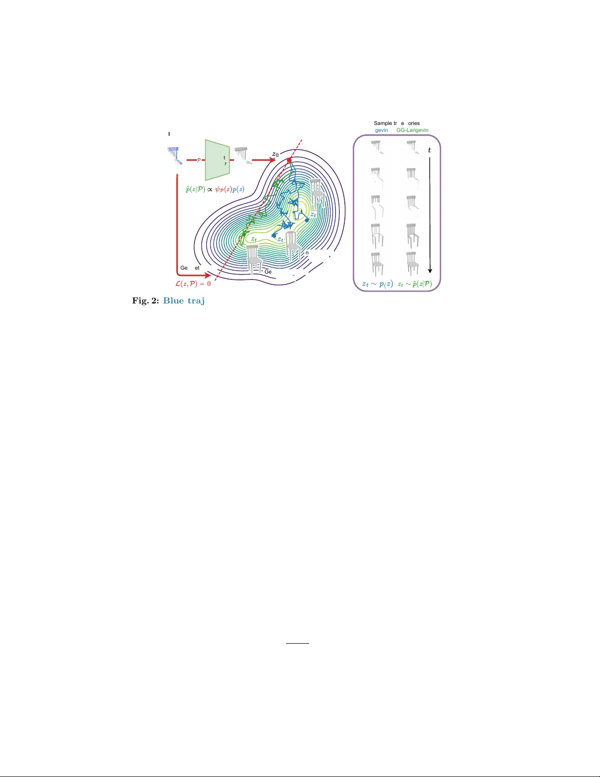
Generativ e Shap e Reconstruction with Geometry-Guided Langevin Dynamics Lin us Härenstam-Nielsen 1 , 2 , Dmitrii P ozdeev 1 , Thomas Dagès 1 , 2 , Nikita Araslanov 1 , 2 , and Daniel Cremers 1 , 2 1 T ec hnical Universit y of Munic h 2 Munic h Center for Machine Learning Abstract. Reconstructing complete 3D shap es from incomplete or noisy observ ations is a fundamen tally ill-p osed problem that requires balancing measuremen t consistency with shape plausibility . Existing metho ds for shap e reconstruction can ac hieve strong geometric fidelity in ideal con- ditions but fail under realistic conditions with incomplete measuremen ts or noise. At the same time, recen t generative mo dels for 3D shap es can syn thesize highly realistic and detailed shapes but fail to be consisten t with observed measurements. In this work, we introduce GG-Langevin: Geometry-Guided Langevin dynamics, a probabilistic approach that uni- fies these complementary p erspectives. By trav ersing the tra jectories of Langevin dynamics induced by a diffusion mo del, while preserving mea- suremen t consistency at ev ery step, we generativ ely reconstruct shap es that fit b oth the measuremen ts and the data-informed prior. W e demon- strate through extensive experiments that GG-Langevin ac hiev es higher geometric accuracy and greater robustness to missing data than existing metho ds for surface reconstruction. Keyw ords: 3D shape reconstruction · Diffusion · Langevin dynamics 1 In tro duction Reconstructing complete shap es from incomplete point clouds is a central chal- lenge in 3D reconstruction with applications in rob otics, 3D scanning, and aug- men ted reality . Sensors, such as LiDAR and depth cameras, pro duce noisy , sparse, and incomplete p oin t clouds, and the task is to recov er a full surface that explains these observ ations. The problem is inherently am biguous: noise must b e disambiguated from structure, and there are often multiple plausible shap es that explain the same input. Solving this problem requires sim ultaneously en- forcing measuremen t consistency (agreement with the observed geometry) and prior consistency (agreemen t with the manifold of realistic shap es). T w o dominan t paradigms tackle these asp ects indep enden tly . Optimization- based methods, suc h as IGR [ 18 ] and DiffCD [ 20 ], fit an implicit surface to Pro ject av ailable at https://github.com/linusnie/gg- langevin . 2 Härenstam-Nielsen et al . Measurement consistency GG-Langevin Measurement and prior consistent Prior consistency Measurements Sparse, noisy , incomplete point cloud 3D shape prior Learned by diffusion model Fig. 1: GG-Langevin. W e combine the prior learned by a diffusion model with gra- dien ts from a geometric loss at inference time. By guiding the tra jectories of Langevin dynamics, we obtain shap es that are b oth measurement-consisten t and prior-consistent. the data b y minimizing a geometric loss function. Optimization-based meth- o ds excel at enforcing measurement consistency but lack data-informed priors, leading to ov ersmo othed or implausible results when observ ations are missing or unreliable. In contrast, learning-based approac hes, suc h as NKSR [ 21 ] and Shap eF ormer [ 48 ], learn to infer shap es directly from p oint clouds by training on large datasets of syn thetically generated p oin t cloud scans. Y et in practice, these mo dels often fail to sim ultaneously preserve b oth measurement consistency and prior consistency , esp ecially when the noise mo del at inference time differs from the noise mo del used during training. Separately from reconstruction, 3D generative mo dels hav e adv anced signif- ican tly in recent y ears, particularly diffusion and flo w mo dels. These models pro vide highly accurate estimates of the prior distribution of 3D shap es when trained at sufficient scale, synthesizing detailed and realistic shap es. How ever, while accurately capturing the prior, effectiv ely leveraging generativ e mo dels for 3D reconstruction remains an op en problem. Our work closes this critical gap. In this work, we combine the b enefits of optimization-based metho ds with the sample quality of generativ e mo dels by lev eraging a generative mo del as a prior. By doing so, we sim ultaneously achiev e b oth high measurement consistency and high prior consistency , as demonstrated in Fig. 1 . Our key insight is to rein terpret the optimization problem probabilistically as sampling shap es from a geometry- guided shape distribution. W e can then replace optimization tra jectories with sto c hastic tra jectories using Langevin dynamics, guided b y the gradients of a geometric loss function. In particular, we construct the geometry-guided shap e distribution b y w eigh ting the prior distribution with a per-sample geometric w eight, such that the sampling tra jectories inheren tly lead to shap es that are b oth measurement-consisten t and prior-consistent. W e refer to our approach as GG-Langevin (Geometry-Guided Langevin dynamics). T o efficiently sample from the geometry-guided distribution, w e develop a no vel Half-Denoising-No-Denoising (HDND) sampling algorithm, which enables Geometry-Guided Langevin Dynamics 3 the diffusion mo del to op erate on noisy latents (half-denoising) while the geomet- ric loss operates on denoised latents (no-denoising). Crucially , the half-denoising comp onen t relies on recen t theory dev elop ed by Hyv ärinen [ 22 ], which we extend with guidance. F urthermore, since our metho d op erates in the latent space of a V AE, it rep eatedly inv ok es the decoder during sampling, which necessitates an inexp ensiv e yet accurate decoder. T o address this, we rebalance the arc hitecture of the widely adopted V ecSet-based V AE [ 52 ] by mo ving the encoder-deco der b ottlenec k, yielding a smaller deco der. Interestingly , our rebalancing improv es not only inference sp eed but also reconstruction qualit y . W e v alidate our approach b y establishing t w o c hallenging surface reconstruc- tion b enc hmarks with sparse and incomplete point clouds. In terms of recon- struction accuracy , GG-Langevin consisten tly outp erforms prior state-of-the-art metho ds by a substan tial margin across all tested ob ject categories. Our core con tributions can b e summarized as follows: – GG-Langevin. W e combine neural implicit surface fitting with the gener- ativ e prior from a pre-trained diffusion mo del, using Langevin dynamics as the theoretical basis. Our generativ e shap e reconstruction method bridges the worlds of optimization and generativ e mo dels, yielding highly accurate 3D shap es from sparse, noisy , and incomplete p oint clouds. – HDND. W e extend the recently developed half-denoising formulation [ 22 ] with denoising-free guidance. Our hybrid Half-Denoising-No-Denoising ap- proac h is particularly suited for the complex guidance functions typically emplo yed for surface reconstruction. – Rebalanced shap e V AE. T o enable efficient inference with GG-Langevin, w e carefully rebalance the reference V ecSet [ 52 ] V AE arc hitecture b y mo ving the b ottlenec k. W e then train our diffusion mo del on the new latent space. 2 Related w ork 2.1 Shap e reconstruction Existing shap e reconstruction approac hes can b e broadly categorized as follo ws: i) optimization-based, where the shap e is estim ated b y minimizing a hand- crafted loss function, ii) learning-based, where it is estimated with a feed-forward mo del trained on correspondences b et ween measurements and full shap es, or iii) optimization-based with a learned prior. Optimization-based. Optimization-based methods work by defining a loss function, whic h can b e minimized iterativ ely [ 1 – 3 , 12 , 20 , 29 , 30 , 37 , 45 ]. V arious w orks propose to regularize optimization-based methods with additional loss terms to stabilize training [ 4 , 37 , 44 , 49 , 58 ], typically biasing the reconstruction to ward smo other surfaces [ 20 , 49 ]. Due to their iterative nature, optimization- based metho ds can achiev e strong consistency with the provided measuremen ts. Ho wev er, due to the lack of a data-informed prior, these metho ds struggle with partial measurements or extreme noise. 4 Härenstam-Nielsen et al . Learning-based. Another line of work estimates shap es directly from p oin t clouds using a learned feed-forw ard mo del to estimate the shape as a v oxel- grid [ 13 , 19 ], point cloud [ 8 , 50 , 57 ], or neural field [ 5 , 17 , 28 , 31 , 32 , 47 , 48 ]. Learning- based metho ds can learn to handle complex measurement noise but t ypically struggle with lo w surface detail, often estimating o verly smo oth shap es [ 20 ]. Learned prior. Some methods combine the tw o approac hes b y separately learning a generic shap e prior, whic h is then used in com bination with an optimization-based metho d at inference time. A core approach in this category is DeepSDF [ 34 ], which learns a latent space that can b e deco ded to SDF v alues using an MLP . With KL-regularization, it is then p ossible to p erform maxim um a p osteriori (MAP) inference o v er shapes. Anothe r approac h is to use Neural Kernel Fields [ 21 , 47 ], whic h learn to extract k ernel parameters from the p oint cloud. These kernel features are then con verted to SDF v alues by solving a kernel regression problem. Our metho d also fits into the learned prior category , using a 3D latent diffusion mo del as the learned prior and GG-Langevin for inference. 2.2 Generativ e mo dels for 3D shap es The adv ent of large open datasets of 3D shap es [ 14 , 15 ] has enabled scalable generativ e modeling in the 3D domain. F ollowing similar trends in the vision domain [ 36 ], generativ e models are t ypically trained in the latent space of an au- to encoder. F or 3D shapes, the predominant auto enco der is 3DShap e2V ecSet [ 52 ] (V ecSet), which repres en ts each shap e as a set of latent vectors that can b e de- co ded into Signed Distance Field (SDF) v alues or o ccupancy . The V ecSet ap- proac h has enabled the training of large diffusion models [ 25 , 27 , 41 , 42 , 55 , 56 ] with v arious conditioning mo dalities, including sketc hes, p oint clouds, and multi- view images. There hav e b een additional improv ements to mak e the underlying auto encoder more expressiv e [ 7 , 53 ] and efficien t [ 9 , 25 , 53 ], increasing its ap- plicabilit y for do wnstream tasks. Shape diffusion mo dels can also b e explicitly trained to sample complete shap es from partial measurements b y conditioning the sampling on incomplete p oin t clouds [ 10 , 52 ]. How ev er, such approaches lac k strong measurement consistency and require task-sp ecific training. Diffusion guidance. Sev eral works use the gradients of a loss function to guide the sampling tra jectories of a diffusion mo del at inference time. This approach w as first used in the image domain as classifier guidance [ 16 ], in which case the loss function is cross-entrop y o ver the classifier logits. Ho wev er, the practical use of classifier guidance is limited b ecause it requires a loss function that is v alid for noisy data. T o circumv en t this issue, DPS [ 11 ] and LGD [ 38 ] prop ose denois- ing the sample with T weedie’s formula at each step of the sampling tra jectory and computing the loss gradien t on the denoised sample. DAPS [ 54 ] impro ves on the quality of guided samples using annealed Langevin sampling. DPS has b een applied to p oint cloud recons truction [ 33 ], but, as we demonstrate in our exp erimen ts, it do es not extend well to laten t shape reconstruction. Geometry-Guided Langevin Dynamics 5 V ecSe t Encode r n on-guided sample Initialization P Input Point cloud 𝑧 0 Geometry-Guided sample 𝑧 𝑡 𝑧 𝑡 Geometric loss L ( 𝑧 , P ) = 0 ˜ 𝑝 ( 𝑧 | P ) ∝ 𝜓 P ( 𝑧 ) 𝑝 ( 𝑧 ) 𝑡 𝑧 𝑡 𝑧 𝑡 ∼ 𝑝 ( 𝑧 ) 𝑧 𝑡 ∼ ˜ 𝑝 ( 𝑧 | P ) Langevin GG-Langevin Sample trajectories Fig. 2: Blue tra jectories: Non-guided Langevin dynamics on the prior distribution p ( z ) , initialized at an incomplete shape using the V AE enco der z 0 = E ( P ) . It generates plausible, complete shapes but quickly dri fts from the measurements. Green tra jec- tory: GG-Langevin generatively reconstructs the shap e from the input p oin t cloud. By incorp orating gradients from a geometric loss L ( z , P ) , it keeps the sampling tra jectory close to the manifold of measurement-consisten t shap es where L ( z , P ) = 0 (indicated b y the dashed red line). On the right: A side-b y-side comparison of sampling tra jec- tories from Langevin dynamics and Geometry-Guided Langevin dynamics. 3 Generativ e shap e reconstruction with GG-Langevin The task of shap e reconstruction is to estimate a complete shape S from a sparse and noisy point cloud measuremen t P = { x i } N i =1 . In particular, w e consider the case where extreme sparsity and incomplete co verage necessitate a data- informed prior to recov er the full shap e. W e assume access to a diffusion mo del for sampling from the generic data distribution p ( z ) , but that the measurement p osterior p ( z |P ) is unkno wn. That is, the diffusion model does not take the measuremen ts P into accoun t. W e tac kle this problem, whic h w e refer to as gener ative shap e r e c onstruction , with a probabilistic approach based on Langevin dynamics [ 35 , 39 , 46 ]. Sp ecifically , we use guided Langevin dynamics, which we find to b e an ideal framework for making full use of the diffusion prior p ( z ) while k eeping the flexibility of optimization-based metho ds. W e detail our probabilistic approac h and sampl ing metho d in Secs. 3.1 and 3.2 , and then apply it to the surface reconstruction problem in Sec. 3.3 . 3.1 Geometric guidance A natural wa y to add measurement consistency to the diffusion prior p ( z ) is to define a geometry-guided shap e distribution, which constrains the diffusion prior to shap es that are measurement-consisten t: ˜ p ( z |P ) = 1 Z ( P ) ψ P ( z ) p ( z ) . (1) 6 Härenstam-Nielsen et al . Here, Z ( P ) is a normalization constant and ψ P ( z ) = exp ( − η L ( z , P )) is a per- sample weigh ting factor based on a geometric loss function L ( z , P ) . The hyper- parameter η > 0 determines how quic kly the weigh ting factor decays to zero as the geometric loss increases. Intuitiv ely , shap es sampled from ˜ p ( z |P ) satisfy t wo conditions: they are probable w.r.t. the prior p ( z ) , and they are consistent with the measurements by minimizing L ( z , P ) . The challenge no w is to design an efficient metho d for sampling from ˜ p ( z |P ) . Existing metho ds for sampling from ˜ p ( z |P ) are based on solving a reverse- time sto c hastic differential equation [ 11 , 38 , 55 ], starting with random noise z T ∼ N (0 , 1) and ending at the guided distribution z 0 ∼ ˜ p ( z |P ) . In termedi- ate samples are then distributed according to noise-p erturb ed versions of the guided distribution z t ∼ ˜ p t ( z t |P ) = R p t ( z t | z ) ˜ p ( z |P ) d z . How ever, as the score functions of ˜ p t are unav ailable, significant approximations m ust b e applied to obtain a tractable sampling pro cedure, which ultimately degrades sample qual- it y . F rom an algorithmic persp ectiv e, starting the sampling pro cess from random noise is also highly impractical, as the loss function L ( z , P ) is only defined for noise-free latents z . 3.2 Sampling from ˜ p ( z |P ) with HDND As a more appealing alternative, w e prop ose sampling from ˜ p ( z |P ) using a mo d- ified version of Langevin dynamics, adapted to take into accoun t the noisy-data score function s σ ( z ) , while k eeping the b enefits of guidance. Before describ- ing our metho d, w e first briefly review regular (discretized) Langevin dynam- ics [ 35 , 39 , 46 ]. Provided the true (noise-free) score function s ( z ) = ∇ z log p ( z ) of p ( z ) , and a starting p oin t z 0 with p ( z 0 ) > 0 , samples from p ( z ) can b e obtained b y iterating the follo wing up date rule: ˜ z t = z t + σ n, z t +1 = ˜ z t + σ 2 2 s ( z t ) , (2) where n ∼ N (0 , 1) and σ is the noise level. That is, at every step, the sample is p erturb ed by noise as well as mov ed tow ards the direction of increasing prob- abilit y . If the true score function s ( z ) was av ailable, we could therefore sample from ˜ p ( z |P ) b y simply plugging ˜ p ( z |P ) in to Eq. ( 2 ): ˜ z t = z t + σ n, z t +1 = ˜ z t + σ 2 2 s ( z t ) − β ∇ z L ( z t , P ) , (3) where β = η σ 2 2 is the effective guidance strength. The k ey adv antage of Eq. ( 3 ) for our purp ose is that z t is approximately distributed according to the geometry- guided distribution ˜ p ( z |P ) at ev ery step, pro vided that the initial sample is sufficien tly likely according to the prior distribution. Critically , this ensures that the gradients ∇ z L ( z t , P ) are alwa ys geometrically meaningful without applying an y additional denoising to the in termediate states z t , a fundamental difference from existing metho ds for diffusion guidance [ 11 , 38 , 54 ]. This makes Eq. ( 3 ) an ideal basis for gradien t-based guidance. Ho w ever, we still need to account for the fact that only the noisy-data score functions s σ ( z ) are a v ailable in practice. Geometry-Guided Langevin Dynamics 7 𝑞 ( 𝑧 ; 𝜇 ) ∝ 𝑒 − 𝛽 ( 𝑥 − 𝜇 ) 2 𝑞 ( 𝑧 ; 𝜇 ) ∝ 𝑒 − 𝛽 | 𝑥 − 𝜇 | 𝑝 𝜃 ( 𝑧 ) ˜ 𝑝 𝜃 ( 𝑧 ; P ) ψ ( z | µ ) ∝ e - η ( z - µ ) 2 ψ ( z | µ ) ∝ e - η | z - µ | p ( z ) ˜ p ( z | µ ) Fig. 3: T oy example. Demonstra- tion that our method generates sam- ples from the geometry-guided dis- tribution ˜ p ( z |P ) . Blue: Data distri- bution. Red: T wo v ariants of guid- ance w eight. Green: Geometry-guided pro duct distribution. Solid lines indi- cate the predicted closed-form distri- butions. The histograms show samples generated using regular Langevin dy- namics and GG-Langevin, resp ectiv ely . W e train an MLP diffusion model on samples from a bimo dal Gaussian p ( z ) . The samples closely follow the pre- dicted distributions. W e tak e in to accoun t the noisy-data score function by using a recently devel- op ed half-denoising v ariant of Langevin dynamics [ 22 ]. Namely , it turns out that samples from p ( z ) can b e obtained us- ing the noisy-data score function as well b y simply replacing s ( z t ) with s σ ( ˜ z t ) in Eq. ( 2 ), where σ is a sufficiently small fixed noise lev el. The name “half- denoising” reflects the fact that the result- ing up date rule corresp onds to subtract- ing half of the noise estimated from the noised laten t ˜ z t at ev ery sampling step. Unfortunately , applying half-denoising di- rectly to Eq. ( 3 ) is not practical ei- ther, as it requires computing the score function of the noise-p erturb ed distribu- tion ˜ p t ( z |P ) . So, to arrive at a practi- cal sampling metho d, we prop ose using a h ybrid “Half-Denoising-No-Denoising” (HDND) Langevin up date rule, where w e apply the half-denoising up date rule only to the data term while k eeping the guidance term unc hanged. This w ay , the diffusion mo del alwa ys op erates on noised latents ˜ z t (half-denoising), while the geometric loss alw ays op erates on denoised laten ts z t (no-denoising): ˜ z t = z t + σ n, z t +1 = ˜ z t + σ 2 2 s σ ( ˜ z t ) − β ∇ z L ( z t , P ) . (4) In contrast to Eq. ( 3 ), this up date rule can b e implemented in practice by esti- mating s σ ( z ) with a diffusion model. As L ( z , P ) in our case is a geometric loss, w e refer to Eq. ( 4 ) as Geometry-Guided Langevin dynamics (GG-Langevin). GG-Langevin is effectively the sum of tw o separate Langevin pro cesses: one half-denoised Langevin process on p ( z ) , ensuring consistency with the data dis- tribution, and one regular Langevin pro cess on ψ P ( z ) for geometric guidance, ensuring measuremen t consistency . While this h ybrid approac h only approxi- mately samples from the guided distribution ˜ p ( z |P ) , we find that the approxi- mation holds remark ably w ell in practice. W e demonstrate this with a 1D toy example in Fig. 3 for the loss functions L ( z , µ ) = ( z − µ ) 2 and L ( z , µ ) = | z − µ | with a small MLP diffusion model trained to fit a bimodal Gaussian distribution. Note that the samples generated with GG-Langevin (green histograms) closely matc h the predicted pro duct distribution (solid green lines) in b oth cases. As an inference metho d, GG-Langevin has several key adv antages: it sam- ples from a well-defined distribution, do es not require noise-lev el scheduling b y k eeping σ constan t, and can be efficiently initialized from an initial estimate z 0 ( e.g ., via the p oint cloud enco der, with z 0 = E ( P ) ). In practice, the close resem blance of Eq. ( 4 ) to gradient-based optimization also allo ws us to leverage 8 Härenstam-Nielsen et al . Algorithm 1 Geometry-Guided Langevin dynamics Require: Poin t cloud P , auto enco der ( E , D ), score mo del s σ , guidance strength β , (optionally scheduled) noise σ t . Initialize z 0 = E ( P ) Initialize Adam optimizer O adam with learning rate β for i = 0 , . . . , N − 1 do A dd noise: ˜ z t = z t + σ t n Half-denoising: ˆ z t = ˜ z t + σ 2 t 2 s σ t ( ˜ z t ) Geometric guidance ( 5 , 6 ): g t = ∇ z L ( z t , P ) A dam up date rule z t +1 = O adam ( ˆ z t , g t ) end for return z N Input IGR DiffCD 3DILG V ecSet Shap eF ormer NKSR DeepSDF Ours GT Fig. 4: Reconstruction results on sparse p oin t clouds. Pro vided sparse p oint cloud scans as input, GG-Langevin reco vers the complete surface and fine structures, significan tly improving the reconstruction accuracy in comparison to previous work. mo dern neural netw ork optimizers for efficient conv ergence. With this in mind, w e adapt GG-Langevin for surface reconstruction in the following section. 3.3 Shap e reconstruction T o apply G G-Langevin for surface reconstruction, w e first need to define the shap e parametrization z and the geometric loss function L ( z , P ) for guidance. As shap e parametrization, we use the latent space of a V ecSet v ariational au- to encoder (V AE) [ 52 ], whic h is a commonly used parametrization for large-scale 3D generativ e mo dels [ 25 , 27 , 41 , 42 , 55 , 56 ]. An enco der E is trained to map com- plete p oin t clouds P to latent vectors: z = E ( P ) , and a deco der D is trained to predict the corresp onding SDF v alues D ( z , x ) at query p oin ts x ∈ R 3 . Via the deco der, each latent v ector therefore represents a surface, whic h is obtained b y Geometry-Guided Langevin Dynamics 9 extracting the 0-lev el set S z = { x : D ( z , x ) = 0 } . As the deco der is differen tiable with respect to b oth argumen ts, we can apply well-established loss functions from neural implicit surface reconstruction to optimize for the laten t z that bes t matc hes the input p oin t cloud. In particular, w e use the IGR loss function [ 18 ]: L ( z , P ) = L surface ( z , P ) + λ L eikonal ( z ) , (5) where L surface ( z , P ) = 1 N N X i =1 | D ( z , x i ) | , L eikonal ( z ) = E x ∼ p eikonal  ∥∇ x D ( z , x ) ∥ − 1  2 . (6) Here, L surface ensures that the shap e approximately fits the point cloud p oin ts x i , and L eikonal pushes the SDF to satisfy the eikonal equation ev erywhere in the b ounding volume Ω = [ − 1 , 1] 3 [ 18 ]. Although v arious extensions to Eq. ( 5 ) ha ve b een prop osed [ 4 , 20 , 37 , 44 , 45 , 58 ], we find that the diffusion prior on its o wn provides sufficien t regularization for highly accurate surface reconstruction. W e provide a visual ov erview of our metho d in Fig. 2 . The sampling tra jectory starts at the initial estimate z 0 , which is typically inaccurate and therefore lies in a lo w-probability region. Then, at eac h iteration, the score function term completes the shape by pulling the sample to wards the shap e distribution, while the guidance term maintains measurement consistency , i.e ., L ( z , P ) ≈ 0 . 3.4 Implemen tation details Enco der initialization. Although the enco der E is trained on complete and noise-free p oin t clouds, we find that it often provides a reasonable estimate ev en when the p oin t cloud is noisy and incomplete. It can therefore naturally b e used to initialize our metho d, reducing the total n umber of iterations required to con verge to the complete shap e. That is, we initialize with z 0 = E ( P ) . Guidance strength. The guidance strength β is a tunable parameter, de- termining the relative strength of the geometric prior. W e note that Eq. ( 4 ) resem bles gradient descent on the effectiv e loss function − log p ( z ) + β L ( z , P ) with an added noise term. Consequently , we use the Adam optimizer [ 24 ] to compute gradient up dates. See Algorithm 1 for a summary of our approac h. Efficien t auto enco der design. At each step of GG-Langevin, we need to compute gradients of the deco der D ( z , x ) . This imp oses some new requiremen ts on the deco der design, namely that it sh ould b e differentiable and as efficien t as p ossible. In con trast, the enco der E ( P ) is only used once at initialization. This raises some issues with existing V ecSet auto encoder designs [ 27 , 42 ], as they employ small enco ders consisting of a single cross-atten tion lay er and, cor- resp ondingly , large deco ders. The large deco der naturally makes the gradients ∇ z L ( z , P ) computationally exp ensiv e. W e alleviate these issues b y moving the enco der-decoder b ottlenec k to a later lay er. This leads to a more expressive la- ten t space due to the larger enco der, while also significantly reducing the time required for propagating gradients from the geometric loss to the latent space. 10 Härenstam-Nielsen et al . T able 1: Shap e reconstruction. Comparison of different metho ds on ShapeNet categories for sparse and incomplete scans. Low er is better for both Chamfer Distance × 10 2 (CD) and Chamfer Angle (CA) in degrees. W e highlight the b est-performing metho d in each ob ject category in b old and the second-b est underlined. Sparse Scans Incomplete Scans Cars Airplanes T ables Chairs Cars Airplanes T ables Chairs CD CA CD CA CD CA CD CA CD CA CD CA CD CA CD CA Optimization IGR [ 18 ] 1.07 27.7 2.80 33.4 2.36 25.1 2.52 29.1 4.47 32.8 3.82 31.7 6.04 29.2 5.38 30.4 DiffCD [ 20 ] 1.22 29.3 0.88 25.7 1.48 21.0 1.58 24.1 5.40 33.1 3.26 28.4 6.02 23.5 5.13 26.0 Learning-based 3DILG [ 51 ] 1.68 30.6 1.01 25.9 1.37 23.1 1.38 26.7 5.50 32.4 4.40 24.3 4.80 18.2 4.51 22.8 V ecSet [ 52 ] 1.81 32.5 0.99 26.8 1.29 17.7 1.23 22.6 5.55 36.1 3.36 23.1 5.31 18.9 4.96 23.8 ShapeF ormer [ 48 ] 1.92 32.0 2.18 33.5 2.10 20.2 2.66 28.6 2.37 30.6 2.75 34.0 2.77 20.4 4.11 32.8 Learned prior DeepSDF [ 34 ] 1.26 34.4 1.55 39.5 1.51 25.8 1.65 30.4 3.83 37.9 3.41 42.0 2.69 25.4 2.44 30.9 NKSR [ 21 ] 1.17 28.6 1.26 29.7 1.44 18.6 1.31 21.5 4.57 31.6 3.62 29.1 5.16 21.8 4.32 23.4 Ours 0.88 25.4 0.63 17.7 1.22 14.3 1.04 17.0 0.84 23.3 1.24 17.6 1.61 15.0 1.95 19.2 Second, we train the auto enco der to predict full, untruncated SDF v alues, en- suring that the eik onal constrain t is satisfied ev erywhere in Ω . W e pro vide a high-lev el o verview of the auto encoder arc hitecture in Fig. 8 and ev aluate our p erformance for different b ottlenec k p ositions in Sec. 4.3 . 4 Exp erimen ts Shap e reconstruction b enc hmark. W e ev aluate surface reconstruction un- der t wo settings: sp arse p oint cloud scans with noise and inc omplete p oint cloud scans with large missing regions. In b oth cases, w e generate p oin t cloud scans using a realistic scanning pro cedure similar to Erler et al . [ 17 ]. W e use v arious t yp es of shap es (Cars, Airplanes, T ables, and Chairs) from Shap eNet [ 6 ]. The resulting point clouds exhibit spatially v arying sparsit y and occasionally contain o ccluded regions. T o generate incomplete scans, w e randomly select a plane nor- mal and an offset, and remov e p oin ts on one side of the plane with a probability that exp onen tially deca ys w.r.t. the distance to the plane. This makes the gen- erativ e prior essen tial to complete the shap e. W e demonstrate in Sec. 4.1 that no existing metho d for surface reconstruction consistently p erforms w ell across this challenging b enc hmark, a gap that our metho d closes. Auto encoder training. W e train our rebalanced V AE from scratch with full un truncated SDF outputs on all Shap eNet [ 6 ] classes. The data and training pip eline is based on V ecSet [ 52 ], and w e use the L1 loss on the ground-truth SDF v alues along with an eikonal loss [ 18 ]. Apart from our rebalanced b ottleneck, w e also ev aluate our metho d with tw o other b ottlenec k p ositions in Sec. 4.3 . Diffusion mo del training. T o appro ximate the noisy-data score functions s σ ( z ) of the shape prior p ( z ) , we train a diffusion model on the latent space of the rebalanced V AE. See Sec. A for implemen tation details. W e train our diffusion mo del without class conditioning, so the ob ject category is unknown at inference time. W e inv estigate adding class conditioning in Sec. E . Hyp erparameters. As base settings, we use N = 2000 iterations of GG- Langevin, with σ = 0 . 05 (constant), β = 0 . 03 , and λ = 0 . 1 . W e in vestigate the Geometry-Guided Langevin Dynamics 11 Input IGR DiffCD 3DILG V ecSet Shap eF ormer NKSR DeepSDF Ours GT Fig. 5: Reconstruction results on incomplete p oint clouds. Despite incomplete p oin t cloud scans as input, GG-Langevin reco vers the missing structure with prior- consisten t geometry . By comparison, previous work either struggles to complete the geometry or hallucinates implausible completions. impact of σ and β on reconstruction qualit y in Sec. 4.4 . F or incomplete p oint clouds, we find that the sampling tra jectory can get stuck on incomplete shap es if σ is c hosen to o small. W e therefore anneal the noise level from σ max = 0 . 2 to σ min = 0 . 02 o ver 4000 iterations with a cosine sc hedule, follo wed by 1000 iterations with constan t σ = 0 . 02 ( N = 5000 iterations in total). W e ev aluate the impact of the annealing schedule in Sec. G . W e also inv estigate adding the off-surface loss from Sitzmann et al . [ 37 ] in Sec. C . Baselines. W e compare our metho d against the state-of-the-art metho ds for surface reconstruction. F or optimization-based metho ds, w e compare against IGR [ 18 ], which optimizes L ( z , P ) with an MLP parametrization. W e also ev al- uate DiffCD [ 20 ], whic h extends IGR with a differentiable Chamfer distance to prev ent spurious surfaces. W e use the “medium-noise” settings from DiffCD [ 20 ] for both metho ds, as w e find it provides the b est results. W e also compare against learning-based methods ShapeF ormer [ 48 ], 3DILG [ 51 ], and the V ecSet V AE [ 52 ] (without diffusion), as well as prior-based metho ds DeepSDF [ 34 ] (which we re- train from scratc h as the original weigh ts are not a v ailable) and NKSR [ 21 ]. Sec. 4.1 presen ts the results. W e also in vestigate sampling from ˜ p ( z |P ) with alternate guided sampling metho ds in Sec. 4.2 . 4.1 Results T o measure reconstruction qualit y we compute the Chamfer Distance (CD) and Chamfer Angle (CA) with resp ect to the ground-truth mesh. The Chamfer Angle measures the av erage angle (in degrees) b et w een the normals of the estimated and ground-truth mesh, using the same p oin t corresp ondences as for the Chamfer distance. F or SDF-based metho ds, w e deco de eac h shap e in to a mesh using 12 Härenstam-Nielsen et al . Input MAP DPS DAPS Ours GT Sparse Incomplete Sparse Incomplete Sampler CD CA CD CA MAP 1.00 21.6 3.86 37.5 DPS [ 11 ] 3.26 38.7 4.04 37.8 DAPS [ 54 ] 1.04 23.2 1.55 19.5 Ours 0.95 18.6 1.41 18.8 Fig. 6: Sampler ablation. Performance comparison of metho ds for sampling from the geometry-guided distribution shap e ˜ p ( z |P ) . W e use the same latent space and loss function for all metho ds. The table on the righ t sho ws the Chamfer Distance (CD) and Chamfer Angle (CA) a veraged across all ob ject categories. 0.00 0.05 0.10 0.15 0.20 σ 1 0.6 0.7 0.8 0.9 σ = 0 . 0 5 ( o u r s ) CDx100 ↓ 0.00 0.05 0.10 0.15 0.20 σ 16° 18° 20° 22° 24° 26° 28° 30° σ = 0 . 0 5 ( o u r s ) CA ↓ β=0.05 β=0.03 (ours) β=0.01 Input σ = 0 σ = 0 . 05 σ = 0 . 2 Fig. 7: Impact of noise level σ and guidance strength β on reconstruction p erformance. If σ is to o small relativ e to β the shap e ov erfits the noise. Conv ersely , if σ is to o large, the shap e starts drifting aw ay from the measurements. Marc hing Cub es [ 26 ]. Our main results are sho wn in T ab. 1 . Qualitativ e results are sho wn in Figs. 4 and 5 . F rom T ab. 1 , w e find that our metho d significantly outp erforms all existing metho ds for shap e reconstruction across all categories — often outperforming the second-b est metho d in eac h category b y a substantial margin. F urthermore, while some baselines achiev e comp etitiv e p erformance on one of the b enc hmarks (sparse or incomplete), no single baseline is consistently comp etitiv e across b oth b enc hmarks. F or instance, DiffCD [ 20 ], NKSR [ 21 ], and V ecSet [ 52 ] p erform well on sparse scans but fail on incomplete scans. On the other hand, Shap eF ormer [ 48 ] and DeepSDF [ 34 ] p erform well on incomplete scans, but p o orly on sparse scans relative to the other metho ds. In comparison, our method is uniquely able to make full use of b oth the measurements (for preserving the original shap e) and the prior (for generating missing parts). 4.2 Sampler ablation GG-Langevin is comp osed of tw o comp onen ts: the geometric loss function L ( z , P ) and a method for sampling from the geometry-guided shap e distribution ˜ p ( z |P ) , defined in Eq. ( 1 ). As described in Sec. 3.2 , we develop a no v el sampling metho d, HDND, to sample from ˜ p ( z |P ) . T o v alidate HDND, we also in v estigate sampling from ˜ p ( z |P ) with existing metho ds DPS [ 11 ] and DAPS [ 54 ]. F or a fair com- parison, w e adapt b oth sampling metho ds to use the enco der initialization as describ ed in Sec. F . Since our shap es are parametrized using a V AE, we also Geometry-Guided Langevin Dynamics 13 in vestigate using MAP estimation by minimizing L MAP ( z , P ) = L ( z , P ) + ξ ∥ z ∥ 2 with Adam [ 24 ]. Results for the sampler comparison are shown in Fig. 6 . Our metho d (GG- Langevin with HDND sampling) consistently outp erforms the other sampling metho ds. MAP p erforms surprisingly well in the sparse setting, v alidating the effectiv eness of our V AE design. How ever, in the incomplete setting, MAP com- pletely fails to recov er a plausible shap e in most cases. W e also find that DPS [ 11 ] struggles to pro duce reasonable samples. DPS [ 11 ] estimates a denoised shape at eac h step using the T weedie’s formula, but this estimate turns out to b e highly inaccurate at early steps (where the noise level is high). Computing the geomet- ric loss with these inaccurate estimates results in inv alid guidance, ultimately causing the sampling tra jectory to diverge into blob-like artefacts. D APS [ 54 ] generally outp erforms DPS [ 11 ], yet still pro duces p oor surface quality and spuri- ous geometry . This is b ecause DAPS [ 54 ] uses a decoupled approac h (alternating denoising and guidance as separate steps), which complicates the tradeoff b e- t ween measurement consistency and prior consistency . In contrast to DPS [ 11 ] and D APS [ 54 ], GG-Langevin completely a voids working with high noise levels. It also applies a tigh tly coupled denoising step and guidance at every iteration, making it significan tly easier to main tain the balance b et ween measurement con- sistency and prior consistency . 4.3 Auto encoder ablation W e ev aluate how our V AE b ottleneck p osition affects reconstruction quality by ev aluating alternate V AEs with 25, 10, and 1 deco der lay ers. F or each setting, w e train a V AE on the Chairs category and then a diffu sion model on the corre- sp onding latent space. As sho wn in Fig. 9 , reducing the deco der size from 25 to 10 yields a roughly 2 × speedup p er GG-Langevin iteration. The reduced decoder size also improv es reconstruction results by a significant margin, likely due to the fact that a single enco der lay er cannot learn a sufficiently expressive laten t space for well-behav ed gradien ts ∇ z L ( z , P ) . Reducing the deco der size ev en fur- ther to a single la yer yields another 2 × sp eedup, but again comes at the cost of reduced reconstruction p erformance: a single deco der la yer do es not provide sufficien t structure for gradient-based guidance. Ov erall, our analysis suggests that balancing the num b er of encoder and deco der lay ers pro duces a latent space ideal for b oth generativ e mo deling and gradient-based guidance. 4.4 Hyp erparameter ablation W e in vestigate the impact of the noise level σ and the guidance strength β in Fig. 7 . W e ev aluate p erformance on sparse p oin t clouds from the Airplanes cat- egory with guidance strengths β = 0 . 01 , 0 . 03 and 0.05 for a range of noise levels from σ = 0 to σ = 0 . 2 . F or β = 0 . 03 (which w e use as our base setting), we find that our method generally p erforms w ell for noise levels σ in the range from σ = 0 . 05 to σ = 0 . 1 . The impact of σ is particularly eviden t in the Chamfer An- gle metric: using small v alues of σ results in shap es that ov erfit the p oint cloud, 14 Härenstam-Nielsen et al . 𝑧 𝐸 𝐷 𝐸 𝐷 Ours 𝑧 SDF T -SDF 1 layer V ecSet 25 layers 16 layers 10 layers gradients gradients Fig. 8: Design choices for the auto encoder. W e reduce the size of the decoder while maintaining the ov erall size of the autoenco der. F urther, we predict a full SDF instead of a T runcated SDF (T-SDF) to enable gradients for the geometric prior. 1 Enc. lay er 25 Dec. lay ers 16 Enc. lay ers 10 Dec. lay ers 25 Enc. lay ers 1 Dec. lay er Dec. lay ers CD CA s/it 25 (V ecSet [ 52 ]) 1.28 18.7 0.21 10 (Ours) 1.12 17.0 0.10 1 1.81 24.6 0.06 Fig. 9: Autoenco der ablation. Reconstruction quality with v arying b ottlenec k p o- sition (26 lay ers total). Using 10 deco der lay ers balances quality and inference sp eed. leading to wobbly surfaces with highly inaccurate normals. On the other hand, using large v alues of σ results in shap es that drift aw a y from the measurements and ov erfit the prior. F or the smaller guidance strength β = 0 . 01 , ov erall p erfor- mance degrades due to a narrow er range of optimal noise lev els. F or the higher guidance strength β = 0 . 05 , the guidance steps get to o large, and p erformance b ecomes unreliable (with sp oradic jumps in CD and CA). W e use σ = 0 . 05 for our metho d, which ac hieves a go o d balance b et ween the tw o extremes. 5 Conclusion W e present GG-Langevin, a no vel shap e reconstruction metho d that in tegrates the geometric consistency of optimization-based approaches with the pow er- ful priors of large-scale shap e diffusion mo dels through a simple yet effectiv e Langevin sampling pro cedure. By guiding the sampling tra jectories of a diffu- sion model with the gradients of a geometric loss, GG-Langevin generativ ely reconstructs shap es that are b oth plausible and consistent with observed data, without requiring task-sp ecific retraining or direct conditioning. Extensiv e ex- p erimen ts under challenging conditions demonstrate that our method ac hieves state-of-the-art performance in b oth fidelit y and robustness. Looking forward, our framew ork pushes the b oundaries of generativ e reconstruction — solving complex reconstruction problems b y com bining the strengths of flexible, but generic, generative mo dels with principled measuremen t consistency . Geometry-Guided Langevin Dynamics 15 References 1. A tzmon, M., Lipman, Y.: SAL: Sign agnostic learning of shap es from ra w data. In: CVPR. pp. 2562–2571 (2020) 3 2. A tzmon, M., Lipman, Y.: SALD: Sign agnostic learning with deriv atives. In: ICLR (2021) 3 3. Baorui, M., Zhizhong, H., Y u-Shen, L., Matthias, Z.: Neural-Pull: Learning signed distance functions from p oin t clouds by learning to pull space onto surfaces. In: ICML (2021) 3 4. Ben-Shabat, Y., Koneputugodage, C.H., Gould, S.: DiGS: Divergence guided shape implicit neural represen tation for unoriented p oint clouds. In: CVPR. pp. 19301– 19310 (2022) 3 , 9 5. Boulc h, A., Marlet, R.: POCO: Point conv olution for surface reconstruction. In: CVPR. pp. 6292–6304 (2022) 4 6. Chang, A.X., F unkhouser, T., Guibas, L., Hanrahan, P ., Huang, Q., Li, Z., Sa v arese, S., Savv a, M., Song, S., Su, H., et al.: Shap eNet: An information-rich 3D mo del rep ository . arXiv:1512.03012 [cs.GR] (2015) 10 7. Chen, R., Zhang, J., Liang, Y., Luo, G., Li, W., Liu, J., Li, X., Long, X., F eng, J., T an, P .: Dora: Sampling and b enc hmarking for 3D shap e v ariational auto-enco ders. In: CVPR. pp. 16251–16261 (2025) 4 8. Chen, Z., Long, F., Qiu, Z., Y ao, T., Zhou, W., Luo, J., Mei, T.: AnchorF ormer: P oint cloud completion from discriminative no des. In: CVPR. pp. 13581–13590 (2023) 4 9. Cho, I., Y o o, Y., Jeon, S., Kim, S.J.: Represen ting 3D shap es with 64 latent vectors for 3D diffusion models. In: ICCV (2025) 4 10. Ch u, R., Xie, E., Mo, S., Li, Z., Nießner, M., F u, C.W., Jia, J.: DiffComplete: Diffusion-based generative 3D shap e completion. In: NeurIPS. vol. 36, pp. 75951– 75966 (2023) 4 11. Ch ung, H., Kim, J., Mccann, M.T., Klasky , M.L., Y e, J.C.: Diffusion p osterior sampling for general noisy inv erse problems. In: ICLR (2023) 4 , 6 , 12 , 13 , iv , v 12. Coiffier, G., Béth une, L.: 1-Lipsc hitz neural distance fields. In: Computer Graphics F orum. vol. 43 (2024) 3 13. Dai, A., Ruizhongtai Qi, C., Nießner, M.: Shap e completion using 3D-enco der- predictor CNNs and shape synthesis. In: CVPR. pp. 5868–5877 (2017) 4 14. Deitk e, M., Liu, R., W allingford, M., Ngo, H., Mic hel, O., Kusupati, A., F an, A., Laforte, C., V oleti, V., Gadre, S.Y., et al.: Ob jav erse-XL: A universe of 10M+ 3D ob jects. In: NeurIPS. vol. 36, pp. 35799–35813 (2023) 4 15. Deitk e, M., Sch w enk, D., Salv ador, J., W eihs, L., Michel, O., V anderBilt, E., Sc hmidt, L., Ehsani, K., Kem bhavi, A., F arhadi, A.: Ob jav erse: A univ erse of annotated 3D ob jects. In: CVPR. pp. 13142–13153 (2023) 4 16. Dhariw al, P ., Nichol, A.: Diffusion mo dels beat GANs on image syn thesis. In: NeurIPS. vol. 34, pp. 8780–8794 (2021) 4 17. Erler, P ., Guerrero, P ., Ohrhallinger, S., Mitra, N.J., Wimmer, M.: Poin ts2Surf learning implicit surfaces from p oin t clouds. In: ECCV. pp. 108–124 (2020) 4 , 10 18. Gropp, A., Y ariv, L., Haim, N., Atzmon, M., Lipman, Y.: Implicit geometric reg- ularization for learning shapes. In: ICML (2020) 1 , 9 , 10 , 11 19. Han, X., Li, Z., Huang, H., Kalogerakis, E., Y u, Y.: High-resolution shap e comple- tion using deep neural netw orks for global structure and lo cal geometry inference. In: ICCV. pp. 85–93 (2017) 4 16 Härenstam-Nielsen et al . 20. Härenstam-Nielsen, L., Sang, L., Saroha, A., Araslanov, N., Cremers, D.: DiffCD: A symmetric differentiable c hamfer distance for neural implicit surface fitting. In: ECCV. pp. 432–447 (2024) 1 , 3 , 4 , 9 , 10 , 11 , 12 , ii 21. Huang, J., Go jcic, Z., Atzmon, M., Litany , O., Fidler, S., Williams, F.: Neural k ernel surface reconstruction. In: CVPR. pp. 4369–4379 (2023) 2 , 4 , 10 , 11 , 12 , iii 22. Hyv arinen, A.: A noise-corrected langevin algorithm and sampling b y half- denoising. TMLR (2025) 3 , 7 , vi 23. Karras, T., Aittala, M., Aila, T., Laine, S.: Elucidating the design space of diffusion- based generative mo dels. In: NeurIPS. vol. 35, pp. 26565–26577 (2022) i , vi 24. Kingma, D.P ., Ba, J.: A dam: A method for sto c hastic optimization. In: ICLR (2015) 9 , 13 25. Lai, Z., Zhao, Y., Zhao, Z., Liu, H., W ang, F., Shi, H., Y ang, X., Lin, Q., Huang, J., Liu, Y., et al.: Unleashing Vecset diffusion mo del for fast shap e generation. In: ICCV. pp. 2523–2533 (2025) 4 , 8 26. Lewiner, T., Lopes, H., Vieira, A.W., T av ares, G.: Efficien t implementation of Marc hing Cub es’ cases with top ological guaran tees. Journal of Graphics To ols 8 (2), 1–15 (2003) 12 27. Li, Y., Zou, Z.X., Liu, Z., W ang, D., Liang, Y., Y u, Z., Liu, X., Guo, Y.C., Liang, D., Ouyang, W., et al.: T rip oSG: High-fidelity 3D shape syn thesis using large-scale rectified flow mo dels. arXiv:2502.06608 [cs.CV] (2025) 4 , 8 , 9 , iii 28. Li, Z.C., Sun, W., Govindara jan, S., Xia, S., Rebain, D., Yi, K.M., T agliasacchi, A.: NoKSR: Kernel-free neural surface reconstruction via p oin t cloud serialization. In: 3DV. pp. 567–574 (2025) 4 29. Ling, S., Nimier-David, M., Jacobson, A., Sharp, N.: Sto chastic preconditioning for neural field optimization. SIGGRAPH (2025) 3 30. Lipman, Y.: Phase transitions, distance functions, and implicit neural representa- tions. ICML (2021) 3 31. Mesc heder, L., Oechsle, M., Niemey er, M., Now ozin, S., Geiger, A.: Occupancy net works: Learning 3D reconstruction in function space. In: CVPR. pp. 4460–4470 (2019) 4 32. Mittal, P ., Cheng, Y.C., Singh, M., T ulsiani, S.: AutoSDF: Shap e priors for 3D completion, reconstruction and generation. In: CVPR. pp. 306–315 (2022) 4 33. Möbius, J.L., Hab ec k, M.: Diffusion priors for Bay esian 3D reconstruction from incomplete measurements. arXiv:2412.14897 [cs.LG] (2024) 4 34. P ark, J.J., Florence, P ., Straub, J., New combe, R., Lo vegro ve, S.: DeepSDF: Learn- ing contin uous signed distance functions for shap e representation. In: CVPR. pp. 165–174 (2019) 4 , 10 , 11 , 12 35. Rob erts, G.O., T weedie, R.L.: Exp onen tial conv ergence of Langevin distributions and their discrete appro ximations. Bernoulli 2 (4), 341–363 (1996) 5 , 6 36. Rom bach, R., Blattmann, A., Lorenz, D., Esser, P ., Ommer, B.: High-resolution image syn thesis with latent diffusion mo dels. In: CVPR. pp. 10684–10695 (2022) 4 37. Sitzmann, V., Martel, J.N., Bergman, A.W., Lindell, D.B., W etzstein, G.: Implicit neural represen tations with p eriodic activ ation functions. In: Pro c. NeurIPS (2020) 3 , 9 , 11 , ii 38. Song, J., Zhang, Q., Yin, H., Mardani, M., Liu, M.Y., Kautz, J., Chen, Y., V ah- dat, A.: Loss-guided diffusion mo dels for plug-and-play controllable generation. In: ICML. pp. 32483–32498 (2023) 4 , 6 39. Song, Y., Ermon, S.: Generative mo deling by estimating gradien ts of the data distribution. In: NIPS. v ol. 32 (2019) 5 , 6 Geometry-Guided Langevin Dynamics 17 40. Song, Y., Sohl-Dickstein, J., Kingma, D.P ., Kumar, A., Ermon, S., Poole, B.: Score- based generative mo deling through sto c hastic differential equations. In: ICLR (2021) vi 41. T encen t Hun yuan3D T eam: Hunyuan3D 1.0: A unified framework for text-to-3D and image-to-3D generation. arXiv:2411.02293 [cs.CV] (2024) 4 , 8 42. T encen t Hunyuan3D T eam: Hunyuan3D 2.0: Scaling diffusion mo dels for high res- olution textured 3D assets generation. arXiv:2501.12202 [cs.CV] (2025) 4 , 8 , 9 , iii 43. Vincen t, P .: A connection b et ween score matc hing and denoising auto encoders. Neural computation 23 (7), 1661–1674 (2011) i 44. W ang, R., W ang, Z., Zhang, Y., Chen, S., Xin, S., T u, C., W ang, W.: Aligning gradien t and hessian for neural signed distance function. In: NeurIPS (2023) 3 , 9 45. W ang, Z., W ang, C., Y oshino, T., T ao, S., F u, Z., Li, T.M.: HotSp ot: Signed dis- tance function optimization with an asymptotically sufficient condition. In: CVPR. pp. 1276–1286 (2025) 3 , 9 46. W elling, M., T eh, Y.W.: Bay esian learning via stochastic gradient Langevin dy- namics. In: ICML. pp. 681–688 (2011) 5 , 6 47. Williams, F., Go jcic, Z., Khamis, S., Zorin, D., Bruna, J., Fidler, S., Litany , O.: Neural fields as learnable kernels for 3D reconstruction. In: CVPR. pp. 18500–18510 (2022) 4 48. Y an, X., Lin, L., Mitra, N.J., Lischinski, D., Cohen-Or, D., Huang, H.: Shap e- former: T ransformer-based shape completion via sparse represen tation. In: CVPR. pp. 6239–6249 (2022) 2 , 4 , 10 , 11 , 12 , iii 49. Y ang, H., Sun, Y., Sundaramo orthi, G., Y ezzi, A.: Steik: Stabilizing the optimiza- tion of neural signed distance functions and finer shape representation. NeurIPS 36 , 13993–14004 (2023) 3 50. Y uan, W., Khot, T., Held, D., Mertz, C., Hebert, M.: PCN: P oint completion net work. In: 3D V. pp. 728–737 (2018) 4 51. Zhang, B., Nießner, M., W onk a, P .: 3DILG: Irregular latent grids for 3D generative mo deling. In: NeurIPS. vol. 35, pp. 21871–21885 (2022) 10 , 11 52. Zhang, B., T ang, J., Niessner, M., W onk a, P .: 3DShape2V ecSet: A 3D shape repre- sen tation for neural fields and generativ e diffusion mo dels. ACM TOG 42 (4), 1–16 (2023) 3 , 4 , 8 , 10 , 11 , 12 , 14 , i 53. Zhang, B., W onk a, P .: LaGeM: A large geometry model for 3D representation learning and diffusion. In: ICLR (2025) 4 54. Zhang, B., Chu, W., Berner, J., Meng, C., Anandkumar, A., Song, Y.: Improving diffusion inv erse problem solving with decoupled noise annealing. In: CVPR. pp. 20895–20905 (2025) 4 , 6 , 12 , 13 , iv , v 55. Zhang, L., W ang, Z., Zhang, Q., Qiu, Q., P ang, A., Jiang, H., Y ang, W., Xu, L., Y u, J.: Clay: A controllable large-scale generative mo del for creating high-quality 3D assets. ACM TOG 43 (4), 1–20 (2024) 4 , 6 , 8 56. Zhao, Z., Liu, W., Chen, X., Zeng, X., W ang, R., Cheng, P ., F u, B., Chen, T., Y u, G., Gao, S.: Michelangelo: Conditional 3D shape generation based on shap e- image-text aligned latent represen tation. NeurIPS 36 , 73969–73982 (2023) 4 , 8 57. Zhou, H., Cao, Y., Chu, W., Zhu, J., Lu, T., T ai, Y., W ang, C.: SeedF ormer: P atch seeds based p oin t cloud completion with upsample transformer. In: ECCV. pp. 416–432 (2022) 4 58. Zixiong, W., Y unxiao, Z., Rui, X., F an, Z., Pengsh uai, W., Shuangmin, C., Shiqing, X., W enping, W., Changhe, T.: Neural-Singular-Hessian: Implicit neural represen- tation of unoriented p oin t clouds by enforcing singular hessian. ACM TOG 42 (6) (2023) 3 , 9 Geometry-Guided Langevin Dynamics i A A dditional implemen tation details In this section, we elab orate on the implementation details for training our re- balanced auto enco der and the corresp onding diffusion mo del. Auto encoder training. W e pre-train our rebalanced V AE ( E , D ) on the Chairs category for 3400 ep ochs, follow ed by 1100 ep ochs on the full dataset, using a batch size of 256 and a learning rate of 5 × 10 − 5 . F or each shap e in each batc h, we sample 1024 p oin ts uniformly from the unit cub e, 1024 points near the surface of the input mesh, and 2048 p oin ts uniformly from the input mesh. The mo del is sup ervised with ground-truth SDF v alues, eikonal loss, and KL- div ergence loss on the b ottleneck la yer. W e follow the pro cedure outlined in [ 52 ] to filter out in v alid p oints on the mesh, suc h as those in the interior of the shap e. W e normalize the input p oin ts to fit inside the unit sphere. In total, autoenco der training takes roughly 3 da ys on 8 A100 GPUs. Diffusion mo del training. F or the diffusion model, w e train a noise predictor ˆ ϵ σ,θ ( z ) , where θ are the mo del parameters and σ is the noise level. W e use the standard noise-prediction ob jective function L diffusion ( θ ) = E z ,σ ,ϵ [ w σ ∥ ˆ ϵ σ,θ ( z + σ ϵ ) − ϵ ∥ 2 ] , (7) where z ∼ p ( z ) , σ ∼ LogNormal( − 1 . 2 , 1 . 2 2 ) (following Zhang et al . [ 52 ]), ϵ ∼ N (0 , I ) , and w σ is a weigh ting factor dep enden t on the noise lev el. W e set w σ = 1 + σ 2 follo wing Karras et al . [ 23 ]. Once the diffusion mo del has b een trained, w e can estimate the noisy-data score function s σ using [ 43 ] s σ ( z ) = − 1 σ ˆ ϵ σ,θ ( z ) . (8) F ollowing Karras et al . [ 23 ], w e parametrize the noise predictor as ˆ ϵ σ,θ ( z ) = 1 √ 1 + σ 2 ϕ σ,θ  z √ 1 + σ 2  + σ 1 + σ 2 z , (9) where ϕ σ,θ is a transformer with 12 lay ers ha ving 8 heads each of dimension 64. The final MLP lay er is selected such that ϕ σ,θ ( z ) = 0 at initialization. Note that the v ariance of the data satisfies σ 2 data = E [ ∥ z ∥ 2 ] ≈ 1 since the auto encoder is trained with KL regularization. A simple calculation then rev eals that the training ob jectiv e satisfies L diffusion ( θ ) ≈ 1 at initialization. W e train the diffusion mo del for 5000 ep o c hs with a batch size of 512 on the Cars, Airplanes, T ables and Chairs categories with a learning rate of 10 − 4 and 10% dropout. F or each shap e in each batch, we obtain latents to denoise b y sampling 1024 p oin ts { x i } 1024 i =1 from the ground-truth mesh in the same w ay as for the auto encoder training and obtain z = E ( { x i } 1024 i =1 ) with the enco der. T raining the diffusion mo del tak es roughly 5 da ys on 8 A100 GPUs. B F ailure cases While GG-Langevin reconstructs the correct shape in most cases, it can get stuc k in suboptimal lo cal minima corresp onding to failed reconstructions. W e ii Härenstam-Nielsen et al . Input DAPS Ours GT Incomplete reconstructions Input DAPS Ours GT Spurious geometry Fig. 10: F ailure cases. While rare, failure cases largely fall into tw o categories: in- complete reconstructions, where part of the shape is missing from the reconstruction, and spurious geometry , where redundant geometry is hallucinated. find that failure cases, exemplified by Fig. 10 , can b e broadly split into tw o cate- gories. The first category is incomplete reconstructions, where the reconstructed shap e correctly fits part of the p oin t cloud while leaving some parts incomplete. Incomplete reconstructions can often b e resolved on a p er-shap e basis b y either increasing the num ber of sampling steps or increasing the noise level σ , albeit at the cost of increased runtime or a higher risk of spurious geometry . The second category of failure cases is spurious geometry . In this case, the estimated shap e t ypically fits the p oin t cloud, but ch unks of geometry are added that are incon- sisten t with the rest of the shap e. Additional loss terms [ 20 , 37 ] can sometimes resolv e the issue of spurious surfaces, although at the cost of a higher risk of incomplete reconstructions. C Siren w eigh t comparison Our metho d is compatible with other loss functions at inference time without retraining. In this section, we inv estigate additional regularization of our method b y incorp orating the Siren loss term developed by Sitzmann et al . [ 37 ], L siren ( z ) = | Ω | α 2 E x ∼ U ( Ω )  e − α | D ( z ,x ) |  , (10) with a w eight factor µ . That is, we add the term µ L siren ( z ) to our geometric loss in Eq. ( 5 ). The Siren loss has b een sho wn to appro ximate the surface area of the reconstructed surface [ 20 ], i.e . L siren ( z ) ≈ | S z | , where | · | denotes the surface area. This means that setting µ > 0 biases the reconstruction to ward shap es with a low er surface area. Consequently , using larger v alues of µ typically results in smoother shapes with less spurious geometry , but they also lead to more incomplete reconstructions. W e show reconstruction results using GG-Langevin with µ ∈ { 0 , 10 − 5 , 10 − 4 , 10 − 3 } in Fig. 11 . Note that µ = 0 is our default setting, which we use for all exp erimen ts in the main manuscript. W e find that increasing µ provides a con- sisten t benefit in the sparse setting (by smo othing out the impact of noise and Geometry-Guided Langevin Dynamics iii Input µ = 0 µ = 10 - 5 µ = 10 - 4 µ = 10 - 3 GT Sparse Incomplete Sampler CD CA CD CA µ = 10 − 3 0.90 18.0 2.63 23.3 µ = 10 − 4 0.97 18.8 1.90 22.3 µ = 10 − 5 0.94 18.4 2.02 23.4 µ = 0 (Ours) 0.95 18.6 1.41 18.8 Fig. 11: Siren w eight comparison. Increasing the Siren loss w eight, µ , typically leads to less spurious geometry (top row), but can also lead to incomplete reconstruc- tions (b ottom row). The table shows metrics a veraged across all shap e categories. reducing spurious geometry), but it also leads to consistent degradation in the p erformance on incomplete shap es (by removing v alid parts of the geometry). Since no setting impro ves b oth b enc hmarks, we set µ = 0 for all other exp eri- men ts, noting that larger v alues of µ can b e b eneficial dep ending on the sp ecific problem scenario. D Limitations and future work As demonstrated in Sec. 4.3 , our method requires a diffusion mo del trained on a sufficiently well-behav ed latent space. Existing large-scale diffusion mo dels [ 27 , 42 ] are t ypically trained with truncated SDF s, using a shallow enco der and a deep deco der. A promising direction for future work is therefore to adapt our metho d to work more efficien tly with a broader range of latent representations. Con versely , another direction would be to further inv estigate ho w to design latent spaces that are well-suited for the type of guidance functions that app ear in surface reconstruction problems. Our metho d also requires more computational time than existing feed-forward metho ds [ 21 , 48 ]. The bulk of our computation time is sp en t on computing the gradients of the geometric loss. Therefore, one highly promising extension would b e to reduce the num ber of deco der ev aluations required to reliably obtain a complete shape. F or instance, this can be ac hieved b y adapting our metho d to tak e multiple denoising steps for eac h guidance step, while still main taining measuremen t consistency . E Class conditioning W e use a diffusion model without class conditioning in all our main exp eriments. This means that our method has to indirectly infer the ob ject category (Car, Airplane, T able, or Chair) at inference time. In order to inv estigate ho w this am biguity impacts reconstruction p erformance, we also train a class-conditioned diffusion mo del ϵ σ,θ ( z , c ) , which takes the ob ject class c as input. W e compare our unconditioned mo del with the class-conditioned mo del in Fig. 12 . In terestingly , we see no clear b enefit in adding class conditioning in the sparse setting. In fact, in this setting, the unconditioned mo del ac hiev es a sligh tly lo w er iv Härenstam-Nielsen et al . Input uncond. class-cond. GT Sparse Incomplete Sparse Incomplete Sampler CD CA CD CA Ours (class-conditioned) 0.98 18.6 1.15 17.6 Ours (unconditioned) 0.95 18.6 1.41 18.8 Fig. 12: Adding class conditioning. Comparing GG-Langevin with and without class conditioning. The class-conditioned mo del has a clear adv an tage in the incomplete setting, where predicting the ob ject category from the p oin t cloud is more difficult. In the sparse setting, b oth mo dels p erform similarly . F or all our main experiments, w e use the unconditioned model, which do es not require the class lab el as input. Input no init with init no init with init GT DPS DAPS Sparse Incomplete Sparse Incomplete Sampler CD CA CD CA DPS (no init) 3.62 41.9 4.25 41.8 DPS (with init) 3.26 38.7 4.04 37.8 DAPS (no init) 4.33 36.3 4.82 35.9 DAPS (with init) 1.04 23.2 1.55 19.5 Fig. 13: Initializing baselines. F or a fair comparison, w e adapt existing metho ds DPS [ 11 ] and DAPS [ 54 ] to make use of the enco der initialization z 0 = E ( P ) . In b oth cases, our suggested initialization improv es performance. Chamfer Distance. The b enefit of class conditioning becomes more apparen t in the incomplete setting. F or incomplete p oin t clouds, our method has to rely more heavily on the prior for reconstructing the full shap e. As exp ected, the more accurate prior leads to a more accurate reconstruction. F Initializing DPS and DAPS Existing metho ds for guided sampling like DPS [ 11 ] and DAPS [ 54 ] start from pure noise, without any information ab out the p oin t cloud. In contrast, a key adv antage of our HDND sampler is that it can b e initialized directly from the V AE enco der with z 0 = E ( P ) . While leveraging the initial estimate for the alternativ e samplers is not as straightforw ard, w e find that b oth DPS [ 11 ] and D APS [ 54 ] can also b enefit from this initial guess. F or DPS [ 11 ], we solve the rev erse SDE starting at z 0 = E ( P ) and ending at z ( T ) 0 ∼ N (0 , σ T ) , where σ T = 80 . W e then run the DPS [ 11 ] algorithm using z ( T ) 0 as the initial noise v ector. Geometry-Guided Langevin Dynamics v Input const 2k const 5k cos 2k cos 5k (Ours) GT σ schedule CD CA const 2k 1.89 22.5 const 5k 1.91 23.3 cos 2k 1.72 22.4 cos 5k (Ours) 1.41 18.8 Fig. 14: Noise sc hedule for incomplete scans. Using cosine annealing for the noise lev el σ (rather than constant) and increasing the num ber of steps from 2000 (2k) to 5000 (5k) is beneficial for incomplete p oint cloud scans. F or DAPS, w e initialize from E ( P ) + σ max n , where σ max = 1 and n ∼ N (0 , 1) . Sampling is th en p erformed b y annealing the noise level from σ max to 0 with 250 MCMC steps p er noise lev el. F or both methods, w e use the same total n um b er of sampling steps as for GG-Langevin, resulting in the same num b er of calls to the diffusion mo del and the V AE deco der. W e show that the enco der initialization impro ves the p erformance of b oth DPS [ 11 ] and DAPS [ 54 ] in Fig. 13 . G Noise sc hedule W e find that the noise lev el parameter σ in Eq. ( 5 ) acts as a step size for the learned prior, analogous to ho w the guidance strength β acts as a step size for the geometric guidance. In this case, a single “step” corresp onds to adding noise to the current latent z t (obtaining ˜ z t ), follow ed b y half-denoising with σ 2 2 s σ ( ˜ z t ) . This naturally suggests applying a noise-lev el sc hedule by replacing σ with a time-v arying σ t to dynamically v ary the trade-off b etw een fitting the prior or fitting the measuremen ts during sampling. W e find that sc heduling the noise lev el is particularly important for incom- plete scans. In the incomplete setting, w e need to initially rely more on the prior than on the measurements to allo w the model to first complete the missing parts b efore fo cusing on details. Thus, we find it b eneficial to start the sampling in the incomplete setting with larger prior-based “steps”, i.e . large σ 0 = σ max , and then progressively reduce the reliance on the prior throughout sampling, as the partial shap e b ecomes increasingly complete, by decreasing σ t un til σ N = σ min . Sp ecifically , we use a cosine-annealing schedule for the first 4000 iterations, σ t = σ min + ( σ max − σ min ) cos  π t 4000  , (11) with σ max = 0 . 2 and σ min = 0 . 02 , follow ed by σ t = σ min for another 1000 iterations ( N = 5000 iterations in total). W e v alidate these design c hoices with an exp erimen t in Fig. 14 . The default setting with constant σ = 0 . 05 for N = 2000 iterations (const 2k) achiev es relatively p o or p erformance, since the shap e remains incomplete at the end of sampling. W e find it optimal to combine cosine sc heduling while increasing the num b er of steps to N = 5000 (cos 5k). vi Härenstam-Nielsen et al . Note that the σ -schedule in GG-Langevin is distinct from the noise lev el sc hedules typically used for reverse SDE sampling [ 23 , 40 ]. Notably , we do not require a large initial noise level σ 0 ≫ 1 , that the noise level m ust tend tow ard zero, σ N ≈ 0 , or that σ t is a decreasing function. Our only assumptions about σ t are that it is sufficiently small suc h that the half-denoising approximation applies [ 22 ], and that it is constan t tow ards the end of sampling, such that Langevin dynamics con verges to a stable distribution. Our final stage with 1k steps at a constant noise level σ = 0 . 02 satisfy b oth of these criteria.