cc-Shapley: Measuring Multivariate Feature Importance Needs Causal Context
Explainable artificial intelligence promises to yield insights into relevant features, thereby enabling humans to examine and scrutinize machine learning models or even facilitating scientific discovery. Considering the widespread technique of Shaple…
Authors: Jörg Martin, Stefan Haufe
cc-Shapley: Measuring Multiv ariate F eature Imp ortance Needs Causal Con text J¨ org Martin ∗ 1 and Stefan Haufe 1,2,3 1 Ph ysik alisc h-T ec hnische Bundesanstalt, Berlin, Germany 2 T ec hnisc he Universit¨ at Berlin, Berlin, German y 3 Charit ´ e – Universit¨ atsmedizin Berlin, Berlin, Germany F ebruary 25, 2026 Abstract Explainable artificial in telligence promises to yield in- sigh ts into relev an t features, thereby enabling humans to examine and scrutinize machine learning mo dels or ev en facilitating scien tific disco v ery . Considering the widespread technique of Shapley v alues, we find that purely data-driv en op erationalization of m ultiv ariate feature imp ortance is unsuitable for such purp oses. Ev en for simple problems with tw o features, spurious asso ciations due to collider bias and suppression arise from considering one feature only in the observ ational con text of the other, which can lead to misinterpre- tations. Causal kno wledge ab out the data-generating pro cess is required to identify and correct suc h mis- leading feature attributions. W e prop ose cc-Shapley (causal context Shapley), an interv en tional mo difica- tion of con ven tional observ ational Shapley v alues lev er- aging kno wledge of the data’s causal structure, thereb y analyzing the relev ance of a feature in the causal con- text of the remaining features. W e show theoretically that this eradicates spurious asso ciation induced by collider bias. W e compare the behavior of Shapley and cc-Shapley v alues on v arious, syn thetic, and real-w orld datasets. W e observ e nullification or rev ersal of as- so ciations compared to univ ariate feature imp ortance when moving from observ ational to cc-Shapley . 1 In tro duction F eature attribution is a common paradigm in the field of Explainable Artificial In telligence (XAI). Its goal is to quantify the importance of each feature b y attribut- ing a score to it. It is often assumed that using such tec hniques allows us to chec k whether a certain mo del is “correct”, i.e., whether it misbehav es on certain data p oin ts or whether it uses unexpected, p ossibly unfa vor- able, structures for its prediction [Rib eiro et al., 2016, Lapusc hkin et al., 2019, Anders et al., 2022]. Lik ewise, ∗ Corresponding author: jo erg.martin@ptb.de XAI is hoped to b o ost scientific discov ery b y unv eil- ing hidden multiv ariate patterns in the data that are asso ciated with prediction targets of in terest [Jim ´ enez- Luna et al., 2020, W ong et al., 2024, Samek and M ¨ uller, 2019]. All of these promises are based on the assump- tion that the attributions gained with such metho ds do not show spurious patterns and can b e in terpreted unam biguously . This w ork aims to show that this as- sumption is an illusion unless we include causal kno wl- edge into our considerations. Our analysis fo cuses on Shapley v alues, a concept of game-theoretical origin that has b ecome a well- established approac h to XAI. When predicting a target v ariable Y from features F = { X 1 , . . . , X n } the Shap- ley value of a feature X j is defined as 1 [Shapley et al., 1953] ϕ ( X j ) = X S ⊆F \{ X j } |S | !( |F | − |S | − 1)! |F | ! I S ( X j ) , (1) where we introduce the notation I S ( X j ) = E [ Y | X j , S ] − E [ Y |S ] (2) for the change in prediction when we add observ ation X j to the observed features S ⊆ F . F ormula (1) com- putes the weigh ted sum of these changes, where the com binatorial weigh ts can b e interpreted through the probabilit y of randomly drawing S , cf. App endix A. F or binary Y ∈ { 0 , 1 } , as considered b elo w, (2) simpli- fies to a difference of probabilities. The computational complexity b ehind (1) quickly in- creases with |F | . F or this reason, several scalable mo d- ifications hav e b een prop osed, e.g., by Lundb erg and Lee [2017] and Janzing et al. [2020]. W e sho w, ho w- ev er, that even without an y appro ximations put on top, ϕ is unsuitable for the purp oses generally targeted b y XAI. T o illustrate this, we will use the follo wing easy running example throughout this work. 1 There are v arious v ersions of (1), cf. App endix A. 1 Example 1.1 (Breakfast and diabetes) . Supp ose blo o d gluc ose G is me asur e d in a p atient to assess whether he or she has diab etes ( Y = 1 ) or not ( Y = 0 ). Unfor- tunately, the p atient ignor es the do ctor’s r e quest not to e at br e akfast b efor e the test. We assume that the me a- sur e d value G fol lows the (simplifie d) r elation G = 85 + 0 . 4 · C + 40 · Y + U , (3) wher e C denotes the c arb ohydr ate intake during br e ak- fast and U denotes indep endent noise. We assume that Y ∼ Bernoulli(0 . 15) , C ∼ N (60; 25) and U ∼ N (0; 10) . The graph in Figure 1a illustrates the causal struc- ture of Example 1.1: the v alue of G is caused by the v ariables Y and C . The plot on the left of Figure 1b sho ws the Shapley v alues (1) for data generated from this simple problem. A red color indicates a high v alue of a feature, whereas a blue color indicates a low v alue. A p ositiv e Shapley v alue ϕ ( G ) = 1 2 I ∅ ( G ) + 1 2 I C ( G ) in- dicates a p ositiv e asso ciation whereas larger G tend to co-o ccur with larger Y if G is either considered alone ( S = ∅ ) or in the con text of a fixed C ( S = { C } ). As red p oin ts in Figure 1b are concen trated on the right for G , we could conclude that high G v alues makes di- ab etes more likely , whic h matches intuition. W e call this p ositive r elevanc e in the following. The Shapley v alues for C , on the other hand, in- dicate a ne gative r elevanc e : high v alues of C are as- so ciated with a lo wer diab etes probability . Does this imply that a single high carb oh ydrate in take makes it less likely that the patient has diab etes? This seems absurd and righ tly so. The underlying reason is instead something which one might dub the “explain aw ay ef- fect” but whic h is t ypically known as suppr ession in the literature [Conger, 1974]: When the patient consumed man y carb oh ydrates there is no need for diab etes to explain high v alues of G . The presence of suppression in our example can b e read off the causal graph in Fig- ure 1a: the suppressor C is connected to the target Y via a no de G with tw o incoming arrows (known as a c ol lider ). Conditioning on a collider leads to a spuri- ous asso ciation, known as c ol lider bias , which mak es C a suppressor of G . Collider bias and suppression are in this work considered as t wo sides of the same coin, cf. Section 2.2. Not every feature attributed negative rele- v ance b y ϕ will automatically be a suppressor. In other examples a feature can, of course, b e of negativ e rele- v ance as it really causes the target to decrease. Appar- en tly , the “right” in terpretation of a chart like the left one in Figure 1b can v ary from situation to situation. This ambigui ty can easily lead to wrong conclusions and undermines the usability of XAI for purp oses suc h as mo del analysis, let alone for scien tific discov ery . Wh y were we able to tell that a suppression ef- fect rather than a p otential health benefit of one carb oh ydrate-ric h breakfast is a more likely interpre- tation for the negative relev ance of C in Figure 1b? W e had to use something that a purely data-driven G C Y (a) Causal graph for Example 1.1 (b) Shapley (left) and cc-Shapley v alues (right) for Ex. 1.1 Figure 1: Causal graph for Example 1.1 (top), together with the according results for con v entional Shapley v al- ues (1) (b ottom - left) and the cc-Shapley v alues (6) (b ottom - right). Exp erimen tal details are in Appendix C.1. mo del does not hav e: an understanding of the real w orld, enco ded in the causal diagram in Figure 1a. In this article we prop ose to use this understanding for our treatment of the con text v ariables S in (1) via tec hniques from c ausal infer enc e [Pearl, 2009]. This causal mo dification of (1) is called c c-Shapley v alues, and is introduced in Definition 3.1. F or Example 1.1, w e depict the cc-Shapley v alues on the righ t side of Figure 1b. W e observe that the cc-Shapley v alues do not attribute C any imp ortance for diab etes risk, whic h matc hes the intuition. The main contributions of this article are as follows: • W e highlight a fundamental problem underlying non-causal XAI metho ds such as (1). In causal inference, this problem is known as collider bias or suppression. • W e prop ose cc-Shapley v alues, whic h mo dify (1) to use causal information. This is, to the b est of our kno wledge, the first approach designed to a void collider bias without the need to restrict oneself to univ ariate feature imp ortance. • W e present theoretical and experimental results regarding the computabilit y and b eha vior of cc- Shapley v alues in the presence of collider bias. W e use several synthetic and one real world example. Comparison with the literature. There are a plethora of XAI metho ds in the literature, cf. for ex- ample the reviews by Angelov et al. [2021], Minh et al. [2022] and Mersha et al. [2024]. While this w ork fo- cuses entirely on Shapley v alues, the criticism raised here go es b ey ond this sp ecific metho d. T ypically , non- causal metho ds use only observ ational ingredien ts: the data and/or the mo del (which is also trained from the data). As causal information is not recov erable from observ ations alone in general and as collider bias is a causal phenomenon, it is implausible that any com bina- tion of purely observ ational information can eradicate the influence of collider bias. Indeed, Wilming et al. 2 [2023] demonstrate the susceptibility of many p opular XAI metho ds to suppression. There is a growing aw areness that the curren t approac h to XAI needs scrutiny or even revision [F reiesleb en and K¨ onig, 2023, Haufe et al., 2024, Wilm- ing et al., 2022] with some works discussing the need and p ossibilit y for combining XAI with causal con- cepts, e.g., [Carloni et al., 2025, Beck ers, 2022, Karimi, 2025, Holzinger et al., 2019, Sch¨ olk opf, 2022]. V arious w orks prop ose using the underlying causal structure to pro duce counterfactual explanations, see, e.g., the w orks by Karimi et al. [2021, 2020], K¨ onig et al. [2023]. The fo cus in these works is mostly to pro duce coun ter- factuals that are coherent with the actual w orld, but the topic of suppression is not discussed in this con text. Janzing et al. [2020], ? ], ? and ? also discuss Shap- ley v alues and the concept of interv ention. Their ap- proac hes are, how ev er, not usable for cases such as Ex- ample 1.1 as their metho ds either still attribute rele- v ance to the suppressor or no relev ance to any feature in Example 1.1 (cf. Section 3.1). Wilming et al. [2023] study Shapley v alues for a simple suppressor problem for whic h no relev ance is attributed to a suppressor; this statemen t is ho w ever only true for their considered example and a sp ecific approximation to Eq. (1). Haufe et al. [2014] and Clark et al. [2025] discuss the problem of suppression and observ e that a univ ariate approach to feature imp ortance av oids these problems. W e will discuss the relation of our work to this idea in Section 2.2 including a discussion why univ ariate imp ortance is in general not sufficient to assess the relev ance of a feature. 2 Bac kground 2.1 Basics of Causal Inference W e here recall core concepts of causal inference needed in this article and refer to P earl [2009]. In causal infer- ence, the data genererating pro cess b ehind a set of v ari- ables is describ ed by a structur al c ausal mo del (SCM) , whic h is a triplet M = ( V , ( f X ) X ∈V , ( U X ) X ∈V ), where • V is the set of v ariables, • ( U X ) X ∈V is a set of indep endent 2 random v ari- ables, representing noise, and • each v ariable X ∈ V is related to its p ar ents pa X ⊆ V \{ X } and its noise v ariable U X via an assignment function X = f X (pa X , U X ). T o av oid inconsistencies, the relations are assumed to b e acyclic: That is, when drawing arrows from pa X to X for each X ∈ V , we arrive at a directed acyclic graph G = ( V , E ) with edges E . Giv en an instance of the noise v ariables ( U X ) X ∈V , we can find the v alues of 2 Throughout this w ork, we assume that the SCM satisfies the local Marko v assumption, i.e., there are no hidden confounders outside the set V . all X ∈ V through ev aluation of the assignmen t func- tions, starting from the source no des without paren ts. The graph G is called the c ausal gr aph and represents the causal functional dependencies underlying the data generating pro cess. Figure 1a depicts the causal graph for Example 1.1. Statistical asso ciation b et ween v ariables can b e as- sessed by studying the paths in G . A p ath b et ween t wo v ariables is a concatenation of adjacen t edges from E (indep enden t of the direction of the edges) leading from one v ariable to the other. If all edges in a path ha ve the same direction, we denote it by 99K or L99 and call it a c ausal p ath . If a causal path consists of only one edge we call it dir e ct , otherwise indir e ct . A path b et w een t wo sets S and S ′ is called a b ackdo or p ath if it leav es S with an incoming edge. A path is called blo cke d , conditional on a (p ossibly empt y) set Z ⊆ V , if it • contains a Z ∈ Z that acts on this path as a chain → Z → ( or ← Z ← ) or as a fork ← Z → , or • if it con tains a c ol lider → C ← which is neither con tained in Z nor in the anc estors an( Z ) of Z (the set of no des that hav e a causal path leading to Z ). A path is called unblo cke d if it is not blo c ked. If all paths b etw een tw o sets of v ariables S , S ′ ⊆ V are blo c k ed conditional on Z , we call them d-sep ar ate d and write S ⊥ ⊥ G S ′ |Z . d-separation im plies indep endence: S ⊥ ⊥ G S ′ |Z ⇒ S ⊥ ⊥ S ′ |Z . The graph G is called faithful if the reverse direction is alwa ys true. Intervention is the pro cess of creating a new SCM from M by setting a v ariable X ∈ V to a s pecific v alue x , replacing f X (pa X , U X ) b y ˜ f X = x . In terven tion sim ulates the effect of a v ariable when we cut off its usual causes and corresp onds to deleting all incoming arro ws to X in G . W e write do( X = x ) or simply do( X ) for this op eration and M do( X ) for the mo dified SCM. Similarly , w e can define an interv en tion do( X ) on a subset of v ariables X ⊆ V or a sto chastic inter- v ention do( X ∼ q ) when drawing the v alues X from a distribution q instead of using constant v alues. In sup ervised mac hine learning, the t ypical task is to estimate a target v ariable from other v ariables. T o accoun t for this distinction in our setup, we call one v ariable Y ∈ V the tar get and the remaining v ariables F = V \{ Y } fe atur es . The features will b e indexed as F = { X i : 1 ≤ i ≤ n } . 2.2 Collider bias Suppressor V ariables and Collider Bias. In Fig- ure 1b, we observed that ev en for simple problems, un- informativ e features, i.e., features that are independent of the target, can b e attributed importance b y XAI metho ds. This is b ecause these features might b e use- ful to remo ve v ariance from informative features. In the 3 literature, v ariables that are useful in such a secondary sense are known as suppr essor variables , as they can b e used to suppress noise [Horst et al., 1941, Conger, 1974, Darlington, 1968, Kim, 2019]. These references all give different definitions of what a suppressor is, partially contradicting each other or giving definitions that only make sense in a linear framew ork. W e here follo w Wilming et al. [2022] and Haufe et al. [2024] and define suppression through c ol lider bias , the statistical asso ciation that arises due to the unblocking of paths when conditioning on a collider or its ancestors (cf. Section 2.1). W e call a (p ossibly informative) feature a suppr essor if it is connected to the target via paths that contain colliders. In this view, suppression and collider bias are just tw o sides of the same coin: sup- pressors are those v ariables whose asso ciation with the target might b e affecte d by collider bias when condi- tioning on other v ariables. Example 1.1 with the causal graph from Figure 1a is a v ery easy example on ho w the collider G makes C a suppressor. F or general setups and a singleton S = { X k } the middle column of T able 1 summarizes how conditioning on X k can lead to col- lider bias b etw een a feature X j and the target, making X j a suppressor. The ro ws of T able 1 distinguish v ari- ous types of paths b etw een X j and Y . In cells marked in red, conditioning on X k will (p oten tially) lead to collider bias b et w een X j and Y : previously blo c ked paths migh t b ecome unblock ed, inducing statistical as- so ciations along these paths. As the num ber of paths quic kly grows with |F | , the consequences of spurious asso ciation introduced by such effects is likely to b e- come aggrav ated even for low-dimensional problems. Univ ariate imp ortance is insufficien t. The prob- lem of suppressor v ariables and the susceptibility of man y XAI metho ds to them is known in the XAI liter- ature [Wilming et al., 2022, Haufe et al., 2024, K¨ onig et al., 2025, W eic hw ald et al., 2015]. Haufe et al. [2014] observ ed that even the w eights of linear mo dels will highligh t suppression v ariables as relev ant. Clark et al. [2025] and Gjølby e et al. [2025] extended this observ a- tion to generalized additiv e mo dels and lo cally linear explanations. These three works also propose p oten tial remedies for this problem, which could, in a nutshell, b e summarized as (re-)fitting the considered feature X j to the target Y in a univ ariate fashion 3 . In the notation of (2), we can express such an approach as I ∅ ( X j ) = E [ Y | X j ] − E [ Y ] , (4) where w e recall that the conditional exp ectation is the optimal fit of X j on to Y , cf. App endix B.1. The ob- ject (4) is not susceptible to collider bias and thus to suppression as it do es not condition on other features. 3 Haufe et al. [2014] actually propose a metho d that, under the assumption of Gaussianity , is equivalen t to a univ ariate linear regression from target to feature. The regression co efficien t of such a fit equals, up to standard deviations, a linear univ ariate regression from feature to target. P aths τ b et ween X j and Y . . . | X k do( X k ) → X k → exists on τ ✗ or ✓ ⇒ ✗ ✗ or ✓ ⇒ ✗ ← X k → exists on τ ✗ or ✓ ⇒ ✗ ✗ or ✓ ⇒ ✗ → X k ← exists on τ ✗ ⇒ ✗ or ✓ ✗ ⇒ ✗ → C ← exists on τ and X k / ∈ τ , C ∈ an( X k ) ✗ ⇒ ✗ or ✓ ✗ ⇒ ✗ None of the ab ov e no effect no effect T able 1: Change in the state of b eing blo c ked ( ✗ ) or un blo c ked ( ✓ ) for paths b et w een feature X j and tar- get Y when conditioning (middle column) or interv en- ing (right column) on X k . ” ✗ or ✓ ” means that the path is p oten tially unblock ed - dep ending on other path details. Conditioning on X k p oten tially un blo c ks pre- viously blo c ked paths, which can lead to c ol lider bias (cells marked in red). This is av oided by causal inter- v entions do( X k ). In particular, we hav e X j ⊥ ⊥ Y ⇒ I ∅ ( X j ) = 0 so that (4) only highlights features that are statistically asso- ciated with Y , a property called the statistic al asso ci- ation pr op erty (SAP) by Clark et al. [2025], Wilming et al. [2023] and Haufe et al. [2024]. F or Example 1.1, the SAP guarantees that I ∅ ( C ) = 0. Univ ariate imp ortance measures suc h as (4) av oid attributing imp ortance to statistically irrelev an t fea- tures which is necessary to apply XAI for mo del de- bugging and scien tific discov ery . How ever, the in ter- pla y b etw een v ariables is vital to the p erformance of a ML mo del and interactions of v ariables can create information that is not av ailable by lo oking at eac h v ariable on its own as shown b y Example 2.1 (Univ ariate imp ortance is not enough) . L et X 1 , X 2 ∼ Bernoulli( 1 2 ) b e indep endent and Y := X 1 · X 2 . Then I ∅ ( X 1 ) = I ∅ ( X 2 ) = 0 indic ate no im- p ortanc e of the fe atur es wher e as the “higher or der” im- p ortanc e terms I X 2 ( X 1 ) = X 1 X 2 − 1 2 X 2 , I X 1 ( X 2 ) = X 1 X 2 − 1 2 X 1 (c orr e ctly) indic ate imp ortanc e. A more complete XAI metho d will thus ha ve to con- sider the multiv ariate interpla y b et w een v ariables. As w e saw ab ov e, doing this purely based on observ ational data as done b y mainstream approaches can lead to spurious asso ciation that can easily b e misinterpreted. In the following section we demonstrate that using causal information provides a w a y out of this dilemma. 3 Metho dology 3.1 Using the causal context A causal v ersion of Shapley v alues. W e sa w in Section 1 for our running Example 1.1 that, even in 4 this simple case, ob jects such as E [ Y | C , G ] are suscep- tible to the problem of spurious correlations, namely b et w een C and Y conditional on G . W e here prop ose to solve problems of this kind as describ ed in the fol- lo wing. First, abandoning the symmetry betw een the con- sidered features, we prop ose to distinguish in each sce- nario b etw een 1. The v ariable whose imp ortance is to b e studied. 2. The v ariable(s) that describ e the background within which the imp ortance of the v ariable from 1 is studied. W e call these v ariables the c ontext . The “parado xical” behavior for Example 1.1 arose when studying the imp ortance of the feature C (car- b oh ydrate in take) in the con text of a glucose v alue of G . The quantit y E [ Y | C, G ] considers the collider G as an observ ation, which leads to the spurious correlation b et w een the suppressor C and Y . W e here prop ose to apply interventions on the context v ariable(s) instead of conditioning on observed v alues. Definition 3.1. We define the imp ortance of a fea- ture X j in the in terven tional context of features S ⊆ F \{ X j } as I do( S ) ( X j ) = E [ Y | X j , do( S )] − E [ Y | do( S )] . (5) Using (5) we define c ausal c ontext Shapley ( cc- Shapley ) values as ϕ cc ( X j ) = X S ⊆F \{ X j } |S | !( |F | − |S | − 1)! |F | ! I do( S ) ( X j ) . (6) In tervening on the con text allows us to remo ve col- lider bias: F or the case of a univ ariate con text S = { X k } , the rightmost column of T able 1 summarizes the effect of the interv ention do( X k ) on the blo c king of paths b etw een X j and Y . In contrast to a mere conditioning on X k (middle column), the interv en tion do( X k ) do es not unblock previously blo c ked paths. In fact, the same holds for general context v ariables S : Since interv en tion remo ves incoming arrows to S in G , the op eration do( S ) do es not lead to a conditioning on colliders. F or the running Example 1.1, we obtain, from Lem- mas 3.3, 3.4 b elo w and App endix C.1, I do( C ) ( G ) = I C ( G ) ≃ σ ( 2 5 ( G − 0 . 4 C − 109)) − 0 . 15 and I do( G ) ( C ) = I ∅ ( C ) = 0. Note that the information on the suppres- sor C is still used but now counts tow ards the imp or- tance of the informative v ariable G it suppresses. The uninformativ e suppressor feature C is assigned no im- p ortance. This can b e shown to hold in general for an y non-informative feature whenever the underlying causal graph is faithful. Th us, the cc-Shapley v alues as defined in Definition 3.1 fulfill the SAP . Prop osition 3.2 (SAP for Definition 3.1) . Given a fe atur e X j with X j ⊥ ⊥ G Y we have I do( S ) ( X j ) = 0 for any S ⊆ F \{ X j } . This implies that we have X j ⊥ ⊥ G Y ⇒ ϕ cc ( X j ) = 0 for ϕ cc as in (6) . Pr o of. This follows from the fact that an interv en tion on S cannot unblock paths betw een X j and Y , hence X j ⊥ ⊥ G Y | do( S ) and thus X j ⊥ ⊥ Y | do( S ). Wh y not use E [ Y | do( X j , S )] instead? A t first sigh t, it might appear tempting to replace a symmetric ob ject such as E [ Y | X j , S ] with a symmetric interv en- tional analogue suc h as E [ Y | do( X j , S )]. This is the approac h studied by ? and ? and fits into the orig- inal framework prop osed by Shapley et al. [1953], cf. App endix A. How ever, this would delete to o muc h as- so ciation: In an anti-causal setup suc h as the running Example 1.1, where there are no causal paths from the features to wards the target, no feature w ould b e at- tributed imp ortance. 3.2 Estimation Simple cases. Ob jects suc h as E [ Y |S ] and E [ Y | X j , S ] can rather easily b e learned from data via training a mach ine learning mo del of choice that predicts Y from S or { X j } ∪ S , cf. Lemma B.1 in the app endix. In terven tional ob jects such as E [ Y | X j , do( S )] from Definition 3.1 are harder to obtain. But in some cases they match observ ational quan tities as shown by the following t wo lemmas whose pro ofs are in App endix B.2. Lemma 3.3 (Irrelev an t context) . Consider X j ∈ F , S ⊆ F \{ X j } and assume that ther e ar e no c ausal p aths S 99K Y , X j . Then we have E [ Y | X j , do( S )] = E [ Y | X j ] and I do( S ) ( X j ) = I ∅ ( X j ) . F or the running Example 1.1, Lemma 3.3 implies that I do( G ) ( C ) = I ∅ ( C ) = 0 as there are no causal paths G 99K Y or G 99K C and hence G is irrelev ant as context for C . Lemma 3.4 (Interv ention equals observ ation) . Con- sider X j ∈ F , S ⊆ F \{ X j } such that, either • (no bac kdo or paths) ther e ar e no unblo cke d b ack- do or p aths fr om S to X j or fr om S to Y , or • (purely causal setup) ther e ar e no c ausal p aths Y 99K X j , S and no c onfounders H ∈ V \ ( { Y , X j } ∪ S ) with X j L99 H 99K Y or S L99 H 99K Y , then we have the identities E [ Y | X j , do( S )] = E [ Y | X j , S ] and I do( S ) ( X j ) = I S ( X j ) . The feature C in Example 1.1 has no bac kdo or paths so that Lemma 3.4 implies I do( C ) ( G ) = I C ( G ). The same argument implies that for Example 2.1 we hav e I do( X 2 ) ( X 1 ) = I X 2 ( X 1 ) and I do( X 1 ) ( X 2 ) = I X 1 ( X 2 ) and thus ϕ cc ( X 1 ) = ϕ ( X 2 ) = 0 , ϕ cc ( X 2 ) = ϕ ( X 2 ) = 0. Bac kdo or adjustment. In Lemma B.5 in the ap- p endix we provide a form ula for the identification of I do( S ) ( X j ) from observ ational data similar to the back- do or adjustment from P earl [2009]. 5 Algorithm 1: Compute I do( S ) ( X j ) from SCM Input: SCM M , X j ∈ F , context S ⊆ F \{ X j } Output: I do( S ) ( X j ) # Create modified model Create sampler of marginal q ( S ) in M ; Construct M do( S ∼ q ) ; # Fit ML models (NN, XGBoost,...) Sample ( X j , S , Y ) from M do( S ∼ q ) ; E [ Y | do( S )] ← fit S to Y ; E [ Y | X j , do( S )] ← fit X j , S to Y ; # Compute importance I do( S ) ( X j ) ← E [ Y | X j , do( S )] − E [ Y | do( S )] ; return E [ Y | X j , do( S )], I do( S ) ( X j ) Using the SCM. Algorithm 1 summarizes ho w I do( S ) ( X j ) can b e computed given an SCM M . This is the metho d that w e use in Section 4 b elo w. W e first isolate the joint marginal q of the context v ari- ables S within the original mo del M . W e then per- form a sto chastic in terven tion on the SCM to obtain M do( S ∼ q ) . In this mo dified mo del, we can obtain esti- mates of the functions E [ Y | X j , do( S )] and E [ Y | do( S )] via standard m ultiv ariate fitting using data-driven mo dels, cf. Appendix B.4. Unless one is working with synthetic examples, the SCM will naturally not b e kno wn, as we also discuss in Section 3.3 b elow. Ho wev er, giv en a causal graph and a defined noise structure, the functional relations can b e estimated from observ ational data by regressing each feature on its parents [Peters et al., 2017]. W e apply this for the real world example in Section 4 b elo w. 3.3 Limitations Neither the original Shapley v alues (1) nor our causal analogue (6) are scalable in the wa y they are formu- lated here. The num b er of of con text sets S increases swiftly with |F | and for each feature X j and context S t wo data-driven models ha ve to b e fitted to estimate E [ Y | X j , do( S )] and E [ Y | do( S )]. Scalable appro xima- tions [Chen et al., 2023, ? , ? ] could b e a w ay out but w ere not studied in the scop e of this work. The main fo cus of this article is to highlight a systematic weak- ness in the existing approach to XAI and to p oin t out what is necessary to fix it. Another limitation that is shared b y man y other w orks on causality , is the assumption that the causal graph that has generated the data is known. Once w e ha ve obtained this graph, w e can often fit the func- tions ( f X ) X ∈V in the SCM and subsequently apply Al- gorithm 1. This is the procedure that we follow for the real world example in Section 4 b elo w. In sp ecific cases, suc h as linear SCMs with non-Gaussian noise, al- gorithms such as LiNGAM [Shimizu et al., 2011] can b e used, cf. Section 4 b elow, to obtain the causal graph. Figure 2: Comparison of the regression co efficien ts b X 1 | X 2 (left) and b X 1 | do( X 2 ) (righ t) with b X 1 for ran- domly sampled linear SCMs with 9 v ariables. The color enco des the exten t to whic h X 2 acts as collider, cf. Ap- p endix C.2. F or more general approaches to causal discov ery com- pare also the work of Zheng et al. [2018] and the reviews b y Zanga et al. [2022], Glymour et al. [2019]. In the general case, ho wev er, obtaining a v alid causal graph is t ypically non-trivial and often requires exp ert knowl- edge. Moreov er, in accordance with many other works in causal inference, we hav e to assume that the exoge- nous v ariables in our mo del are uncorrelated, whic h is t ypically an ov ersimplification. Finally , the usage of a causal graph assumes that a v ariable has a sp ecific static meaning throughout the dataset, which is t ypically not true for other types of data such as images. Here causal representation learning b ecomes necessary to apply causal techniques [Sc h¨ olkopf et al., 2021, Brehmer et al., 2022, Ahuja et al., 2023]. W e did not use such techniques here and only restrict ourselves to static data. 4 Exp erimen tal results Linear SCMs. W e randomly sample 3,000 linear SCMs with 8 features, i.e., F = { X 1 , . . . , X 8 } , V = F ∪ { Y } , and additive non-Gaussian (Laplacian) noise as describ ed in App endix C.2. F or each SCM, the ef- fect of including univ ariate con text S = { X 2 } on the imp ortance of the v ariable X 1 is studied. Using lin- ear mo dels for the fitting of conditional expectations and for Algorithm 1, we obtain partial regression co- efficien ts b X 1 | X 2 , b X 1 | do( X 2 ) , b X 1 for the X 1 -dep endency of I X 2 ( X 1 ), I do( X 2 ) ( X 1 ) and I ∅ ( X 1 ). Figure 2 compares b X 1 | X 2 vs. b X 1 (left) and b X 1 | do( X 2 ) vs. b X 1 (righ t) for all sampled SCMs. Eac h p oin t represents a different linear SCM. F or the compu- tation of b X 1 | do( X 2 ) w e used the DirectLiNGAM algo- rithm from Shimizu et al. [2011] to identify the causal graph, so that no prior kno wledge ab out the causal structure was used. The color of each p oin t represents ho w man y of the paths betw een X 1 and Y that run through X 2 are blo c ked due to X 2 acting as a collider. This is measured by a heuristic quantit y describ ed in App endix C.2. F or yello w p oin ts, almost all paths b et ween X 1 and 6 Figure 3: Shapley (left) and cc-Shapley (right) v alues for the nonlinear diab etes example considered in Sec- tion 4. Y running through X 2 con tain X 2 as a collider, so that w e exp ect the collider bias to b e most distinct for these p oin ts. W e observe that, in the comparison b X 1 | X 2 vs. b X 1 (left), these p oin ts are usually placed far aw a y from the diagonal, indicating that including the observed v alue of X 2 did c hange the imp ortance of X 1 . F or the in terven tional comparison b X 1 | do( X 2 ) vs. b X 1 (righ t), these p oin ts lie on the diagonal and hence con text X 2 that mostly affects X 1 via collider bias do es not lead to a change in imp ortance attributed to X 1 . Nonlinear case. Consider again the task of predict- ing whether a patient has type 2 diab etes ( Y = 1) or not ( Y = 0). W e assume this time that the patient did ob ey and not eat breakfast, but measure in addition to the blo od glucose G also the av erage blo o d sugar H and the BMI B of the patient. The causal graph for this example is shown in Figure 5a, the (synthetic) SCM is sp ecified in App endix C.3. It is widely accepted that a high BMI B is asso ci- ated with an increased risk of type 2 diab etes [Chan- drasek aran and W eiskirchen, 2024]. When lo oking at the Shapley v alues (1) shown on the left in Figure 3, w e might come to a different conclusion: The BMI B is attributed a negative relev ance for diab etes, which one could easily misinterpret as “high BMI leads to a low diab etes risk”. Using cc-Shapley v alues (6) in- stead leads to the v alues depicted on the righ t in Figure 3. The imp ortance b eha vior of B (and the other fea- tures) now matc hes intuition. This different b eha vior of Shapley and cc-Shapley v alues arises, once more, due to collider bias. The Shapley v alues for B in this example are com- puted as ϕ ( B ) = 1 3 I ∅ ( B ) + 1 6 I G ( B ) + 1 6 I H ( B ) + 1 3 I { G,H } ( B ). As sho wn in the first plot in the top ro w of Figure 4, the context-free quantit y I ∅ ( B ) alone indicates a p ositive relev ance for diab etes risk in line with our exp ectations. The ov erall negative relev ance of large B m ust therefore stem from the terms with con text. The left plot in the middle row of Figure 4 sho ws the v alues of I G ( B ) for v arious choices of B and G as a heatmap. F or G in a certain range, I G ( B ) in- dicates a negativ e relev ance of B . A similar b eha vior can b e observed for H , cf. Appendix C.3. A lo ok at the causal graph in Figure 5a rev eals that H and G act as colliders b et w een B and Y so that conditioning on univariate I ∅ ( B ) I ∅ ( G ) observational I G ( B ) I B ( G ) interventional I do( G ) ( B ) I do( B ) ( G ) Figure 4: V arious terms arising in the computation of the conv entional observ ational Shapley v alues (1) and the cc-Shapley v alues (6) for the (more complex) dia- b etes example introduced in Section 4. The upp er row sho ws (with standard error) the con text-free univ ariate term that coincides for (1) and (6). G , H or { G, H } will create a spurious (here negative) asso ciation with Y leading to the pattern observ ed in Figure 3. Once we use I do( G ) ( B ) instead of I G ( B ), this bias is remov ed and w e observ e no negative relev ance of B in the context of G , as shown b y the first plot in the third row of Figure 4. Interestingly , when we switch the roles of B and G , w e obtain a differen t effect: Lemma 3.4 implies that I do( B ) ( G ) = I B ( G ) as there are no bac kdo or paths to B . Both observ ational and in ter- v entional ob jects no w matc h, cf. the second column of Figure 4, and reveal a p ositiv e relev ance of G . The reason for the context dep endency of I do( B ) ( G ) is that the relation B → G is causal and kno wing B allows us to remo v e the v ariance in G and th us judge the relation b et w een G and Y with more precision. This b eha vior resem bles the observ ations of Section 3: The suppres- sion effect of B on G is now only accounted for in the relev ance of the suppressed v ariable G and do es not affect the imp ortance of the suppressor B . In fact, we ha ve ϕ cc ( B ) = I ∅ ( B ) as w e show in App endix C.3. A real world example. W e consider the dataset from Sac hs et al. [2005], which con tains information on the concentration of v arious proteins. W e use a pre- pro cessed version that discretizes the concentration of 7 B Y H G (a) Diabetes and BMI PKC PKA P38 Jnk Raf Mek Erk Akt (b) Protein data Figure 5: Causal graphs for t wo datasets used in Sec- tion 4. F or the diab etes example (left) the meaning of the v ariables are: bloo d glucose G , a verage sugar H , BMI B and presence of t yp e 2 diab etes Y (target). F or the example from Sachs et al. [2005] (right) the v ari- ables are v arious proteins with known causal graph. The protein PKA is here chosen as target. eac h protein in three categories, which we lab el as 0 , 1 and 2. Details on the dataset and our implementation are contained in App endix C.4. The causal graph, de- picted in Figure 5b, sho ws the causal relation of the 8 considered proteins. W e here consider the task of predicting the amount of the protein PKA . Figure 6a shows the univ ariate imp ortance I ∅ of the three proteins Jnk, PKC and P38 depending on their v alue in the set { 0,1,2 } . The results for all features are con tained in Appendix C.4. As we saw ab o ve in Example 2.1, univ ariate imp ortance is in general not sufficien t to fully explain relev ance. How ev er, we also sa w ab o ve that w e hav e to beware of collider bias when a fundamen tal deviation in the relev ance b eha vior only o ccurs in the observ ational context of other v ariables. Figure 6b sho ws the Shapley v alues (left) and cc- Shapley v alues (right) for the proteins Jnk, PKC and P38 . F or Jnk b oth, Shapley and cc-Shapley v alues, sho w a b eha vior that is comparable to the univ ariate imp ortance sho wn in Figure 6a. F or PKC and P38 the Shapley v alues on the left show a deviation to the univ ariate b ehavior. V arious data p oin ts with a high v alue of P38 are attributed negativ e Shapley v alues. F or PKC we see a mixed or even negative relev ance in con trast to the slight p ositiv e relev ance in Figure 6a. Insp ecting the causal graph in Figure 5b we see that PK C (and hence P38 ) is connected with the target PKA via v arious colliders. Using them as observ ational con text as in (1) therefore b ears the risk of in tro ducing collider bias. Indeed, once we use the context only in a causal manner, we find a relev ance attribution that con trasts less with the univ ariate analysis. In particu- lar the (sligh t) p ositiv e relev ance of PK C is k ept intact b y the cc-Shapley v alues. (a) Univ ariate imp ortance I ∅ (b) Shapley and cc-Shapley v alues Figure 6: Some results of the univ ariate imp ortan t measure I ∅ and the Shapley and cc-Shapley v alues for the data from Sachs et al. [2005]. Only a subset of the proteins shown in the causal graph 5b are depicted here. The results for all proteins are contained in Ap- p endix C.4. 5 Conclusion In this work, w e highlight a blind sp ot in purely obser- v ational approaches to XAI. When studying the rele- v ance of a feature in the observ ational context of the remaining features, collider bias can distort the fea- ture attribution and even flip the p ositive relev ance of a feature to a negativ e one and vice versa. This phe- nomenon can already b e observed for hand-crafted t wo- dimensional problems but also app ears for more com- plex and real world data, and adds to further known bi- ases of XAI metho ds suc h as biases to w ards salient fea- tures [Clark et al., 2026]. An incorrect feature attribu- tion can easily lead to misinterpretations and thereby undermine the typical goals pursued when employing XAI. Eradicating collider bias requires interv ention and is hence b ey ond the reach of the observ ational rung of P earl’s ladder of causation [P earl and Mac kenzie, 2018] on which most XAI metho ds fall. Given causal knowl- edge, w e prop ose cc-Shapley v alues as an approach to correct for spurious asso ciations introduced by collider bias. W e observe in theoretical and exp erimen tal re- sults that incorrect and misleading attribution due to collider bias are indeed remov ed when using cc-Shapley v alues. 8 References Kartik Ahuja, Divyat Maha jan, Yixin W ang, and Y oshua Bengio. Interv en tional causal representation learning. In International c onfer enc e on machine le arning , pages 372–407. PMLR, 2023. Christopher J Anders, Leander W eber, David Neu- mann, W o jciech Samek, Klaus-Rob ert M ¨ uller, and Sebastian Lapuschkin. Finding and removing clever hans: Using explanation metho ds to debug and im- pro ve deep mo dels. Information F usion , 77:261–295, 2022. Plamen P Angelov, Eduardo A Soares, Richard Jiang, Nic holas I Arnold, and Peter M Atkinson. Ex- plainable artificial intelligence: an analytical review. Wiley Inter disciplinary R eviews: Data Mining and Know le dge Disc overy , 11(5):e1424, 2021. Sander Beck ers. Causal explanations and xai. In Con- fer enc e on c ausal le arning and r e asoning , pages 90– 109. PMLR, 2022. bnlearn. Reproducing the causal signalling netw ork in Sac hs et al., Science (2005). https://www. bnlearn.com/research/sachs05/ , 2022. Last ac- cessed: 2026-02-10. Johann Brehmer, Pim De Haan, Phillip Lipp e, and T aco S Cohen. W eakly sup ervised causal represen ta- tion learning. A dvanc es in Neur al Information Pr o- c essing Systems , 35:38319–38331, 2022. Gianluca Carloni, Andrea Berti, and Sara Colantonio. The role of causality in explainable artificial intelli- gence. Wiley Inter disciplinary R eviews: Data Min- ing and Know le dge Disc overy , 15(2):e70015, 2025. Preethi Chandrasek aran and Ralf W eiskirchen. The role of ob esit y in t yp e 2 diab etes mellitus—an o verview. International journal of mole cular sci- enc es , 25(3):1882, 2024. Hugh Chen, Ian C Cov ert, Scott M Lundb erg, and Su- In Lee. Algorithms to estimate shapley v alue feature attributions. Natur e Machine Intel ligenc e , 5(6):590– 601, 2023. Tianqi Chen and Carlos Guestrin. Xgbo ost: A scal- able tree bo osting system. In Pr o c e e dings of the 22nd A CM SIGKDD International Confer enc e on Know l- e dge Disc overy and Data Mining , KDD ’16, page 785–794, New Y ork, NY, USA, 2016. Asso ciation for Computing Mac hinery . ISBN 9781450342322. doi: 10.1145/2939672.2939785. URL https://doi.org/ 10.1145/2939672.2939785 . Benedict Clark, Ric k Wilming, Hjalmar Sch ulz, Rus- tam Zh umagambetov, Dann y Panknin, and Stefan Haufe. Correcting misinterpretations of additiv e mo dels. In The Thirty-ninth Annual Confer enc e on Neur al Information Pr o c essing Systems , 2025. Benedict Clark, Marta Oliveira, Ric k Wilming, and Stefan Haufe. F eature salience – not task- informativ eness – drives machine learning mo del ex- planations. arXiv pr eprint arXiv:2602.09238 , 2026. An thony J Conger. A revised definition for suppressor v ariables: A guide to their identification and inter- pretation. Educ ational and psycholo gic al me asur e- ment , 34(1):35–46, 1974. Ric hard B Darlington. Multiple regression in psycho- logical researc h and practice. Psycholo gic al bul letin , 69(3):161, 1968. An upam Datta, Shay ak Sen, and Y air Zic k. Algorith- mic transparency via quantitativ e input influence: Theory and exp erimen ts with learning systems. In 2016 IEEE symp osium on se curity and privacy (SP) , pages 598–617. IEEE, 2016. Timo F reiesleben and Gunnar K¨ onig. Dear xai com- m unity , w e need to talk! fundamental misconcep- tions in current xai research. In World c onfer enc e on explainable artificial intel ligenc e , pages 48–65. Springer, 2023. Anders Gjølby e, Stefan Haufe, and Lars Kai Hansen. Minimizing false-positive attributions in explana- tions of non-linear mo dels. In The Thirty-ninth An- nual Confer enc e on Neur al Information Pr o c essing Systems , 2025. Clark Glymour, Kun Zhang, and P eter Spirtes. Re- view of causal disco very metho ds based on graphical mo dels. F r ontiers in genetics , 10:524, 2019. Aric Hagb erg, Pieter J Sw art, and Daniel A Sch ult. Exploring net work structure, dynamics, and func- tion using netw orkx. T echnical rep ort, Los Alamos National Lab oratory (LANL), 2007. Stefan Haufe, F rank Meinec ke, Kai G¨ orgen, Sven D¨ ahne, John-Dylan Haynes, Benjamin Blankertz, and F elix Bießmann. On the in terpretation of w eigh t v ectors of linear mo dels in multiv ariate neuroimag- ing. Neur oimage , 87:96–110, 2014. Stefan Haufe, Ric k Wilming, Benedict Clark, Rustam Zh umagambetov, Ahc` ene Boub ekki, J¨ org Martin, and Danny Panknin. Explainable ai needs formal- ization. 2024. arXiv preprint Andreas Holzinger, Georg Langs, Helmut Denk, Kurt Zatlouk al, and Heimo M¨ uller. Causability and explainabilit y of artificial intelligence in medicine. Wiley inter disciplinary r eviews: data mining and know le dge disc overy , 9(4):e1312, 2019. P aul Horst et al. The role of predictor v ariables which are indep enden t of the criterion. So cial Scienc e R e- se ar ch Council , 48(4):431–436, 1941. 9 Dominik Janzing, Lenon Minorics, and Patric k Bl¨ obaum. F eature relev ance quantification in ex- plainable ai: A causal problem. In International Confer enc e on artificial intel ligenc e and statistics , pages 2907–2916. PMLR, 2020. Jos ´ e Jim´ enez-Luna, F rancesca Grisoni, and Gisb ert Sc hneider. Drug disco very with explainable artifi- cial intelligence. Natur e Machine Intel ligenc e , 2(10): 573–584, 2020. Amir-Hossein Karimi. P osition: Explainable ai is causal discov ery in disguise. 2025. Amir-Hossein Karimi, Julius V on K ¨ ugelgen, Bernhard Sc h¨ olkopf, and Isab el V alera. Algorithmic recourse under imperfect causal knowledge: a probabilistic approac h. A dvanc es in neur al information pr o c essing systems , 33:265–277, 2020. Amir-Hossein Karimi, Bernhard Sc h¨ olkopf, and Isab el V alera. Algorithmic recourse: from counterfactual explanations to in terven tions. In Pr o c e e dings of the 2021 A CM c onfer enc e on fairness, ac c ountability, and tr ansp ar ency , pages 353–362, 2021. Y ongnam Kim. The causal structure of suppressor v ari- ables. Journal of Educ ational and Behavior al Statis- tics , 44(4):367–389, 2019. Gunnar K¨ onig, Timo F reiesleben, and Moritz Grosse- W entrup. Impro vemen t-fo cused causal recourse (icr). In Pr o c e e dings of the AAAI Confer enc e on Ar- tificial Intel ligenc e , v olume 37, pages 11847–11855, 2023. Gunnar K¨ onig, Eric G¨ un ther, and Ulrike v on Luxburg. Disen tangling interactions and dep endencies in fea- ture attributions. In Yingzhen Li, Stephan Mandt, Shipra Agraw al, and Emtiy az Khan, editors, Pr o- c e e dings of The 28th International Confer enc e on A rtificial Intel ligenc e and Statistics , v olume 258 of Pr o c e e dings of Machine L e arning R ese ar ch , pages 2134–2142. PMLR, 03–05 May 2025. URL https: //proceedings.mlr.press/v258/konig25a.html . Sebastian Lapuschkin, Stephan W¨ aldc hen, Alexander Binder, Gr ´ egoire Monta v on, W o jciec h Samek, and Klaus-Rob ert M ¨ uller. Unmasking clev er hans predic- tors and assessing what mac hines really learn. Na- tur e c ommunic ations , 10(1):1096, 2019. Stan Lip o vetsky and Michael Conklin. Analysis of re- gression in game theory approach. Applie d sto chas- tic mo dels in business and industry , 17(4):319–330, 2001. M.M. Lo ev e and M.H. Stone. Pr ob ability The- ory: University Series in Higher Mathemat- ics . Literary Licensing, LLC, 2013. ISBN 9781258664541. URL https://books.google.de/ books?id=mUqqmwEACAAJ . Scott M Lundb erg and Su-In Lee. A unified approach to interpreting mo del predictions. A dvanc es in neu- r al information pr o c essing systems , 30, 2017. Melk am u Mersha, Khang Lam, Joseph W oo d, Ali K Alshami, and Jugal Kalita. Explainable artificial in- telligence: A survey of needs, techniques, applica- tions, and future direction. Neur o c omputing , 599: 128111, 2024. Dang Minh, H Xiang W ang, Y F en Li, and T an N Nguy en. Explainable artificial intelligence: a com- prehensiv e review. Artificial Intel ligenc e R eview , 55 (5):3503–3568, 2022. Martin J Osb orne and Ariel Rubinstein. A c ourse in game the ory . MIT press, 1994. Judea Pearl. Causality . Cam bridge universit y press, 2009. Judea P earl. Linear mo dels: A useful “microscop e” for causal analysis. Journal of Causal Infer enc e , 1(1): 155–170, 2013. Judea Pearl and Dana Mac kenzie. The b o ok of why: the new scienc e of c ause and effe ct . Basic b o oks, 2018. Jonas P eters, Dominik Janzing, and Bernhard Sc h¨ olkopf. Elements of c ausal infer enc e: foundations and le arning algorithms . The MIT press, 2017. Marco T ulio Ribeiro, Sameer Singh, and Carlos Guestrin. ” why should i trust you?” explaining the predictions of any classifier. In Pr o c e e dings of the 22nd ACM SIGKDD international c onfer enc e on know le dge disc overy and data mining , pages 1135– 1144, 2016. Karen Sachs, Omar P erez, Dana Pe’er, Dou- glas A. Lauffenburger, and Garry P . Nolan. Causal protein-signaling netw orks derived from m ultiparameter single-cell data. Scienc e , 308 (5721):523–529, 2005. doi: 10.1126/science. 1105809. URL https://www.science.org/doi/ abs/10.1126/science.1105809 . W o jciech Samek and Klaus-Rob ert M ¨ uller. T ow ards explainable artificial intelligence. In Explainable AI: interpr eting, explaining and visualizing de ep le arn- ing , pages 5–22. Springer, 2019. Bernhard Sch¨ olk opf. Causalit y for mac hine learning. In Pr ob abilistic and c ausal infer enc e: The works of Jude a Pe arl , pages 765–804. 2022. Bernhard Sc h¨ olkopf, F rancesco Lo catello, Stefan Bauer, Nan Rosemary Ke, Nal Kalch brenner, Anirudh Goy al, and Y osh ua Bengio. T ow ard causal represen tation learning. Pr o c e e dings of the IEEE , 109(5):612–634, 2021. Llo yd S Shapley et al. A v alue for n-p erson games. 1953. 10 Shohei Shimizu, T ak anori Inazumi, Y asuhiro Sogaw a, Aap o Hyv arinen, Y oshinobu Kaw ahara, T ak ashi W ashio, P atrik O Hoy er, Kenneth Bollen, and Patrik Ho yer. Directlingam: A direct metho d for learning a linear non-gaussian structural equation mo del. Jour- nal of Machine L e arning R ese ar ch-JMLR , 12(Apr): 1225–1248, 2011. Sebastian W eich w ald, Timm Meyer, Ozan ¨ Ozdenizci, Bernhard Sch¨ olk opf, T onio Ball, and Moritz Grosse- W entrup. Causal interpretation rules for enco ding and deco ding mo dels in neuroimaging. Neur oimage , 110:48–59, 2015. Ric k Wilming, C´ eline Budding, Klaus-Rob ert M ¨ uller, and Stefan Haufe. Scrutinizing xai using linear ground-truth data with suppressor v ariables. Ma- chine le arning , 111(5):1903–1923, 2022. Ric k Wilming, Leo Kieslich, Benedict Clark, and Ste- fan Haufe. Theoretical b ehavior of xai metho ds in the presence of suppressor v ariables. In Inter- national Confer enc e on Machine L e arning , pages 37091–37107. PMLR, 2023. F elix W ong, Erica J Zheng, Jacqueline A V aleri, Nina M Donghia, Melis N Anah tar, Satotak a Omori, Alicia Li, Andres Cubillos-Ruiz, Aarti Krishnan, W engong Jin, et al. Discov ery of a structural class of an tibiotics with explainable deep learning. Natur e , 626(7997):177–185, 2024. Sew all W righ t. The metho d of path co efficien ts. The annals of mathematic al statistics , 5(3):161–215, 1934. Alessio Zanga, Elif Ozkirimli, and F abio Stella. A sur- v ey on causal discov ery: theory and practice. In- ternational Journal of Appr oximate R e asoning , 151: 101–129, 2022. Xun Zheng, Bryon Aragam, Pradeep K Ravikumar, and Eric P Xing. Dags with no tears: Contin uous optimization for structure learning. A dvanc es in neu- r al information pr o c essing systems , 31, 2018. 11 cc-Shapley: Measuring Multiv ariate F eature Imp ortance Needs Causal Context (Supplemen tary Material) A On the used v ersion of Shapley v alues Comparison with the li terature. In the con text of game theory , Shapley et al. [1953] introduced a general expression of the form ϕ ( X j ) = X S ⊆F \{ X j } γ ( S )( v ( S ∪ { X j } ) − v ( S )) , (7) where γ ( S ) = |S | !( |F |−|S |− 1)! |F | ! and v : 2 F → R is a general set function that satisfies some simple prop erties and should b e thought of as enco ding a game. Lipov etsky and Conklin [2001] use R 2 for v in the cont ext of linear regression to judge feature imp ortance. Datta et al. [2016] consider a more general framew ork that uses (7) to measure the influence of inputs with v arious choices of v . Referring to the w orks ab o ve, Lundb erg and Lee [2017] formulate a “classic” version of Shapley v alues as ϕ ( X j ) = X S ⊆F \{ X j } γ ( S )( f ( S ∪ { X j } ) − f ( S )) , (8) here f ( S ∪ { X j } ) and f ( S ) denote functions that w ere trained only on the features S ∪ { X j } and S resp ectiv ely . The optimally trained mo dels f ha ve precise mathematical formulations in terms of a conditional exp ectation, cf. Lemma B.1 b elo w. W e can thus iden tify f ( S ∪ { X j } ) = E [ Y |S , X j ] and f ( S ) = E [ Y |S ] and arrive at the expression (1) used in this work. Expression (1) is mo del agnostic in the sense that it only uses optimal mo dels and not a sp ecific instance of a trained mo del. While Lundb erg and Lee [2017] refer to classical Shapley v alues as formulated in (8), their prop osed algorithm SHAP completely builds on the full mo del f ( F ). Janzing et al. [2020] explicitly use the output of the model, called ˆ Y in the follo wing, for their arguments and their algorithm. The approach presen ted in this work is also usable for ˆ Y instead of Y . A simplified, pragmatic adaption might b e to treat ˆ Y as an estimate of Y , which is likely to yield comparable results for mo dels with high accuracy (or low MSE in the case of regression). A more causal approach w ould b e to add a no de ˆ Y to the causal graph and draw arrows from each feature used for training to ˆ Y with the corresp onding assignment function f ˆ Y no w just given by the learned machine learning mo del. Doing so will how ev er not cure the problems inheren t to (1) that we outlined in the main text: Consider again the example with the causal diagram 5a. First, note that Y can actually not simply b e remov ed from the diagram as it acts as a mediator (a chain on a causal path) b et ween B and the no des G and H . Second, there is a collider bias b et ween H and B when conditioning on G so that even with Y completely replaced by ˆ Y w e would hav e terms in (1) that are influenced by collider bias. Summarizing, we b eliev e that the mo del-agnostic approach presented in this work is the most suitable and expressiv e to highlight feature relev ance, as it uses the actual process underlying the data and simplifies matters b y ignoring mo del sp ecific asp ects. On the com binatorial co efficients γ ( S ) . W e mentioned ab ov e that there are v arious versions of Shapley v alues. These versions only differ in their c hoice of v in (1) but keep the same co efficien ts γ ( S ). W e here shortly recall the meaning of γ ( S ) [Osb orne and Rubinstein, 1994] to motiv ate why we also use them in the cc-Shapley v alues from Definition 3.1: If we do not wan t to make an y additional assumptions, it is unclear which features S ⊆ F \{ X j } to use as a con text to judge the relev ance of X j . T o decide this in a fair manner, imagine that w e base our decision on a randomized exp erimen t: W e shuffle the order of features F = { X 1 , . . . , X n } by uniformly drawing from all p erm utations on F . W e then use all v ariables that come b efore X j in such a ordering as context. The probabilit y that the set S ⊆ F is chosen as con text in such an exp erimen t is then just γ ( S ) = |S | !( |F | − |S | − 1)! |F | ! . (9) Here, |S | ! are the n umber of w ays we can reorder S in fron t of X j , ( |F | − |S | − 1)! are the num b er of wa ys we can order the remaining features after X j , and the denominator |F | ! is just the n umber of p erm utations in F . In particular, we see that the co efficien ts in (7) add up to 1. The same logic can b e applied to motiv ate the usage of γ ( S ) for the cc-Shapley v alues in Definition 3.1: W e c ho ose a random subset S ⊆ F \{ X j } as causal context using the same randomized pro cedure. 12 On the asymmetry of cc-Shapley v alues. In Definition 3.1 we introduce the cc-Shapley v alues as ϕ cc ( X j ) = X S ⊆F \{ X j } γ ( S ) ( E [ Y | X j , do( S )] − E [ Y | do( S )]) . (10) W e motiv ated ab ov e the usage of the same co efficients γ ( S ). How ev er, in one other fundamental asp ect this definition differs from (7): The ob jects E [ Y | X j , do( S )] and E [ Y | do( S )] cannot b e understo o d as set functions as they treat X j and S differen tly . Our cc-Shapley v alues therefore lack the symmetry in the treatment of all considered features and, in general, will not ha ve a prop ert y such as P j ϕ ( X j ) = v ( F ) − v ( ∅ ) satisfied b y (7) [Shapley et al., 1953]. F rom a game theoretical viewp oint our asymmetric mo dification means that we give the “pla yer” X j an adv an tage that we don’t grant the other “play ers” S , namely to use non-causal asso ciation. This asymmetric treatment is vital to the p erformance of ϕ cc . In fact, • W e need to allow for non-causal asso ciation b et ween X j and Y to obtain non-trivial imp ortance in anti- causal setups, cf. Section 3. • The con text v ariables S cannot be treated in the same w a y , as we would otherwise allo w X j to be attributed imp ortance that solely arises from suppressing noise in the v ariables S as we observe for Example 1.1. Breaking the symmetric, equal treatmen t of all features in (7) is therefore precisely what allows (10) to correct spurious asso ciations. B F urther theoretical asp ects B.1 Conditional exp ectation as optimal mo del The follo wing basic result recalls that the mathematically optimal mo del for a typical (sup ervised) machine learning problem is given b y the c onditional exp ectation. In particular, this sho ws that w e can obtain an estimate of conditional exp ectations such as E [ Y |S ] with features S ⊆ F simply b y training a data-driv en mo del with input S and target Y using MSE-loss (for regression) or cross-entrop y loss (for classification). Lemma B.1 (Conditional expectation as optimally trained mo del) . Consider a set of squar e-inte gr able r andom variables S and another squar e inte gr able and r e al-value d r andom variable Y define d on the same pr ob ability sp ac e. Then the optimization pr oblem arg min f E [ | Y − f ( S ) | 2 ] (11) has (almost sur ely) a unique solution given by the c onditional exp e ctation E [ Y |S ] . If Y is binary, then E [ Y |S ] = P ( Y = 1 |S ) is mor e over the optimal solution to the pr oblem arg min f E [ L CE ( Y ; f ( S ))] , (12) wher e L CE ( Y ; f ( S )) = − Y log f ( S ) − (1 − Y )(1 − log f ( S )) is the cr oss-entr opy loss. R emark B.2 . A similar statemen t holds for the multiv ariate case or multiclass case (when Y is one-hot-enco ded). Pr o of. The statemen t on L 2-optimalit y (11) is a classical result from probability theory [Lo ev e and Stone, 2013]. The statement based on (12) can b e seen by using the tow er prop ert y of conditional exp ectations: E [ L CE ( Y ; f ( S ))] = E [ E [ L CE ( Y ; f ( S )) |S ]] = − E [ p S log f ( S ) + (1 − p S )(1 − log f ( S ))] , where p S = P ( Y = 1 |S ). Minimizing the inner expression w.r.t f ( S ) (setting the deriv ative to zero), yields f ( S ) = p S = P ( Y = 1 |S ) = E [ Y |S ]. B.2 Pro ofs of Lemmas 3.3 and 3.4 W e here restate the lemmas from Section 3.2 together with their pro ofs. Lemma B.3 (Irrelev an t context) . Consider X j ∈ F , S ⊆ F \{ X j } and assume that ther e ar e no c ausal p aths S 99K Y , X j . Then we have E [ Y | X j , do( S )] = E [ Y | X j ] and I do( S ) ( X j ) = I ∅ ( X j ) . 13 Pr o of. W e apply rule 3 of do calculus [P earl, 2009] to remov e do( S ) from the conditional exp ectation, i.e., we ha ve to verify the following d-separation Y ⊥ ⊥ G S S | X j , (13) where G S denotes the graph where all incoming edges to S were deleted. The actual rule 3 uses G S ( X j ) instead of G S , which denotes the remov al of all ancestors of X j from S . By assumption, S contains, how ever, no ancestors of X j . Consider, conditional on X j , a p oten tial unblock ed path b etw een S and Y in G S . Denote by X k ∈ S the last element within S on the wa y to Y and consider, from now on, the un blo c ked sub-path from X k to Y . As we remov ed ingoing edges to S , this path must hav e an outgoing edge at X k . By assumption, there is no path X k 99K Y . The only remaining path with an outgoing edge at X k in G S that is unblock ed conditional on X j can b e a path on which X j or its ancestors an( X j ) serv e as colliders and there are no other colliders on this path. Let C ∈ an( X j ) ∪ { X j } denote the first of these colliders. W e know that there is no other collider b et w een X k and C and that the path leav es X k with outgoing edge, w e must thu s ha ve X k 99K C (the arrows cannot flip direction in b et ween). How ev er, this cannot b e true as C ∈ an( X j ) ∪ { X j } would imply that there is a path X k 99K X j whic h violates our assumption. This shows (13) and hence E [ Y | X j , do( S )] = E [ Y | X j ]. As w e assumed that there are no causal paths S 99K Y we hav e further E [ Y | do( S )] = E [ Y ] from which the iden tity I do( X k ) ( X j ) = I ∅ ( X j ) follows. Lemma B.4 (Interv en tion equals observ ation) . Consider X j ∈ F , S ⊆ F \{ X j } such that, either • (no backdoor paths) ther e ar e no unblo cke d b ackdo or p aths fr om S to X j or fr om S to Y , or • (purely causal setup) ther e ar e no c ausal p aths Y 99K X j , S and no c onfounders H ∈ V \ ( { Y , X j } ∪ S ) with X j L99 H 99K Y or S L99 H 99K Y , then we have the identities E [ Y | X j , do( S )] = E [ Y | X j , S ] and I do( S ) ( X j ) = I S ( X j ) . Pr o of. W e will show the identit y for the conditional exp ectation first. F or b oth scenarios, ”no backdoor paths” and ”purely causal setup” we will use rule 2 of do calculus [Pearl, 2009] to replace the do-operation by condi- tioning. W e hav e to show Y ⊥ ⊥ G S S | X j , (14) where G S denotes the graph where all outgoing edges from S were remov ed. Consider first the “no backdoor paths” scenario: An y path betw een S and Y in G S that is unblock ed conditional on X j will hav e an incoming edge when leaving S (as it runs in G S ) and either 1) not contain X j or 2) contain X j or ancestors of X j as colliders and no other colliders. In the first case, we ha ve just an unblock ed backdoor path from S to Y and in the second case w e can subtract an unblock ed subpath which is a backdoor path b et ween S and X j . Both violate our assumption and therefore we conclude (14). F or the ”purely causal setup” scenario consider again a path betw een S and Y in G S that is unblock ed conditional on X j . Denote b y X k ∈ S the last element of this path within S on the wa y to Y and consider from no w on the unblock ed subpath b et ween X k and Y . Since we remo ved outgoing edges from X k this path can only ha ve an incoming edge to X k . Due to our assumptions this path cannot be of the form X k L99 Y . The only remaining paths that are un blo c ked, conditional on X j , hav e a fork. This fork cannot b e ← X j → as it w ould b e blo ck ed conditional on X j . W e also know, b y assumption, that there is no H such that X k L99 H 99K Y . The arrows must thus flip directions b efore or after the fork, which means that there is a collider. The only w ay this cannot lead to a blo c ked path is that X j or a set of ancestors of X j are these colliders and there are no other colliders. W e will write C ⊆ { X j } ∪ an( X j ) for this set. Call C ∈ C the last element in C on the wa y of the considered path to Y . Since C is a collider, as there is no further collider b etw een C and Y on the path and as the remaining bit of the path b et ween C and Y is un blo c ked w e must either hav e C L99 H 99K Y for some H or C L99 Y , dep ending on the direction of the last edge of the path. In either case w e obtain due to C ∈ { X j } ∪ an( X j ) that either X j L99 H 99K Y or X j L99 Y , which b oth violate our assumptions. Hence, there is no unblock ed path and (14) follows. W e still hav e to show E [ Y | do( S )] = E [ Y |S ], which follo ws again from rule 2 of do calculus once we know Y ⊥ ⊥ G S S . F or the ”no backdoor paths” scenario this follows from the assumption that there are no bac kdo or paths from S to Y . F or the ”purely causal setup” scenario w e can use that any unconditional unblock ed backdoor path is either form S L99 Y or S L99 H 99K Y , which are cases which we b oth excluded in our assumption. 14 B.3 Bac kdo or adjustmen t The following lemma provides an adaption of the “backdoor adjustmen t” [Pearl, 2009, Theorem 3.3.2] for the con text of this work. Lemma B.5 (V ersion of backdoor adjustment) . Consider X j ∈ F , S , W ⊆ F \{ X j } , S ∩ W = ∅ such that • Ther e ar e no c ausal p aths S 99K W ∪ { X j } • Both, W and W ∪ { X j } , blo ck al l b ackdo or p aths b etwe en S and Y . then we have the identity I do( S ) ( X j ) = E W | X j [ E [ Y | X j , S , W ]] − E W [ E [ Y |S , W ]] . Pr o of. Recall that I do( S ) ( X j ) = E [ Y | X j , do( S )] − E [ Y | do( S )]. By the rules for conditional exp ectations, we ha ve E [ Y | X j , do( S )] = E W | X j , do( S ) [ E [ Y | X j , do( S ) , W ]] and E [ Y | do( S )] = E W | do( S ) [ E [ Y | do( S ) , W ]] . Since the sets W and W ∪ { X j } blo c k all bac kdo or paths betw een S and Y we can replace the inner do op eration b y conditioning (rule 2 of do calculus [Pearl, 2009]) and obtain E [ Y | X j , do( S )] = E W | X j , do( S ) [ E [ Y | X j , S , W ]] and E [ Y | do( S )] = E W | do( S ) [ E [ Y |S , W ]] . T o conclude, we remov e the do interv ention in the outer exp ectation using P ( X j , W | do( S )) = P ( X j , W ), whic h follo ws from the fact that there are no causal paths S 99K W ∪ { X j } (rule 3 of do calculus [Pearl, 2009]). Application of Lem ma B.5 requires specific conditions on the relation b et w een X j and S as w ell as a searc h for a suitable set W . Once found, we hav e to find a reasonable estimate for the conditional probabilit y P ( W | X j ), whic h can b e a complicated task, especially for higher dimensional W . In the exp erimen ts in Section 4, we therefore found a it more practical to first estimate the assignment functions in the SCM follo wed b y the application of Algorithm 1. Identification via more adv anced techniques as in ? or ? could be a feasible alternativ e but were not studied in the scop e of this work. B.4 Reasoning b ehind Algorithm 1 Algorithm 1 implicitly claims that fitting data-driv en mo dels in the mo dified model M do( S ∼ q ) yields E [ Y | do( S )] and E [ Y | X j , do( S )], where we denote by q the joint marginal of S within the original SCM M . W e already recalled in Lemma B.1 the established fact that fitting a data driven mo del with standard L2-loss (regression) or c ross-en trop y-loss (classification) gives an estimate of the conditional exp ectation. W e are thus left with the claim that E [ Y | X j , do( S )] = E M do( S ∼ q ) [ Y | X j , S ] , E [ Y | do( S )] = E M do( S ∼ q ) [ Y |S ] (15) to motiv ate Algorithm 1. The causal graph of M do( S ∼ q ) arises from the one of M by deleting all incoming edges to S . In particular, in M do( S ∼ q ) there are no backdoor paths from S to Y , neither blo ck ed nor un blo c ked. Hence rule 2 of do calculus [Pearl, 2009] applies and we hav e E M do( S ∼ q ) [ Y | X j , do( S )] = E M do( S ∼ q ) [ Y | X j , S ] , E M do( S ∼ q ) [ Y | do( S )] = E M do( S ∼ q ) [ Y |S ] . (16) No w, once we interv ene on S via do( S ) to set it to a fixed v alue, the actual marginal of q do es not influence the distribution of all non-interv ened v ariables V \S so that we can p erform the transition M do( S ) → M in the follo wing equations E M do( S ∼ q ) [ Y | X j , do( S )] = E [ Y | X j , do( S )] , E M do( S ∼ q ) [ Y | do( S )] = E [ Y | do( S )] . (17) Com bing (17) with (16), we obtain the identit y (15) that underpins Algorithm 1. 15 The exact choice of q do esn’t matter. Note, that arguments ab ov e never used the fact that q is the marginal of S within the original mo del M . In fact, we can take any distribution q which is supp orted on all S v alues which we wan t to set as context. Another p ossible choice might b e to combine the marginals of X k ∈ S in an indep enden t manner. F or the exp eriments in Section 4 we found that such a proceeding gives indeed practically indistinguishable results to the ones presented here. C Exp erimen tal details and additional results Throughout this work, with the exception of the linear SCM exp erimen t, we used XGBoost [Chen and Guestrin, 2016] for fitting data-driven mo dels. C.1 Diab etes and breakfast example (Example 1.1) Example 1.1 from Section 1 can b e describ ed by an SCM of the following form C = U C , U C ∼ N (60; 25) , Y = U Y , U Y ∼ Bernoulli(0 . 15) , G = 85 + 0 . 4 · C + 40 · Y + U G , U G ∼ N (0; 10) , (18) where Bernoulli( p ) denotes the Bernoulli distribution with success probability p and N ( µ ; σ 2 ) denotes the normal distribution with mean µ and v ariance σ 2 . F or computing the Shapley v alues (1) display ed in Figure 1b (left), w e fitted all conditional exp ectations via XGBoost on 3 · 10 6 random samples from (18), using Lemma B.1 ab o v e. F or the cc-Shapley v alues (6), w e applied Algorithm 1: F or each term in (6), we first mo dified the SCM accordingly and then used, once more, XGBoost on 3 · 10 6 random samples to fit each conditional exp ectation. Figure 1b was then pro duced b y ev aluating (1) and (6) on 10 4 (new) data p oints dra wn from (18). All I ob jects inv olved in the computation of the Shapley v alues are plotted in Figure 7. F or cc-Shapley the according ob jects are plotted in Figure 8. The univ ariate terms I ∅ ( C ) and I ∅ ( G ), shown on the diagonal in Figures 7 and 8, agree for b oth approaches by definition. Deriv ation of I C ( G ) . In Section 3.1 we ga ve an explicit expression for I C ( G ), whic h we derive here. By definition we hav e, using the indep endence of Y and C , I C ( G ) = E [ Y | G, C ] − E [ Y | C ] = P ( Y = 1 | G, C ) − P ( Y = 1 | C ) = P ( Y = 1 | G, C ) − P ( Y = 1) = P ( Y = 1 | G, C ) − 0 . 15 . Th us, it remains to estimate P ( Y = 1 | G, C ). F rom the SCM (18) we obtain the joint distribution P ( Y , G, C ) = Bernoulli( Y | 0 . 15) · N ( C | 60; 25) · N ( G | 0 . 4 C + 85 + 40 Y ; 10) . W riting p = 0 . 15 we can use this expression to compute P ( Y = 1 | G, C ) = P ( Y = 1 , G, C ) P ( Y = 1 , G, C ) + P ( Y = 0 , G, C ) = 1 1 + 1 − p p N ( G | 0 . 4 C +85;10) N ( G | 0 . 4 C +125;10) = 1 1 + 1 − p p e − 1 2 · 10 2 [( G − 0 . 4 C − 85) 2 − ( G − 0 . 4 C − 125) 2 ] = 1 1 + e − [ 2 5 ( G − 0 . 4 C ) − 42 − log 1 − p p ] = σ 2 5 G − 0 . 4 C − 105 − 5 2 log 17 3 ≃ σ 2 5 ( G − 0 . 4 C − 109) , 16 where σ denotes the sigmoid function. In total, we thus ha ve I C ( G ) ≃ σ 2 5 ( G − 0 . 4 C − 109) − 0 . 15 . I ∅ ( C ) I G ( C ) I C ( G ) I ∅ ( G ) Figure 7: Plot of all ob jects arising in the computation of the conv entional Shapley v alues (1) for Example 1.1. I ∅ ( C ) I do( G ) ( C ) I do( C ) ( G ) I ∅ ( G ) Figure 8: Plot of all ob jects arising in the computation of the cc-Shapley v alues (6) for Example 1.1. 17 C.2 Linear SCM exp eriment F or the exp eriment underlying Figure 2, we sampled 3,000 linear SCMs with 9 v ariables (including the target). T o this end, we applied Algorithm 2 with n = 9 and p = 0 . 8 to obtain a random adjacency matrix A and then used i.i.d. random v ariables U 1 , U 2 , . . . , U 9 ∼ Laplace(0; 0 . 1) (Laplace distribution with mean 0 and scale 0 . 1) to define the linear SCM V = A V + U , (19) where V ∈ R 9 denotes the v ariables of the SCM and U = ( U i ) 1 ≤ i ≤ 9 collects the noise v ariables. F or each noise instance U , equation (19) was solved for V via V = ( I − A ) − 1 U . Algorithm 2: Sample adjacency matrix of a linear SCM Input: Number of v ariables n , edge probability p ∈ [0 , 1] Output: adjacency matrix A ∈ R n × n # Create random binary matrix Sample i.i.d. U i,j ∼ Uniform(0 , 1) for 1 ≤ i, j ≤ n ; Create A ← [ U i,j < p ] 1 ≤ i,j ≤ n ; # Turn into binary adjacency matrix F or all i ≥ j set A ij ← 0 ; Dra w a random n -p erm utation π ; P ermute rows and columns of A with π ; # Fill with random floats Sample i.i.d. α ij ∼ N (0; 1) for 1 ≤ i, j ≤ n ; Replace A ij ← A ij · α ij ; return A F rom each SCM constructed as ab o ve, we sampled 3 · 10 4 samples of V . T arget and features are constructed from V via the assignment: Y = V 1 , (20) X i = V i +1 for all 1 ≤ i ≤ 8 . (21) The analysis b ehind Figure 2 then fo cuses on the relation b et ween Y , X 1 and X 2 . Computation of b X 1 , b X 1 | X 2 , b X 1 , do( X 2 ) . Since I ∅ ( X 1 ) , I X 2 ( X 1 ) and I do( X 2 ) ( X 1 ) only differ from E [ Y | X 1 ] , E [ Y | X 1 , X 2 ] and E [ Y | X 1 , do( X 2 )] via X 1 -indep enden t terms we used the latter to obtain b X 1 , b X 1 | X 2 , b X 1 , do( X 2 ) . F or the observ ational quan tities b X 1 , b X 1 | X 2 w e fitted linear univ ariate and biv ari- ate mo dels with least-squares loss on the 3 · 10 4 samples describ ed abov e. F or the causal quantit y b X 1 | do( X 2 ) , w e made a sto c hastic interv ention on X 2 in (19) as describ ed in Algorithm 1 and then conducted another least- squares fit of a biv ariate linear mo del on 3 · 10 4 samples of the modified mo del. W e used least-squares fitting, instead of maximum likelihoo d fitting, due to the optimality of conditional exp ectation under the L 2-norm, cf. Lemma B.1 ab ov e. Collider impact. The “Collider impact” indicated in the colorbar of Figure 2 is measured via a heuristic quan tity that is defined as follows: Collider impact = | C P X 2 | | C P X 2 | + | U P X 2 | , (22) where C P X 2 = X X 1 , Y paths containing X 2 as the only collider Y A ij , U P X 2 = X un blo c ked X 1 , Y path containing X 2 Y A ij 18 denote the sum of pro ducts of entries of the adjacency matrix along the paths indicated under the summation sym b ols. In particular, if all paths b etw een X 1 and Y that run through X 2 and are either unblock ed or contain X 2 as the only collider, all fall in the second category , the “Collider impact” will b e 1. If they are all unblock ed, “Collider Impact” will b e 0. Ob ject (22) is (lo osely) motiv ated b y W righ t’s path tracing rules [W right, 1934, P earl, 2013]. F or the analysis of paths b et w een X 1 and Y , we used the NetworkX pack age from Hagb erg et al. [2007]. C.3 Diab etes and BMI example The precise SCM for the nonlinear example outlined in Section 4 was entirely hand-crafted and is giv en by B = U B , U B ∼ N (25; 5) Y ∼ Bernoulli( σ ( − 2 + 0 . 1 · ( B − 25))) H = 5 + 10 · Y + 0 . 01 · B 2 + U H , U H ∼ N (0; 1) G = 90 + 20 · Y + 30 · σ ( − 0 . 5 · ( H − 5)) + B + U G , U G ∼ N (0; 5) , (23) where σ denotes the sigmoid function. The pro ceeding for (23) coincides with the simpler example of diab etes detection from Section C.1 with the only exception that w e no w hav e to consider different and more v ariables in the computation of (1) and (6). All in volv ed observ ational I ob jects with no or univ ariate context are depicted in Figure 9. The causal analogues for the cc-Shapley v alues are shown in Figure 10. Deriv ation of ϕ cc ( B ) = I ∅ ( B ) . The sets S = { G } , S = { H } and S = { G, H } all ha ve no causal paths to Y or B , cf. Figure 5a. Th us, applying Lemma 3.3 to eac h of them we obtain I do( G ) ( B ) = I do( H ) ( B ) = I do( { G,H } ) ( B ) = I ∅ ( B ). The claimed identit y then follo ws from the fact that the combinatorial co effiencen ts add up to 1 (cf. Section A), in detail ϕ ( B ) = 1 3 I ∅ ( B ) + 1 6 I do( G ) ( B ) + 1 6 I do( H ) ( B ) + 1 3 I do( { G,H } ) ( B ) = I ∅ ( B ) . (24) 19 I ∅ ( B ) I G ( B ) I H ( B ) I B ( G ) I ∅ ( G ) I H ( G ) I B ( H ) I G ( H ) I ∅ ( H ) Figure 9: Plot of all ob jects with no or univ ariate con text arising in the computation of the con ven tional Shapley v alues (1) for the SCM (23). 20 I ∅ ( B ) I do( G ) ( B ) I do( H ) ( B ) I do( B ) ( G ) I ∅ ( G ) I do( H ) ( G ) I do( B ) ( H ) I do( G ) ( H ) I ∅ ( H ) Figure 10: Plot of all ob jects with no or univ ariate context arising in the computation of the cc-Shapley v alues (6) for the SCM (23). 21 C.4 Protein dataset from Sachs et al. [2005] W e used the prepro cessed version of the interv entional data from Sac hs et al. [2005] av ailable on bnlearn [2022] that bins eac h v ariable in the categories 0 , 1 and 2. In addition to the proteins depicted in the causal graph in Figure 5b the data contains further information on three proteins PIP2,PIP3 and Plc g . Sachs et al. [2005] rep orts their connection to the other proteins in the dataset with a lo w confidence. W e discarded these three proteins for our analysis and only used the ones depicted in Figure 5b. In addition, the data contain an indicator that denotes on which of the proteins an exp erimen tal interv ention happ ened. F or fitting an SCM, w e applied the causal graph from Figure 5b and fitted an XGBoost classifier for each feature using the parents of each feature as input discarding in each case the data p oints that were obtained with an interv ention on the considered feature (if any). Subsequently , these mo dels w ere used as assignment functions to define an SCM on the v ariables from Figure 5b. Since each of the assignment function is a classifier, no assumptions on the underlying noise had to b e made. Using the SCM as describ ed ab o ve, we then computed the Shapley v alues 1 and cc-Shapley v alues (6), training, once more, XGBoost classifiers on 10 4 samples pro duced via the SCM from ab o ve or interv ened versions (as describ ed in Algorithm 1). As target Y , we used the binned concentration of the protein PKA . Y can take th us the v alues 0 , 1 and 2 so that the conditional exp ectations in (1) and (6) a verage these num b ers using the probabilities pro duced by the learned classifiers. W e ev aluated (1) and (6) on 10 4 (new) datap oin ts obtained with the learned SCM. In Figure 6b in Section 4, we only show ed a subset of the Shapley v alues and cc-Shapley v alues. The entire set, including all univ ariate feature imp ortances, is depicted in Figure 11. (a) univ ariate feature imp ortances I ∅ (b) Shapley v alues and cc-Shapley v alues Figure 11: L eft : univ ariate imp ortance of all proteins considered in the exp erimen t with the data from Sachs et al. [2005]. Standard errors (computed from 5 rep etitions) are sho wn by shaded areas but are very small. R ight : Shapley v alues and cc-Shapley v alues for all considered proteins. 22
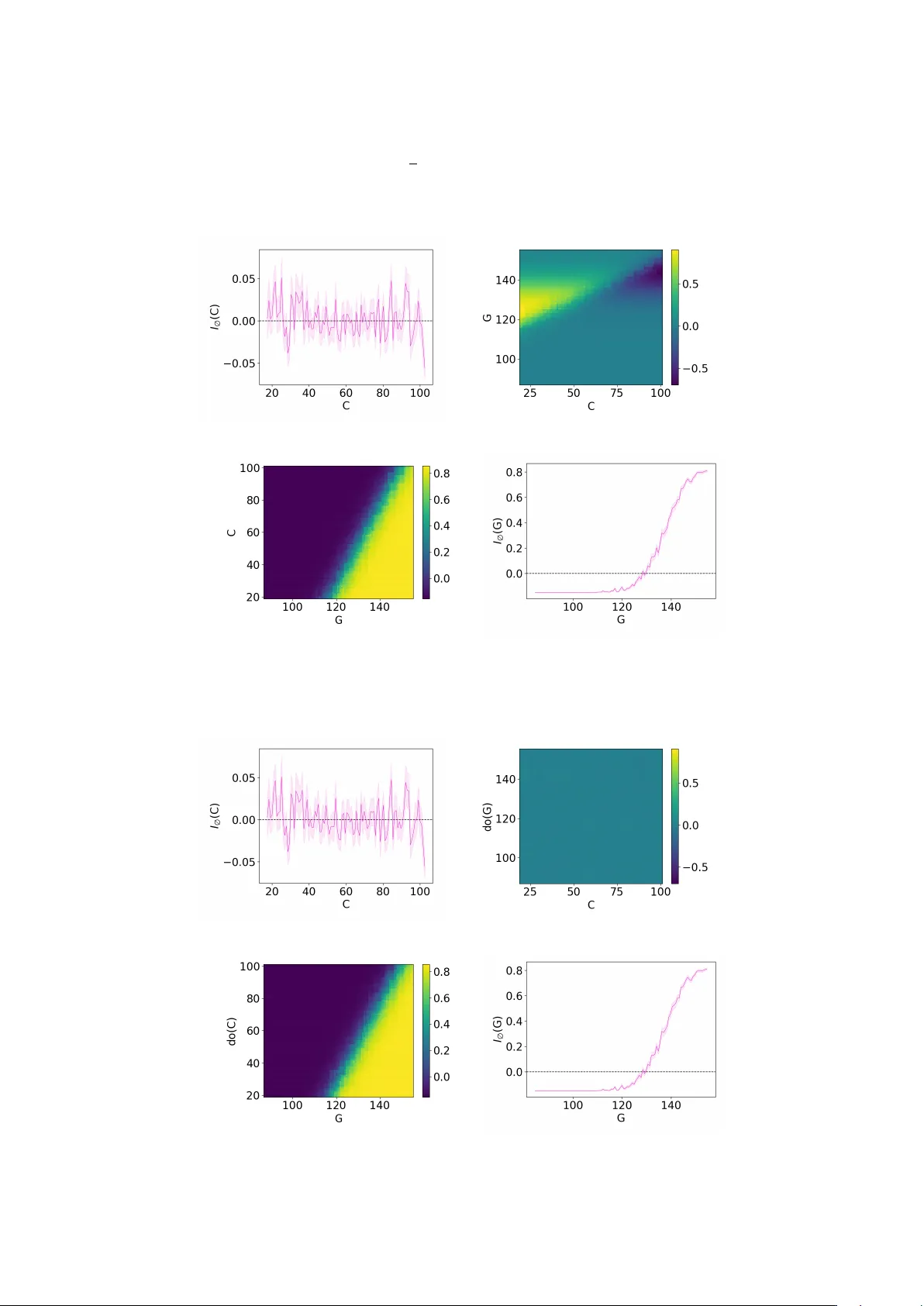
Original Paper
Loading high-quality paper...
Comments & Academic Discussion
Loading comments...
Leave a Comment