Dictionary-based Pathology Mining with Hard-instance-assisted Classifier Debiasing for Genetic Biomarker Prediction from WSIs

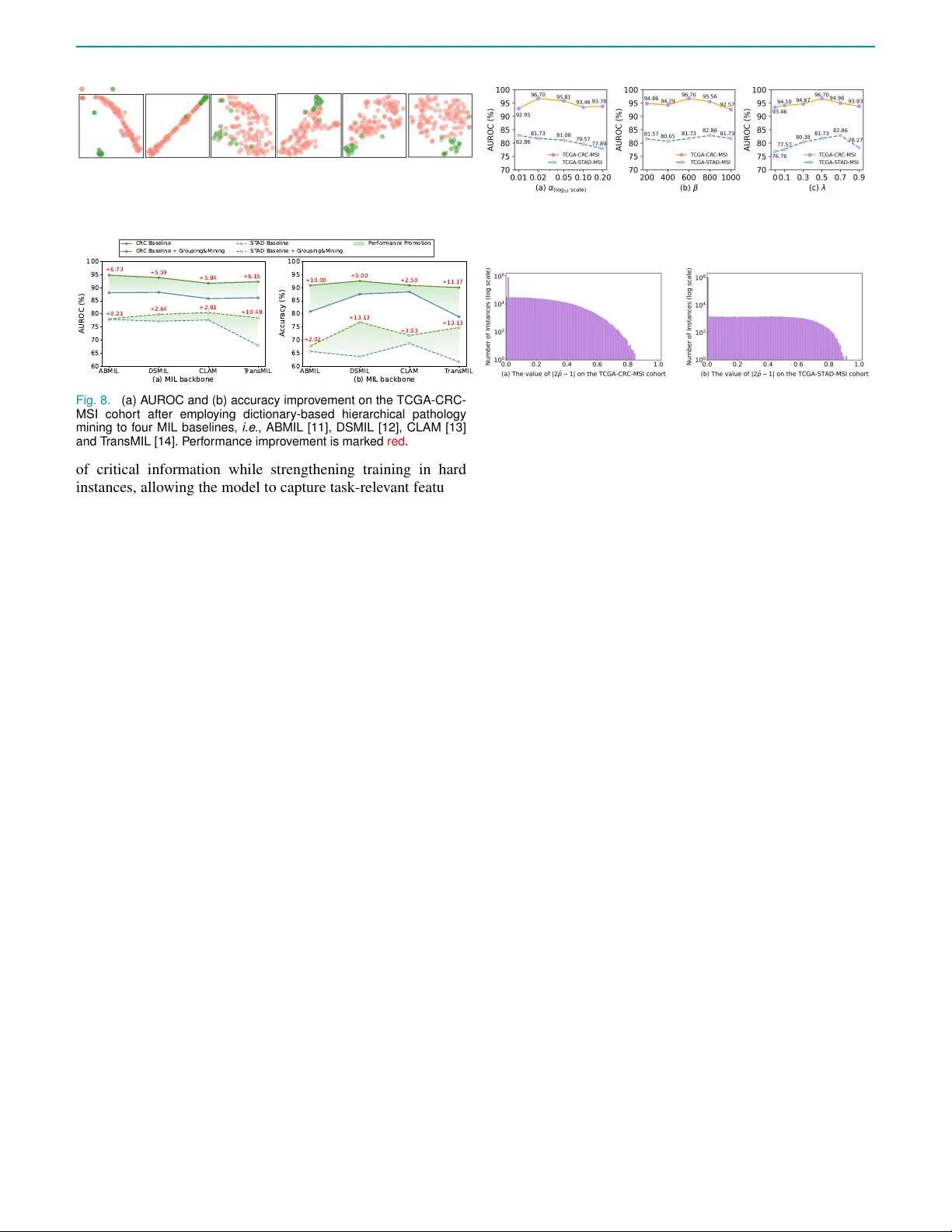
IEEE TRANSACTIONS ON MEDICAL IMA GING, V OL. XX, NO. XX, XXXX 2025 1 Dictionar y-based P athology Mining with Hard-instance-assisted Classifier Debiasing f or Genetic Biomar k er Prediction from WSIs Ling Zhang, Bo xiang Y un, Ting Jin, Qingli Li, Senior Member , IEEE , Xinxing Li, and Y an W ang Abstract — Prediction of genetic biomarkers, e.g. , mi- crosatellite instability in colorectal cancer is crucial for clinical decision making. But, tw o primary challenges ham- per accurate prediction: (1) It is difficult to construct a pathology-aware representation inv olving the complex in- terconnections among pathological components. (2) WSIs contain a large proportion of areas unrelated to genetic biomarkers, which make the model easily overfit simple but irrelative instances. W e hereb y propose a Dictionary- based hierar chical pathology mining with hard-instance- assisted classifier Debiasing framework to address these challenges, dubbed as D 2 Bio. Our first module, dictionary- based hierar chical pathology mining, is ab le to mine di- verse and ver y fine-grained pathological contextual inter- action without the limit to the distances between patches. The second module, hard-instance-assisted classfier debi- asing, learns a debiased classifier via f ocusing on hard but task-related features, without any additional annotations. Experimental results on five cohor ts sho w the superiority of our method, with over 4% impro vement in A UROC com- pared with the second best on the TCGA-CRC-MSI cohort. Our analysis fur ther shows the clinical interpretability of D 2 Bio in genetic biomarker diagnosis and potential clinical utility in survival analysis. Code will be a vailable at https: //github.com/DeepMed- Lab- ECNU/D2Bio . Index T erms — genetic biomarker prediction, whole slide image classification, m ultiple instance learning I . I N T R O D U C T I O N E V ALUA TION of genetic biomarkers is crucial for cancer diagnosis and prognosis, such as microsatellite instability (MSI) and v-raf murine viral oncogene homolog B1 (BRAF) for colorectal cancer and MSI for gastric cancer, since these biomarkers can identify patients with different treatment re- sponse and prognosis [1]–[4]. Specifically , MSI is an impor- tant biomarker for immunotherapy in colorectal and gastric cancers. In contrast, the BRAF mutation, present in about 10% Manuscript submitted on Jan, 2025. This work was supported by the National Natural Science Foundation of China (Grant No. 62471182, 62101191), and Shanghai Rising-Star Prog ram (Grant No. 24QA2702100), and the Science and T echnology Commission of Shanghai Municipality (Grant No . 22DZ2229004). L. Zhang, B. Y un, T . Jin, Q. Li, and Y . W ang are with Shanghai K ey Laboratory of Multidimensional Information Processing, East China Normal University , Shanghai, China (e- mail: zhling@stu.ecnu.edu.cn, 52265904012@stu.ecnu.edu.cn, tjin@stu.ecnu.edu.cn, qlli@cs.ecn u.edu.cn, ywang@cee.ecnu.edu.cn). X. Li is with Depar tment of General Surger y , T ongji Hospital, T ongji Univ ersity School of Medicine, Shanghai 200065, China (e-mail: ahtxxxx2015@163.com). Corresponding author: Y . Wang Negative Positive (a) Atten tion-based m ethod (c) Our d ictionary-bas ed method (b) Grap h-based met hod Convention al graph Dynamic g raph Fig. 1. Motivation of our dictionar y-based strategy . (a) Attention-based MIL methods: simply model the relationships between instances. (b) Graph-based methods: model instance relationships without construc- tion of real pathological components. (c) Proposed dictionar y-based method: utiliz es a learnable dictionar y to g roup instances into patho- logical components and hierarchically mine pathological contextual in- teraction. of colorectal cancer cases, is associated with poor prognosis and poor response to anti-EGFR therapies [5], [6]. T esting genetic biomarkers is time-consuming and expensi ve, with common methods, e .g. , immunohistochemistry , polymerase chain reaction (PCR), and next-generation sequencing [7]. Due to diagnostic needs, whole slide images (WSIs) stained with hematoxylin and eosin (H&E) are routinely a vailable for cancer patients. Besides, previous works [8]–[10] suggest that genetic alterations are expressed in digital pathology WSIs. Therefore, automatically predicting genetic biomakers from WSIs is feasible and highly demanded in clinical practice. Genetic biomark er prediction from gigapixel WSIs is com- monly formulated as a multiple instance learning (MIL) prob- lem, in which only slide-level labels are av ailable, without any patch-lev el annotations. In this setting, each WSI is treated as a bag, and the cropped patches extracted from the slide are regarded as instances, with the learning objectiv e of predicting the corresponding slide-le vel label. Based on this paradigm, a wide range of MIL-based WSI classification methods hav e been developed, including attention-based methods [11]–[15] and graph-based approaches [16]–[18]. Ho we ver , learning bag- lev el genetic biomarker representations and making accurate predictions is challenging. First, constructing a pathology- aware repr esentation including the complex interconnec- tions among pathological components in the tumor micr o- en vironment is difficult. The tumor micro-en vironment in- 2 IEEE TRANSACTIONS ON MEDICAL IMA GING, V OL. XX, NO. XX, XXXX 2025 cludes a rich div ersity of components, e.g . , immune cells, cancer-associated fibroblasts (CAFs), endothelial cells (ECs), pericytes, and other cell types that v ary by tissue—such as adipocytes and neurons, with various pathological com- ponent interactions [19]. For genetic biomarker prediction, mining various pathological component interactions is of great importance [20]. For example, in colorectal cancer , MSI arises from defects in the mismatch repair (MMR) system. This deficiency fails to correct errors occurring during DNA replication (particularly in repetitiv e microsatellite sequences), directly leading to the accumulation of somatic mutations and the subsequent generation of immunogenic neoantigens [21]. This process triggers a robust host immune response, resulting in the e xtensiv e infiltration of T umor -Infiltrating L ymphoc ytes (TILs) into the tumor microen vironment [22]. Similarly , BRAF mutation significantly remodels the tumor microen vironment through di verse pathological interactions. BRAF-mutated tumors, often arising via the serrated neoplasia pathway , are characterized by intense stromal remodeling and specific inflammatory responses [8], [23]. Therefore, these complex spatial interactions among tumor cells, immune cells, and stromal components contain critical discriminativ e infor - mation. Attention-based methods [11]–[15] model the relation- ships between instances to distinguish positi ve from neg ativ e ones by simply merging multiple instance tokens (as depicted in Fig. 1 (a)). These methods struggle to model the complex tumor micro-environment without modeling div erse patholog- ical components. Although HIPT [24] designs a hierarchical transformer-based method, it is still restricted to exploring local pathological information in WSIs. Graph-based methods try to construct the tumor micro-en vironment (as depicted in Fig. 1 (b)). Con ventional graph-based methods [16]–[18] hav e demonstrated impressi ve results, but they construct the tumor micro-en vironment relying on fixed spatial positions, which limits the ability to explore mutual interaction in the tumor micro-en vironment freely . W iKG [25] proposes a dynamic graph representation algorithm to enhance flexible interaction capabilities between instances at arbitrary locations. But it still struggles to represent real pathological components in the tumor micro-en vironment. Second, due to the nature of gigapixel WSIs, they typically contain a large proportion of areas unrelated to genetic biomarkers. While the interconnections be- tween pathological components are learned, the pathology- aware representation still inevitably acquires information that is irrelev ant to genetic biomarkers. Extracting ge- netic biomarkers-related features is like finding a needle in a haystack. The large proportion of irrele vant regions in a WSI makes the model easily overfit simple but irrelativ e instances, ignoring hard b ut task-specific instances (as depicted in Fig. 2). T o solve this problem, instance-level interv entions are introduced. [13] assigns attention-based pseudo labels to several instances to further supervise the model, making the model focus on simple instances and easily overfit task- irrelev ant features. [26] highlights the attention-based “hard- to-classify” instances by masking simple instances, leading to the lost of important information. How to enable the model to focus on hard b ut biomarker classification-relevant features simple hard simple true neg ./pos. instance / original classifier debia sed classifier positive bag negativ e bag task-irrel evant instanc e / Fig. 2. Motivation of our hard-instance-assisted classifier debiasing strategy . Suff erring from redundant task-irrele vant instances, dur ing inference , biased classifier misjudges the bag-lev el labels by ov erfitting simple instances. Lear ning hard instances which include task-specific instances can assist the classifier to reduce the bias. without losing important information is non-tri vial. T o address these issues, we propose a D ictionary-based hi- erarchical pathology mining with hard-instance-assisted clas- sifier D ebiasing method for WSI-based genetic Bio marker pre- diction, dubbed as D 2 Bio. D 2 Bio consists of two modules: (1) dictionary-based hierarchical pathology mining, which learns a pathology-aware representation of WSIs and (2) hard-instance- assisted classifier debiasing, which learns a debiased classifier via focusing on hard but task-related features. Concretely , inspired by sparse dictionary representation [27], which aims to represent a signal using fe wer elements, we introduce a learnable dictionary to construct fine-grained pathological components based on real pathological information in complex WSIs. After constructing pathological components, the hier- archical contextual interaction of intra- and inter -pathological components are extracted and fused (as depicted in Fig. 1 (c)). Compared with attention-based methods [11], [14] and graph- based methods [16], [25], our dictionary-based hierarchical pathology mining enjoys the benefits of completely breaking the limit of instance locations to model the real pathology distribution and extracting hierarchical interaction among fine- grained pathological components in WSIs. Furthermore, we propose a hard-instance-assisted classifier debiasing module to prev ent the classifier from ov erfitting irrelati ve simple informa- tion in WSIs. Specifically , we focus on hard instances in WSIs, and propose an unsupervised clustering strategy to separate positiv e and ne gati ve instances as pseudo labels for training the classifier . Through the dictionary-based hierarchical pathology mining module, a pathology-a ware representation of the WSI is constructed, providing meaningful pathology information to the classifier . Then the classifier enhances its ability to focus on relev ant features through the hard-instance-assisted classifier debiasing module. Thus, we extract comprehensiv e and in-depth biomarker -associated features in WSIs and make robust decisions for genetic biomarker prediction. Extensiv e experiments sho w that our method outperforms all state-of-the- arts. Additionally , our method shows clinical interpretability , providing potential for future clinical applications. The con- tributions of our work are summarized as follo ws: • W e propose a dictionary-based hierarchical pathology mining module which extracts very fine-grained patholog- ical components and explores complex interconnections in WSIs without distance limitation between patches. • W e design a hard-instance-assisted classifier debiasing ZHANG et al. : DICTIONAR Y -BASED P A THOLOGY MINING WITH HARD-INST ANCE-ASSISTED CLASSIFIER DEBIASING FOR GENETIC BIOMARKER PREDICTION FROM WSIS 3 Similarity Matrix Dictionary Key Query   ( ) ( ) 1 F N l l i f  GAP Class token Pathological Groups Pseudo Labels Cluster 1 Clust er 0  1 i c   0 i c  Instance predictions Confident ‘0’ Confident ‘1’ Unconfident Classifier K-means Hard instance set Classifier cluster L     0 , 1 classify L Inter-group ViT Intra-group MSA Intra-group MSA Intra-group MSA Intra-group MSA l -th Ungroup l -th Update Dictionary l -th Group   ( 0) (0 ) 1 F N i f  WSI Image E x t r a c t o r ❄   ( 0) (0 ) 1 F N i f  Fig. 3. Illustration of D 2 Bio . The ov erall framew or k consists of two par ts: 1) dictionar y-based hierarchical pathology mining, 2) hard-instance assisted-classifier debiasing. Giv en a WSI X , our D 2 Bio first initializ e a lear nable dictionar y to extract pathological information of X via cross attention operation. Then our D 2 Bio groups instances into fine-g rained pathological g roups according to the similarity matrix. T o hierarchically mine the interaction, Multi-head Self-attention (MSA) is first employed in each group . Features of X are updated by ungrouping these groups, which is fur ther used to update the dictionar y . After repeating the above steps L times, inter-group ViT is employ ed. Finally , our D 2 Bio assigns hard instance pseudo labels via unsuper vised clustering to super vise the classfication head to reduce the bias in WSIs. The pur ple arrow indicates the classification branch and the orange arro w indicates the classifier debiasing branch. module to learn a robust classifier , prev enting the clas- sifier from overfitting irrelati ve redundant information in WSIs, without any additional annotations. • Extensive experiments on five cohorts demonstrate that our method significantly outperforms mainstream MIL models ( e.g. , with over 4% improvement in A UR OC on the TCGA-CRC-MSI cohort). Our proposed modules can be easily plugged into other MIL methods, offering interpretability and potential usage for survi val analysis. The preliminary version of D 2 Bio, PromptBio [28], was presented as a conference paper at the 27th International Conference on Medical Image Computing and Computer Assisted Intervention (MICCAI 2024). This extended work brings significant improvements: (1) we utilize a learnable dictionary to guide instance grouping instead of prompting large language models; (2) we learn a debiased classifier via focusing on hard but task-related features and (3) we add two ne w cohorts to ev aluate the effecti veness of D 2 Bio, supplemented with extra experiments, ablation studies and clinical analysis. I I . R E L A T E D W O R K A. MIL Methods for WSI Classification Multiple instance learning (MIL) is widely used in whole- slide image (WSI) classification, where WSIs are treated as bags and image patches as instances. MIL methods can be broadly categorized into instance-based and bag-based ap- proaches. Instance-based methods [29]–[31] generate instance predictions and aggregate them to obtain the bag prediction, while bag-based methods [12], [32]–[35] focus on extracting instance features to build bag representations for training a classifier . In bag-based approaches, attention mechanisms [11]–[13] are commonly used to identify k ey instances within WSIs. These methods aim to find a “needle in a haystack” as the positi ve region in WSIs is typically small, and they treat instances as independent entities, overlooking their contextual interactions. More recently , transformer-based methods [14], [15] ha ve been proposed to model inter-instance relation- ships, b ut these methods often merge instance tokens without considering hierarchical contextual interactions within WSIs. Sev eral studies [13], [36]–[39] hav e demonstrated the benefits of instance-lev el supervision for improving bag-le vel classifi- cation performance. For example, [13] assigns pseudo-labels to all instances in negati ve bags and to instances with the highest and lowest attention scores in positi ve bags. [39] utilizes bag- lev el classifiers to generate pseudo-labels for instances, fine- tuning the patch embedder to enhance bag-lev el classification. In [26], hard instances are emphasized by masking simple ones to mitigate bias towards them. In this paper , we focus on hier- archically modeling interactions between di verse pathological components in WSIs and reducing bias of the classifier by unsupervised pseudo-labeling of hard instances. B. Sparse Dictionar y Learning Signal processing techniques commonly require sparse rep- resentations, which capture the useful characteristics of the signal. Sparse representation of a signal in volves the choice of a dictionary , which is the set of atoms used to decompose the signal [27]. Recently sparse dictionary learning has been successfully applied to image analysis, such as image recog- nition [40], [41], denoising [42], [43] and super-resolution [44]–[46]. In the domain of computational pathology , dictio- 4 IEEE TRANSACTIONS ON MEDICAL IMA GING, V OL. XX, NO. XX, XXXX 2025 nary learning has also been utilized for stain normalization [47] and tissue classification using discriminativ e dictionaries built on handcrafted features [48], [49]. In WSIs, there are div erse cellular tissue structures, ranging from coarse-grained (lymphocytes, inflammatory cells, adenocarcinoma, etc. ) to fine-grained (B cells, neutrophils, cancer cells, etc. ). W ithin the fine-grained pathological components, the morphology and size of cells are similar . These both lead to sparsity of gigapixel WSIs. Inspired by sparse dictionary representation, we consider gigapixel WSIs as sparse signals, which can be ef- fectiv ely represented by a dictionary composed of fine-grained pathological components, leading to a dense representation of WSIs. Ho wever , unlike prior pathology methods that construct discriminativ e dictionaries based on handcrafted features and utilizes them primarily for feature reconstruction or sparse coding, our method integrates a learnable dictionary within an end-to-end deep learning framew ork to extract fine-grained pathological components in WSIs, leading to a pathology- aware representation of WSIs. I I I . M E T H O D O L O G Y Mathematically , giv en a WSI X ∈ R W × H × 3 , whose size is W × H , the goal of our task is to predict the image-level label ˆ Y = { 0 , 1 } . Our D 2 Bio consists of two modules: 1) dictionary-based hierarchical pathology mining and 2) hard- instance-assisted classifier debiasing. In the first module, two steps are included, i.e. , dictionary-guided instance grouping and hierarchical interaction mining. Specifically , we first ini- tialize a learnable dictionary D to extract the pathological information of X via cross-attention operation. A lar ge number of atoms in the dictionary can ensure that the dictionary extracts suf ficiently fine-grained pathological information from the WSI. Then we group instances into fine-grained patholog- ical groups according to the similarity between each instance in X and each atom in D . T o mine the interaction within each pathological group, Multi-head Self-Attention (MSA) in each group is first employed. The feature of X is then updated after ungrouping these pathological groups and is subsequently used to update the dictionary . After repeating the abov e steps L times, we obtain pathological groups, which are termed as pathological components. Then inter-group V ision T ransformer (V iT) is employed to mine the interaction among the pathological groups. This dictionary-based hierarchical pathology mining strategy benefits the modeling of a complex and di verse en vironment in WSIs. T o learn a debiased binary classifier for differentiating between positiv e and negati ve instances, we further assign hard instance pseudo labels via unsupervised clustering, which is utilized to assist the classi- fication head to identify important underlying entities that are difficult to discern. A. Problem F or mulation In a binary classification task based on the multiple instance learning setting, a WSI is considered as a bag and the patches cropped from the WSI are regarded as instances. The bag is negati ve only when all instances are negativ e, and the bag is positiv e when at least one instance is positiv e. W e consider the prediction of genetic biomarkers based on WSIs as a bag- lev el classification task, where only the bag label Y ∈ { 0 , 1 } is av ailable. The feature of the i -th instance is obtained through feeding the i -th cropped patch into a frozen image extractor , denoted as f (0) i ∈ R d , where d is the dimension of the feature. B. Dictionar y-based Hierarchical P athology Mining 1) Dictionar y-Guided Instance Grouping : Sparse dictionary representation [27] is a form of representation learning which originated in signal processing. It aims to represent a signal using fewer elements, and through dictionary learning, it can effecti vely enhance the sparsity of the signal. The assumption of dictionary learning is that gi ven a signal set S = { s i } ˙ N i =1 ∈ R ˙ d × ˙ N , where ˙ d is the dimension of a single signal and ˙ N is the number of signals, we hope to find a dictionary ˙ D = h ˙ d 1 , ˙ d 2 , . . . , ˙ d ˙ K i ∈ R ˙ d × ˙ K , where each of the dictionary’ s columns is an atom and ˙ K is the number of atoms, and an expression E ∈ R ˙ K × ˙ N , subject to S ≃ ˙ DE , to seek the sparse representation. When ˙ K < ˙ d , the dictionary is an undercomplete dictionary . More precisely , a sparse dictionary problem can be viewed as the following optimization problem: min ˙ D ∈D , E ∈E    S − ˙ DE    2 F , (1) where ∥·∥ F means the Frobenius norm, and D and E are possible sets of the dictionaries and e xpressions. Most sparse dictionary learning methods perform a two- stage procedure iteratively to choose the dictionary: start with an initial dictionary and repeat the follo wing two stages ( e .g. , Eq. (2) and Eq. (3)) sev eral times. Stage 1 uses the current dictionary to find the sparse expression and stage 2 updates the dictionary to reduce the error of stage 1. Stage 1 Sparse representation: E ( l +1) = argmin E ∈E    S − ˙ D ( l ) E ( l )    2 F . (2) Stage 2 Dictionary updating: ˙ D ( l +1) = argmin ˙ D ∈D    S − ˙ D ( l ) E ( l +1)    2 F . (3) where l is the number of updates. Inspired by sparse dictionary learning, we consider a WSI as an input sparse signal, which contains substantial instances. W e establish a dictionary to densely represent the WSI and extract pathological components in this section. W e first ini- tialize a dictionary D (0) = h d (0) 1 , d (0) 2 , . . . , d (0) K i ∈ R K × d , which includes K atoms of dimension d . T o densely represent the WSI, we set K < d . W e aim to learn a specific and comprehensiv e representation of the WSI using the dictionary . Therefore, we treat the WSI features F (0) ∈ R N × d , consisting of N instances and the i -th instance feature is f (0) i , as the query , and treat the initialized dictionary D (0) as the key to extract pathological information in the WSI: e Q (0) = F (0) · W Q , e K (0) = D (0) · W K , (4) where W q ∈ R d × r and W k ∈ R d × r project inputs to a lower dimension ( r = 4 ) for ef ficient attention computation. ZHANG et al. : DICTIONAR Y -BASED P A THOLOGY MINING WITH HARD-INST ANCE-ASSISTED CLASSIFIER DEBIASING FOR GENETIC BIOMARKER PREDICTION FROM WSIS 5 Then we calculate the similarity between e Q (0) and e K (0) : H (0) = Softmax  sim  e Q (0) , e K (0)  /γ  , (5) where sim( · , · ) refers to cosine similarity and γ is a parameter to adjust the similarity range. This giv es the similarity H (0) ∈ R N × K between each instance feature in F (0) and each atom in the dictionary D (0) . Then we aim to construct explicit pathological groups to model the div erse fine-grained pathological components in WSIs. W e group instances into K pathological compo- nents, i.e. , { P (0) k } K k =1 , based on the similarity H (0) (see Eq. (6)). Specifically , if h (0) ik is the maximum similarity in { h (0) i 1 , h (0) i 2 , . . . , h (0) iK } , where h (0) ik is the similarity between the i -th instance feature f (0) i and the k -th atom in D (0) , then the instance feature f (0) i is assigned to the k -th group P (0) k : P (0) k =  f (0) i | arg max j  h (0) ij  = k  N i =1 , (6) where k , j ∈ { 1 , 2 , ..., K } . In this way , each instance can be assigned to the corre- sponding pathological group based on its similarity to the atoms in the dictionary . But, this grouping process results in varying numbers of instances in each pathological group, making parallel computation difficult. T o obtain balanced pathological groups, all pathological groups { P (0) k } K k =1 are flattened, concatenated and redivided into G pathological groups, i.e. , { ˙ P (0) g } G g =1 , where each pathological group has the same number of instances. In the above steps, we record the position information for each instance. In this way , we group all instances of the WSI into G pathological components based on the learnable dictionary . After the grouping, we propose an intra-group interaction mining strategy , whose details will be introduced in Sec. III- B.2. Then we ungroup all pathological components to update the WSI features, i.e. , F (1) , based on the recorded position information for each instance. Following sparse dictionary learning, we use F (1) and the similarity H (0) to update the dictionary , followed by setting a parameter τ for further mo- mentum updating the dictionary D (0) . It is important to note that before this ungrouping, the grouped features hav e already been processed by the Intra-group MSA (detailed in Sec. III- B-2) and aggregated via Global A verage Pooling (GAP) to generate features of pathological components. These features are preserved for the subsequent Inter-group V iT , ensuring that the semantic structure is fully leveraged rather than discarded, while ungrouping allows the instance features to be realigned with the similarity matrix for dictionary refinement. Thus, we obtain an updated dictionary D (1) . W e repeat the above process for L times, which can be formulated as below: ˆ D ( l ) = Softmax  Norm  H ( l ) ⊤  · F ( l ) , (7) D ( l +1) = τ ˆ D ( l ) + (1 − τ ) D ( l ) , (8) where l ∈ { 1 , 2 , ..., L } , Softmax( · ) and Norm( · ) indicate softmax and instance norm operations, respectively . τ is a learnable parameter initialized to 0. MSI Cancer Sli de Pr ediction Map MSS Cancer Sli de Prediction Map MSS MSI MSI Patterns lymphocytic infiltration aggregated lymphocytes aggregated tumor cells MSS Patterns sparse lymphocytes sparse plasma cells MSS MSI Fig. 4. Heatmap visualization of D 2 Bio on the MSI prediction task and identified pathological patterns. 2) Hierarchical Interaction Mining : In this section, we in- troduce hierarchically mining contextual interaction of intra- and inter-pathological components. For interaction of intra- pathological components, v arious interaction occur among lymphocytes to regulate immune responses, forming a com- plex immune network. As for interaction of inter-pathological components, lymphocytes and inflammatory cells interact through signaling molecules and chemical mediators to reg- ulate the intensity of immune responses. Therefore, mining interaction of intra- and inter -pathological components counts a lot for modeling the tumor micro-en vironment. T o mine the interaction within each fine-grained patholog- ical component ˙ P ( l ) g , where g = { 1 , 2 , ..., G } , we conduct intra-group MSA operation on all the instance features in ˙ P ( l ) g : ¨ P ( l ) g = MSA  ˙ P ( l ) g · W q , ˙ P ( l ) g · W k , ˙ P ( l ) g · W v  , (9) where W q ∈ R d × r and W k ∈ R d × r project inputs to a lower dimension ( r = 4 ) to compute attention scores efficiently , while W v ∈ R d × d maintains the full feature dimension. After conducting MSA operation within each fine-grained pathological component and updating the dictionary L times, we separately aggregate the instance features of each patho- logical group by global average pooling and obtain all the features of pathological component, i.e . , { ¯ P g } G g =1 . Then, we concatenate a class tok en CLS ∈ R d with all the group features. The concatenated feature is further fed into the inter-group V iT layer to mine the interaction among all the pathological groups. W e use a Multi-Layer Perception (MLP) head to map the output class token CLS ′ ∈ R d to the final class probability ˆ P . So far , we design a simple yet effecti ve dictionary-based hierarchical pathology mining strate gy . W e use the genetic biomarker label Y ∈ { 0 , 1 } to supervise the classification head. The cross-entropy loss is adopted for calculating the classification loss: L cls = CELoss  ˆ P , Y  . (10) C . Hard-Instance-Assisted Classifier Debiasing Due to the complexity and di versity of biological phenom- ena, many phenotypic features in WSIs are not absolutely specific, leading to inherent bias in the dataset. With the bias, the model easily overfits simple instances and relies on 6 IEEE TRANSACTIONS ON MEDICAL IMA GING, V OL. XX, NO. XX, XXXX 2025 T ABLE I C O M P A R I S O N S W I T H S T ATE - O F - T H E - A R T M I L M E T H O D S O N FI V E C O H O R T S U S I N G T W O F E ATU R E E X T R A C TO R S , i.e. , C T R A N S P A T H [ 5 0 ] A N D U N I V 2 [ 5 1 ] . W E R E P O RT M E A N ( 9 5 % C I ) I N P E R C E N TAG E ( % ) . “ * ” D E N O T E S S TA T I S T I C A L S I G N I FI C A N C E ( P < 0 . 0 5 ) . B E S T R E S U LT S A R E S H OW N I N B O L D . CtransPath [50] Method TCGA-CRC-MSI TCGA-CRC-BRAF CPT AC-MSI CPT AC-BRAF TCGA-ST AD-MSI A UC Acc PRC Bal A UC Acc PRC Bal A UC Acc PRC Bal AUC Acc PRC Bal AUC Acc PRC Bal ABMIL [11] 88.00 ∗ 80.80 ∗ 64.80 86.20 68.40 ∗ 80.80 24.80 54.90 ∗ 87.50 76.20 ∗ 49.10 50.00 ∗ 85.20 85.70 ∗ 56.90 50.00 ∗ 77.80 65.70 ∗ 46.80 ∗ 67.80 ∗ (75.5-96.6) (73.3-87.5) (46.0-83.1) (77.6-92.4) (46.1-87.6) (74.2-87.5) (6.4-55.7) (41.5-71.0) (68.8-100.0) (76.2-76.2) (29.8-100.0) (50.0-50.0) (72.6-99.4) (85.7-85.7) (21.8-95.8) (50.0-50.0) (67.8-87.2) (56.6-74.7) (35.2-68.2) (57.7-77.8) DSMIL [12] 88.20 ∗ 87.50 ∗ 62.70 81.40 63.80 ∗ 76.70 ∗ 24.70 52.70 ∗ 91.20 76.20 57.30 56.90 ∗ 87.00 85.70 38.80 50.00 77.10 63.60 ∗ 47.70 ∗ 63.80 ∗ (76.1-97.5) (81.7-93.3) (40.2-87.9) (68.6-92.4) (40.5-83.8) (70.0-83.3) (5.6-56.8) (39.3-69.2) (76.2-100.0) (61.9-85.7) (34.4-100.0) (40.6-76.9) (78.1-92.2) (85.7-85.7) (22.1-75.2) (50.0-50.0) (66.7-86.6) (54.5-72.7) (35.2-69.3) (53.1-73.8) CLAM-SB [13] 85.80 ∗ 88.30 69.80 84.80 70.00 ∗ 76.70 ∗ 33.60 64.30 90.00 81.00 55.50 80.60 77.80 85.70 ∗ 50.10 63.90 ∗ 77.60 68.70 ∗ 47.70 ∗ 69.80 ∗ (72.0-97.1) (82.5-94.2) (47.3-88.1) (73.8-94.3) (48.9-88.2) (69.2-84.2) (6.8-62.3) (46.9-83.0) (73.8-100.0) (61.9-95.2) (33.0-100.0) (60.0-96.9) (70.4-88.9) (81.4-90.5) (31.6-73.7) (48.9-79.2) (67.4-87.2) (59.6-77.8) (35.8-68.6) (59.1-79.8) TransMIL [14] 83.70 ∗ 80.00 ∗ 52.20 ∗ 77.10 62.60 ∗ 70.00 ∗ 26.60 60.70 88.70 81.00 55.80 80.60 92.60 85.70 ∗ 67.80 50.00 ∗ 67.90 ∗ 61.60 ∗ 47.30 62.40 ∗ (70.4-94.3) (73.3-86.7) (30.2-79.0) (65.2-88.1) (38.9-85.3) (61.7-78.3) (5.7-58.8) (42.9-78.6) (71.3-100.0) (61.9-95.2) (32.1-100.0) (57.5-96.9) (78.9-99.3) (85.7-85.7) (36.4-96.4) (50.0-50.0) (56.5-79.2) (52.5-71.7) (31.8-63.8) (51.7-73.1) DTFD [35] 84.19 ∗ 85.00 ∗ 58.47 ∗ 77.15 70.54 ∗ 79.17 ∗ 26.79 54.02 ∗ 87.50 ∗ 76.20 ∗ 59.26 ∗ 50.00 ∗ 87.00 ∗ 85.70 ∗ 62.50 ∗ 50.00 ∗ 75.40 ∗ 65.70 ∗ 45.60 ∗ 70.40 (72.6-95.8) (78.3-90.8) (34.2-79.6) (63.8-89.5) (52.4-86.9) (72.5-85.8) (7.1-55.4) (40.2-70.1) (70.0-100.0) (76.2-76.2) (29.6-100.0) (50.0-50.0) (70.4-88.7) (85.7-85.7) (46.1-73.7) (50.0-50.0) (64.7-84.8) (56.6-74.7) (34.1-66.5) (60.4-79.1) HIPT [24] 83.90 ∗ 74.20 ∗ 61.80 76.70 72.80 68.30 ∗ 40.00 71.40 88.80 76.20 ∗ 67.10 70.60 ∗ 92.60 81.00 ∗ 67.80 75.00 79.60 62.60 ∗ 54.20 72.40 (70.4-94.7) (66.7-81.7) (38.7-81.6) (65.7-86.2) (46.0-95.5) (60.0-76.7) (10.4-74.8) (54.9-85.7) (71.3-100.0) (57.1-90.5) (32.3-100.0) (46.8-93.8) (87.4-99.6) (76.7-90.0) (36.2-97.6) (60.0-91.7) (69.7-88.7) (53.5-70.7) (39.6-75.7) (64.3-79.7) MHIM-MIL [26] 83.00 ∗ 85.83 ∗ 56.42 ∗ 77.62 74.90 76.67 ∗ 24.50 75.89 92.50 81.00 72.45 80.63 88.05 85.71 ∗ 59.24 77.78 66.11 ∗ 49.49 ∗ 34.56 ∗ 56.95 ∗ (71.5-94.6) (79.2-91.7) (32.2-81.1) (64.3-89.3) (56.1-93.7) (68.3-84.2) (08.5-52.2) (54.2-91.0) (80.8-100) (61.9-95.2) (35.4-100) (60.6-96.9) (66.2-92.6) (66.7-95.2) (18.5-100) (52.8-94.4) (54.2-78.0) (39.4-59.6) (21.1-51.2) (46.8-67.1) W iKG [25] 90.20 ∗ 90.00 67.30 82.90 80.20 67.50 ∗ 17.20 76.80 92.50 90.50 77.50 93.80 92.60 85.70 65.60 91.70 79.80 70.70 ∗ 54.10 64.50 ∗ (81.5-97.2) (84.2-95.0) (43.8-89.5) (70.5-93.3) (67.9-90.7) (59.2-75.8) (9.6-51.3) (62.1-86.6) (77.5-100.0) (76.2-100.0) (39.7-100.0) (84.4-100.0) (93.1-100.0) (81.4-95.2) (80.5-100.0) (89.2-97.2) (70.3-88.4) (62.6-79.8) (39.2-76.5) (53.8-75.2) PromptBio [28] 91.80 ∗ 86.70 ∗ 45.90 ∗ 63.80 ∗ 80.10 70.00 ∗ 30.90 72.30 93.80 90.50 62.70 86.90 92.60 71.40 ∗ 65.60 83.30 77.00 73.70 43.60 ∗ 66.50 ∗ (86.1-96.1) (81.7-91.7) (31.9-73.4) (51.4-76.7) (61.3-94.1) (61.7-78.3) (10.2-62.1) (54.9-86.2) (81.2-100.0) (76.2-100.0) (38.7-100.0) (66.9-100.0) (79.3-96.1) (48.6-80.0) (25.2-83.1) (70.0-88.3) (67.2-86.3) (65.7-81.8) (32.9-62.6) (55.9-77.2) D 2 Bio (ours) 96.70 92.50 72.20 75.70 83.80 85.80 20.90 63.40 96.30 90.50 86.00 86.90 94.40 95.20 81.70 83.30 81.70 77.80 59.00 77.20 (93.1-99.4) (88.3-95.8) (50.7-97.1) (62.9-88.6) (74.3-92.4) (80.0-90.8) (11.4-54.6) (46.0-81.7) (85.0-100.0) (76.2-100.0) (48.3-100.0) (66.9-100.0) (76.1-100.0) (91.0-100.0) (50.9-100.0) (68.3-100.0) (71.9-90.6) (69.7-85.9) (42.7-77.7) (67.2-86.5) UNI v2 [51] Method TCGA-CRC-MSI TCGA-CRC-BRAF CPT AC-MSI CPT AC-BRAF TCGA-ST AD-MSI A UC Acc PRC Bal A UC Acc PRC Bal A UC Acc PRC Bal A UC Acc PRC Bal AUC Acc PRC Bal ABMIL [11] 93.30 ∗ 90.00 ∗ 63.90 ∗ 82.90 88.30 ∗ 92.50 38.60 ∗ 72.80 93.80 ∗ 90.50 ∗ 62.70 ∗ 86.90 ∗ 94.10 85.70 73.10 81.60 81.60 68.70 ∗ 56.10 71.10 ∗ (86.8-98.2) (84.2-95.0) (43.3-91.8) (70.5-93.8) (69.6-93.9) (92.5-94.8) (20.8-46.2) (55.9-78.1) (76.2-93.1) (72.9-90.0) (35.6-58.3) (69.1-86.6) (94.3-100.0) (81.9-99.5) (76.5-100.0) (70.7-99.7) (71.8-90.1) (59.6-77.8) (40.7-75.9) (61.0-79.8) DSMIL [12] 89.20 ∗ 90.80 ∗ 58.90 ∗ 71.90 ∗ 73.10 ∗ 75.80 ∗ 38.30 63.80 ∗ 93.80 90.50 62.70 86.90 95.60 90.50 83.50 84.60 ∗ 84.10 74.70 ∗ 61.40 76.50 (78.7-96.5) (86.7-95.0) (37.6-82.5) (59.0-85.2) (46.6-84.1) (67.1-79.7) (14.2-53.7) (47.6-71.4) (88.1-99.4) (81.9-94.8) (50.0-96.2) (74.4-95.9) (92.8-99.4) (85.7-94.3) (77.4-98.7) (81.6-86.9) (73.4-93.1) (66.6-82.8) (46.2-85.2) (66.4-85.2) CLAM-SB [13] 94.00 ∗ 83.30 ∗ 87.60 71.50 ∗ 83.80 85.00 ∗ 74.60 28.40 95.00 90.50 93.80 77.70 91.20 ∗ 85.70 81.60 51.90 ∗ 78.60 ∗ 68.70 ∗ 71.10 ∗ 57.10 ∗ (86.7-98.9) (76.7-90.0) (79.5-93.8) (49.4-93.4) (78.3-98.2) (78.6-89.9) (61.2-93.3) (19.2-67.1) (88.2-99.6) (86.2-99.5) (90.9-99.7) (51.7-98.6) (88.2-98.4) (81.0-94.8) (61.5-93.5) (42.6-94.0) (68.1-88.1) (59.6-77.8) (61.1-81.1) (40.7-73.5) TransMIL [14] 90.20 ∗ 82.50 ∗ 84.30 ∗ 48.20 ∗ 77.60 ∗ 81.70 ∗ 72.80 36.30 95.00 81.00 66.90 ∗ 77.70 89.70 76.20 ∗ 75.70 ∗ 50.10 84.50 80.80 73.90 55.60 ∗ (82.5-96.3) (75.0-89.2) (74.3-92.4) (32.4-78.3) (61.5-87.9) (76.2-88.1) (49.4-86.3) (19.9-69.7) (95.5-100.0) (76.7-90.0) (57.2-79.0) (79.6-100.0) (88.8-100.0) (76.7-90.0) (79.3-93.8) (42.8-100.0) (76.1-91.8) (72.7-87.9) (63.8-84.6) (41.6-76.8) DTFD [35] 95.90 ∗ 93.30 90.50 72.60 ∗ 84.30 ∗ 85.80 ∗ 80.80 42.90 96.30 90.50 86.90 86.00 85.30 ∗ 81.00 ∗ 88.20 ∗ 39.90 ∗ 82.80 75.80 ∗ 75.80 65.50 (90.3-99.6) (89.2-97.5) (80.5-98.1) (52.9-98.0) (60.4-87.0) (81.1-86.6) (62.8-86.5) (21.3-59.1) (89.1-99.7) (77.1-99.5) (71.9-99.7) (72.1-99.2) (76.6-89.7) (67.1-85.2) (79.7-90.9) (29.3-45.9) (72.9-91.2) (66.7-83.8) (65.2-85.8) (49.2-80.7) HIPT [24] 94.60 ∗ 87.50 ∗ 87.10 ∗ 67.40 ∗ 77.30 ∗ 82.50 ∗ 73.20 27.80 93.80 ∗ 90.50 93.80 62.70 ∗ 91.20 85.70 91.20 51.90 78.70 ∗ 77.80 ∗ 77.20 51.60 ∗ (89.3-98.5) (81.7-93.3) (77.1-95.2) (45.4-91.0) (56.5-92.9) (80.2-85.0) (66.2-85.6) (18.1-61.9) (75.0-93.1) (76.7-90.0) (84.7-93.4) (33.9-58.1) (79.3-100.0) (72.9-90.5) (83.2-94.1) (33.0-100.0) (68.4-87.7) (69.7-85.9) (67.1-86.5) (37.0-67.9) MHIM-MIL [26] 94.90 ∗ 86.70 ∗ 49.50 ∗ 63.90 ∗ 82.00 ∗ 92.50 61.20 25.50 ∗ 95.00 85.70 76.90 ∗ 77.70 82.40 81.00 50.00 ∗ 80.60 79.50 75.80 ∗ 67.90 ∗ 51.00 ∗ (88.8-98.9) (85.0-87.5) (48.6-50.0) (44.9-92.8) (79.4-92.4) (90.1-91.7) (54.1-65.9) (17.9-30.7) (92.6-100.0) (85.7-94.8) (71.4-89.7) (51.2-100.0) (65.0-100.0) (81.0-81.0) (50.0-50.0) (59.9-100.0) (70.0-88.6) (67.7-83.8) (57.2-78.6) (37.7-72.2) W iKG [25] 95.50 ∗ 94.20 82.40 ∗ 67.10 ∗ 85.00 ∗ 90.80 ∗ 54.50 ∗ 25.10 ∗ 96.30 71.40 ∗ 81.20 ∗ 86.00 94.10 90.50 94.10 57.90 75.40 ∗ 75.80 73.20 47.10 ∗ (90.6-98.9) (90.0-97.5) (69.5-93.3) (46.0-94.2) (79.4-94.5) (86.2-93.2) (46.8-60.2) (17.8-40.1) (90.0-100.0) (62.9-76.2) (75.6-84.4) (63.9-100.0) (83.5-100.0) (86.2-100.0) (91.5-100.0) (37.7-100.0) (64.9-85.5) (67.7-83.8) (63.1-83.2) (34.0-65.3) PromptBio [28] 96.80 91.70 ∗ 75.20 ∗ 69.20 90.20 ∗ 72.50 ∗ 79.50 31.80 95.00 76.20 ∗ 50.00 ∗ 77.70 85.30 ∗ 81.00 78.70 ∗ 42.30 ∗ 81.40 ∗ 77.80 67.90 ∗ 50.50 ∗ (93.4-99.2) (87.5-95.8) (62.4-88.6) (49.0-95.4) (81.6-93.1) (69.3-74.1) (67.1-85.7) (21.7-52.4) (93.9-100.0) (76.2-76.2) (50.0-50.0) (64.0-100.0) (69.3-95.1) (67.1-90.5) (63.9-84.6) (24.6-83.7) (71.5-90.0) (69.7-84.8) (57.2-78.0) (37.3-72.1) D 2 Bio (ours) 98.50 96.70 87.50 92.40 92.60 94.20 52.60 73.70 97.50 90.50 93.80 93.80 97.10 90.50 87.10 94.10 86.20 82.80 70.90 80.60 (96.2-100.0) (93.3-99.2) (69.0-100.0) (82.4-99.5) (87.7-94.2) (94.2-95.8) (43.6-61.4) (68.8-79.0) (96.4-100.0) (85.7-94.8) (92.1-100.0) (90.6-96.6) (94.1-100.0) (77.1-90.5) (44.0-100.0) (85.9-94.1) (76.1-93.7) (74.7-89.9) (54.1-85.5) (70.5-88.6) non-specific features, leading to misclassification. Therefore, instead of only learning simple instances, we focus on learning hard instances, identifying underlying patterns that are difficult to discern b ut truly relev ant to the label. Specifically , we feed all the original instance features F (0) = { f (0) 1 , f (0) 2 , . . . , f (0) N } into the final classification head C , outputting the prediction logits of each instance ˆ p i as follo ws: ˆ p i = Sigmoid  C  f (0) i  , i ∈ { 1 , 2 , . . . , N } , (11) where Sigmoid( · ) means the sigmoid operation. If the difference between ˆ p i and 1 − ˆ p i is too small, we collect f (0) i into the hard instance set T as follows: T = n f (0) i | | ˆ p i − (1 − ˆ p i ) | < α o N i =1 , (12) where i ∈ { 1 , 2 , . . . , N } and α is the hard threshold. When the number of hard instances in the WSI is greater than β (threshold for the number of hard instances), we focus on mining the intrinsic dif ference in the hard instance set to distinguish task-specific and task-irrele vant features. W e assign pseudo labels to these hard instances in T via unsupervised clustering, e.g . , K-means algorithm. After clustering these hard instances into two clusters, we use the cluster label c i ∈ { 0 , 1 } to supervise the classification head C to learn from these hard instances. T o ensure the cluster labels generated by unsuper- vised clustering are task-relev ant, we employ a prediction- guided alignment strategy . For hard instances deri ved from negati ve bags, we assign a negati ve label ( c i = 0 ) to both two clusters U 0 and U 1 as they are guaranteed to be ne gativ e. For hard instances deriv ed from positive bags, we calculate the average prediction score ¯ p k = 1 |U k | P f (0) i ∈U k ˆ p i for each cluster k ∈ { 0 , 1 } , where ˆ p i is the prediction logit of feature f (0) i . If ¯ p 0 < ¯ p 1 , we assign the pseudo-label 0 to instances in U 0 and 1 to those in U 1 , and vice versa. This strategy lev erages the collective confidence of the classifier to correct individual noisy predictions. This unsupervised mining can prevent the classifier from ov erfitting task-irrelev ant features. ZHANG et al. : DICTIONAR Y -BASED P A THOLOGY MINING WITH HARD-INST ANCE-ASSISTED CLASSIFIER DEBIASING FOR GENETIC BIOMARKER PREDICTION FROM WSIS 7 T ABLE II A B L A T I O N S T U DY O F T W O K E Y C O M P O N E N T S O N T C G A - C R C - M S I C O H O R T . W / O M I N I N G : A L L I N S TAN C E S A R E F E D I N T O T W O V I T L AYE R S W I T H O U T D I C T I O N A RY - G U I D E D I N S TAN C E G R O U P I N G . T H E S Y M B O L “ * ” I N D I C ATE S O N L Y I N T E R - G R O U P I N T E R AC T I O N M I N I N G I S C O N D U C T E D W I T H O U T I N T R A - G RO U P I N T E R A C T I O N M I N I N G . W / O D E B I A S I N G : R E M OV E T H E H A R D - I N S T A N C E - A S S I S T E D C L A S S I FI E R D E B I A S I N G M O D U L E . Pathology Mining Debiasing TCGA-CRC-MSI TCGA-ST AD-MSI × × 88.63 64.05 × ✓ 91.49 79.73 * × 88.70 64.32 ✓ × 93.46 80.00 ✓ ✓ 96.70 81.73 The debiasing loss can be formulated as: L debias = 1 t t X i CELoss ( ˆ p i , c i ) , (13) where t is the number of hard instances in T . The total loss is calculated as: L = L cls + λ · L debias , (14) where λ is a weight in the loss function to balance the debiasing loss and classifying loss. I V . E X P E R I M E N T A L R E S U L T S A. Datasets TCGA-CRC dataset. The Cancer Genome Atlas [52] colorectal cancer dataset (TCGA-CRC) [53] includes two subtypes: microsatellite stable (MSS) and microsatellite insta- bility (MSI), collecti vely referred to as the TCGA-CRC-MSI cohort, as well as BRAF mutation and non-BRAF mutation, collectiv ely referred to as the TCGA-CRC-BRAF cohort. The TCGA-CRC-MSI cohort consists of 420 MSS slides and 62 MSI slides, while the TCGA-CRC-BRAF cohort contains 429 non-BRAF slides and 53 BRAF slides. Each cohort is randomly di vided into training and testing sets in a 3:1 ratio, with 10% of the training set further allocated as the validation set. CPT A C-COAD dataset. The Clinical Proteomic T umor Analysis Consortium colon adenocarcinoma dataset (CPT A C- CO AD) [54], hosted on The Cancer Imaging Archiv e (TCIA) [55], includes two cohorts: CPT A C-COAD-MSI and CPT A C- CO AD-BRAF . The CPT A C-CO AD-MSI cohort contains 81 MSS slides and 24 MSI slides, while the CPT AC-CO AD- BRAF cohort consists of 16 BRAF slides and 90 non-BRAF slides. This dataset is randomly split into training, validation, and testing sets in a 3:1:1 ratio. TCGA-ST AD dataset. The TCGA stomach adenocarcinoma dataset (TCGA-ST AD) [56] includes 224 MSS slides and 60 MSI slides, collecti vely referred to as the TCGA-ST AD-MSI cohort. Preprocessed patches from all slides, as provided in [8], are utilized in this study . W e follow the data split strategy in [8], dividing the dataset into training and testing sets and reserving 10% of the training set as the validation set. All data (including histological images) from the TCGA database are av ailable at https: //portal.gdc.cancer.gov/ . All data from the T ABLE III A B L A T I O N S T U DY O F G R O U P I N G S T R ATE G I E S O N T H E T C G A - C R C - M S I A N D T C G A - S T A D - M S I C O H O R T S . R A N D . : R A N D O M L Y D I V I D I N G I N S T A N C E S . K - M E A N S : C L U S T E R I N G I N S TA N C E S U S I N G K - M E A N S . T E X T : U S I N G G P T - 4 TO G E N E R A T E A S M A N Y D E S C R I P T I O N S A S P O S S I B L E , i.e. , 1 5 D E S C R I P T I O N S A N D G R O U P I N G I N S T A N C E S I N TO 1 5 G RO U P S F O L L O W I N G [ 2 8 ] . K - N N ( D I S T ) : K - N N G R O U P I N G B A S E D O N E U C L I D E A N D I S T A N C E . K - N N ( C O S ) : K - N N G R O U P I N G B A S E D O N C O S I N E S I M I L A R I T Y . D I C . : D I C T I O N A RY - G U I D E D G R O U P I N G . T H E B E S T R E S U L T F O R E A C H C O H O R T I S H I G H L I G H T E D . Cohort Rand. T ext K-means k-NN (dist) k-NN (cos) Dic. TCGA-CRC-MSI 89.46 91.75 92.83 92.00 90.86 96.70 TCGA-ST AD-MSI 78.97 78.70 75.62 65.73 66.49 81.73 ... Group 1 Group 2 Group 61 Group 60 Group 120 ... Original Slide of MSI Cance r Grouping Map Group 1 Group 120 Lymphocytic infiltration Lymphocytes Tumor cells Tumor cells Adipocytes Fig. 5. P athological group distribution and corresponding pathological patterns on a WSI of MSI cancer. CPT A C cohort are av ailable at https://proteomic. datacommons.cancer.gov/ . All clinical data for patients in the TCGA and CPT A C cohorts are av ailable at https://cbioportal.org/ . W e strictly conduct patient-lev el splitting across all datasets. F or patients containing multiple slides in the raw cohorts, we select a single slide (typically the diagnostic slide, DX) for each patient to construct the experimental cohorts, ensuring no patient ov erlap across the subsets. B. Evaluation Metrics For all cohorts, we ev aluate the performance of different methods with four metrics, i.e. , Area Under Receiv er Operator Curve Score (A UROC) (%), Accuracy (%), Area Under the Precision–Recall Curve (A UPRC) (%) and Balanced Accuracy (%). W e report 95% Confidence Intervals (CIs) for all met- rics using non-parametric patient-lev el stratified bootstrapping. Statistical significance between methods is assessed using paired bootstrap tests, and results are considered statistically significant at p < 0 . 05 . All resampling procedures are stratified at the patient le vel. 8 IEEE TRANSACTIONS ON MEDICAL IMA GING, V OL. XX, NO. XX, XXXX 2025 C . Implementation Details T o assess staining variability , we compute the inter-slide coefficient of v ariation (CV) based on the Optical Density (OD) of valid tissue re gions on the training sets of each cohort. Specifically , tissue pixels are mapped to the OD space, strictly excluding background components using an OD threshold of 0.15. W e then compute the slide-lev el mean OD and calculate the dataset-lev el CV across all WSIs. TCGA-CRC and TCGA- ST AD exhibit substantial staining variation (CV=0.41 and 0.40, respectiv ely), whereas CPT AC-CO AD shows relativ ely low v ariation (CV=0.15). For the TCGA-ST AD-MSI cohort, we use preprocessed patches provided by [8], where Ma- cenko color normalization has already been applied.. For other cohorts, we apply the image preprocessing algorithm from CLAM [13] to detect tissue regions in WSIs and crop these regions into non-overlapping patches of size 512×512 pixels at 20× magnification. Gi ven the high staining variability in TCGA-CRC, we apply Macenko color normalization [57] to this dataset. The target stain matrix is estimated from a single reference patch selected exclusi vely from the training set. Background and artifacts are excluded using brightness standardization and an OD threshold ( i.e . , 0 . 15 ). The deri ved matrix is then applied to all training, validation, and test patches without using validation or test information. CPT A C- CO AD is not normalized due to its relativ ely stable staining distribution. Follo wing IBMIL [58], we utilize CtransPath (pretrained using self-supervised learning (SSL) on TCGA 1 and P AIP 2 datasets) [50] as the feature extractor for all e xperiments and additionally include UNI v2 [51] (pretrained on a massiv e dataset (Mass-100k [50]), distinct from TCGA) for the main comparativ e analysis. Following standard protocols in WSI classification [14], [35], we freeze these feature exractors. This choice is primarily dri ven by training efficienc y and fair comparison with other methods. Then we randomly sample 6000 instances in each WSI for training and testing. During training, the model is e valuated on the validation set after each epoch, and the parameters with the best performance are sav ed. T o capture slide-specific hard instances, the K-means clustering is performed dynamically for each slide during the forward pass ( i.e. , per batch iteration) and the instance features fed into the clustering algorithm are detached from the computational graph. W e adopt the Adam optimizer using a learning rate of 5 × 10 − 5 with learning rate annealing. T raining is conducted for a maximum of 100 epochs, and performance is subsequently ev aluated on the test set. The same experimental settings are applied across all competitors to ensure a fair comparison. All experiments are conducted on a single NVIDIA GeF orce R TX 3090 GPU. D . Compar ison with State-of-the-Ar t Methods W e compare our framework on fiv e cohorts with current state-of-the-art competitors: (1) ABMIL [11]: a MIL method aggregating instance features via attention mechanism, (2) 1 https://portal.gdc.cancer .gov/ 2 http://www .wisepaip.org/paip/ (c) (a) (b) Fig. 6. Perf or mance changes by v arying the (a) dictionar y siz e ( K ), (b) number of groups ( G ) and (c) number of dictionar y updates ( L ) on the TCGA-CRC-MSI and TCGA-ST AD-MSI cohor t. DSMIL [12]: a MIL method aggregating instance features via non-local attention pooling, (3) CLAM [13]: gated attention- base MIL method, (4) TransMIL [14]: a MIL method aggre- gating instance features through MSA modules, (5) DTFD [35]: a MIL method introducing pseudo-bags and feature distillation, (6) HIPT [24]: a hierarchical V iT frame work lev eraging Pyramid structure of WSIs, (7) MHIM-MIL [26]: a MIL framework with masked hard instance mining, (8) W iKG [25]: a graph-based method through knowledge-a ware attention mechanism and (9) PromptBio [28]: our pre vious hierarchical MIL framework lev eraging text to guide instance grouping. As shown in T able ?? , our method achiev es the best performance on both ev aluation metrics. Although W iKG [25] and PromptBio [28] are comparable to our method in terms of Accuracy on the CPT AC-CO AD-MSI cohort, they fall short in A UR OC. This improvement is attributed to the learnable dictionary and hard-instance intervention, which enable the extraction of fine-grained pathological components and task- specific information. More detailed analysis is shown belo w . Attention-based methods, e.g. , ABMIL [11], CLAM [13] and T ransMIL [14], are limited in performance due to their focus on modeling relationships between instances. A state-of- the-art graph-based method, W iKG [25], lev erages learnable embeddings to capture instance similarities and constructs a graph based on those similarities. It still relies on the relationships between instances. Focusing on relationships be- tween instances leads to inferior performance of these models compared to ours. While our dictionary-based method focuses on grouping instances based on their similarity to learnable tokens in the dictionary , enabling the model to extract more fine-grained pathological information and capture complex pathological structures through the dictionary . This enables our model to achieve the best performance. Our pre vious work, PromptBio [28], which prompts a large language model to generate multiple descriptions for guiding pathological grouping, has limited performance due to the constraints of text descriptions. T o prev ent the model from ov erfitting simple instances, MHIM-MIL [26] mines hard instances by masking some high- attention instances, which results in the loss of important information, especially when the attention mechanism fails to capture task-relev ant features. Thus, it leads to a drastic performance drop compared to our method. In contrast, our method drives the identification of hard instances directly based on the prediction confidence of the classifier , ensuring that these instances are challenging for the task. Moreover , all instance information is fully retained, and only hard instances are given more focus. This strategy avoids the exclusion ZHANG et al. : DICTIONAR Y -BASED P A THOLOGY MINING WITH HARD-INST ANCE-ASSISTED CLASSIFIER DEBIASING FOR GENETIC BIOMARKER PREDICTION FROM WSIS 9 ABMIL TransMIL CLAM DSMIL WiKG Ours MSS MSI Fig. 7. t-SNE visualization of bag representations in different methods on the testing set of TCGA-CRC-MSI cohor t. Our dictionar y-based method constructs more discriminative representations of WSIs. ABMIL DSMIL CL AM T ransMIL (a) MIL backbone 60 65 70 75 80 85 90 95 100 AUROC (%) +6.73 +0.21 +5.59 +2.64 +5.84 +2.81 +6.15 +10.48 ABMIL DSMIL CL AM T ransMIL (b) MIL backbone 60 65 70 75 80 85 90 95 100 A ccuracy (%) +10.00 +5.00 +2.50 +11.17 +2.02 +13.13 +3.03 +13.13 CR C Baseline CR C Baseline + Gr ouping&Mining ST AD Baseline ST AD Baseline + Gr ouping&Mining P erfor mance P r omotion Fig. 8. (a) A UROC and (b) accuracy improvement on the TCGA-CRC- MSI cohor t after employing dictionary-based hierarchical pathology mining to four MIL baselines, i.e. , ABMIL [11], DSMIL [12], CLAM [13] and T ransMIL [14]. P erformance improvement is marked red . of critical information while strengthening training in hard instances, allowing the model to capture task-relev ant features. Furthermore, as illustrated in Fig. 4, our method identifies distinct pathological patterns in MSI and MSS cancers. MSI cancer is characterized by the presence of aggregated lympho- cytes and lymphocytic infiltration, which indicate a stronger immune response, as well as aggregated tumor cells, cellular debris, and necrosis, reflecting rapid tumor mutation rates and growth. In contrast, MSS cancer exhibits sparse lymphocytes and plasma cells, associated with a weak er immune response. E. Ablation Study W e conduct a series of ablation studies to e valuate the effecti veness of k ey components in D 2 Bio. These include: (1) the dictionary-based hierarchical pathology mining strategy , which encompasses grouping strategy , dictionary size ( K ), number of groups ( G ), number of dictionary updates ( L ) and its performance when applied to other MIL methods; (2) the hard-instance-assisted classifier debiasing strate gy , considering factors such as the hard threshold ( α in Eq. 12), threshold for the number of hard instances ( β ), weight in loss function ( λ in Eq. 14) and its performance when integrated with other MIL methods; and (3) the impact of dif ferent feature extractors. These experiments demonstrate the significance of each design choice in enhancing the o verall performance of D 2 Bio. (1) Ablation on key components. T able II summarizes the results of ablation study on two proposed modules. A significant performance drop without dictionary-based hierarchical pathology mining module can be observed (the 2 nd ro w in results), e.g . , from 96.70% to 91.49% on the TCGA-CRC-MSI cohort, since it lacks of extracting fine-grained pathological components, struggling to represent the complex tumor micro-en vironment in WSIs. T o assess whether modeling inter-pathological component interactions alone is sufficient, we conduct a variant (row 3 in T able II) without intra-group MSA. Performance drops markedly com- pared to both intra- and inter-pathological component interac- Fig. 9. P erformance changes by v ar ying the (a) hard threshold ( α ), (b) threshold for the number of hard instances ( β ) and (c) weight in loss function ( λ ) on the TCGA-CRC-MSI and the TCGA-ST AD-MSI cohor t. Fig. 10. Distributions of | 2 ˆ p i − 1 | on the (a) TCGA-CRC-MSI and (b) TCGA-ST AD-MSI cohor t. tions modeling (row 4), from 93.46% to 88.70% on TCGA- CRC and from 80.00% to 64.32% on TCGA-ST AD, indicating that inter-group interactions cannot capture intra-group rela- tionships. Both local and global interactions are required for accurate biomarker prediction. Similarly , the absence of the hard-instance-assisted classifier debiasing module leads to a performance reduction (the 3 rd ro w in results), as the model tends to ov erfit simple features while failing to learn hard but task-relev ant features. (2) Ablation on dictionary-based hierarchical pathology mining. (i) Grouping strategy . W e study the effect of different group- ing strate gies, including random instance grouping, te xt-guided instance grouping [28], K-means-guided instance grouping [29] and our dictionary-guided instance grouping, as depicted in T able III. Dictionary-guided instance grouping consistently outperforms other alternati ves. This superiority can be at- tributed to its ability to extract meaningful pathological in- formation from WSIs and achieve sufficiently fine-grained grouping, which cannot be obtained by other strategies. T o validate the advantage of our dictionary-based grouping in modeling long-range dependencies, we compare it with two con ventional dynamic edge construction algorithms based on k-nearest neighbor (k-NN): k-NN (dist) (k-NN grouping based on Euclidean distance) and k-NN (cos) (k-NN grouping based on cosine similarity). As shown in T able III, our dictionary- based approach significantly outperforms k-NN baselines ( e .g. , +4.7% A UR OC on TCGA-CRC). While k-NN methods tend to cluster spatially adjacent or locally similar patches, our learn- able dictionary aggregates semantically consistent instances from across the entire WSI, effecti vely capturing global patho- logical contexts without spatial distance limitations. Fig. 5 sho ws the distribution of extracted pathological groups on a WSI of MSI cancer . Even with long spatial distances, similar pathological patches are grouped together , verified by a clinical expert, demonstrating our dictionary- guided instance grouping strategy ef fectiv ely captures di verse pathological patterns. For example, patterns with lympho- 10 IEEE TRANSACTIONS ON MEDICAL IMA GING, V OL. XX, NO. XX, XXXX 2025 original slide w/o debiasing w/ debiasing MSI MSS MSS MSI Fig. 11. Heatmap visualizations of D 2 Bio w/o or w/ the hard-instance- assisted classifier debiasing module. cytic infiltration and patterns with lymphocytes are grouped into Group 1 and Group 2, respectively , while patterns with adipocytes are grouped into Group 120. This sho ws dictionary- guided instance grouping is not limited to patch locations. Instead, it enables the model to capture diverse pathological features from WSIs. T o ensure the stability of the learned representation, we ev aluate the repeatability of the dictionary across independent runs. W e observe that patches with similar morphological patches are consistently assigned to the same group, achieving a mean cosine similarity of 0.82 between matched atoms from different runs. This consistency allows the model to provide a stable and interpretable organization of the WSI components. (ii) Dictionary size. K = 126 is set as the default value. W e examine the impact of varying K on both TCGA-CRC- MSI and TCGA-ST AD-MSI cohorts, as shown in Fig. 9 (a). A consistent trend is observed across both cancer types: performance generally improv es as K increases in the range of [108 , 126] . A smaller dictionary ( K < 90 ) leads to a noticeable performance drop, indicating that a sufficient number of atoms is essential to capture the div erse fine-grained pathological information. (iii) Number of groups. W e set the number of groups G = 120 by default. W e further explore the impact of varying G in Fig. 9 (b). While the optimal G varies slightly due to biological heterogeneity (e.g., peaking at G = 60 for ST AD and G = 120 for CRC), our default setting ( G = 120 ) maintains robust performance across cohorts, significantly outperforming the baseline without grouping ( G = 0 ). This suggests that dividing instances into approximately 120 groups provides a reliable grouping size for capturing semantic features across dif ferent cancer types. (iv) Number of dictionary updates. W e set L = 10 in the e xperiment. Fig. 9 (c) illustrates how performance v aries with the number of dictionary updates. The model stabilizes as L changes from 8 to 12 on both datasets. Setting L = 0 (remov al of dictionary-guided grouping) results in the lo west performance. The consistent stability after L = 8 confirms that L = 10 is a safe and robust choice for sufficient dictionary refinement. (v) Application to other MIL methods. Fig. 7 shows the feature mixtureness of bag representations on the testing set of TCGA-CRC-MSI cohort. Compared with other methods, our dictionary-based hierarchical pathology mining strategy yields more discriminativ e representations of WSIs. T o study the effect of dictionary-based hierarchical pathology mining strategy , we employ it to four MIL backbones, as illustrated in Fig. 8. By retaining dictionary-guided instance grouping and intra-group MSA, and replacing the inter-group V iT with these MIL backbones, significant performance improv ement can be seen on all the four backbones. Notably , ABMIL [11] and T ransMIL [14] benefit the most. Since the dictionary-based hierarchical pathology mining strategy enables these methods to focus on extracting interactions among pathological com- ponents rather than simple instance-le vel interactions. (vi) Impact of Instance Regrouping . A potential concern with flattening and redividing instances is the disruption of initial cluster boundaries. W e clarify that this design is a necessary trade-off to a void CUD A OOM errors on high-end GPUs caused by the quadratic complexity of natural grouping on large WSIs. Furthermore, the iterati ve dictionary update acts as a dynamic routing mechanism, allowing instances to correct their group assignments over layers L . As visualized in Fig. 5, the final pathological groups exhibit strong biological consistency (e.g., separating tumor nests from stroma), con- firming that the semantic structure is preserved and refined despite the intermediate redi vision. (3) Ablation on hard-instance-assisted classifier debiasing. (i) Hard threshold. The default hard threshold parameter is set to α = 0 . 02 . T o verify its generalization, we conduct sensitivity analyses, as shown in Fig. 9 (a). W e observe that while the optimal α varies slightly (0.02 for CRC vs. 0.01 for ST AD), the overall trend remains consistent: performance peaks at lower α values and consistently declines as α increases ( e.g. , beyond 0.05). T o justify the choice of the uncertainty threshold, we analyze the distrib ution of | 2 ˆ p i − 1 | for all instances in the training data. As shown in Fig. 10, most instances fall in the low-v alue range, representing high uncertainty . Our default setting α = 0 . 02 specifically targets these hard instances. (ii) Threshold f or the number of hard instances. The default threshold for the number of hard instances is β = 600 . As shown in Fig. 9 (b), the performance of D 2 Bio is remarkably stable across this range for both cohorts. The optimal range for β is found to be between 600 and 800. W e selected β = 600 as the default, as it consistently yields high A UROC while maintaining a sufficient number of hard patches for stable clustering across dif ferent WSIs. (iii) W eight in loss function. λ = 0 . 5 is set as the default value. Fig. 9 (c) demonstrates the impact of λ . Setting λ = 0 means remov al of the debiasing module. W e observe that performance is not sensitiv e when λ changes from 0.3 to 0.7 for both TCGA-CRC-MSI and TCGA-ST AD-MSI cohort. As λ continues to increase, performance begins to decline. This is due to the loss of useful WSI labeling information, which is critical for accurate genetic biomark er prediction. (iv) Application to other MIL methods. W e seperately visualize the prediction heatmap of D 2 Bio without or with the debiasing module in Fig. 11. W ithout the debiasing module, the model wrongly captures the features of normal stroma regions in the slide of MSS cancer, recognizing it as MSI cancer . W ith the debiasing module, the model shifts its focus more to wards tumor regions and less on the stroma, thus ZHANG et al. : DICTIONAR Y -BASED P A THOLOGY MINING WITH HARD-INST ANCE-ASSISTED CLASSIFIER DEBIASING FOR GENETIC BIOMARKER PREDICTION FROM WSIS 11 T ABLE IV P E R F O R M A N C E O F D S M I L [ 1 2 ] , W I K G [ 2 5 ] A N D O U R D 2 B I O U S I N G D I FF E R E N T P R E - T R A I N E D F E A T U R E E X T R A C TO R S O N T C G A - C R C - M S I C O H O R T A N D T C G A - S A T D - M S I C H O H O RT . C T R A N S P AT H [ 5 0 ] : T R A I N E D O N OV E R 3 2 , 0 0 0 W S I S O F T C G A A N D P A I P DAT A S E T S . V I R C H O W 2 [ 5 9 ] : T R A I N E D O N 3 . 1 M I L L I O N W S I S F R O M G L O B A L L Y D I V E R S E I N S T I T U T I O N S . U N I [ 5 1 ] : T R A I N E D O N A P P ROX I M A T E L Y 1 0 0 , 0 0 0 W S I S O F T H E M A S S - 1 0 0 K DAT A S E T . U N I V 2 [ 5 1 ] : T H E E X T E N D E D V E R S I O N O F U N I [ 5 1 ] , T R A I N E D O N A P P ROX I M A T E L Y 3 5 0 , 0 0 0 W S I S . B E S T R E S U L T S A R E I N B O L D A N D S E C O N D - B E S T R E S U L T S A R E U N D E R L I N E D . Extractor TCGA-CRC-MSI TCGA-ST AD-MSI DSMIL [12] W iKG [25] D 2 Bio (ours) DSMIL [12] W iKG [25] D 2 Bio (ours) A UROC Acc. A UROC Acc. A UR OC Acc. AUR OC Acc. AUR OC Acc. AUR OC Acc. CtransPath [50] 88.19 87.50 90.22 90.00 96.70 92.50 77.14 63.64 79.84 70.71 81.73 77.78 V irchow2 [59] 91.49 91.67 93.10 90.83 97.52 93.33 84.22 78.79 82.97 77.78 86.65 83.84 UNI [51] 90.54 89.17 90.92 90.83 94.35 94.17 65.46 72.73 82.49 73.74 86.32 74.75 UNI v2 [51] 89.21 90.83 95.49 94.10 98.48 96.67 84.05 74.75 84.22 72.73 86.16 82.83 Fig. 12. (a) A UROC and (b) accuracy improvement on the TCGA-CRC- MSI cohort b y emplo ying hard-instance-assisted debiasing module to three MIL baselines: ABMIL [11], CLAM [13] and T ransMIL [14]. P erfor- mance improv ement is marked red . recognizing more discriminativ e patterns that are rele vant to the label. Considering the proposed hard-instance-assisted classifier debiasing is a plug-and-play module, we further carry out experiments to explore the influence of this strategy on three MIL baselines: ABMIL [11], CLAM [13], TransMIL [14], as illustrated in Fig. 12. The results show that incorporat- ing the hard-instance-assisted classifier debiasing module leads to performance impro vements across all three MIL baselines. This is because the model is able to capture hard, task-related features that were pre viously ov erlooked. (4) Ablation on featur e extractors. T o e valuate the robustness of D 2 Bio, we conduct exper - iments using four feature extractors (CtransPath [50], V ir- chow2 [59], UNI and UNI v2 [51]) across two cohorts. As shown in T able IV, our model consistently achieves the best performance using different extractors. Notably , UNI v2 [51] and V irchow2 [59] further enhance the performance on CRC and ST AD cohorts, respectively . These results indicate that D 2 Bio works effecti vely with div erse adv anced feature extractors, and stronger feature extractors consistently yield better performance. (5) Computational Efficiency . W e further analyze the computational cost of D 2 Bio in T able V. On the TCGA-CRC-MSI cohort, our method requires approximately 60 seconds per epoch (using a single R TX 3090 GPU), compared to ∼ 9s for ABMIL, ∼ 10s for CLAM- SB and ∼ 27s for T ransMIL. The increased time is attributed to the iterativ e dictionary updates and the per-bag dynamic clustering. Howe ver , the total training time for 100 epochs is approximately 1.7 hours, which remains highly efficient for training scenarios gi ven the significant performance impro ve- ments. Ours CLAM WiKG Fig. 13. KM plot of OS and PFS according to three methods, i.e. , our D 2 Bio , CLAM [13] and WiKG [25], predicted patient-lev el “High MSI & Low SH-MSI” vs other subtypes. “SH-MSI” refers to spatial heterogeneity of MSI. T ABLE V A V E R AG E T R A I N I N G T I M E P E R E P O C H O N T C G A - C R C - M S I . Method Time per Epoch CLAM-SB [13] ∼ 9 s T ransMIL [14] ∼ 10 s ABMIL [11] ∼ 27 s D 2 Bio (Ours) ∼ 60 s F . Survival Analysis by MSI Prediction Surviv al analysis is a crucial topic in clinical prognosis research, which aims to predict the time elapsed from a known origin to an ev ent of interest, such as death and relapse of disease. W e futher in vestigate whether patient-level MSI prediction generated by our D 2 Bio could be useful to identify patient subgroups with distinct surviv al outcome on the testing set of TCGA-CRC-MSI cohort. T o maintain a consistent preprocessing pipeline across can- cer types, we use the PLIP foundation model [60] for zero- shot tumor identification with two fixed prompts: “an H&E 12 IEEE TRANSACTIONS ON MEDICAL IMA GING, V OL. XX, NO. XX, XXXX 2025 image of normal” and “an H&E image of tumor”. Tiles are classified by argmax ( p tumor > p normal ) without cohort- specific tuning. An e xperienced pathologist independently re- view 500 predicted tumor and 500 predicted normal tiles from the CRC cohorts, yielding a precision of 92.2% and confirming reliability for do wnstream analysis. W e first use PLIP [60] to select patches of tumor and follow [61] to calculate the spatial heterogeneity of MSI (SH-MSI) of a WSI: P k = ˆ p k / N tumor , (15) S = − N X k P k log 2 ( P k ) , (16) where ˆ p k is the predicted MSI probability of k -th patch, N tumor is the number of tumor patches in the WSI and N is the number of patches in the WSI. Consistent with genomic biomarker studies [62], [63], we utilize the av erage SH-MSI values of the testing set as the cutoff to determine high or low SH-MSI. Inspired by prior findings [61] which demonstrates that patients with ‘High TMB & Low SH-TMB’ exhibit the best surviv al outcomes compared to others, and giv en the strong biological correlation between T umor Mutation Burden (TMB) and MSI [64], we hypothesize that ‘High MSI & Low SH-MSI’ would similarly represent the best prognostic subgroup in colorectal cancer . Therefore, we di vide testing set into two subtypes, i.e. , “High MSI & Low SH-MSI” and “Others” The experiment is con- ducted on three models respecti vely , i.e. , our D 2 Bio, CLAM [13] and W iKG [25]. The Kaplan-Meier (KM) plot of ov erall survi val (OS) and progression-free surviv al (PFS) sho wn in Fig. 13 indicates that the two subgroups based on our D 2 Bio hav e statistically significant differences in OS and PFS ( p -values of 0.0443 and 0.0310, respectively), while predictions from CLAM [13] and WiKG [25] fail to identify distinct surviv al outcomes among patient subgroups. The surviv al analysis highlights the clinical utility of our D 2 Bio in inte grating MSI and its spatial heterogeneity as a prognostic biomarker . V . C O N C L U S I O N In this work, we propose D 2 Bio, a WSI-based genetic biomarker prediction framew ork, to tackle the problem of constructing a pathology-aware representation inv olving the complex interconnections among pathological components and prev enting the model from ov erfitting simple but irrelative instances. The dictionary-based hierarchical pathology mining module is proposed to mine diverse and very fine-grained pathological contextual interaction among various components in WSIs, without the limit to the distances between patches. Furthermore, hard-instance-assisted classifier debiasing mod- ule is designed to learn a debiased classifier via focusing on hard but task-related features. Experimental results on fiv e cohorts demonstrate that our model significantly outperforms other state-of-the-art methods. Our analysis highlights the clin- ical interpretability of D 2 Bio in genetic biomarker diagnosis and its potential utility in survi val analysis. Our proposed modules can be easily plugged into other MIL methods and can be further v alidated in future research studies. R E F E R E N C E S [1] E. K oncina, S. Haan, S. Rauh, and E. Letellier, “Prognostic and predic- tiv e molecular biomarkers for colorectal cancer: updates and challenges, ” Cancers , vol. 12, 2020. [2] F . Caputo, C. Santini, C. Bardasi, K. Cerma, A. Casadei-Gardini, A. Spallanzani, K. Andrikou, S. Cascinu, and F . Gelsomino, “Braf- mutated colorectal cancer: clinical and molecular insights, ” International journal of molecular sciences , vol. 20, 2019. [3] L. Chang, M. Chang, H. M. Chang, and F . Chang, “Microsatellite instability: a predictiv e biomarker for cancer immunotherapy , ” Applied Immunohistochemistry & Molecular Morphology , vol. 26, 2018. [4] F . Pietrantonio, R. Miceli, A. Raimondi, Y . W . Kim, W . K. Kang, R. E. Langley , Y . Y . Choi, K.-M. Kim, M. G. Nankivell, F . Morano et al. , “Individual patient data meta-analysis of the value of microsatellite in- stability as a biomarker in gastric cancer, ” Journal of Clinical Oncology , vol. 37, 2019. [5] A. D. Roth, S. T ejpar, M. Delorenzi, P . Y an, R. Fiocca, D. Klingbiel, D. Dietrich, B. Biesmans, G. Bodoky , C. Barone et al. , “Prognostic role of kras and braf in stage ii and iii resected colon cancer: results of the translational study on the petacc-3, eortc 40993, sakk 60-00 trial, ” Journal of clinical oncology , vol. 28, 2010. [6] F . Di Nicolantonio, M. Martini, F . Molinari, A. Sartore-Bianchi, S. Arena, P . Saletti, S. De Dosso, L. Mazzucchelli, M. Frattini, S. Siena et al. , “Wild-type braf is required for response to panitumumab or cetuximab in metastatic colorectal cancer , ” Journal of clinical oncology , vol. 26, 2008. [7] F . Dedeurwaerdere, K. B. Claes, J. V an Dorpe, I. Rottiers, J. V an der Meulen, J. Breyne, K. Swaerts, and G. Martens, “Comparison of mi- crosatellite instability detection by immunohistochemistry and molecular techniques in colorectal and endometrial cancer, ” Scientific reports , vol. 11, 2021. [8] J. N. Kather, A. T . Pearson, N. Halama, D. J ¨ ager , J. Krause, S. H. Loosen, A. Marx, P . Boor, F . T acke, U. P . Neumann et al. , “Deep learning can predict microsatellite instability directly from histology in gastrointestinal cancer , ” Natur e medicine , vol. 25, 2019. [9] A. Echle, H. I. Grabsch, P . Quirke, P . A. van den Brandt, N. P . W est, G. G. Hutchins, L. R. Heij, X. T an, S. D. Richman, J. Krause et al. , “Clinical-grade detection of microsatellite instability in colorectal tumors by deep learning, ” Gastr oenter ology , vol. 159, 2020. [10] Y . Shimada, S. Okuda, Y . W atanabe, Y . T ajima, M. Nagahashi, H. Ichikaw a, M. Nakano, J. Sakata, Y . T akii, T . Kawasaki et al. , “Histopathological characteristics and artificial intelligence for pre- dicting tumor mutational burden-high colorectal cancer, ” Journal of gastr oenter ology , vol. 56, 2021. [11] M. Ilse, J. T omczak, and M. W elling, “ Attention-based deep multiple instance learning, ” ICML , 2018. [12] B. Li, Y . Li, and K. W . Eliceiri, “Dual-stream multiple instance learn- ing network for whole slide image classification with self-supervised contrastiv e learning, ” in CVPR , 2021. [13] M. Y . Lu, D. F . W illiamson, T . Y . Chen, R. J. Chen, M. Barbieri, and F . Mahmood, “Data-efficient and weakly supervised computational pathology on whole-slide images, ” Nature biomedical engineering , vol. 5, 2021. [14] Z. Shao, H. Bian, Y . Chen, Y . W ang, J. Zhang, X. Ji et al. , “T ransmil: T ransformer based correlated multiple instance learning for whole slide image classification, ” Advances in neural information pr ocessing systems , vol. 34, 2021. [15] H. Li, F . Y ang, Y . Zhao, X. Xing, J. Zhang, M. Gao, J. Huang, L. W ang, and J. Y ao, “Dt-mil: deformable transformer for multi-instance learning on histopathological image, ” in MICCAI , 2021. [16] R. J. Chen, M. Y . Lu, M. Shaban, C. Chen, T . Y . Chen, D. F . W illiamson, and F . Mahmood, “Whole slide images are 2d point clouds: Context-aw are surviv al prediction using patch-based graph con volutional networks, ” in MICCAI , 2021. [17] Y . Zheng, R. H. Gindra, E. J. Green, E. J. Burks, M. Betke, J. E. Beane, and V . B. Kolachalama, “ A graph-transformer for whole slide image classification, ” IEEE transactions on medical imaging , vol. 41, 2022. [18] W . Hou, Y . He, B. Y ao, L. Y u, R. Y u, F . Gao, and L. W ang, “Multi-scope analysis dri ven hierarchical graph transformer for whole slide image based cancer surviv al prediction, ” in MICCAI , 2023. [19] K. E. De V isser and J. A. Joyce, “The e volving tumor microen vironment: From cancer initiation to metastatic outgrowth, ” Cancer cell , vol. 41, 2023. [20] A. Bo ˙ zyk, K. W ojas-Krawczyk, P . Krawczyk, and J. Milanowski, “T umor microen vironment—a short revie w of cellular and interaction div ersity , ” Biology , vol. 11, 2022. ZHANG et al. : DICTIONAR Y -BASED P A THOLOGY MINING WITH HARD-INST ANCE-ASSISTED CLASSIFIER DEBIASING FOR GENETIC BIOMARKER PREDICTION FROM WSIS 13 [21] D. T . Le, J. N. Durham, K. N. Smith, H. W ang, B. R. Bartlett, L. K. Aulakh, S. Lu, H. Kemberling, C. W ilt, B. S. Luber et al. , “Mismatch repair deficienc y predicts response of solid tumors to pd-1 blockade, ” Science , vol. 357, 2017. [22] M. Giannakis, X. J. Mu, S. A. Shukla, Z. R. Qian, O. Cohen, R. Nishihara, S. Bahl, Y . Cao, A. Amin-Mansour, M. Y amauchi et al. , “Genomic correlates of immune-cell infiltrates in colorectal carcinoma, ” Cell r eports , vol. 15, 2016. [23] H. Debunne and W . Ceelen, “Mucinous differentiation in colorectal cancer: molecular, histological and clinical aspects, ” Acta Chirur gica Belgica , vol. 113, 2013. [24] R. J. Chen, C. Chen, Y . Li, T . Y . Chen, A. D. Trister , R. G. Krishnan, and F . Mahmood, “Scaling vision transformers to gigapixel images via hierarchical self-supervised learning, ” in CVPR , 2022. [25] J. Li, Y . Chen, H. Chu, Q. Sun, T . Guan, A. Han, and Y . He, “Dynamic graph representation with knowledge-a ware attention for histopathology whole slide image analysis, ” in CVPR , 2024. [26] W . T ang, S. Huang, X. Zhang, F . Zhou, Y . Zhang, and B. Liu, “Multiple instance learning framew ork with masked hard instance mining for whole slide image classification, ” in ICCV , 2023. [27] K. Kreutz-Delgado, J. F . Murray , B. D. Rao, K. Engan, T .-W . Lee, and T . J. Sejnowski, “Dictionary learning algorithms for sparse representa- tion, ” Neural computation , vol. 15, 2003. [28] L. Zhang, B. Y un, X. Xie, Q. Li, X. Li, and Y . W ang, “Prompting whole slide image based genetic biomarker prediction, ” in MICCAI , 2024. [29] L. Qu, X. Luo, S. Liu, M. W ang, and Z. Song, “Dgmil: Distrib ution guided multiple instance learning for whole slide image classification, ” in MICCAI , 2022. [30] G. Campanella, M. G. Hanna, L. Geneslaw , A. Miraflor , V . W erneck Krauss Silva, K. J. Busam, E. Brogi, V . E. Reuter, D. S. Klimstra, and T . J. Fuchs, “Clinical-grade computational pathology using weakly supervised deep learning on whole slide images, ” Natur e medicine , vol. 25, 2019. [31] P . Chik ontwe, M. Kim, S. J. Nam, H. Go, and S. H. Park, “Multiple instance learning with center embeddings for histopathology classifica- tion, ” in MICCAI , 2020. [32] S. J. W agner, D. Reisenb ¨ uchler , N. P . W est, J. M. Niehues, J. Zhu, S. Foersch, G. P . V eldhuizen, P . Quirke, H. I. Grabsch, P . A. v an den Brandt et al. , “Transformer -based biomarker prediction from colorectal cancer histology: A large-scale multicentric study , ” Cancer Cell , vol. 41, 2023. [33] N. Hashimoto, D. Fukushima, R. K oga, Y . T akagi, K. Ko, K. Kohno, M. Nakaguro, S. Nakamura, H. Hontani, and I. T akeuchi, “Multi-scale domain-adversarial multiple-instance cnn for cancer subtype classifica- tion with unannotated histopathological images, ” in CVPR , 2020. [34] J. Y ao, X. Zhu, J. Jonnagaddala, N. Ha wkins, and J. Huang, “Whole slide images based cancer survi val prediction using attention guided deep multiple instance learning networks, ” Medical Image Analysis , vol. 65, 2020. [35] H. Zhang, Y . Meng, Y . Zhao, Y . Qiao, X. Y ang, S. E. Coupland, and Y . Zheng, “Dtfd-mil: Double-tier feature distillation multiple instance learning for histopathology whole slide image classification, ” in CVPR , 2022. [36] X. Shi, F . Xing, Y . Xie, Z. Zhang, L. Cui, and L. Y ang, “Loss-based attention for deep multiple instance learning, ” in AAAI , 2020. [37] L. Qu, M. W ang, Z. Song et al. , “Bi-directional weakly supervised knowledge distillation for whole slide image classification, ” Advances in Neural Information Pr ocessing Systems , vol. 35, 2022. [38] L. Qu, Y . Ma, X. Luo, Q. Guo, M. W ang, and Z. Song, “Rethinking multiple instance learning for whole slide image classification: A good instance classifier is all you need, ” IEEE T ransactions on Cir cuits and Systems for V ideo T echnology , 2024. [39] H. W ang, L. Luo, F . W ang, R. T ong, Y .-W . Chen, H. Hu, L. Lin, and H. Chen, “Rethinking multiple instance learning for whole slide image classification: A bag-level classifier is a good instance-level teacher , ” IEEE T ransactions on Medical Imaging , 2024. [40] J. Lu, G. W ang, and J. Zhou, “Simultaneous feature and dictionary learning for image set based face recognition, ” IEEE T ransactions on Image Processing , vol. 26, 2017. [41] H. T ang, H. Liu, W . Xiao, and N. Sebe, “When dictionary learning meets deep learning: Deep dictionary learning and coding network for image recognition with limited data, ” IEEE transactions on neural networks and learning systems , vol. 32, 2020. [42] S. Li, H. Y in, and L. Fang, “Group-sparse representation with dictionary learning for medical image denoising and fusion, ” IEEE T ransactions on biomedical engineering , vol. 59, 2012. [43] H. Zheng, H. Y ong, and L. Zhang, “Deep convolutional dictionary learning for image denoising, ” in CVPR , 2021. [44] C. Jiang, Q. Zhang, R. Fan, and Z. Hu, “Super-resolution ct image reconstruction based on dictionary learning and sparse representation, ” Scientific r eports , vol. 8, 2018. [45] S. A yas and M. Ekinci, “Single image super resolution using dictionary learning and sparse coding with multi-scale and multi-directional gabor feature representation, ” Information Sciences , vol. 512, 2020. [46] L. Zhang, Y . Li, X. Zhou, X. Zhao, and S. Gu, “Transcending the limit of local window: Advanced super-resolution transformer with adaptive token dictionary , ” in CVPR , 2024. [47] A. V ahadane, T . Peng, A. Sethi, S. Albarqouni, L. W ang, M. Baust, K. Steiger , A. M. Schlitter, I. Esposito, and N. Nav ab, “Structure- preserving color normalization and sparse stain separation for histolog- ical images, ” IEEE transactions on medical imaging , vol. 35, 2016. [48] T . H. V u, H. S. Mousavi, V . Monga, G. Rao, and U. A. Rao, “Histopathological image classification using discriminative feature- oriented dictionary learning, ” IEEE transactions on medical imaging , vol. 35, 2015. [49] U. Sriniv as, H. S. Mousavi, V . Monga, A. Hattel, and B. Jayarao, “Simultaneous sparsity model for histopathological image representation and classification, ” IEEE tr ansactions on medical ima ging , vol. 33, 2014. [50] X. W ang, S. Y ang, J. Zhang, M. W ang, J. Zhang, W . Y ang, J. Huang, and X. Han, “T ransformer-based unsupervised contrasti ve learning for histopathological image classification, ” Medical image analysis , vol. 81, 2022. [51] R. J. Chen, T . Ding, M. Y . Lu, D. F . W illiamson, G. Jaume, A. H. Song, B. Chen, A. Zhang, D. Shao, M. Shaban et al. , “T owards a general-purpose foundation model for computational pathology , ” Nature Medicine , vol. 30, 2024. [52] T . C. G. A. R. Network, “The cancer genome atlas pan-cancer analysis project, ” Nature genetics , vol. 45, 2013. [53] T . C. G. A. Network, “Comprehensiv e molecular characterization of human colon and rectal cancer, ” Natur e , vol. 487, 2012. [54] Clinical Proteomic T umor Analysis Consortium, “Cptac-coad (clinical proteomic tumor analysis consortium colon adenocarcinoma) collec- tion, ” [Dataset]. [55] K. Clark, B. V endt, K. Smith, J. Freymann et al. , “The cancer imaging archiv e (tcia): maintaining and operating a public information reposi- tory , ” Journal of Digital Imaging , vol. 26, 2013. [56] T . C. G. A. R. Network, “Comprehensive molecular characterization of gastric adenocarcinoma, ” Nature , vol. 513, 2014. [57] M. Macenko, M. Niethammer, J. S. Marron, D. Borland, J. T . W oosley , X. Guan, C. Schmitt, and N. E. Thomas, “ A method for normalizing histology slides for quantitative analysis, ” in ISBI , 2009. [58] T . Lin, Z. Y u, H. Hu, Y . Xu, and C.-W . Chen, “Interventional bag multi- instance learning on whole-slide pathological images, ” in CVPR , 2023. [59] E. Zimmermann, E. V orontsov , J. V iret, A. Casson, M. Zelechowski, G. Shaikovski, N. T enenholtz, J. Hall, D. Klimstra, R. Y ousfi et al. , “V irchow2: Scaling self-supervised mixed magnification models in pathology , ” arXiv preprint , 2024. [60] Z. Huang, F . Bianchi, M. Y uksekgonul, T . J. Montine, and J. Zou, “ A visual–language foundation model for pathology image analysis using medical twitter , ” Natur e medicine , vol. 29, 2023. [61] H. Xu, J. R. Clemenceau, S. Park, J. Choi, S. H. Lee, and T . H. Hwang, “Spatial heterogeneity and organization of tumor mutation burden with immune infiltrates within tumors based on whole slide images correlated with patient surviv al in bladder cancer , ” Journal of P athology Informatics , vol. 13, 2022. [62] T . Dav oli, H. Uno, E. C. W ooten, and S. J. Elledge, “Tumor aneuploidy correlates with markers of immune ev asion and with reduced response to immunotherapy , ” Science , vol. 355, 2017. [63] T . M. Malta, A. Sokolov , A. J. Gentles, T . Burzyko wski, L. Poisson, J. N. W einstein, B. Kami ´ nska, J. Huelsken, L. Omberg, O. Gevaert et al. , “Machine learning identifies stemness features associated with oncogenic dedifferentiation, ” Cell , vol. 173, 2018. [64] Z. R. Chalmers, C. F . Connelly , D. Fabrizio, L. Gay , S. M. Ali, R. Ennis, A. Schrock, B. Campbell, A. Shlien, J. Chmielecki et al. , “ Analysis of 100,000 human cancer genomes rev eals the landscape of tumor mutational burden, ” Genome medicine , vol. 9, 2017.