DSO: Dual-Scale Neural Operators for Stable Long-term Fluid Dynamics Forecasting

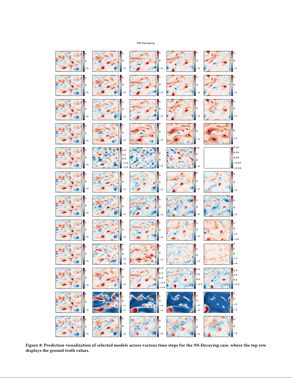
DSO: Dual-Scale Neural Operators for Long-term F luid Dynamics Forecasting Huanshuo Dong ∗ bingo000@mail.ustc.edu.cn University of Science and T echnology of China Hefei, China Hao W u ∗ T singhua University Beijing, China Hong W ang † wanghong1700@mail.ustc.edu.cn University of Science and T echnology of China Hefei, China Qin- Yi Zhang Institute of A utomation, Chinese Academy of Sciences Beijing, China Zhezheng Hao Zhejiang University Hangzhou, China Abstract Long-term uid dynamics forecasting is a critically important pr ob- lem in science and engineering. While neural operators have emerged as a promising paradigm for modeling systems governed by partial dierential equations (PDEs), they often struggle with long-term stability and precision. W e identify two fundamental failure modes in existing architectures: (1) local detail blurring, where ne-scale structures such as vortex cores and sharp gradients are progres- sively smoothed, and (2) global trend deviation, where the overall motion traje ctory drifts from the ground truth during extended rollouts. W e argue that these failures arise because existing neural operators treat local and global information processing uniformly , despite their inherently dierent evolution characteristics in physi- cal systems. T o bridge this gap, we propose the Dual-Scale Neural Operator (DSO), which explicitly decouples information processing into two complementary mo dules: depthwise separable convolu- tions for ne-grained local feature extraction and an MLP-Mixer for long-range global aggregation. Through numerical experiments on vortex dynamics, we demonstrate that nearby perturbations primarily aect local vortex structure while distant perturbations inuence global motion trends—providing empirical validation for our design choice. Extensive experiments on turbulent ow bench- marks show that DSO achieves state-of-the-art accuracy while maintaining robust long-term stability , reducing prediction error by over 88% compared to existing neural operators. A CM Reference Format: Huanshuo Dong, Hao Wu, Hong W ang, Qin- Yi Zhang, and Zhezheng Hao. 2018. DSO: Dual-Scale Neural Operators for Long-term F luid Dynamics Forecasting. In Proceedings of Make sure to enter the correct conference title ∗ Equal contribution. † Corresponding author . Permission to make digital or hard copies of all or part of this work for personal or classroom use is granted without fee provided that copies are not made or distributed for prot or commercial advantage and that copies bear this notice and the full citation on the rst page. Copyrights for components of this work owned by others than the author(s) must be honor ed. Abstracting with credit is permitted. T o copy otherwise, or republish, to post on servers or to redistribute to lists, requires prior specic permission and /or a fee. Request p ermissions from permissions@acm.org. Conference acronym ’XX, June 03–05, 2018, W oodstock, NY © 2018 Copyright held by the owner/author(s). Publication rights licensed to ACM. ACM ISBN 978-1-4503-XXXX -X/18/06 https://doi.org/XXXXXXX.XXXXXXX Ground T ruth DSO FNO LSM SimVP ConvLSTM 5.0 2.5 0.0 2.5 5.0 5.0 2.5 0.0 2.5 5.0 7.5 5.0 2.5 0.0 2.5 5.0 5.0 2.5 0.0 2.5 5.0 7.5 4 2 0 2 4 6 4 2 0 2 4 Visual Prediction Comparison (a) Visualization of long-term predictions for turbulence datasets from dierent models, where Ground Truth is the actual value and DSO is our method. 20 40 60 80 Time Step 10 4 10 3 10 2 10 1 10 0 10 1 Mean Squared Error (MSE) Prediction Errors over Times DSO FNO LSM SimVP ConvLSTM (b) Prediction errors of dierent models over time through autore- gressive rollout. The shaded areas repr esent the variance across dif- ferent samples. from your rights conrmation emai (Confer ence acronym ’XX). ACM, Ne w Y ork, N Y , USA, 13 pages. https://doi.org/XXXXXXX.XXXXXXX 1 Introduction Governed by partial dierential equations (PDEs), spatiotemporal dynamics prediction is a fundamental and critically important area Conference acronym ’XX, June 03–05, 2018, W oodstock, N Y Dong and Wu, et al. spanning physics, mathematics, and engineering disciplines [ 7 ]. Accurate long-term prediction of such dynamics is essential for scientic discovery and technological advancement, underpinning applications that range from weather forecasting and climate model- ing to computational uid dynamics [ 2 , 13 , 14 ]. In recent years, this eld has experience d a paradigm shift with the emergence of neural operators. These advanced deep learning architectures are explic- itly designed to learn the latent solution operator—the mapping between innite-dimensional function spaces for Partial Dieren- tial Equations (PDEs). Pione ering works, such as the Fourier Neural Operator (FNO) [ 9 ], the Convolutional Neural Operator (CNO) [ 18 ], and Latent Spectral Models (LSM) [ 23 ], have demonstrate d remarkable success in solving various PDEs, oering signicant computational speedups over traditional numerical solvers while maintaining reasonable accuracy for short-term predictions. Although neural operators have achie ved initial success in short- term prediction, applying them to long-term autoregressive fore- casting—where the model’s output at one time step b ecomes the input for the next—still faces signicant challenges. As sho wn in Figure 1b, existing methods exhibit a sharp increase in prediction error over extended time horizons. Figure 1a reveals two charac- teristic failure modes that compound over time . (1) Lo cal Detail Blurring : Fine-scale structures such as v ortex cores, sharp gradi- ents, and turbulent eddies are progressively smo othed out. This phenomenon, analogous to numerical diusion in classical solvers, results in loss of physically imp ortant small-scale features. Methods like FNO [ 9 ] produce increasingly blurred predictions, failing to preserve the sharp boundaries of coherent structures. (2) Global Trend Deviation : The ov erall motion trajectory—including vor- tex translation, rotation, and large-scale o w patterns—gradually drifts from the ground truth. This manifests as phase errors where predicted structures appear at wrong spatial locations, even when local features are reasonably preserved. For instance, SimVP [ 4 ] maintains local sharpness but exhibits signicant positional drift over extended rollouts. W e attribute these failures to a fundamental limitation: existing neural operators treat local and global information processing uni- formly , despite their inherently dierent characteristics in physical systems. In uid dynamics, nearby interactions directly ae ct lo- cal vortex structure thr ough mechanisms like vortex merging and strain-induced deformation, while distant interactions inuence global motion trends through pressur e-mediated coupling that acts across the entire domain. A single computational mechanism can- not optimally capture both eects. T o validate this hypothesis, we conduct numerical experiments with vorte x pairs at varying sep- arations (Section 4). Our results demonstrate a clear dichotomy: closely-spaced vortices exhibit strong local deformation with min- imal center displacement, while widely-separate d vortices show little lo cal interaction but signicant trajectory dee ction. This empirical evidence motivates e xplicit separation of local and global processing pathways. T o overcome this critical limitation, we propose the Dual-Scale Neural Operator (DSO) , which introduces a physics-motivated dual-pathway mechanism for spatiotemporal data processing. Our architecture integrates two synergistic components: (1) a Local Processing Module via Depthwise Separable Convolution that captures ne-scale features, gradient structur es, and local interac- tions within a bounded receptive eld, responsible for preserving local details and preventing numerical diusion; and (2) a Global Processing Module via MLP-Mixer that aggregates information across the entire spatial domain through channel-wise and spatial mixing operations, capturing long-range dependencies and main- taining corr ect global motion trends. By explicitly decoupling these two processing pathways, DSO simultaneously pre vents local detail blurring and global trend deviation—addressing both failure modes of existing approaches. Extensive validation on canonical turbulent ow benchmarks un- equivocally demonstrates the superior performance and robust sta- bility of DSO in long-term spatiotemporal forecasting. Our metho d achieves substantial improvement in prediction accuracy , reducing prediction error by over 88% compar ed to existing state-of-the-art methods. Crucially , DSO maintains robust stability over extended prediction horizons where conventional methods quickly fail. This stability stems from the dual-pathway mechanism’s ability to eec- tively address both local diusion and global drift simultaneously . Our main contributions are: • W e identify and analyze two fundamental failure modes in long- term neural operator predictions: local detail blurring and global trend deviation. • Through numerical experiments on vortex dynamics, we demon- strate that local and global perturbations have qualitatively dier- ent eects, providing physical motivation for separate processing mechanisms. • W e propose DSO, a dual-scale neural operator that explicitly decouples local and global information processing through con- volution and MLP-Mixer modules. • Extensive experiments demonstrate that DSO achiev es state-of- the-art accuracy while maintaining long-term stability across multiple challenging benchmarks. 2 Related W ork 2.1 T urbulence prediction T urbulence prediction remains a challenging problem due to the complex, chaotic nature of uid ows governed by the Navier- Stokes (NS) equations [ 8 ]. Traditional numerical methods, such as direct numerical simulation and large eddy simulation, provide accurate solutions but suer from high computational costs, par- ticularly for long-term predictions [ 16 ]. Data-driven approaches, such as deep learning-based models, have emerged as promising al- ternatives, oering potential for real-time for ecasting with reduced computational overhead. Early works like [ 20 ] applied neural net- works to predict turbulent dynamics, but these models struggled with generalizing to unseen ow regimes. Recent advancements have incorporated physical constraints, like the NS equations, into neural network training, ensuring better adherence to the govern- ing laws of uid dynamics [ 6 , 22 ]. Despite these improvements, long-term prediction of turbulence still faces issues like loss of ne-scale features and failure to pr eserve physical consistency in extended forecasts [ 1 ]. These challenges highlight the need for more sophisticated models that can integrate spatial and temporal adaptivity , as well as global physical consistency . DSO: Dual-Scale Neural Operators for Long-term Fluid Dynamics Forecasting Conference acronym ’XX, June 03–05, 2018, W oodstock, N Y 2.2 Neural op erator and vide o prediction model Neural operators have be come central to solving complex PDEs by directly learning mappings between input and output data. Fourier Neural Operator (FNO) [ 9 ] leverages the Fast Fourier Transform to eciently approximate solutions in the spectral domain, balancing accuracy with computational eciency . Further extensions, such as U-NO [ 17 ] and CNO [ 18 ], enhance the model’s ability to han- dle multi-scale dynamics. LSM [ 23 ] addresses high-dimensional PDEs by incorporating spectral methods in learned latent spaces. Models such as ConvLSTM [ 10 ], ResNet [ 5 ], and PastNet [ 24 ] excel in capturing temporal dependencies, making them well-suited for dynamic forecasting tasks like turbulence prediction. The integra- tion of attention mechanisms in models like Swin T ransformer [ 11 ] and SimVP [ 4 ] further enhances their ability to model long-range temporal dynamics. These models oer promising avenues for ad- vancing turbulence prediction, where both spatial and temporal complexities must be captured simultaneously . 3 Preliminary 3.1 Problem Denition W e consider the two-dimensional (2D) Navier-Stokes equations for a viscous, incompressible uid [ 3 , 9 , 21 ]. The dynamics are expressed in vorticity form on the unit torus T 2 = [ 0 , 2 𝜋 ] 2 with periodic boundar y conditions. The evolution of the scalar vorticity eld, 𝝎 ( 𝑥 , 𝑡 ) , is governed by: 𝜕 𝑡 𝝎 + ( u · ∇) 𝝎 = 𝜈 Δ 𝝎 + 𝑓 , ( 𝑥 , 𝑡 ) ∈ T 2 × ( 0 , 𝑇 ] , (1) 𝝎 ( 𝑥 , 0 ) = 𝝎 0 ( 𝑥 ) , 𝑥 ∈ T 2 . (2) Here, 𝝎 is the vorticity , u is the div ergence-free velocity eld, 𝜈 > 0 is the kinematic viscosity , and 𝑓 is a time-indep endent external forcing. The velocity eld u is recovered fr om the vorticity 𝝎 via the Biot-Savart law , which is dene d through the stream-function 𝜓 : u = ∇ ⊥ 𝜓 = ( 𝜕 𝑥 2 𝜓 , − 𝜕 𝑥 1 𝜓 ) , − Δ 𝜓 = 𝝎 . (3) This relationship closes the system, rendering the advection term ( u · ∇) 𝝎 a non-local quadratic nonlinearity in 𝝎 . For suitable initial conditions 𝝎 0 and forcing 𝑓 (e.g., in 𝐿 2 ( T 2 ) ), the system is glob- ally well-posed, guaranteeing a unique solution trajectory whose regularity depends on the smoothness of the initial data [3]. Our obje ctive is to learn a parameterized op erator , G 𝜃 , that ap- proximates the true solution operator , G [ 9 ]. This operator maps a history of the vorticity eld ov er an input interval [ 0 , 𝑇 𝑖𝑛 ] to its future evolution o ver a subsequent interval ( 𝑇 𝑖𝑛 , 𝑇 ] . Formally , the mapping is: G : 𝐶 ( [ 0 , 𝑇 𝑖𝑛 ] ; 𝐻 𝑟 ( T 2 ) ) → 𝐶 ( ( 𝑇 𝑖𝑛 , 𝑇 ] ; 𝐻 𝑟 ( T 2 ) ) , (4) where 𝐻 𝑟 ( T 2 ) is the Sobolev space of order 𝑟 , chosen to reect the regularity of the data in our experiments. In practice, our model learns a one-step mapping that is applied autoregressively to per- form this long-horizon forecasting, eectively propagating the so- lution in time. 3.2 A utoregr essive Rollout The learned operator G 𝜃 is trained to predict a single future state from a sequence of past observations. Specically , given a history of 𝑇 𝑖𝑛 consecutive vorticity elds { 𝝎 ( 𝑡 − 𝑇 𝑖𝑛 + 1 ) , . . . , 𝝎 ( 𝑡 ) } , the model predicts the next state: ˆ 𝝎 ( 𝑡 + 1 ) = G 𝜃 ( 𝝎 ( 𝑡 − 𝑇 𝑖𝑛 + 1 ) , . . . , 𝝎 ( 𝑡 ) ) . (5) For long-term prediction over 𝑇 𝑝𝑟 𝑒 𝑑 steps, we apply the mo del autoregressively . The predicte d state ˆ 𝝎 ( 𝑡 + 1 ) is appended to the input sequence, and the oldest frame is discarded: ˆ 𝝎 ( 𝑡 + 𝑘 + 1 ) = G 𝜃 ( ˆ 𝝎 ( 𝑡 + 𝑘 − 𝑇 𝑖𝑛 + 1 ) , . . . , ˆ 𝝎 ( 𝑡 + 𝑘 ) ) , 𝑘 = 1 , 2 , . . . , 𝑇 𝑝𝑟 𝑒 𝑑 − 1 . (6) Note that after the initial prediction, all subsequent inputs con- sist entirely of model-generated states, making the model highly susceptible to error accumulation. Any prediction error at step 𝑘 propagates to all future steps, potentially leading to divergence from the true trajectory . This error compounding phenomenon is the central challenge addressed in this work. 4 Motivation W e observe that local and global perturbations have fundamentally dierent eects on vortex dynamics, indicating that a single-scale mechanism cannot optimally capture both ne-scale structural changes and large-scale trajector y evolution. This observation mo- tivates our dual-scale algorithm design. 4.1 Experimental Setup W e simulate 2D incompressible Navier-Stokes ow using a pseudo- spectral method on a 128 × 128 perio dic domain [ 0 , 2 𝜋 ] 2 (details in Appendix A.1). W e compare two scenarios: a vortex dipole with a perturbing vortex placed at close distance ( 𝑑 = 0 . 6 ) vs. far distance ( 𝑑 = 2 . 5 ), isolating local and global eects respectively . 4.2 Ke y Obser vations Figure 2 shows the temp oral evolution of b oth scenarios. W e observe strikingly dierent behaviors: Close Perturbation (Local Eect): The nearby vortex induces strong lo cal deformation of the dipole structure . The vortices stretch, merge partially , and exhibit complex ne-scale interactions. This leads to signicant gradient intensication within the local region. Although the system also exhibits global displacement, the domi- nant eect is the enhancement of ne-scale structure complexity . Far Perturbation (Global Eect): The distant v ortex barely aects the dipole’s internal structure. Without nearby disturbance, the local gradients gradually weaken over time. Instead, the far vorte x changes the dipole’s moving direction thr ough long-range pressure eects, while leaving its internal shape unchanged. 4.3 Quantitative Analysis T o quantify these obser vations, we track two metrics: • Local Deformation : Maximum vorticity gradient max ( ∥ ∇ 𝜔 ∥ ) . The vorticity gradient measures how rapidly the rotation inten- sity changes across space. Its increase indicates the formation of ne-scale structures (e .g., sharp vortex edges), while its decrease reects structural smoothing. • Global Displacement : Center-of-vorticity position x 𝑐 = ∫ x | 𝜔 | 𝑑 x  ∫ | 𝜔 | 𝑑 x . Conference acronym ’XX, June 03–05, 2018, W oodstock, N Y Dong and Wu, et al. Close V ortices (V orticity ) F ar V ortices (V orticity ) Figure 2: T emporal evolution of vortex dipole under close (top) vs. far (bottom) p erturbations. The curve represents a streamline of the ow eld. The red-blue vortex pair on the left represents the dipole, while the isolate d vortex on the right is the perturbing vortex. T able 1: Comparison of ee cts for p erturbations. Metric Close ( 𝑑 = 0 . 6 ) Far ( 𝑑 = 2 . 5 ) Local gradient change Δ max ( ∥ ∇ 𝜔 ∥ ) +45% − 29% Global position shift ∥ Δ x 𝑐 ∥ 0.8 0.6 T able 1 summarizes the results. The key distinction lies in the nature of the eect rather than its magnitude. The close perturba- tion causes a 45% increase in local gradient intensity due to vortex stretching and ne-scale interactions—the nearby vorte x actively enhances structural complexity . In contrast, the far perturbation leads to gradient decay ( − 29%) as the dipole evolves undisturbed by local interference; the isolated dipole simply dissipates gradually . While both scenarios show similar global displacement magnitudes (0.8 vs 0.6), the underlying mechanisms are fundamentally dierent: close perturbations create local structural changes, while far per- turbations inuence dynamics through non-local pressure coupling without aecting local structure. This experiment reveals a fundamental dichotomy in uid dynam- ics: • Local interactions (nearby vortices) primarily aect ne-scale structure within a bounde d spatial region. • Global interactions (distant vortices) primarily aect motion trajectory through domain-wide pressure coupling. 5 Method Based on our observation that local and global information propa- gation have fundamentally dierent eects in uid dynamics (Sec- tion 4), w e propose the Dual-Scale Operator (DSO ) . DSO explicitly separates local and global processing through two complementary pathways: conv olutions for local feature extraction and MLP-Mixer for global information aggregation. 5.1 Overall Architecture As shown in Figure 3, DSO implements the prediction mapping through: ˆ 𝝎 ( 𝑡 + 1 ) = D ◦ T ◦ E ( 𝝎 ( 𝑡 ) ) , (7) where E , T , and D represent the enco der , dual-scale translator , and decoder , respectively . The input is a sequence of vorticity elds 𝝎 in ∈ R 𝐵 × 𝑇 × 𝐶 × 𝐻 × 𝑊 (batch, time, channel, height, width). The out- put is the predicted next state ˆ 𝝎 ∈ R 𝐵 × 𝑇 × 𝐶 × 𝐻 × 𝑊 . 5.2 Encoder-Decoder Encoder . The encoder E progressively reduces spatial resolution while increasing feature channels through 𝑁 𝑠 convolutional layers: 𝑝 𝑖 = 𝜎 ( Norm ( Conv ( 𝑝 𝑖 − 1 ) ) ) , 1 ≤ 𝑖 ≤ 𝑁 𝑠 , (8) where 𝑝 0 = 𝝎 ( 𝑡 ) is the input vorticity eld, 𝑁 𝑠 is the number of encoder layers, and 𝜎 is a nonlinear activation. The shallow-layer features 𝑝 1 are preserved for skip connections. Decoder . The de coder D reconstructs the output through 𝑁 𝑠 trans- posed convolutional layers: 𝑞 𝑖 = 𝜎 ( Norm ( ConvT ( 𝑞 𝑖 − 1 ) ) ) , 1 ≤ 𝑖 ≤ 𝑁 𝑠 − 1 , (9) where 𝑞 0 = ˜ 𝑧 is the translator output. The nal layer incorporates skip connections from the encoder: ˆ 𝝎 ( 𝑡 + 1 ) = Proj ( 𝜎 ( Norm ( ConvT ( [ 𝑞 𝑁 𝑠 − 1 , 𝑝 1 ] ) ) ) ) , (10) where [ · , ·] denotes concatenation and Proj is a 1 × 1 convolution that projects to output channels. 5.3 Dual-Scale Translator The translator T is the core of DSO, consisting of 𝑁 𝑡 stacked dual- pathway blocks. Each block sequentially applies lo cal and global processing: 𝑧 ′ = F local ( 𝑧 𝑘 ) , 𝑧 𝑘 + 1 = F global ( 𝑧 ′ ) . (11) DSO: Dual-Scale Neural Operators for Long-term Fluid Dynamics Forecasting Conference acronym ’XX, June 03–05, 2018, W oodstock, N Y z i+ 1 Dua l- Sca le T ra ns la t o r … M ixB loc k 1 M ixB loc k N t M ixB loc k 2 M ix B lo ck T C on v olu ti o n z i M LP - M ixe r c o nv c o nv … … M LP E nco der Deco der   �   +  vo r t ex vo r t ex Figure 3: Over view of DSO architecture. The model consists of three components: (1) an encoder E that extracts multi-scale spatial features, (2) a translator T composed of stacked dual-pathway blocks, and (3) a deco der D that reconstructs the predicted eld. Each block contains a Lo cal Pathway (convolution) for ne-scale features and a Global Pathway (MLP-Mixer) for domain- wide information aggregation. The cur ved arrows connecting the encoder and de coder represent skip connections. Design rationale: Base d on the observation in Section 4, we use convolution for local processing (bounded receptive eld captur es ne-scale vortex structures) and MLP-Mixer for global processing (all-to-all spatial communication models domain-wide pressure coupling). The sequential order—local before global—ensures that ne-scale features are rst extracted, then aggregated into coherent global patterns. 5.3.1 Local Pathway: Convolution . W e employ depthwise sepa- rable convolutions: F local ( 𝑧 ) = 𝑧 + 𝛾 · Conv point ( 𝜎 ( Conv depth ( Norm ( 𝑧 ) ) ) ) , (12) where Conv depth is a depthwise convolution, Conv point is a point- wise convolution for channel mixing, and 𝛾 is a learnable scaling parameter . 5.3.2 Global Pathway: MLP-Mixer . W e employ spatial and chan- nel mixing: F global ( 𝑧 ) = 𝑧 + MLP channel ( Norm ( MLP spatial ( Norm ( 𝑧 ) ) ) ) , (13) where MLP spatial operates across all spatial locations for each chan- nel, and MLP channel mixes feature representations across channels. 6 Experiment 6.1 Experiment Setting Implementation Details. All models in this paper are trained on a server equipp ed with eight N VIDIA A100 GP Us (40GB memory per card). W e employ the DistributedDataParallel mode from the Py T orch framework [ 15 ] for distributed training to accelerate con- vergence. Model inference is conducted on a single NVIDIA A100 GP U. The experimental software environment is built on Python 3.8, with Py T orch 1.8.1 (CUD A 11.1) and T orchVision 0.9.1. Throughout training, we maintain a consistent hyperparameter conguration: batch size of 20, total epochs of 500, and an initial learning rate of 0.001. T o ensure experimental reproducibility , all random seeds are xed to 42. For training, the model adopts one-step prediction, i.e., using one time step to predict the next. During testing, a rollout approach is used: the rst time step predicted the next, and the result was fed as input for subsequent predictions, iterating this cycle to forecast multiple time steps. Further experimental details are provided in the Appendix A.2.1. Datasets. W e evaluate various models on two representative uid dynamics datasets, aiming to assess their ability to capture long- term uid motion under dierent physical conditions. • NS-Forced (Navier-Stokes Forced T urbulence) Benchmark : This dataset is based on the Navier-Stokes benchmark proposed by [ 9 ]. The kinematic viscosity is set to 𝜈 = 10 − 5 . The initial vorticity eld 𝜔 0 is sample d from a zero-mean Gaussian random eld with a covariance operator ( − Δ + 𝜏 2 𝐼 ) − 𝛼 / 2 , where Δ is the Laplacian operator , 𝐼 is the identity operator , and 𝜏 and 𝛼 are parameters controlling the shape of the energy spectrum. The energy density 𝐸 ( 𝑘 ) follows the decay law 𝐸 ( 𝑘 ) ∼ ( 𝑘 2 + 𝜏 2 ) − 𝛼 . The ow is continuously driven by a xed external force at low wavenumbers, with no additional drag eects introduced. • NS-Decaying (Navier-Stokes Decaying Turbulence) : This dataset simulates the natural decay of turbulence [ 12 ]. The power spectrum of the initial stream function is dened by ˆ 𝜓 ( 𝑘 ) 2 ∼ 𝑘 − 1 ( 𝜏 2 0 + ( 𝑘 / 𝑘 0 ) 4 ) − 1 , where 𝑘 0 is the characteristic wavenumber and 𝜏 0 is a spectral shape parameter; this expres- sion determines the structure of the initial ow eld. This ini- tial condition is specically designe d to achieve slow energy dissipation, and the evolution of vorticity density over time Conference acronym ’XX, June 03–05, 2018, W oodstock, N Y Dong and Wu, et al. T able 2: MSE comparison across methods for NS-Forced and NS-De caying turbulence. “All-step ” denotes the average error over all prediction steps, while “ 𝑖 -step” indicates the error at the 𝑖 -th sp ecic prediction step. Lower MSE values indicate better performance, while "nan" indicates excessive model error or data overow , suggesting model collapse. Method NS-Forced NS-Decaying All-step 1-step 10-step 19-step All-step 1-step 50-step 99-step DSO 0.0153 0.0001 0.0015 0.1086 0.1714 0.0003 0.1271 0.4986 UNO 0.2752 0.0037 0.0974 1.1894 nan 0.1771 nan nan CNO 0.3790 0.0008 0.1116 1.6521 4.5553 0.0390 5.2277 6.2792 FNO 0.0263 0.0001 0.0024 0.1852 1.6333 0.0242 1.7299 2.9465 U_Net 0.1278 0.0007 0.0308 0.6620 2.9288 0.0177 3.3029 4.6783 LSM 0.0779 0.0002 0.0086 0.4988 2.8647 0.0033 3.1483 5.2504 Swin 0.1268 0.0002 0.0271 0.6362 3.2328 0.0070 3.7928 5.0429 ConvLSTM 1.3521 0.0101 1.2379 3.1692 3.3228 0.1078 3.7786 3.1913 SimVP 0.0718 0.0003 0.0115 0.4290 1.5510 0.0016 1.5575 3.2480 ResNet 0.5906 0.0023 0.2180 2.1835 4.7140 0.0674 5.3391 6.6097 PastNet 0.1349 0.0012 0.0326 0.6009 3.2089 0.1879 3.6807 5.1670 exhibits characteristics resembling the K olmogorov energy cas- cade. This turbulence is force-free and evolves entirely from the initial conditions. More details can be found in the Appendix A.2.2. Baseline. W e evaluate our method against leading models from neural operators, computer vision, and time series prediction. For neural operators, we select FNO [ 9 ], UNO [ 17 ], CNO [ 18 ], and LSM [ 23 ] as representative architectures for learning PDE solution map- pings. In computer vision, we adopt ResNet [ 5 ], U-net [ 19 ], and Swin Transformer [ 11 ] due to their strong spatial feature extrac- tion capabilities. For time series prediction, we employ ConvLSTM [ 10 ], PastNet [ 24 ], and SimVP [ 4 ], which excel in capturing tempo- ral dynamics. The model sizes and congurations are detaile d in Appendix A.2.3. 6.2 Main Results T able 2 provides a compr ehensive comparison of the Mean Squared Error (MSE) performance for various methods across two scenarios: NS-Forced and NS-De caying turbulence . Meanwhile, Figure 6 show- cases the prediction results for a subset of these methods, with the visualizations for the remaining methods detailed in the Appendix A.2.4. Our DSO approach demonstrates superior performance and marked long-term stability , which is substantiated by the following key observations: Consistent State-of-the-Art Performance : DSO achieves the lowest err or across nearly all e valuation metrics in both datasets. For NS-Forced, DSO reduces the all-step error to just 58.2% of the second-best method’s performance (0.0153 vs. FNO’s 0.0263). In the more challenging NS-Decaying scenario, DSO achiev es an e ven more dramatic improvement, r educing the all-step error to merely 11.0% of the ne xt best performer’s result (0.1714 vs. SimVP ’s 1.5510), which means our method reduces the prediction error by over 88%. Exceptional Long-T erm Stability : DSO demonstrates remarkable robustness in extended temporal predictions, maintaining physical consistency where competing methods catastrophically fail. In NS- Forced at the critical 19-step horizon (near simulation limits), DSO sustains a remarkably low error of 0.1086—reducing the error to merely 58.6% of FNO’s performance (0.1852), 9.1% of UNO’s (1.1894), 6.6% of CNO’s (1.6521), and 5.0% of ResNet’s (2.1835). The stability advantage becomes even more pronounced in NS-Decaying at the extreme 99-step horizon. While most methods suer numerical col- lapse (UNO produces NaN values across all long-horizon metrics), DSO achieves an err or of 0.4986—reducing the error to just 16.9% of FNO’s result (2.9465), 15.4% of SimVP’s (3.2480). Visualization Analysis : Figure 6 presents the experimental re- sults of selected methods on the NS-De caying dataset. The visu- alization reveals sev eral limitations in baseline approaches: the best-performing baseline method FNO exhibits blurred turbulent details; ConvLSTM suers from numerical collapse during long- term predictions; While LSM maintains detailed ow structures, it demonstrates signicant motion drift over extended horizons. For instance, LSM’s pr ediction incorrectly splits the vortex in the central-lower region into two structures. In contrast, our method successfully avoids all these issues. Even at the 99th time step, our predictions remain visually nearly identical to the ground truth. This stable error propagation—devoid of numerical instabilities even at the maximum prediction horizon—validates the core innovation of DSO: its dual-scale architecture explicitly separates lo cal and global processing to match the fundamental dichotomy in uid dy- namics. As demonstrated in our motivation e xperiments (Section 4), local information primarily governs ne-scale vortex structure and gradient dynamics, while global information controls motion tra- jectories through domain-wide pressur e coupling. By employing depthwise separable convolutions for local feature extraction ( cap- turing gradient intensication and vortex deformation) and MLP- Mixer for global information aggregation (modeling long-range spatial dependencies), DSO simultaneously preser ves ne-grained turbulent details in regions with steep gradients while maintaining coherent large-scale motion predictions. This physics-informed dual-scale design meets the critical requirements for reliable uid DSO: Dual-Scale Neural Operators for Long-term Fluid Dynamics Forecasting Conference acronym ’XX, June 03–05, 2018, W oodstock, N Y 20 40 60 80 Time Step 0.0 0.2 0.4 0.6 0.8 1.0 S SIM S SIM Performance Comparison Over Time DSO CNO FNO LSM ConvLSTM SimVP Figure 4: W e selected predictions from selected models on the NS-Decaying dataset, computed and analyzed the mean and variance of their SSIM values. prediction in scientic and engineering applications—esp ecially in scenarios requiring accurate long-horizon forecasting where single- scale approaches fail to capture the multi-scale nature of turbulent ows. 6.3 Analytical Exp eriment 6.3.1 SSIM Evaluation Metrics. In uid dynamics forecasting, rely- ing solely on Mean Squared Error (MSE) is limited. MSE measures only pixel-level numerical discrepancies and fails to distinguish between critical physical structure errors (like vortex displacement) and minor numerical uctuations. Giv en that turbulence prediction prioritizes the preservation of critical physical features such as vor- tex morphology , we complement our analysis with the Structural Similarity Index (SSIM) (details pr ovided in the Appendix A.2.5). Our experimental results show that DSO maintains signicant su- periority in SSIM metrics, particularly ensuring stable forecasting reliability during long-term predictions. W e also note that while certain baselines (SimVP, LSM, FNO) sho w acceptable MSE perfor- mance mid-term ( ∼ 50 time steps), their structural preservation varies. For instance, LSM and ConvLSTM may exhibit similar MSE at 50 steps, but Figure 4 clearly sho ws LSM’s superior ability to pre- serve discernible vortex features. This comparison underscores the critical importance of evaluating both quantitative metrics (MSE) and structural delity (SSIM) in assessing turbulence forecasting performance. 6.3.2 Gradient and Divergence Evaluation Metrics. Gradient ∇ u =  𝜕𝑢 𝜕𝑥 , 𝜕𝑢 𝜕 𝑦  and divergence ∇ · u = 𝜕𝑢 𝜕𝑥 + 𝜕 𝑣 𝜕 𝑦 analysis validates physi- cal delity of predictions. Gradient elds capture critical deforma- tion features—strain rates, vortex stretching, and coherent struc- tures—that govern turbulent energy transfer . Divergence elds verify mass conservation, where non-zero values reveal unphysical instabilities. T ogether , they ensure predictions maintain both struc- tural accuracy and fundamental physical constraints, essential for trustworthy scientic applications. Experimental results demonstrate that DSO achieves signicantly lower prediction err ors than competing methods, demonstrating exceptional capability in capturing ow dynamics and maintaining dynamic consistency across all prediction horizons. 6.4 Ablations T o analyze the contribution of individual modules in our dual-scale architecture, w e conduct ablation studies by separately removing the convolution module (local processing) and the MLP-Mixer mod- ule (global processing) from the MixBlock, while keeping all other hyperparameters and settings identical to the main experiments. Specically , “w/o Conv” removes the depthwise separable convolu- tion branch, and “w/o MLP-Mixer” remov es the MLP-Mixer branch. T able 3: Ablation study of DSO on the NS-Decaying dataset Method All-step 1-step 50-step 99-step DSO 0.1714 0.0003 0.1271 0.4986 w/o Conv 0.2059 0.0004 0.1565 0.5871 w/o MLP-Mixer 1.1335 0.0010 1.1330 2.4606 The results re veal distinct roles for each module in our dual-scale design. Removing the MLP-Mixer module causes the most signi- cant performance degradation (All-step err or increases from 0.1714 to 1.1335, a 6.6 × increase), conrming that global processing is es- sential for capturing long-range spatial dependencies and maintain- ing prediction stability . At the 99-step horizon, the error increases nearly 5 × (from 0.4986 to 2.4606), demonstrating that without global information aggregation, the model fails to accurately predict large- scale motion trajectories. Removing the convolution module also degrades performance (All-step error increases to 0.2059), indicating that local processing contributes to capturing ne-scale turbulent structures. These results validate our dual-scale design: both local and global processing are indispensable, with global processing playing a particularly critical role in long-term prediction stability . 7 Conclusion W e propose DSO (Dual-scale Spatiotemporal Op erator), a neural operator that combines local convolutions and global MLP-Mixer to capture multi-scale ow dynamics. Experiments on for ced and decaying turbulence benchmarks demonstrate that DSO addresses key limitations of existing methods—blurred details, trend bias, and numerical collapse—achieving up to 89% error reduction while maintaining stability at extreme time horizons. These results es- tablish DSO as a robust solution for long-horizon uid dynamics prediction. 8 Limitations and Ethical Considerations While our method shows pr omising results, future work may ex- plore e xtensions to br oader physical scenarios and boundary condi- tions. This work focuses on scientic computing for uid dynamics, posing minimal ethical risks. W e encourage responsible use and proper validation in downstream applications. Conference acronym ’XX, June 03–05, 2018, W oodstock, N Y Dong and Wu, et al. 20 40 60 80 Time Step 0 1 2 3 4 5 6 Gradient V ector Error Norm DSO CNO FNO LSM ConvLSTM SimVP (a) Gradient V ector error comparison over time 20 40 60 80 Time Step 0.0 0.5 1.0 1.5 2.0 Divergence Error DSO CNO FNO LSM ConvLSTM SimVP (b) Divergence error comparison over time Figure 5: Comparison of gradient and divergence errors of dierent methods on the NS-Decaying dataset. (a) Gradient magnitude error quanties the accuracy of capturing ow deformation features. (b) Divergence error measures physical consistency and mass conservation properties. Ground T ruth T ime Step 1 T ime Step 30 T ime Step 60 T ime Step 80 T ime Step 99 DSO FNO LSM ConvLSTM 5 0 5 5 0 5 5 0 5 5 0 5 5 0 5 5 0 5 5 0 5 5 0 5 5 0 5 5 0 5 5 0 5 5 0 5 5 0 5 5 0 5 5 0 5 5 0 5 5 0 5 5 0 5 5 0 5 5 0 5 5 0 5 4 2 0 2 4 2 0 2 2 0 2 4 2 0 2 4 Comparison of All Methods at Different Time Steps Figure 6: Prediction visualization of sele cted models across various time steps for the NS-Decaying case, where the top row displays the ground truth values. DSO: Dual-Scale Neural Operators for Long-term Fluid Dynamics Forecasting Conference acronym ’XX, June 03–05, 2018, W oodstock, N Y References [1] Haoming Cai, Jingxi Chen, Brandon Feng, W eiyun Jiang, Mingyang Xie, Kevin Zhang, Cornelia Fermuller , Yiannis Aloimonos, Ashok V eeraraghavan, and Chris Metzler . 2024. T emporally consistent atmospheric turbulence mitigation with neural representations. Advances in Neural Information Processing Systems 37 (2024), 44554–44574. [2] Karthik Duraisamy , Gianluca Iaccarino, and Heng Xiao. 2019. T urbulence model- ing in the age of data. A nnual review of uid me chanics 51, 1 (2019), 357–377. [3] Lawrence C Evans. 2022. Partial dierential equations . V ol. 19. American mathe- matical society . [4] Zhangyang Gao, Cheng T an, Lirong Wu, and Stan Z Li. 2022. Simvp: Simpler yet better video prediction. In Procee dings of the IEEE/CVF conference on computer vision and pattern recognition . 3170–3180. [5] Kaiming He, Xiangyu Zhang, Shaoqing Ren, and Jian Sun. 2016. Deep residual learning for image recognition. In Procee dings of the IEEE conference on computer vision and pattern recognition . 770–778. [6] Vijay Kag, Kannabiran Seshasayanan, and V enkatesh Gopinath. 2022. Physics- informed data based neural networks for two-dimensional turbulence. P hysics of Fluids 34, 5 (2022). [7] Nikola B Kovachki, Samuel Lanthaler , and Andrew M Stuart. 2024. Operator learning: Algorithms and analysis. Handb ook of Numerical A nalysis 25 (2024), 419–467. [8] Lev Davido vich Landau and Evgeny Mikhailovich Lifshitz. 1987. Fluid Me chanics: V olume 6 . V ol. 6. Elsevier . [9] Zongyi Li, Nikola Borislavov K ovachki, Kamyar Azizzadenesheli, Burigede liu, Kaushik Bhattacharya, Andrew Stuart, and Anima Anandkumar . 2021. Fourier Neural Operator for Parametric Partial Dierential Equations. In International Conference on Learning Representations . [10] Zhihui Lin, Maomao Li, Zhuobin Zheng, Y angyang Cheng, and Chun Yuan. 2020. Self-attention convlstm for spatiotemporal pr ediction. In Proceedings of the AAAI conference on articial intelligence , V ol. 34. 11531–11538. [11] Ze Liu, Y utong Lin, Y ue Cao, Han Hu, Yixuan W ei, Zheng Zhang, Stephen Lin, and Baining Guo. 2021. Swin transformer: Hierarchical vision transformer us- ing shifted windows. In Proceedings of the IEEE/CVF international conference on computer vision . 10012–10022. [12] James C McWilliams. 1984. The emergence of isolated coherent vortices in turbulent ow . Journal of F luid Me chanics 146 (1984), 21–43. [13] T omás Norton and Da- W en Sun. 2006. Computational uid dynamics (CFD)–an eective and ecient design and analysis tool for the food industry: a review . Trends in Fo od Science & Technology 17, 11 (2006), 600–620. [14] Tim N Palmer. 2019. Stochastic weather and climate models. Nature Reviews Physics 1, 7 (2019), 463–471. [15] Adam Paszke, Sam Gross, Francisco Massa, Adam Lerer , James Bradbury, Gregory Chanan, T revor Killeen, Zeming Lin, Natalia Gimelshein, Luca Antiga, et al . 2019. Pytorch: An imperative style, high-performance deep learning library. Advances in neural information processing systems 32 (2019). [16] Stephen B Pope. 2001. Turbulent o ws. Measurement Science and Technology 12, 11 (2001), 2020–2021. [17] Md Ashiqur Rahman, Zachary E Ross, and Kamyar Azizzadenesheli. 2022. U-no: U-shaped neural operators. arXiv preprint arXiv:2204.11127 (2022). [18] Bogdan Raonic, Roberto Molinaro, T obias Rohner , Siddhartha Mishra, and Em- manuel de Bezenac. 2023. Convolutional neural op erators. In ICLR 2023 workshop on physics for machine learning . [19] Olaf Ronneberger , Philipp Fischer , and Thomas Brox. 2015. U-net: Convolutional networks for biomedical image segmentation. In International Conference on Medical image computing and computer-assisted intervention . Springer , 234–241. [20] Prem A Srinivasan, L Guastoni, Hossein Azizpour , PHILIPP Schlatter , and Ricardo Vinuesa. 2019. Predictions of turbulent shear ows using deep neural networks. Physical Review Fluids 4, 5 (2019), 054603. [21] Makoto T akamoto, Timothy Praditia, Raphael Leiteritz, Daniel MacKinlay , Francesco Alesiani, Dirk Püger, and Mathias Niepert. 2022. Pdebench: An extensive benchmark for scientic machine learning. Advances in Neural Infor- mation Processing Systems 35 (2022), 1596–1611. [22] Rui Wang, Karthik Kashinath, Mustafa Mustafa, Adrian Alb ert, and Rose Yu. 2020. T owards physics-informed deep learning for turbulent ow prediction. In Proceedings of the 26th A CM SIGKDD international conference on knowledge discovery & data mining . 1457–1466. [23] Haixu Wu, T engge Hu, Huakun Luo, Jianmin W ang, and Mingsheng Long. 2023. Solving High-Dimensional PDEs with Latent Spectral Models. In Proceedings of the 40th International Conference on Machine Learning . 37417–37438. [24] Hao Wu, Fan Xu, Chong Chen, Xian-Sheng Hua, Xiao Luo, and Haixin W ang. 2024. Pastnet: Introducing physical inductive biases for spatio-temporal video prediction. In Proceedings of the 32nd ACM international conference on multimedia . 2917–2926. A Appendix A.1 Motivation Exp eriment Details A.1.1 Governing Equations and Numerical Method. W e simulate 2D incompressible ow gov erned by the vorticity-streamfunction formulation of the Navier-Stokes equations: 𝜕𝜔 𝜕𝑡 + ( u · ∇) 𝜔 = 𝜈 ∇ 2 𝜔 , ∇ 2 𝜓 = − 𝜔 (14) where 𝜔 is the vorticity , 𝜓 is the streamfunction, u = ( 𝜕 𝑦 𝜓 , − 𝜕 𝑥 𝜓 ) is the velocity , and 𝜈 is the viscosity . W e use a pseudo-spectral method with 4th-order Runge-Kutta time integration on a 128 × 128 periodic domain. A.1.2 Experimental Configuration. W e construct two scenarios to isolate local and global eects: • Scenario A (Close Perturbation) : A vortex dipole (counter- rotating pair) with a single perturbing vorte x placed at distance 𝑑 𝑐𝑙 𝑜 𝑠 𝑒 = 0 . 6 from the dipole center . • Scenario B (Far Perturbation) : The same dipole conguration with the perturbing vortex placed at distance 𝑑 𝑓 𝑎𝑟 = 2 . 5 . The dipole is identical in both cases, allowing direct comparison of how perturbation distance aects the dynamics. A.1.3 antitative Metrics. T o quantify the observations, we track two metrics: • Local Deformation : Maximum vorticity gradient ∥ ∇ 𝜔 ∥ max within a local region centered at the vortex center , measuring ne-scale structure intensity . • Global Displacement : Center-of-vorticity position x 𝑐 = ∫ x | 𝜔 | 𝑑 x / ∫ | 𝜔 | 𝑑 x . T able 4 summarizes the results: T able 4: Comparison of local and global eects for close vs. far perturbations. Metric Close ( 𝑑 = 0 . 6 ) Far ( 𝑑 = 2 . 5 ) Local gradient change Δ ∥ ∇ 𝜔 ∥ max +45% − 29% Global position shift ∥ Δ x 𝑐 ∥ 0.8 0.6 The key distinction lies in the natur e of the eect: close perturbation causes gradient increase due to vortex stretching and ne-scale interactions, while far perturbation leads to gradient decay as the dipole ev olves undisturb ed. Both scenarios show similar global displacement magnitudes, but the underlying mechanisms dier fundamentally . A.2 Experiment Details A.2.1 Implementation Details. Specically , the dataset is parti- tioned into training, validation, and testing sets following an 80% : 10% : 10% ratio. During the training phase, we adopt a one-step- ahead prediction strategy , utilizing the state at the current time step to predict the state at the next. T aking the NS-Decaying dataset as an example, a single trajectory comprises 100 continuous time steps, which allows for the construction of 99 one-step pr ediction tasks Conference acronym ’XX, June 03–05, 2018, W oodstock, N Y Dong and Wu, et al. (where each pair of adjacent time steps constitutes a training sam- ple). For the testing phase, we employ a rolling pr ediction scheme: based on the initial time step, the model pr edicts the second step, and this predicted output is then recursively used as the input for subsequent steps, ultimately achieving multi-step prediction across the entire horizon. A.2.2 Datasets Details. W e test our method, on two standard datasets for 2D isotropic turbulence. W e chose these spe cic cases to see if the model can handle chaotic uid dynamics in two dierent situations: one with external forcing and one with natural decay . NS-Forced (Navier-Stokes Forced Turbulence). • NS-Forced . This dataset is based on the Navier-Stokes equation benchmark introduced by Li et al. [ 9 ] in their work on Fourier Neural Operators (FNO). It simulates the evolution of vorticity in a 2D viscous, incompressible uid on the unit torus ( 0 , 1 ) 2 . The governing equations in vorticity form are: 𝜕𝑤 ( x , 𝑡 ) 𝜕𝑡 + u ( x , 𝑡 ) · ∇ 𝑤 ( x , 𝑡 ) = 𝜈 Δ 𝑤 ( x , 𝑡 ) + 𝑓 ( x ) , ∀ x ∈ ( 0 , 1 ) 2 , 𝑡 ∈ ( 0 , 𝑇 ] (15) ∇ · u ( x , 𝑡 ) = 0 ∀ x ∈ ( 0 , 1 ) 2 , 𝑡 ∈ [ 0 , 𝑇 ] (16) 𝑤 ( x , 0 ) = 𝑤 0 ( x ) ∀ x ∈ ( 0 , 1 ) 2 (17) Here, 𝑤 represents the vorticity eld (dened as 𝑤 = ∇ × u ), while u denotes the velocity eld. The term 𝑤 0 refers to the initial vorticity , 𝜈 is the kinematic viscosity , and 𝑓 ( x ) is a constant external force. Following the setup by Li et al. [19], w e set the kinematic vis- cosity to 𝜈 = 1 × 10 − 5 . T o create the initial vorticity 𝑤 0 , we sample from a zero-mean Gaussian random eld. This eld uses a covariance operator dene d as ( − Δ + 𝜏 2 𝐼 ) − 𝛼 / 2 , where Δ is the Laplacian and 𝐼 is the identity operator . The parame- ters 𝜏 and 𝛼 shape the energy spectrum density 𝐸 ( 𝑘 ) so that 𝐸 ( 𝑘 ) ∼ ( 𝑘 2 + 𝜏 2 ) − 𝛼 . The external force 𝑓 ( x ) focuses mainly on low wavenumbers to ke ep adding energy to the system, and we do not include any drag eects. This dataset is used to evaluate the mo del’s long-term pre- diction capability and its ability to capture chaotic dynamic behaviors under continuous external energy input. In our ex- periments, the data shape is ( 1200 , 20 , 1 , 64 , 64 ) , indicating that the dataset contains 1200 samples, each with 20 time steps, a feature dimension of 1, and a spatial resolution of 64 × 64 . For each sample, we extend the prediction horizon to 19 time steps. • NS-Decaying (Navier-Stokes Decaying Turbulence) [12]. For the second benchmark, we simulate the classic case of 2D decaying turbulence, adhering to the seminal initialization pro- tocols established by McWilliams [ 12 ] in “The emergence of isolated coherent vortices in turbulent ow . ” A key distinction from NS-Forced is the absence of external forcing after the ini- tial perturbation; consequently , the system’s energy dissipates naturally over time. T o characterize the initial ow eld, we utilize the power spec- trum of the streamfunction, 𝜓 ( x ) . The distribution of the squared magnitude of the Fourier coecients, denoted as | ˆ 𝜓 ( k ) | 2 with wavevector k , is given by: | ˆ 𝜓 ( k ) | 2 ∼ 𝑘 − 1 ( 𝜏 2 0 + ( 𝑘 / 𝑘 0 ) 4 ) − 1 (A.35) where 𝑘 = | k | is the wavenumber magnitude, and the parame- ters 𝜏 0 and 𝑘 0 dictate the shape of the spectrum. This specic conguration is designed to drive slow energy decay while en- abling the ow to self-organize into coherent vortex structures. During this evolution, the enstr ophy density spectrum develops features comparable to a K olmogorov energy cascade. W e employ this dataset to rigorously assess the model’s delity and stability within a self-evolving system, specically focusing on its capacity to capture long-term dynamics, energy dissipa- tion, and complex structural evolution. In our experiments, the data shape is ( 1200 , 100 , 1 , 128 , 128 ) , indicating that the dataset contains 1200 samples, each with 100 time steps, a feature di- mension of 1, and a spatial resolution of 128 × 128 . For each sample, we extend the pr ediction horizon to 99 time steps. A.2.3 Mo del Parameters. Below , we intr oduce the core parameters our method uses for dierent datasets. The model hyperparameters for the NS-Forced dataset are listed in T able 5, and those for the NS-Decaying dataset are listed in T able 6. A.2.4 Visualization Results. W e present the visualization results of all models from the main experiments in Section 6.2. Figure 7 shows the prediction visualization on the NS-Forced dataset, and Figure 8 shows the visualization on the NS-Decaying dataset. A.2.5 Evaluation Indicators. MSE. Mean Squared Error (MSE) is a fundamental metric used to quantify the average squared dierence between predicted values and actual observed values. The spe cic form is as follows: MSE = 1 𝑛 𝑛  𝑖 = 1 ( 𝑦 𝑖 − ˆ 𝑦 𝑖 ) 2 , (18) SSIM. Structural Similarity Index Measure (SSIM) is a perceptual metric used to quantify the image quality degradation between a reference image and a processed image. Unlike traditional error metrics, SSIM considers human visual perception by evaluating luminance, contrast, and structure comparisons. The specic form is as follows: SSIM ( 𝑥 , 𝑦 ) = ( 2 𝜇 𝑥 𝜇 𝑦 + 𝐶 1 ) ( 2 𝜎 𝑥 𝑦 + 𝐶 2 ) ( 𝜇 2 𝑥 + 𝜇 2 𝑦 + 𝐶 1 ) ( 𝜎 2 𝑥 + 𝜎 2 𝑦 + 𝐶 2 ) , (19) where 𝜇 𝑥 , 𝜇 𝑦 are the local means, 𝜎 𝑥 , 𝜎 𝑦 are the standard deviations, and 𝜎 𝑥 𝑦 is the cr oss-covariance between images 𝑥 and 𝑦 . Constants 𝐶 1 , 𝐶 2 stabilize the division. DSO: Dual-Scale Neural Operators for Long-term Fluid Dynamics Forecasting Conference acronym ’XX, June 03–05, 2018, W oodstock, N Y T able 6: Mo del Parameters Conguration of NS-De caying Model Name Parameter V alue(s) DSO Input Shape [1,1,128,128] Encode Hidden Dim 128 Translator Hidden Dim 256 Encode Layers 4 Translator Lay ers 8 UNO in_width 5 width 32 CNO Input Channels (in_dim) 1 Input Size (H, W) 128,128 Num Layers (N_layers) 4 Channel Multiplier 32 Latent Lift Proj Dim 64 Activation ’cno_lr elu’ FNO Modes (modes1, modes2) 16, 16 Width 64 Input Channels 1 Output Channels 1 U_Net Input Channels 1 Output Channels 1 Kernel Size 3 Dropout Rate 0.5 LSM Mo del Dim (d_model) 64 Num T okens 4 Num Basis 16 Patch Size [4,4] Swin Hidden Dim 128 Input Resolution [128,128] ConvLSTM Input Dim 1 Hidden Dims [64, 64] Num Layers 2 SimVP Input Shape [1,1,128,128] Hidden Dim S (hid_S) 128 Hidden Dim T (hid_ T) 256 Output Dim 1 ResNet Input 1 Output 1 PastNet Input Shape (T ,C,H, W) [1,1,128,128] Hidden Dim T 256 Inception Kernels [3, 5, 7, 11] T able 5: Mo del Parameters Conguration of NS-Forced Model Name Parameter V alue(s) DSO Input Shape [1,1,64,64] Encode Hidden Dim 128 Translator Hidden Dim 256 Encode Layers 4 Translator Lay ers 8 UNO in_width 5 width 32 CNO Input Channels (in_dim) 1 Input Size (H, W) 64,64 Num Layers (N_layers) 4 Channel Multiplier 32 Latent Lift Proj Dim 64 Activation ’cno_lr elu’ FNO Modes (modes1, modes2) 16, 16 Width 64 Input Channels 1 Output Channels 1 U_Net Input Channels 1 Output Channels 1 Kernel Size 3 Dropout Rate 0.5 LSM Mo del Dim (d_model) 64 Num T okens 4 Num Basis 16 Patch Size [4,4] Swin Hidden Dim 128 Input Resolution [64,64] ConvLSTM Input Dim 1 Hidden Dims [64, 64] Num Layers 2 SimVP Input Shape [1,1,64,64] Hidden Dim S (hid_S) 128 Hidden Dim T (hid_ T) 256 Output Dim 1 ResNet Input 1 Output 1 PastNet Input Shape (T ,C,H, W) [1, 1, 64, 64] Hidden Dim T 256 Inception Kernels [3, 5, 7, 11] Conference acronym ’XX, June 03–05, 2018, W oodstock, N Y Dong and Wu, et al. Ground T ruth T ime Step 1 T ime Step 4 T ime Step 10 T ime Step 14 T ime Step 19 DSO FNO CNO UNO U_net LSM Swin ConvLSTM SimVP R esNet P astNet 0.5 0.0 0.5 1 0 1 1 0 1 2 0 2 2 0 2 0.5 0.0 0.5 1 0 1 1 0 1 2 0 2 2 0 2 0.5 0.0 0.5 1 0 1 1 0 1 2 0 2 2 0 2 0.5 0.0 0.5 1 0 1 1 0 1 2 0 2 2 0 2 0.5 0.0 0.5 0.5 0.0 0.5 1 0 1 2 0 2 2 0 2 0.5 0.0 0.5 1 0 1 1 0 1 2 0 2 2 0 2 0.5 0.0 0.5 1 0 1 1 0 1 2 0 2 2 0 2 0.5 0.0 0.5 1 0 1 1 0 1 2 0 2 2 0 2 0.5 0.0 0.5 1 0 1 1 0 1 1 0 1 2 0 2 0.5 0.0 0.5 1 0 1 1 0 1 2 0 2 2 0 2 0.5 0.0 0.5 1 0 1 1 0 1 2 0 2 0 2 0.5 0.0 0.5 1 0 1 1 0 1 2 0 2 2 0 2 NS-Forced Figure 7: Prediction visualization of sele cted models across various time steps for the NS-Forced case, where the top ro w displays the ground truth values. DSO: Dual-Scale Neural Operators for Long-term Fluid Dynamics Forecasting Conference acronym ’XX, June 03–05, 2018, W oodstock, N Y Ground T ruth T ime Step 1 T ime Step 30 T ime Step 60 T ime Step 80 T ime Step 99 DSO FNO CNO UNO U_net LSM Swin ConvLSTM SimVP R esNet P astNet 5 0 5 5 0 5 5 0 5 5 0 5 5 0 5 5 0 5 5 0 5 5 0 5 5 0 5 5 0 5 5 0 5 5 0 5 5 0 5 5 0 5 5 0 5 5 0 5 5 0 5 5 0 5 5 0 5 0 5 0 5 5.0 2.5 0.0 2.5 5.0 5 0 5 5 0 5 10 0.10 0.05 0.00 0.05 0.10 5 0 5 5 0 5 5 0 5 5 0 5 5 0 5 5 0 5 5 0 5 5 0 5 5 0 5 5 0 5 5 0 5 5 0 5 5 0 5 5 0 5 10 5 0 5 5 0 5 4 2 0 2 4 2 0 2 2 0 2 4 2 0 2 4 5 0 5 5 0 5 5.0 2.5 0.0 2.5 5.0 2.5 0.0 2.5 5.0 2.5 0.0 2.5 5.0 5 0 5 2 1 0 1 2 1 0 1 2 1 0 1 2 1 0 1 5 0 5 5 0 5 5 0 5 5 0 5 5 0 5 NS-Decaying Figure 8: Prediction visualization of sele cted models across various time steps for the NS-Decaying case, where the top row displays the ground truth values.