Gaussian Joint Embeddings For Self-Supervised Representation Learning

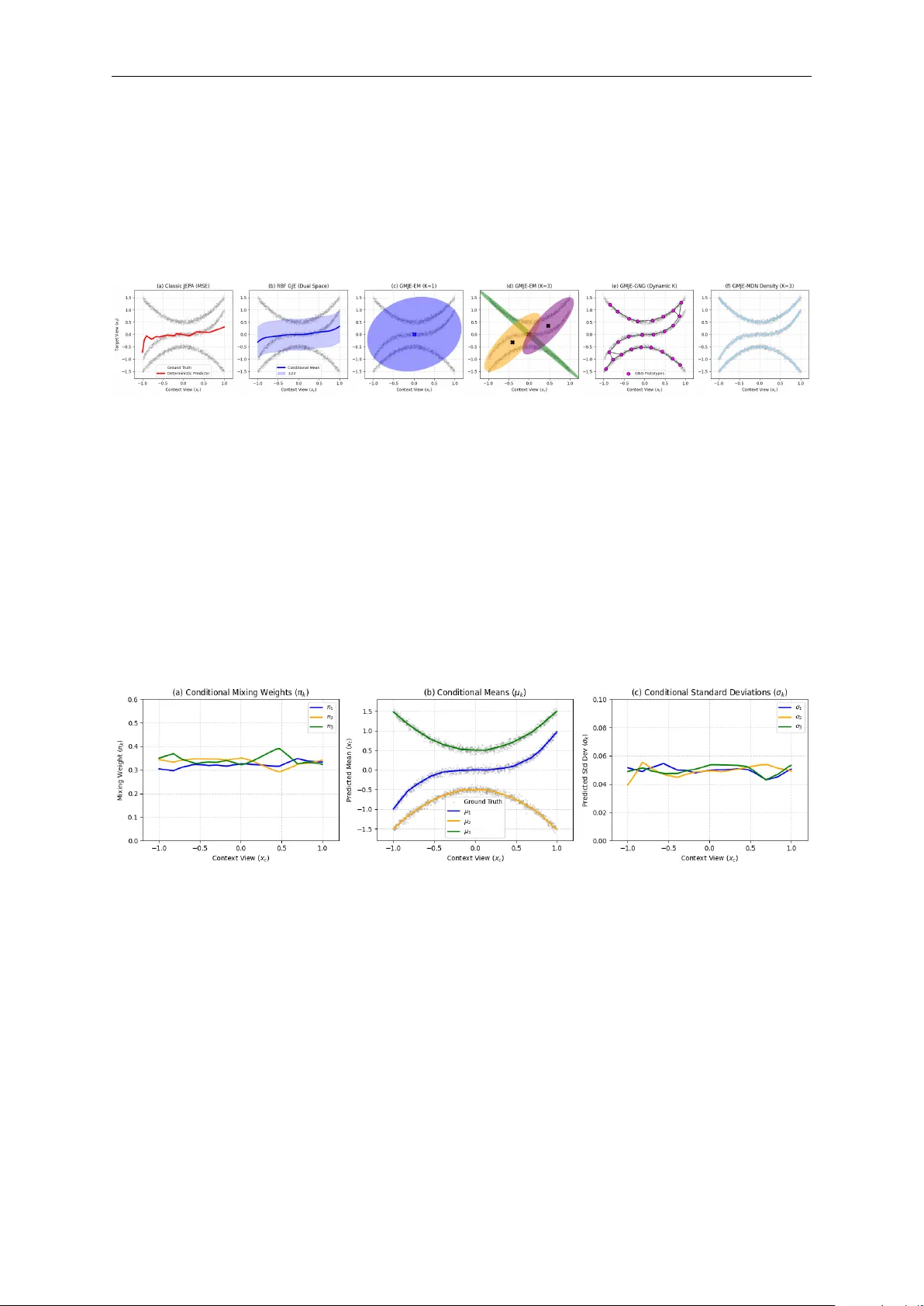
Gaussian Join t Em b eddings F or Self-Sup ervised Represen tation Learning Y ongc hao Huang ∗ 02/03/2026 Abstract Self-sup ervised represen tation learning often relies on deterministic predictive architec- tures to align con text and target views in latent space. While eﬀectiv e in many settings, suc h methods are limited in gen uinely multi-modal in v erse problems, where squared-loss pre- diction collapses to wards conditional a verages, and they frequently depend on architectural asymmetries to prev ent representation collapse. In this work, we prop ose a probabilistic alternativ e based on generativ e joint mo deling. W e in tro duce Gaussian Join t Embeddings (GJE) and its m ulti-mo dal extension, Gaussian Mixture Joint Em b eddings (GMJE), which mo del the joint density of context and target represen tations and replace black-box predic- tion with closed-form conditional inference under an explicit probabilistic mo del. This yields principled uncertaint y estimates and a cov ariance-aw are ob jective for controlling laten t ge- ometry . W e further identify a failure mo de of naive empirical batc h optimization, whic h we term the Mahalanobis T r ac e T r ap , and dev elop sev eral remedies spanning parametric, adap- tiv e, and non-parametric settings, including prototype-based GMJE, conditional Mixture Densit y Netw orks (GMJE-MDN), top ology-adaptive Gro wing Neural Gas (GMJE-GNG), and a Sequen tial Monte Carlo (SMC) memory bank. In addition, we show that standard con trastive learning can b e in terpreted as a degenerate non-parametric limiting case of the GMJE framework. Exp eriments on synthetic m ulti-mo dal alignmen t tasks and vision bench- marks show that GMJE recov ers complex conditional structure, learns competitive discrim- inativ e representations, and deﬁnes latent densities that are b etter suited to unconditional sampling than deterministic or unimo dal baselines. Con ten ts 1 In tro duction 5 2 Bac kground: F rom Deterministic Prediction to Generative Joint Mo deling 6 3 Gaussian Joint Embeddings (GJE) 8 3.1 The Dual F ormulation: Sample-Space Gaussian Pro cess Join t Em b eddings (GPJE) 9 3.2 The Primal F ormulation: F eature-Space Cov ariance . . . . . . . . . . . . . . . . . 10 3.3 Sample Space vs. F eature Space . . . . . . . . . . . . . . . . . . . . . . . . . . . 12 4 (Primal Space) Gaussian Mixture Joint Embeddings (GMJE) 13 4.1 F rom Unimo dal to Multi-mo dal Joint Mo deling . . . . . . . . . . . . . . . . . . . 14 4.2 The GMM F ormulation for Joint Embeddings . . . . . . . . . . . . . . . . . . . . 15 4.3 Scalable Optimization via Learnable Protot yp es . . . . . . . . . . . . . . . . . . . 17 ∗ [Email: yongc hao.huang@abdn.ac.uk] The author welcomes any follow-up work, extensions, and adaptations of these ideas. If this manuscript found useful in future research, appropriate citation w ould b e appreciated. It w as dev elop ed ov er many da ys and nights with the aim of providing a self-contained material for op en knowledge sharing, although some (many) errors may still remain after careful review. 1 In tro | Back | GJE | GMJE | Exp | Disc | Con | Lite | App 4.4 GMJE-MDN: Mixture Densit y Net work (MDN) for GMJE Learning . . . . . . . 20 4.4.1 MDN . . . . . . . . . . . . . . . . . . . . . . . . . . . . . . . . . . . . . . 20 4.4.2 GMJE-MDN . . . . . . . . . . . . . . . . . . . . . . . . . . . . . . . . . . 21 4.5 GMJE-GNG: Dynamic Protot yp e Discov ery via Gro wing Neural Gas . . . . . . . 23 4.5.1 Mathematical F ormulation . . . . . . . . . . . . . . . . . . . . . . . . . . 24 4.5.2 The GNG Algorithm for GMJE Comp onent Learning . . . . . . . . . . . 24 4.6 Data as Mode GMJE (DaM-GMJE): Con trastive Learning as Non-Parametric GMJE . . . . . . . . . . . . . . . . . . . . . . . . . . . . . . . . . . . . . . . . . . 26 4.7 Sequen tial Mon te Carlo (SMC) for Dynamic Memory Bank Optimization . . . . 29 4.7.1 The Memory Bank as a Particle System . . . . . . . . . . . . . . . . . . . 30 4.7.2 Sequen tial Imp ortance W eighting and Resampling . . . . . . . . . . . . . 30 4.7.3 Algorithm: SMC-GMJE for Dynamic Memory Bank Optimization . . . . 31 4.8 Generativ e GMJE: Sampling from the Learned Latent Manifold . . . . . . . . . . 33 5 Exp erimen ts 35 5.1 Am biguous Alignmen t of Synthetic Em b edding Representations . . . . . . . . . . 35 5.2 Represen tation Learning on Vision Benchmarks . . . . . . . . . . . . . . . . . . . 39 5.2.1 The Eﬃciency of SMC Memory Banks vs. FIF O . . . . . . . . . . . . . . 40 5.2.2 SMC-GMJE vs. Standard Baselines . . . . . . . . . . . . . . . . . . . . . 41 5.3 Generativ e GMJE: Unconditional Image Synthesis via Latent Sampling . . . . . 42 6 Discussion 46 7 Conclusion 47 8 Related W orks 48 A Prop erties of Gaussian Distributions 55 A.1 F ormal Deﬁnition and Aﬃne T ransformations . . . . . . . . . . . . . . . . . . . . 56 A.2 Densit y F unction and Geometric In terpretation . . . . . . . . . . . . . . . . . . . 56 A.3 Join t Normalit y vs. Marginal Normality . . . . . . . . . . . . . . . . . . . . . . . 56 A.4 Marginal and Conditional Distributions . . . . . . . . . . . . . . . . . . . . . . . 56 A.5 Information-Theoretic Prop erties . . . . . . . . . . . . . . . . . . . . . . . . . . . 57 A.6 Log-Lik eliho o d and Sampling . . . . . . . . . . . . . . . . . . . . . . . . . . . . . 58 B Blo c k Matrix Inv ersion and Determinant 58 B.1 Blo c k Matrix In version . . . . . . . . . . . . . . . . . . . . . . . . . . . . . . . . . 58 B.2 Blo c k Matrix Determinan t . . . . . . . . . . . . . . . . . . . . . . . . . . . . . . . 59 C Deriv ation of the Conditional Distribution via Aﬃne T ransform, and Joint Distribution and Completing the Square 60 C.1 Method 1: Deriv ation via Aﬃne T ransformation . . . . . . . . . . . . . . . . . . 60 C.2 Method 2: Deriv ation via Joint Distribution and Completing the Square . . . . . 61 C.3 Application to Gaussian Join t Em b eddings (GJE) . . . . . . . . . . . . . . . . . 61 D Primal-GJE Learning Ob jectiv e: Join t vs. Conditional Likelihoo d 62 D.1 The Generativ e Ob jective (Join t NLL) . . . . . . . . . . . . . . . . . . . . . . . . 62 D.2 The Predictiv e Ob jective (Conditional NLL) . . . . . . . . . . . . . . . . . . . . 63 D.3 Join t NLL: Closed-F orm Inference via Blo c k Inv ersion . . . . . . . . . . . . . . . 63 D.4 Com bating Collapse: Why Join t Optimization is Required . . . . . . . . . . . . . 64 In tro | Back | GJE | GMJE | Exp | Disc | Con | Lite | App E Represen tation Collapse in Symmetric Dual GJE 64 E.1 The Ro ot Cause: The Asymmetry of the Conditional Likelihoo d . . . . . . . . . 65 E.2 The Structural Resolution: EMA and Stop-Gradients . . . . . . . . . . . . . . . . 65 F T raining Dual-GJE: Kernel Optimization and EMA 66 F.1 Scalable Dual-GJE via Random F ourier F eatures (RFF) . . . . . . . . . . . . . . 67 F.1.1 Kernel Machines and Bo chner’s Theorem . . . . . . . . . . . . . . . . . . 67 F.1.2 Applying RFF to the Dual GJE Matrix . . . . . . . . . . . . . . . . . . . 67 G T raining Primal-GJE: Symmetric Optimization and the En tropy Fix 68 H Deriv ations of Scalable RFF Matrix Identities 69 H.1 Deriv ation of the RFF W o o dbury Identit y . . . . . . . . . . . . . . . . . . . . . . 70 H.2 Deriv ation of the Log-Determinan t via W einstein-Aronsza jn iden tity . . . . . . . 70 I Primal-GJE: Alternativ e Optimization via the Hilb ert-Sc hmidt Independence Criterion (HSIC) Ob jectiv e 71 I.1 The Cross-Cov ariance Op erator . . . . . . . . . . . . . . . . . . . . . . . . . . . . 71 I.2 Population and Empirical HSIC . . . . . . . . . . . . . . . . . . . . . . . . . . . . 72 I.3 Conv ergence and Appro ximation Rates . . . . . . . . . . . . . . . . . . . . . . . . 72 I.4 HSIC as a Diﬀerentiable Self-Sup ervised Ob jectiv e . . . . . . . . . . . . . . . . . 72 J Exact Dual GJE with a Linear Kernel: The Primal-Dual Equiv alence 73 J.1 Setup and the Empirical Loss . . . . . . . . . . . . . . . . . . . . . . . . . . . . . 73 J.2 Part 1: The Data-Fit T erm via the Push-Through Identit y . . . . . . . . . . . . 73 J.3 Part 2: The Geometric Regularizer via W einstein-Aronsza jn . . . . . . . . . . . . 74 J.4 Conclusion: The Unimo dal Constraint . . . . . . . . . . . . . . . . . . . . . . . . 74 K Prop erties of GMM 75 K.1 Deriv ation of the Marginal Distribution of a Join t GMM . . . . . . . . . . . . . . 75 K.2 Deriv ation of the Conditional Distribution of a Join t GMM . . . . . . . . . . . . 76 K.3 Uncertain ty Quan tiﬁcation: The La w of T otal V ariance . . . . . . . . . . . . . . 77 L MSE Minimization Yields the Conditional Mean 78 L.1 The General Case: Tw o Random V ariables . . . . . . . . . . . . . . . . . . . . . 78 L.2 Application to Classic JEP A . . . . . . . . . . . . . . . . . . . . . . . . . . . . . . 79 M The Iden tity Collapse T rap in Dynamic P arameterization (MDN) 80 M.1 The Naive Joint P arameterization . . . . . . . . . . . . . . . . . . . . . . . . . . 80 M.2 The Pathological Optimum (Iden tity Collapse) . . . . . . . . . . . . . . . . . . . 80 M.3 Empirical Symptoms . . . . . . . . . . . . . . . . . . . . . . . . . . . . . . . . . . 80 M.4 The Resolution: The Conditional Information Bottleneck . . . . . . . . . . . . . 81 N Generalizing SMC to the F ull GMJE Ob jectiv e 81 N.1 The Generalized W eight Up date . . . . . . . . . . . . . . . . . . . . . . . . . . . 81 N.2 Algorithm: General SMC-GMJE . . . . . . . . . . . . . . . . . . . . . . . . . . . 82 O The “Mahalanobis T race” T rap in Empirical Batch Optimization 83 O.1 Case 1: The T rap in Unimo dal Gaussian (Primal-GJE) . . . . . . . . . . . . . . 84 O.2 Case 2: The T rap in GMM (GMJE) . . . . . . . . . . . . . . . . . . . . . . . . . 84 O.3 The Dual Consequences of the T race T rap . . . . . . . . . . . . . . . . . . . . . . 85 O.4 Bey ond the T race T rap: The Log-Determinan t Cheat . . . . . . . . . . . . . . . . 86 In tro | Back | GJE | GMJE | Exp | Disc | Con | Lite | App P Exp erimen tal Details 87 P .1 Shared Computing Environmen t . . . . . . . . . . . . . . . . . . . . . . . . . . . 87 P .2 Exp erimen t 1: Synthetic Am biguous Alignment . . . . . . . . . . . . . . . . . . . 87 P .2.1 Random Seeds . . . . . . . . . . . . . . . . . . . . . . . . . . . . . . . . . 87 P .2.2 Data Generation . . . . . . . . . . . . . . . . . . . . . . . . . . . . . . . . 87 P .2.3 Mo dels and Hyp erparameters . . . . . . . . . . . . . . . . . . . . . . . . . 88 P .3 Exp erimen t 2: Representation Learning on Vision Benchmarks (CIF AR-10) . . . 89 P .3.1 Random Seeds . . . . . . . . . . . . . . . . . . . . . . . . . . . . . . . . . 89 P .3.2 Data Pip eline and Augmentations . . . . . . . . . . . . . . . . . . . . . . 89 P .3.3 Shared Backbone . . . . . . . . . . . . . . . . . . . . . . . . . . . . . . . . 89 P .3.4 Exp erimen t 2a: SMC Memory Banks vs. FIFO . . . . . . . . . . . . . . . 89 P .3.5 Exp erimen t 2b: 200-Ep o c h Benchmark Comparison . . . . . . . . . . . . 90 P .4 Exp erimen t 3: Generative GMJE via Unconditional Latent Sampling on MNIST 90 P .4.1 Random Seeds . . . . . . . . . . . . . . . . . . . . . . . . . . . . . . . . . 90 P .4.2 Data Pip eline . . . . . . . . . . . . . . . . . . . . . . . . . . . . . . . . . . 91 P .4.3 Enco der and Deco der Architectures . . . . . . . . . . . . . . . . . . . . . 91 P .4.4 T raining and Sampling Proto col . . . . . . . . . . . . . . . . . . . . . . . 91 In tro | Back | GJE | GMJE | Exp | Disc | Con | Lite | App 1 In tro duction Recen t progress in Self-Sup ervised Learning (SSL) for high-dimensional data has b een strongly inﬂuenced by joint-em b edding architectures, whic h hav e emerged as a ma jor alternative to reconstruction-based ob jectiv es [3, 2]. The central aim of these frameworks is to enco de struc- turally complex inputs, such as augmented or masked views of an image, into a latent repre- sen tation space in whic h semantically meaningful dep endencies can b e captured and predicted [3, 48]. Within this join t-em b edding paradigm, modern metho ds are commonly divided into t wo broad families: c ontr astive appr o aches , which learn by attracting p ositiv e pairs and rep elling negativ e pairs, and non-c ontr astive or pr e dictive appr o aches , whic h directly align representations across views without explicit negativ e samples [19, 30, 20, 8, 6]. In the contrastiv e paradigm (e.g. InfoNCE [72], SimCLR [19], MoCo [35]), netw orks are trained to increase the similarit y b etw een paired augmented views while decreasing similarity to non-matching instances [72, 19, 35]. While highly eﬀective at instance-lev el discrimination, these metho ds primarily learn augmentation-in v ariant representations and are commonly un- dersto od as balancing t wo geometric eﬀects: alignmen t of p ositiv e pairs and uniformity of the represen tation distribution [73]. Because they t ypically rely on ℓ 2 -normalized embeddings and similarit y-based losses, con trastive metho ds are often analysed on the unit hypersphere, rather than through an explicit mo del of cross-view cov ariance structure [73]. In practice, they can also b e computationally demanding, since strong p erformance often dep ends on access to man y negativ e samples, achiev ed either through very large batch sizes as in SimCLR or momen tum- up dated memory queues as in MoCo [19, 35, 17]. T o reduce the computational and design burdens asso ciated with negative sampling, recent SSL researc h has increasingly explored non-contrastiv e and predictiv e architectures, including BYOL [30] and JEP A-style metho ds [3]. Rather than relying on explicit negativ e pairs, these approac hes learn b y predicting one represen tation from another in laten t space [30, 3]. How ever, deterministic prediction can b e limiting when the c onditional target distribution is gen uinely m ultimo dal. In partial-observ ation or masking settings, a single context representation ma y b e compatible with multiple plausible target representations, esp ecially when the con text do es not uniquely determine the target [10]. Under squared-error risk, the Bay es-optimal determin- istic predictor is the conditional mean, and in multi mo dal problems this av eraging eﬀect can place predictions b et w een mo des, p oten tially in regions that do not corresp ond to t ypical data samples [10, 11]. Moreo ver, unlike contrastiv e ob jectiv es, predictive regression losses do not ex- plicitly enforce a global disp ersion or uniformity constraint on the representation distribution, so additional mec hanisms are often in tro duced to prev ent degenerate solutions during train- ing, including predictor asymmetry , stop-gradient op erations, EMA target netw orks, or explicit v ariance/cov ariance regularization [30, 71, 8, 32]. In this w ork, we prop ose a shift from deterministic laten t prediction to wards gener ative joint mo deling . W e introduce Gaussian Join t Embeddings (GJE) , a probabilistically grounded framew ork that models the concatenated con text and target representations through a joint densit y , p ( z c , z t ). Minimizing the full join t negativ e log-likelihoo d (NLL) yields the standard de- comp osition − log p ( z c , z t ) = − log p ( z t | z c ) − log p ( z c ) , whic h separates a conditional matching term from a marginal densit y term [11]. Under a Gaussian parameterization, the conditional comp onen t encourages agreement b et ween matc hed context-target pairs, while the marginal comp onen t in tro duces co v ariance-dep endent volume r e gularization through the log-determinan t term, promoting a non-degenerate latent geometry . In this sense, GJE is designed to mitigate b oth instanc e c ol lapse and dimensional c ol lapse by explicitly modelling v ariance and cov ariance structure, thereby reducing reliance on architectural asymmetries suc h as EMA target netw orks or stop-gradient mec hanisms that are commonly used in non-contrastiv e SSL [30, 8, 71]. Because a single Gaussian density is often to o restrictive to represent multi-modal or highly non-con vex laten t structure, we further extend this GJE formulation and in tro duce Gaussian In tro | Back | GJE | GMJE | Exp | Disc | Con | Lite | App Mixture Join t Em b eddings (GMJE) . By lev eraging the expressiv e p o wer and universal appro ximation prop erties of Gaussian mixture mo dels [50, 39], GMJE can represent highly ir- regular and multi-modal semantic structure more ﬂexibly than a single-Gaussian joint mo del [26, 51]. Imp ortantly , we identify a failure mo de that can arise when naiv ely implementing probabilistic joint-em b edding ob jectiv es, whic h we term the Mahalanobis T r ac e T r ap . Speciﬁ- cally , we show that when joint likelihoo ds are computed using empirical batch cov ariances, the resulting Mahalanobis coupling term can degenerate so that the intended cross-view attractive signal b ecomes constant, thereb y weak ening cross-view learning. T o address this failure mo de, w e introduce three GMJE arc hitectural remedies spanning b oth parametric and non-parametric settings. Ultimately , we show that GMJE can learn strong discriminativ e represen tations while sim ultaneously deﬁning a con tinuous probabilistic densit y ov er the latent space, which can b e used for subsequen t discriminativ e or generative tasks. In summary , our core contributions are as follo ws: - A new probabilistic paradigm: w e formalize the GJE framework and show that re- placing conditional MSE prediction with join t generative mo deling yields closed-form conditional predictions, uncertaint y estimates, and an ob jective with built-in v ariance- co v ariance con trol that can mitigate representation collapse while reducing reliance on arc hitectural asymmetries. - Multi-modal extension via GMJE: we introduce Gaussian Mixture Join t Em b eddings (GMJE) to address the unimodal limitations of single-Gaussian GJE. T o optimize this ric her joint distribution while av oiding the Mahalanobis T r ac e T r ap , we dev elop sev eral GMJE v ariants spanning parametric, adaptive, and non-parametric settings, including learnable global prototypes, conditionally dynamic Mixtur e Density Networks (GMJE- MDN), top ology-adaptiv e Gr owing Neur al Gas (GMJE-GNG), and the non-parametric SMC-GMJE formulation. - The InfoNCE bridge and SMC memory banks: w e establish a theoretical connec- tion showing that standard contrastiv e learning can b e interpreted as a degenerate, non- parametric limiting case of our GMJE framework. Building on this view, we in tro duce Se quential Monte Carlo (SMC) particle ﬁltering, whic h replaces unw eighted contrastiv e FIF O queues, as an alternativ e memory-bank mechanism, yielding dynamically weigh ted samples that prioritize more informativ e samples. - Generativ e laten t densities: we empirically sho w that GMJE learns a contin uous laten t density that is more amenable to generative sampling than standard predictive or con trastive laten t spaces. In our laten t-sampling exp erimen ts, this supp orts unconditional image synthesis through direct sampling from the learned latent distribution. 2 Bac kground: F rom Deterministic Prediction to Generativ e Join t Mo deling In Join t Embedding Predictiv e Architectures (JEP A), the learning ob jectiv e is to predict a target represen tation from a context representation in latent space, typically using a parameterized predictor netw ork. In image-based JEP A, this is implemented b y predicting the representations of masked or spatially separated target blo c ks from an informativ e con text blo c k within the same image [3]. Despite its empirical success, classic JEP A still exhibits several conceptual and arc hitectural limitations: - Deterministic without Unc ertainty: classic JEP A is typically trained with a deterministic regression-st yle ob jective (e.g. MSE) in laten t space. Under squared-error risk, the Ba yes- optimal predictor is the conditional mean E [ z t | z c ]; hence, in gen uinely multi-modal In tro | Back | GJE | GMJE | Exp | Disc | Con | Lite | App x c x t E θ E θ ′ predictor g ( · ) ε D ( ˆ z t , z t ) z c z t × sg ˆ z t (a) x c x t E θ E θ ′ Join t Mo deling parameterized by ( θ , θ ′ ) optimized via joint likelihoo d p ( z c , z t ) ε (optional) z c z t (b) Figure 1: A comparison of (a) the classic JEP A framework, based on separate enco ding and alignmen t via deterministic latent prediction, and (b) our prop osed GJE framework, which mo dels the join t distribution of con text and target represen tations and deriv es predictions prob- abilistically . The comp onen t with a red outline in (a) represents the deterministic distance loss sp eciﬁc to classic JEP A. ‘sg’ denotes stop gr adient , and ε represents injected side information (e.g. ph ysics, action conditioning or noise). settings, deterministic prediction can a verage across mo des and pro duce represen tations that do not corresp ond to typical targets. Because no conditional distribution is mo deled explicitly , this formulation do es not natively pro vide predictiv e uncertain ty estimates [10, 11]. - R isk of R epr esentation Col lapse: standard JEP A do es not explicitly optimize a join t densit y ov er ( z c , z t ) and therefore do es not include a separate marginal densit y term suc h as − log p ( z c ). As a result, unlike ob jectiv es that explicitly control v ariance or cov ariance structure, it do es not directly imp ose a global disp ersion constraint on the representation distribution, which can make collapse av oidance more delicate in practice [8, 71, 32]. - T r aining Stability Me chanisms: as in other non-con trastive join t-embedding methods, stable training often relies on arc hitectural asymmetries or auxiliary regularization mech- anisms. In related predictiv e SSL frameworks, these include stop-gradient op erations, predictor asymmetry , and slow-mo ving target netw orks up dated by exp onen tial moving a verages (EMA) [30, 20, 71]. - Dir e ctional Constr aints: standard JEP A is t ypically form ulated as a uni-directional pre- diction problem ( z c → z t ). Recent work has explored bi-directional extensions, such as BiJEP A [40], to impro ve symmetry and generalization. How ever, it suggests that symmet- ric prediction can amplify optimization instability and may require explicit norm control, suc h as L 2 -normalization, to prev ent represen tation explosion [40]. A comparison of the classic JEP A and our proposed GJE framew ork is sho wn in Fig. 1. GJE replaces deterministic latent prediction with generative join t mo deling: instead of learning only a predictor g ( z c ), w e mo del the concatenated represen tations [ z c , z t ] T through a joint distribution. Under this view, prediction is derived from the learned dep endency structure rather than solely from a black-box predictor. By optimizing a full join t ob jectiv e, GJE explicitly retains v ariance- co v ariance structure that is absent from purely deterministic prediction losses, and is therefore designed to promote a more diverse and non-degenerate embedding geometry . Notation and T erminology . Throughout this work, w e use the following mathematical notations. In tro | Back | GJE | GMJE | Exp | Disc | Con | Lite | App - Data and Emb e ddings: lo wercase letters ( x c , x t ) denote raw individual con text and target views (e.g. augmen ted images). z c , z t ∈ R d denote their resp ectiv e d -dimensional latent represen tations 1 , and Z = [ z T c , z T t ] T denotes the concatenated join t embedding. Upp ercase letters ( Z c , Z t ) represent matrices containing ﬁnite batches of these em b eddings. - Pr ob abilistic Par ameters: Σ denotes the general, theoretical p opulation co v ariance matrix of a multiv ariate distribution, while µ denotes the mean v ector. F or mixture mo dels, π k represen ts the mixture w eight for component k , and γ k ( · ) represents the data-dep enden t p osterior probabilit y (soft routing resp onsibilit y). - Structur al Cap acities ( N , M , K ): to strictly distinguish b etw een optimization batc hes, global memory , and mo del capacity , we deﬁne: ◦ N : the b atch size , i.e. the num b er of current representations pro cessed in a single forw ard pass. ◦ M : the memory b ank size , i.e. the massiv e queue of cached target representations, used in contrastiv e learning and SMC. ◦ K : the numb er of c omp onents/pr ototyp es in a Gaussian Mixture Mo del (GMM). - The Dual Me aning of K and Σ : in Section.3, when discussing dual-GJE, K is exceptionally used to denote the empirical blo ck Gr am matrix computed ov er a batch via a p ositiv e-deﬁnite k ernel function (e.g. K cc , K tt ). Thus, in Section.3, Σ and K represent the same structural concept, distinguishing b et w een pure probabilistic theory (Σ) and empirical kernel-based com- putation ( K ). Everywhere else in the manuscript (Section.4 onw ards), scalar K strictly refers to the n umber of mixture comp onen ts. 3 Gaussian Join t Em b eddings (GJE) T o mo del the alignmen t b et ween a context view x c and a target view x t , w e introduce the Gaussian Joint Emb e dding (GJE) framework. As shown in Fig.1, the input views are passed through a context enco der E θ and a target enco der E θ ′ to pro duce laten t em b eddings z c = E θ ( x c ) ∈ R d c and z t = E θ ′ ( x t ) ∈ R d t . Although the general GJE framework can naturally incorp orate optional side information ε (suc h as ph ysical constraints, action v ariables in reinforcemen t learning, or noise parameters) b y conditioning the joint distribution, in the following w e fo cus on unconditional representation alignmen t. Let z = [ z T c , z T t ] T ∈ R d , where d = d c + d t , denote the concatenated joint em b edding pair. W e assume these representations are dra wn from an underlying joint probability distribu- tion p ( z ; θ , θ ′ ) parameterized by the neural enco ders. The self-sup ervised ob jective is then to optimize the enco der parameters b y maximizing the exp ected join t log-likelihoo d o ver matc hing pairs ( x c , x t ) drawn from the dataset D : max θ,θ ′ E ( x c ,x t ) ∼D [log p ( E θ ( x c ) , E θ ′ ( x t ))] (1) By the c hain rule of probability , the joint ob jective factorizes as log p ( z c , z t ) = log p ( z t | z c ) + log p ( z c ) , whic h may b e in terpreted as a predictive conditional term together with a marginal regulariza- tion term. T o mak e this optimization computationally tractable and geometrically meaningful, w e imp ose a Gaussian assumption on the em b edding space. Depending on how this Gaussian 1 Note: in the brief literature review of Mixture Density Netw orks in Section.4.4.1, we temp orarily preserve Bishop’s original use of c to denote dimensionality to maintain historical ﬁdelity . In tro | Back | GJE | GMJE | Exp | Disc | Con | Lite | App structure is instantiated, the framework can b e developed from tw o complementary p ersp ec- tiv es: the dual (sample) view , which fo cuses on the predictive conditional alignment p ( z t | z c ) o ver a batch of N points, and the primal (fe atur e) view , which mo dels the full joint density p ( z c , z t ) natively o ver the d laten t dimensions. 3.1 The Dual F ormulation: Sample-Space Gaussian Pro cess Joint Embed- dings (GPJE) In classic JEP A, a deterministic neural predictor maps the context em b edding to the target em b edding: ˆ z t = g ( z c ). T o generalize this probabilistically , we ﬁrst formulate the problem in the dual sample sp ac e b y replacing this parametric MLP with a non-parametric probabilistic regression mo del, which treats the target embedding z t as a realization of an underlying latent function f ev aluated at the context embedding z c : z t = f ( z c ) + ϵ, ϵ ∼ N ( 0 , σ 2 I ) (2) Here, f ∼ G P ( 0 , k ( z c , z ′ c )) is a Gaussian Pro cess deﬁned by a p ositiv e-deﬁnite kernel k , whic h dictates that cov( f ( z c ) , f ( z ′ c )) = k ( z c , z ′ c ). Rather than mo deling the cov ariance b et w een the d feature channels, this sample-space GP mo dels the similarities b etw een the individual data p oin ts. 1. T raining (The Joint Likelihoo d). During training, we extract a batc h of N con text and target embedding pairs, Z c ∈ R N × d c and Z t ∈ R N × d t . W e compute the Gram matrix K cc ∈ R N × N o ver the con text embeddings, where each element K cc [ i, j ] = k ϕ ( z c,i , z c,j ), capturing the non-linear top ological distances b et w een ev ery sample in the batch. T reating the target embeddings Z t ∈ R N × d t as the observed function v alues, we derive the training ob jectiv e b y assuming the d t laten t feature c hannels are indep enden t Gaussian Pro cesses sharing the same context k ernel K cc . F or a single feature channel (represen ted as a column v ector z t,j ∈ R N × 1 ), the standard GP negative marginal log-likelihoo d, assuming negligible observ ation noise and dropping constant scaling terms, is 2 1 2 z T t,j K − 1 cc z t,j + 1 2 log | K cc | . Summing this indep enden t ob jectiv e across all d t target dimensions yields the total joint negative log-lik eliho o d. In linear algebra, the summation of these data-ﬁt quadratic forms across all column vectors mathematically condenses in to a matrix trace op erator ( P d t j =1 z T t,j K − 1 cc z t,j = T r( Z T t K − 1 cc Z t )). Meanwhile, the data-indep endent log-determinant p enalt y simply accum ulates d t times. Th us, the ﬁnal Dual-GJE ob jectiv e used to optimize the enco der weigh ts is: L Dual-GJE ( θ , θ ′ , ϕ ) = 1 2 T r  Z T t K − 1 cc Z t  | {z } Data-Fit + d t 2 log | K cc | | {z } Complexity Penalty (3) This Dual-GJE optimisation ob jective is a c onditional NLL 3 , p ( Z t | Z c ). As this GP marginal lik eliho o d is inheren tly asymmetric - it p enalizes the volume of the context space (log | K cc | ) but applies no such expansive regularizer to the target space, optimizing Eq.3 symmetrically w ould result in catastrophic represen tation collapse. The target enco der w ould trivially map Z t → 0 to minimize the quadratic trace p enalt y , subsequently causing the log-determinant to collapse the context space 4 . T o eﬀectively optimize this dual ob jectiv e, the target enco der E θ ′ m ust b e maintained as 2 See Eq.(2.29) and Eq.(2.30) in [63]. W e dropp ed the constant term. 3 See Eq.(2.29) or Eq.(2.30) in [63]. 4 A detailed explanation of this learning collapse can b e found in App endix.E. In tro | Back | GJE | GMJE | Exp | Disc | Con | Lite | App an Exp onen tial Moving Average (EMA) [30, 20, 3, 41] of the context enco der 5 , with a strict stop-gradien t applied to Z t . By anchoring the targets, Z t acts as a diverse, ﬁxed top ological reference. Only under this asymmetric EMA framework do es the trace term correctly function as an expansionary force, comp elling the context em b eddings to spread out and strictly match the pairwise diversit y of the targets, while the log-determinant term acts as an Occam’s razor, regularizing the con text manifold to remain smo oth. If explicit homoscedastic observ ation noise σ 2 I is mo deled, the ob jective Eq.3 expands to: L JEGP ( θ , θ ′ ) = 1 2 T r  ( K cc + σ 2 I ) − 1 Z t Z T t  + d t 2 log | K cc + σ 2 I | (4) By the cyclic prop ert y of the trace op erator (T r( AB ) = T r( B A )), the data-ﬁt terms in Eq.3 and Eq.4 are mathematically equiv alent. Both formulations drive the exact same geometric forces, optimizing the enco ders symmetrically . The Dual-GJE algorithm is presented in Algo.3 in App endix.F; a scalable Dual-GJE via Random F ourier F eatures (RFF) is presented in the same app endix. 2. Inference (The Conditional Prediction). Once the enc o ders and kernel ar e tr aine d , w e freeze the training memory bank Z t ∈ R N × d t and the training Gram matrix K cc ∈ R N × N . Giv en a brand new, unobserv ed test con text image x ∗ c , w e map it to a single embedding z ∗ c ∈ R 1 × d c . W e compute its cross-similarit y v ector against all N training samples, k ∗ c ∈ R 1 × N , and its self-similarity scalar k ∗∗ ∈ R 1 × 1 . Using the Sch ur complement to condition the join t GP distribution, the predictiv e distribution for the target z ∗ t ∈ R 1 × d t is exactly Gaussian, N ( µ t | c , Σ t | c ), deﬁned b y 6 : µ t | c = k ∗ c K − 1 cc Z t Σ t | c = k ∗∗ − k ∗ c K − 1 cc k c ∗ (5) Notice the dimensions of Eq.5: [1 × N ] × [ N × N ] × [ N × d t ] = [1 × d t ]. The prediction is a non- parametric, weigh ted a verage ov er (i.e. linear com bination of ) the entire training memory bank Z t . (Note: Be c ause exact inversion r e quir es O ( N 3 ) c ompute, GJE supp orts a highly sc alable R andom F ourier F e atur e (RFF) appr oximation, detaile d in App endix.F.1). 3.2 The Primal F orm ulation: F eature-Space Cov ariance While the dual form ulation ev aluates sample similarit y , the primal formulation ev aluates the geometric shap e of the data manifold itself by measuring how the d latent features co-v ary . 1. T raining and the Mahalanobis T race T rap. W e concatenate the con text and target batc hes in to a single joint batch Z = [ Z c , Z t ] ∈ R N × d . W e assume a joint, zero-mean Multiv ari- ate Gaussian generative mo del p ( z ) = N ( 0 , C j oint ), i.e. each concatenated embedding vector z i ∈ R d is drawn from this Gaussian distribution: p ( z i ) ∼ N ( z | 0 , C j oint ) = 1 p (2 π ) d | C j oint | exp  − 1 2 z T C − 1 j oint z  (6) 5 In standard Join t Embedding Architectures, the target enco der weigh ts θ ′ are typically up dated as an Exp o- nen tial Moving Average (EMA) of the context enco der weigh ts θ , such that θ ′ ← τ θ ′ + (1 − τ ) θ where τ ∈ [0 , 1) is a momentum parameter. This asymmetric weigh t up date, com bined with a stop-gr adient operation on the target branch, is a crucial architectural heuristic in mo dels such as BYOL [30] and standard JEP A [3] to preven t represen tation collapse - a failure mode where the net work maps all inputs to a trivial constan t v ector to perfectly minimize prediction error. 6 See Eq.(2.25) and Eq.(2.26) in [63]. If explicit homoscedastic observ ation noise is mo deled (as in Eq.4), the predictiv e distribution seamlessly adapts by replacing the in verse Gram matrix K − 1 cc in b oth equations with the noise-regularized term ( K cc + σ 2 I ) − 1 . In tro | Back | GJE | GMJE | Exp | Disc | Con | Lite | App In the context of deep represen tation learning, this strict zero-mean assumption serves a critical regularizing function: it anc hors the laten t space at the origin and forces the enco ders to delegate all structural learning en tirely to the co v ariance matrix. This preven ts the netw ork from trivially minimizing the loss via arbitrary translational mean shifts. Consequen tly , the feature cov ariance matrix C j oint , with dimension d × d , can be empirically 7 computed directly from the origin for the N training data p oin ts 8 : C j oint = 1 N Z T Z ∈ R d × d (7) and it can b e partitioned in to four blo cks: C j oint =  C cc C ct C tc C tt  (8) where C cc ∈ R d c × d c and C tt ∈ R d t × d t are the auto-cov ariances, and C ct ∈ R d c × d t is the cross- co v ariance capturing mutual information. Inv erting C j oint can b e done using blo c k matrix in version and the Sc hur complemen t (see Eq.62 in App endix.D). Assuming the N samples in the mini-batch are indep enden t and identically distributed, the likelihoo d of the entire empirical batc h is the pro duct of the individual densities, p ( Z ) = Q N i =1 p ( z i ). T o optimize the encoder parameters, w e formulate the empirical av erage of the NLL, deﬁned as − 1 N log p ( Z ): − 1 N log N Y i =1 p ( z i ) = − 1 N N X i =1 log p ( z i ) = 1 N N X i =1  1 2 z T i C − 1 j oint z i + 1 2 log | C j oint | + d 2 log(2 π )  Dropping the constan t d 2 log(2 π ) term, which has no eﬀect on the gradient with resp ect to the net work weigh ts, the strict generative ob jectiv e minimizing the exact NLL ov er this d × d space b ecomes: L Primal-GJE ( θ , θ ′ ) = 1 2 N N X i =1 z T i C − 1 j oint z i + 1 2 log | C j oint | (9) F rom an information-theoretic p erspective, minimizing this joint ob jective natively maximizes the Mutual Information b et ween the con text and target spaces while regularizing their diﬀer- en tial en tropy . F urther, factoring this join t lik eliho o d shows why conditional-only arc hitectures lik e classic JEP A require asymmetric heuristics to survive (for formal pro ofs, see App endix.D). It seems from the primal ob jectiv e Eq.9 that, minimizing the volume penalty log | C j oint | na- tiv ely enforces compression, while the in verted Mahalanobis distance acts as a repulsive force; ho wev er, directly optimizing this exact NLL in the empirical primal space rev eals a fatal opti- mization trap. Because the scalar quadratic form is equal to its own trace, we can apply the cyclic prop ert y (T r( AB ) = T r( B A )) to the data-ﬁt term: 1 2 N N X i =1 T r( z T i C − 1 j oint z i ) = 1 2 T r C − 1 j oint " 1 N N X i =1 z i z T i #! = 1 2 T r( C − 1 j oint C j oint ) = d 2 The inv erted Mahalanobis distance algebraically cancels against the empirical cov ariance, col- lapsing the entire data-ﬁt term into a dead constant scalar d 2 . With a constant data-ﬁt term, 7 F or simplicity , we use the same notation C j oint for the p opulation and empirically estimated cov ariance matrix. 8 By treating the data matrix Z ∈ R N × d as a stack of N row vectors Z = [ z T 1 , z T 2 , . . . , z T N ] T , its trans- p ose Z T ∈ R d × N b ecomes a matrix of side-by-side column v ectors Z T = [ z 1 , z 2 , . . . , z N ]. Using blo c k matrix m ultiplication, multiplying the row of blo c ks by the column of blo c ks yields the sum of their outer pro ducts: Z T Z = [ z 1 , . . . , z N ][ z T 1 , . . . , z T N ] T = P N i =1 z i z T i . T aking the a verage with N or N − 1 is trivial. In tro | Back | GJE | GMJE | Exp | Disc | Con | Lite | App the expansive gradien t is exactly zero. The optimizer is left solely with the volume p enalty (+ 1 2 log | C j oint | ), which it trivially minimizes by shrinking all represen tations to the origin, causing catastrophic dimensional collapse (details ab out The “ Mahalanobis T r ac e T r ap ” see App endix.O). Therefore, to maintain stable represen tations in the primal space, w e cannot rely on the nativ e Mahalanobis distance for repulsion. W e must structurally inv ert the regularizer, i.e. maximizing the diﬀeren tial entrop y 1 2 log | C j oint | to force the features to span the av ailable v olume [8], or alternativ ely , optimize the cross-cov ariance directly via the Hilb ert-Schmidt In- dep endence Criterion (see App endix.I). The Primal-GJE algorithm is presen ted in Algo.5 in App endix.G. 2. Inference (The Closed-F orm Linear Predictor). After training, we freeze the four d × d cov ariance blo c ks. Given a new test context vector z ∗ c ∈ R d c × 1 (formatted as a column v ector), the conditional distribution p ( z ∗ t | z ∗ c ) = N ( z ∗ t | µ t | c ( z ∗ c ) , Σ t | c ) is analytically derived via blo c k matrix in version (deriv ations in App endix.B): µ t | c = C tc C − 1 cc z ∗ c Σ t | c = C tt − C tc C − 1 cc C ct (10) In Eq.10, the term ( C tc C − 1 cc ) multiplies a [ d t × d c ] matrix by a [ d c × d c ] matrix, resulting in a ﬁxed [ d t × d c ] weigh t matrix. Therefore, the primal GJE form ulation mathematically derives the optimal line ar pr oje ction layer directly from the global feature co v ariances, requiring no training data in memory during inference 9 . It is observed that, the predictive v ariance is a constan t decided by the training set, and it’s indep endent of the test context z ∗ c . 3.3 Sample Space vs. F eature Space The Dual GJE (Section.3.1) and the Primal GJE (Section.3.2) b oth rely on the fundamental Gaussian assumption, but they approach the z c → z t mapping problem from p erp endicular geometric p ersp ectiv es. Dual GJE (GPJE) operates in the sample space, asking the geometric question: “how similar is Image A to Image B?” By ev aluating the N × N Gram matrix computed via inner pro ducts betw een samples (e.g. K cc ∝ Z c Z T c ), this view do es not mo del individual features, but rather collapses feature v ectors into holistic similarity scores. It formulates the predictor as a non-parametric Gaussian Process, assuming the target em b eddings Z t are join tly Gaussian with a co v ariance structure determined b y these kernel similarities of their contexts. The resulting predictiv e distribution (Eq.5) is dynamic; its conditional mean and v ariance depend on b oth the stored training instances and the top ological distance of the sp eciﬁc test context z ∗ c . Ho wev er, as an instance-based memory mo del, ev aluating the GPJE ob jectiv e (Eq.3) requires inv erting an N × N matrix, imp osing a sev ere O ( N 3 ) computational b ottlenec k. F urther, as the GP marginal likelihoo d is strictly a c onditional ob jectiv e 10 p ( Z t | Z c ), it lacks a native volume regularizer for the context space, thereby mandating asymmetric heuristics lik e EMA target net works to preven t representation collapse. Primal GJE , conv ersely , op erates in the feature space, asking the p erpendicular question: “ho w similar are the individual latent features to eac h other across the dataset?” It acts as a parametric mo del. It assumes a single, unimo dal joint Gaussian distribution (Eq.6) o ver the concatenated feature space. By computing the inner pro ducts b et ween the features themselves, its empirical cov ariance matrix C j oint ∝ Z T Z has dimension d × d , whic h, for typical mo dern em b edding sizes where d ≪ N , is massiv ely smaller and computationally c heap er to inv ert 9 T raining data info is summarised in the matrices [ C cc , C ct , C tc , C tt ] via Eq.7 10 see Eq.(2.29) or Eq.(2.30) in [63]. In tro | Back | GJE | GMJE | Exp | Disc | Con | Lite | App ( O ( d 3 )) than the dual Gram matrix. In this primal view, the resulting conditional prediction (Eq.10) yields a mean that linearly dep ends on the test context z ∗ c , but a predictive cov ariance that is strictly constan t, frozen entirely by the global distribution of the training data. Crucially , b ecause it optimizes the full joint likelihoo d 11 p ( z c , z t ), it provides native, symmetric regularizers for b oth the context and target spaces, eliminating the strict requirement for asymmetric stop- gradien ts. The Primal-Dual Equivalenc e. While they approac h the geometry from diﬀeren t dimen- sions, the tw o formulations are fundamentally link ed. In fact, if the non-parametric Dual-GJE is implemented using a standard linear kernel, the exact O ( N 3 ) Gaussian Pro cess NLL alge- braically collapses en tirely in to the O ( d 3 ) Primal-GJE co v ariance matrix framew ork (pro of see App endix.J). This strict primal-dual equiv alence mathematically pro ves that, without the use of computationally exp ensiv e non-linear kernel appro ximations (such as RBF or RFF), the dual sample-space optimization lo c ks the latent geometry to the exact same single, rigid density as the primal feature space 12 . Unimo dalit y and Homoscedasticity Issues Regardless of whether GJE is form ulated in the non-parametric dual space (Eq.5) or the parametric primal space (Eq.10), b oth architectures suﬀer from a shared limitation: unimo dality . Because b oth form ulations rely on a single join t Gaussian structure, they can only issue a unimo dal predictiv e distribution. Consequently , when faced with diverging semantic branches, i.e. when there are m ultiple options for z ∗ t for a given z ∗ c , the predictive mean µ t | c is mathematically forced to predict the literal a verage of the mo des (slicing through empty space, see pro of in App endix.L). Neither mo del can physically route predictions to distinct, isolated target branches (a failure case we w ill see later in a syn thetic example in Section 5). F urther, the parametric primal-GJE is constrained by homosc e dasticity . While the dual-GJE yields a dynamic, distance-aw are predictive co v ariance 13 that changes based on the test context z ∗ c , the primal-GJE predictiv e cov ariance (Σ t | c in Eq.10) is a rigid, constan t matrix determined en tirely b y the global training distribution. It contains no reference to the sp eciﬁc input z ∗ c . Th us, to blanket the multi-modal spread of am biguous inputs, the primal-GJE mo del must globally inﬂate its static v ariance across the en tire latent space, degrading predictive certaint y ev en for unambiguous samples. These structural limitations, i.e. the inability to mo del multiple target branches and the rigid cov ariance of the parametric space, motiv ate our transition to Gaussian Mixture Joint Em b eddings (GMJE) in the primal feature space. 4 (Primal Space) Gaussian Mixture Join t Em b eddings (GMJE) GJE is strictly unimo dal regardless of the k ernel used; either classic JEP A or GJE can solve m ulti-mo dal alignment 14 . In this section, we present the feature (primal) space Gaussian Mix- tur e Joint Emb e ddings (GMJE), a fully generalized, probabilistically grounded framework for m ulti-mo dal representation learning. W e ﬁrst motiv ate the transition from unimo dal to multi- mo dal joint mo deling and establish the universal approximation capabilities of Gaussian mix- tures. Next, we deﬁne the general GMJE formulation (Section.4.2), demonstrating how it uses a joint mixture mo del to natively capture complex dep endencies and m ulti-mo dal alignments. The remainder of the section in tro duces a suite of principled metho dologies to optimize this join t 11 See App endix.D a comparison of the joint and conditional NLL op jectives. 12 The surprise comes as: with a linear kernel, Dual is exactly equal to Primal. Therefore, they b oth suﬀer from the exact same Unimo dal Gaussian T rap. 13 Standard Gaussian Pro cess regression is heteroscedastic with resp ect to distance (the v ariance grows as the test p oin t mov es further from the training data, b ecause k ∗ c go es to zero and we are left with the prior v ariance k ∗∗ ). 14 W e present an ambiguous multi-modal alignment task in Section.5.1 to illustrate this. In tro | Back | GJE | GMJE | Exp | Disc | Con | Lite | App distribution, naturally divided into parametric and non-parametric branc hes. In the paramet- ric branc h, we explore a highly scalable approach using r elaxe d Exp e ctation-Maximization with ﬁxed global prototypes (Section.4.3), extend it to instance-conditioned parameter generation via Mixtur e Density Networks (Section.4.4), and resolv e the need for a predeﬁned num b er of comp onen ts using dynamic top ology mapping via Gr owing Neur al Gas (Section.4.5). Finally , in the non-p ar ametric branc h, w e provide a theoretical pro of linking GMJE to Contrastiv e Learn- ing (Section.4.6), which motiv ates our solution to memory bank optimization using a dynamic Se quential Monte Carlo (SMC) particle ﬁlter (Section.4.7). 4.1 F rom Unimo dal to Multi-mo dal Joint Mo deling While the single Gaussian assumption in GJE pro vides an elegant closed-form predictor (cc.Eq.10), its op eration in the dual sample space structurally restricts the conditional distribution p ( z t | z c ) to a single, unimo dal pro jection. In standard self-supervised tasks, the true distribution of v alid target views giv en a con text view is inheren tly multi-mo dal . F or example, a heavily masked im- age of a dog’s face ( x c ) could v alidly b e completed in to several distinct p ostures, breeds, or bac kgrounds ( x t ). A unimo dal pro jection ov er-smo othes these relationships, forcing the pre- dicted mean to lie somewhere in the empty space b etw een v alid mo des. T o capture the complex, m ulti-mo dal alignmen t of representati ons, we extend GJE to Gaus- sian Mixtur e Joint Emb e ddings (GMJE), switching from dual sample space view to the primal feature space view. Ho wev er, note that GJE (sample space) and GMJE (feature space) are not directly comparable in their capacities. Before detailing our sp eciﬁc join t formulation, we ﬁrst establish the foundational p ow er of Gaussian Mixture Mo dels (GMMs). A general GMM with K comp onen ts is deﬁned as [64]: q θ ( z ) = K X i =1 w i N ( z | µ i , Σ i ) (11) where the parameters θ = { w i , µ i , Σ i } K i =1 consist of mixture w eights ( w i ≥ 0, P K i =1 w i = 1), means ( µ i ∈ R d ), and p ositiv e deﬁnite co v ariance matrices ( Σ i ∈ R d × d ). The transition to a mixture-based approac h is mathematically justiﬁed by the profound represen tational capacit y of GMMs, formally stated in the follo wing univ ersal densit y appro xi- mation prop ert y [50]: Theorem 1 (Universal approximation prop ert y of GMMs [50, 39]) . A ny suﬃciently smo oth pr ob ability density function p ( z ) on R d c an b e appr oximate d arbitr arily closely in L 1 distanc e by a Gaussian Mixtur e Mo del (GMM) with a ﬁnite, suﬃciently lar ge numb er of c omp onents c overing its whole supp ort. Pr o of. (sk etc h) According to results in mixture density estimation theory (e.g. Li & Barron [50], Norets [57]), the set of Gaussian mixtures is dense in the space of contin uous densities with resp ect to the L 1 norm, provided p ( z ) has b ounded supp ort or decays suﬃciently fast at inﬁnit y (e.g. faster than an y Gaussian tail). Let ϵ > 0 b e the desired approximation error. The L 1 distance 15 b et w een the true densit y 15 In density estimation, the Kullback-Leibler (KL) divergence b et ween tw o densities is often used due to its in trinsic connection with maximum likelihoo d. How ever, the L 1 norm is utilized in this theoretical analysis for t wo primary reasons [39]: its practical probabilistic meaning and its conv enient mathematical prop erties for error decomp osition. (1) Probabilistic interpretation: the L 1 norm has a direct and intuitiv e connection to ho w distinguishable tw o probability distributions are - it is equal to t wice the T otal V ariation (TV) distance: ∥ p − q ∥ L 1 = 2 · D T V ( p, q ). The TV distance represents the largest p ossible diﬀerence in probability that the t wo distributions can assign to any single ev ent. F or example, if ∥ p − q ∥ L 1 = 0 . 1, then the TV distance is 0 . 05. This guarantees that for an y p ossible even t, the probabilities calculated b y p and q will diﬀer by at most 5%. (2) Mathematical prop erties for analysis: unlike KL divergence, the L 1 norm is a true metric , satisfying In tro | Back | GJE | GMJE | Exp | Disc | Con | Lite | App p ( z ) and the approximation q θ ( z ) is deﬁned as 16 : ∥ p − q θ ∥ L 1 = Z Z | p ( z ) − q θ ( z ) | d z By the deﬁnition of this denseness prop erty in L 1 space, there must exist a ﬁnite K and a parameter set θ such that ∥ p − q θ ∥ L 1 < ϵ . The required num b er of comp onen ts K dep ends purely on the target’s geometric complexity (e.g. its curv ature and num b er of mo des). Therefore, a GMM with ﬁnite K can approximate an y contin uous target density within an arbitrary ϵ - error b ound, mathematically justifying the use of Gaussian mixtures as a ﬂexible, universal represen tation capable of mapping the highly irregular distributions found in self-sup ervised learning. Corollary 1 (Universal approximation with isotropic Gaussian mixtures [53, 10]) . The uni- versal appr oximation pr op erty holds even if the mixtur e c omp onents ar e strictly r estricte d to b e isotr opic, i.e. Σ i = σ 2 i I . A Gaussian mixtur e mo del utilizing pur ely isotr opic kernels c an appr oximate any given c ontinuous density function to arbitr ary ac cur acy, pr ovide d the mixing c o eﬃcients and Gaussian p ar ameters ar e c orr e ctly chosen. Pr o of. (sk etc h) While a single isotropic Gaussian assumes that all dimensions are statistically indep enden t, a mixture of such Gaussians do es not inherit this limitation globally [10]. Global cross-dimensional dep endencies (correlations) are natively captured through the spatial arrange- men t of the multiple mixture centers µ i . F or example, a highly correlated, diagonal data man- ifold can be appro ximated to arbitrary precision b y tiling the space with a suﬃciently large sequence of small, indep endent spherical Gaussians arranged along the diagonal. Thus, while in tro ducing full cov ariance matrices allows for fewer comp onen ts, it is theoretically unnecessary for universal appro ximation. Ha ving established the universal represen tational p o w er of GMMs, we now formally de- ﬁne how this mixture-based approac h is mathematically integrated into the symm etric join t em b edding architecture. 4.2 The GMM F orm ulation for Joint Embeddings When introducing mixture mo dels, one could nativ ely deﬁne a Conditional GMM , e.g. a Mix- tur e Density Network [10, 38] where p ( z t | z c ) is directly mo deled as a Gaussian mixture with w eights predicted by a neural net. Ho wev er, doing so breaks the theoretical symmetry of GJE: w e would lose the explicit mo deling of the marginal distribution p ( z c ), which, as established in Section.3 (Eq.63 and Eq.64), pro vides the native geometric regularization preven ting represen- tation collapse (and forcing us back in to the realm of heuristic stop-gradients 17 ). Instead, we maintain the symmetric paradigm b y deﬁning a Joint GMM with K comp onen ts: p ( z c , z t ) = K X k =1 π k N  z c z t       µ c,k µ t,k  ,  Σ cc,k Σ ct,k Σ tc,k Σ tt,k  (12) symmetry and the triangle inequality . This allows total error to b e directly decomp osed into manageable parts: ∥ p − p samples ∥ L 1 ≤ ∥ p − q w opt ∥ L 1 + ∥ q w opt − q w K ∥ L 1 + ∥ q w K − p samples ∥ L 1 . F urther, standard b ounds for Mon te Carlo sampling error are readily av ailable for the L 1 distance [69, 58], allowing them to b e plugged directly into analytical pro ofs. 16 The L 1 norm of a function f ( z ) is deﬁned as ∥ f ∥ L 1 = R | f ( z ) | d z ; for any vector v = [ v 1 , v 2 , . . . , v d ], the L 1 norm is the sum of the absolute v alues of its comp onen ts: ∥ v ∥ L 1 = P d i =1 | v i | . 17 The architectural heuristic of applying a stop-gradient to one branch of a Siamese network to preven t rep- resen tation collapse was p opularized by BYOL [30], whic h utilized an asymmetric exp onen tial moving av erage (EMA) target netw ork. The fundamental mathematical role of this stop-gradient op eration in preven ting trivial constan t collapse, even without momentum or negative pairs, was subsequently isolated and pro ven in SimSiam [20]. This asymmetric stop-gradient paradigm was later adapted sp eciﬁcally in I-JEP A [3]. In tro | Back | GJE | GMJE | Exp | Disc | Con | Lite | App where π k are the mixture weigh ts ( P π k = 1). F rom this joint formulation, in tegrating out the context v ariable z c yields the marginal distribution of the target representation space p ( z t ), whic h elegantly remains a closed-form Gaussian mixture (and symmetrically so for p ( z c )): p ( z t ) = Z p ( z c , z t ) dz c = K X k =1 π k N ( z t | µ t,k , Σ tt,k ) (cc.Eq.97) F urther, by the prop erties of joint Gaussians, the conditional distribution p ( z t | z c ) derived from this joint mixture is exactly a GMM with closed-form parameters (see App endix.K.2 for a deriv ation): p ( z t | z c ) = K X k =1 γ k ( z c ) N ( z t | µ t | c,k , Σ t | c,k ) (cc.Eq.104) where the conditional means µ t | c,k and co v ariances Σ t | c,k are calculated for each comp onen t k exactly as in GJE (cc.Eq.10): µ t | c,k = µ t,k + Σ tc,k Σ − 1 cc,k ( z c − µ c,k ) Σ t | c,k = Σ tt,k − Σ tc,k Σ − 1 cc,k Σ ct,k (cc.Eq.103) And the new data-dep enden t mixing weigh ts γ k ( z c ) are giv en b y: γ k ( z c ) = π k N ( z c | µ c,k , Σ cc,k ) P K j =1 π j N ( z c | µ c,j , Σ cc,j ) (cc.Eq.102) This form ulation is theoretically profound: the con text em b edding z c nativ ely acts as a “router” that smo othly ev aluates its own marginal likelihoo d under each mo de’s con text distribution, dynamically selecting which mixture component (predictor) is most appropriate to generate the target. An sc hematic of the GMJE architecture is shown in Fig.2. Note the diﬀerence b et ween GMJE and classic JEP A (Fig.1(a)) in that, while standard JEP A relies on a rigid asymmetric design, e.g. utilizing stop-gradients and a lagging Exp onential Moving Average (EMA) target net work to artiﬁcially preven t representation collapse, GMJE op erates within a fully symmetric arc hitectural framework. Because the joint probabilistic ob jective nativ ely p enalizes dimensional collapse, gradien ts can ﬂo w freely and sim ultaneously through b oth the context and target enco ders without requiring an y suc h architectural heuristics. In tro | Back | GJE | GMJE | Exp | Disc | Con | Lite | App context x c ta rget x t dual enco ders joint emb edding Z = [ z T c , z T t ] T ( µ 1 , Σ 1 ) ( µ 2 , Σ 2 ) ( µ 3 , Σ 3 ) . . . K comp onen ts joint mixture mo del (global µ k , Σ k , π k ) joint probabilit y densit y p ( z c , z t ) = P K k =1 π k N ( Z | µ k , Σ k ) Figure 2: The general Gaussian Mixture Joint Em b eddings (GMJE) framework. Dual enco ders map the con text and target views to a join t em b edding Z . This embedding is ev aluated against a set of K learnable global mixture parameters ( µ k , Σ k , π k ) to natively mo del the join t probabilit y densit y p ( z c , z t ) within a symmetric arc hitectural framework. Ha ving established the general GMJE architecture and its corresp onding join t probabilit y densit y , the critical subsequen t c hallenge lies in eﬀe ctively optimizing the K mixtur e c omp onents ( µ k , Σ k , π k ) to ac cur ately map the underlying data manifold . Because the true represen tation space in self-sup ervised learning is highly complex and dynamically c hanging during training, w e cannot rely on trivial clustering initializations. In the follo wing subsections, we introduce div erse, theoretically grounded metho ds to learn these parameters. W e ﬁrst discuss the para- metric GMJE approac h with K comp onen ts. 4.3 Scalable Optimization via Learnable Prototypes T o train GMJE eﬃcien tly on massive datasets, w e introduce a parametric, protot ypical ap- proac h. W e maintain a set of K learnable joint mixture means µ k = [ µ T c,k , µ T t,k ] T , acting as global cluster prototypes, analogous to those used 18 in SwA V [15] or De epCluster [14], along- side a shared, parameterized co v ariance structure Σ. Rather than relying on a traditional, often unstable Exp ectation-Maximization (EM) lo op, w e perform a diﬀer entiable, r elaxe d EM dir e ctly thr ough b ackpr op agation . W e deﬁne our ob- jectiv e as minimizing the Negative Log-Lik eliho od (NLL) of the join t mixture mo del for an observ ed concatenated embedding Z = [ z T c , z T t ] T . 18 Sp eciﬁcally , DeepCluster groups representations oﬄine via k -means to generate discrete pseudo-lab els and trains the netw ork to predict them via cross-entrop y [14]. SwA V op erates online, computing soft assignments (co des) for one augmented view against learnable prototypes using optimal transp ort, and predicting this co de from a diﬀeren tly augmented view [15]. In tro | Back | GJE | GMJE | Exp | Disc | Con | Lite | App Starting from the joint distribution p ( Z ) (Eq.12) and assuming a shared 19 co v ariance Σ across all comp onen ts for tractabilit y , the NLL expands as: L GMJE-Proto = − log p ( Z ) = − log K X k =1 π k N ( Z | µ k , Σ) ! = − log K X k =1 π k 1 p (2 π ) 2 d | Σ | exp  − 1 2 ( Z − µ k ) T Σ − 1 ( Z − µ k )  ! (13) T o compute this loss without numerical ov erﬂow (a common failure mo de when summing small likelihoo ds), w e absorb the mixing weigh ts π k and the Gaussian normalization constan ts directly into the exp onen tial using the identit y x = exp(log x ). Ignoring the ﬁxed 2 π constan t, whic h do es not aﬀect the gradients, the ob jectiv e simpliﬁes to: L GMJE-Proto = − log K X k =1 exp  log π k − 1 2 ( Z − µ k ) T Σ − 1 ( Z − µ k ) − 1 2 log | Σ |  ! (14) By formatting the loss purely as the logarithm of a sum of exp onen tials, we can optimize it using the L o g-Sum-Exp (LSE) trick 20 [13, 39] for numerical stability . Because the cov ariance Σ is shared across all comp onen ts, its determinant can b e elegantly factored out of the LSE op erator: π k , µ k , Σ = arg min π k ,µ k , Σ E Z " 1 2 log | Σ | − c ( Z ) − log K X k =1 exp  log π k − 1 2 ( Z − µ k ) T Σ − 1 ( Z − µ k ) − c ( Z )  # where c ( Z ) = max j ∈{ 1 ...K }  log π j − 1 2 ( Z − µ j ) T Σ − 1 ( Z − µ j )  (15) During the forward pass, the netw ork computes the Mahalanobis distance of the curren t join t embedding Z to all K prototypes. The optimization of this ob jectiv e function gov erns the laten t geometry through t wo distinct, opp osing forces: 1. The Pul ling F or c e (Data-Fit via Soft-Routing): the Log-Sum-Exp (LSE) function mathematically b ehav es as a smo oth, diﬀeren tiable approximation of the maxim um op erator (max). When computing the gradien ts of the LSE term during backpropagation, the deriv ativ e yields the exact softmax probabilities 21 , which p erfectly corresp ond to the p osterior mixture resp onsibilities γ k ( Z ). Consequently , the ma jorit y of the gradient signal is routed exclusiv ely to the dominant prototype, i.e. the one with the smallest Mahalanobis distance to Z . This disprop ortionate gradien t up date actively pulls the embedding Z and the winning prototype µ k closer together, eﬀectiv ely p erforming a probabilistic, soft-clustering alignment. 19 This assumption can b e lo osened, though keeping it shared drastically improv es tractability and numerical stabilit y . 20 The Log-Sum-Exp (LSE) trick is a standard technique used to preven t numerical ov erﬂow when comput- ing the logarithm of a sum of exp onen tials. Ev aluating exp( x k ) directly for large v alues of x k easily exceeds mac hine precision, resulting in NaN or inﬁnity . By deﬁning c = max k x k , we can leverage the algebraic identit y log P K k =1 exp( x k ) = c + log P K k =1 exp( x k − c ). This ensures the largest exp onent ev aluated is exactly exp(0) = 1, safely b ounding the sum to preven t ov erﬂow while harmlessly allowing negligible v alues to underﬂow to zero. 21 T o see this mathematically , consider the Log-Sum-Exp function f ( x ) = log P K j =1 exp( x j ). By ap- plying the c hain rule, the partial deriv ative with resp ect to a speciﬁc logit x k is ev aluated as ∂ f ∂ x k = 1 P K j =1 exp( x j ) ∂ ∂ x k P K j =1 exp( x j ) = exp( x k ) P K j =1 exp( x j ) , which is precisely the deﬁnition of the standard softmax function. In tro | Back | GJE | GMJE | Exp | Disc | Con | Lite | App 2. The Pushing F or c e (Geometric Regularization): simultaneously , the mo del must prev ent the trivial collapse of all protot yp es to a single p oin t 22 . This defense is nativ ely go verned b y the shared log-determinant complexity p enalty , 1 2 log | Σ | . This term acts as an information- the or etic r e gularizer that strictly p enalizes the internal v olume of the cluster cov ariances. T o successfully enco de a highly div erse, full-rank dataset without inﬂating Σ (which would incur a massiv e NLL p enalt y), the optimization pro cess is mathematically forced to distribute the K protot yp es widely across the laten t space to cov er the data manifold. The Lo cal Compression vs. Global Spread T rade-oﬀ: similar to the GJE join t ob jective case (Eq.9), ultimately , balance of these tw o forces creates a profound geometric trade-oﬀ. On a lo cal level, minimizing the complexity p enalt y 1 2 log | Σ | explicitly disc our ages div ersity within individual clusters b y compressing their cov ariance volume. How ever, b ecause the inv erse matrix Σ − 1 dictates the Mahalanobis distance in the data-ﬁt term, this extreme lo cal compression causes penalty for misaligned em b eddings to explode. T o surviv e this massive data- ﬁt term without lazily inﬂating Σ, the netw ork is forced to enc our age diversit y on a glob al lev el, i.e. to distribute the clusters widely in the latent space. It cannot rely on a few massive, o verlapping clusters to absorb the dataset; instead, it must spread the discrete prototypes µ k extensiv ely across the space to cov er all training data p oin ts. By aggressively compressing the lo cal v ariance, the ob jective natively transfers the burden of representing the dataset’s total v ariance onto the global, discrete prototypes, dynamically learning a rich representation space without requiring heuristic uniformity losses. Extension to Non-Uniform Co v ariances. While sharing a single cov ariance matrix Σ across all comp onen ts drastically improv es computational eﬃciency and n umerical stabilit y without losing v ersatile approximation p ow er (an even stronger realisation of Corollary .1), the GMJE framework natively extends to the fully general case where each mixture comp onen t k main tains its o wn distinct cov ariance matrix Σ k . In this unconstrained formulation, the lo cal complexit y p enalt y 1 2 log | Σ k | is dep endent on the comp onen t index k and therefore cannot b e factored out of the LSE op erator. F ollowing the same deriv ation, the fully general protot ypical loss expands to: L GMJE-Proto = − log K X k =1 exp  log π k − 1 2 ( Z − µ k ) T Σ − 1 k ( Z − µ k ) − 1 2 log | Σ k |  ! = − c ( Z ) − log K X k =1 exp  log π k − 1 2 ( Z − µ k ) T Σ − 1 k ( Z − µ k ) − 1 2 log | Σ k | − c ( Z )  where c ( Z ) = max j ∈{ 1 ...K }  log π j − 1 2 ( Z − µ j ) T Σ − 1 j ( Z − µ j ) − 1 2 log | Σ j |  (16) Geometrically , this allows the latent space to capture heter o gene ous data distributions. Certain protot yp es can learn to enco de tight, highly sp eciﬁc concepts (driving their individual | Σ k | to b e small), while others can enco de broader, more v ariable concepts (tolerating a larger | Σ k | to minimize the data-ﬁt term for diverse samples). How ever, this increased expressiveness comes at an increased computational cost, requiring K indep enden t matrix inv ersions (Σ − 1 k ) and log- determinan ts (log | Σ k | ) p er optimization step, and may require careful regularization (such as diagonal jitter) to preven t any individual Σ k from collapsing to singularity [39]. While optimizing ﬁxed global protot yp es via relaxed EM successfully captures macroscopic seman tic clusters, it relies on static parameters ( µ k , Σ k , π k ) that do not adapt to the sp eciﬁc 22 If w e do not minimize 1 2 log | Σ | , the netw ork would b ecome lazy: it w ould collapse all prototypes µ k in to the cen ter of the space and inﬂate Σ to b e extremely wide, cov ering all data p oin ts at once (a single giant o verlapping blob). By compressing the lo cal v ariance, the discrete means µ k are forced to carry the burden of the dataset’s global v ariance. In tro | Back | GJE | GMJE | Exp | Disc | Con | Lite | App epistemic ambiguit y of individual inputs. T o achiev e true instance-level predictive ﬂexibility while maintaining a ﬁxed num b er of comp onents K , we explore integrating Mixture Density Net works in to the GMJE framew ork. 4.4 GMJE-MDN: Mixture Densit y Net work (MDN) for GMJE Learning Standard neural netw orks trained with a sum-of-squares (MSE) or cross-en tropy errors are fundamen tally limited: they con verge to approximate the conditional av erage of the target data, conditioned on the input (see a pro of in App endix.L). F or applications inv olving multi- v alued mappings or complex in verse problems, this conditional a verage represen ts a v ery limited statistical description. Particularly , in a m ulti-mo dal space, the a verage of several correct target v alues is not necessarily a correct v alue itself, frequen tly leading to completely erroneous results. 4.4.1 MDN T o obtain a complete statistical description of the data, Bishop introduced the Mixture Density Net work (MDN) [10], a framework obtained b y combining a con v entional neural net work with a mixture densit y mo del. An MDN can, in principle, represent arbitrary conditional 23 probabilit y distributions in the same w ay that standard netw orks represen t arbitrary functions. Sp eciﬁcally , the conditional probability density of the target data t is represen ted as a linear com bination of K k ernel functions [10]: p ( t | x ) = K X i =1 α i ( x ) ϕ i ( t | x ) (17) where the mixing co eﬃcients α i ( x ) act as prior probabilities conditioned on x . F or contin uous v ariables, the kernel functions ϕ i ( t | x ) are t ypically c hosen to b e Gaussians: ϕ i ( t | x ) = 1 (2 π ) c/ 2 σ i ( x ) c exp  − || t − µ i ( x ) || 2 2 σ i ( x ) 2  (18) where c denotes the dimensionality of the target vector t ∈ R c , µ i ( x ) represents the center of the i -th k ernel, and σ i ( x ) 2 represen ts a common, scalar v ariance 24 . Note that, this form ulation inheren tly assumes the comp onen ts of the target v ector are statistically indep enden t lo c al ly within each individual kernel (i.e. an isotropic cov ariance structure). While this assumption can b e relaxed b y introducing full co v ariance matrices, suc h a complication is theoretically unnecessary [10]; a Gaussian mixture mo del utilizing purely isotr opic kernels can approximate an y given density function to arbitrary accuracy , provided the mixing co eﬃcien ts and Gaussian parameters are correctly chosen (see Corollary .1) [53]. Th us, the ov erall representation remains completely general. In particular, ev en when constructed purely from isotropic components, the full mixture p ( t | x ) natively captures global cross-dimensional dep endencies through the spatial arrangemen t of its multiple cen ters µ i ( x ), a voiding the strict global indep endence assumed b y a single isotropic Gaussian 25 . 23 MDNs mo del conditional distributions: in an MDN, those parameters are not ﬁxed constants; instead, they dep end on, and are dynamic functions of, an input vector x . W e feed an input x into a feed-forward neural net work, and the netw ork’s ﬁnal lay er outputs the sp eciﬁc means µ i ( x ), v ariances σ i ( x ) 2 , and mixing weigh ts α i ( x ) to b e used for the target v ariable t . The GMM therefore mo dels the conditional density function p ( t | x ), i.e. the probability of the target t , conditioned on the fact that we just observed input x [10]. 24 Note on notation in THIS section: throughout this brief background review, we preserve the original mathe- matical symbols used by Bishop [10]. F or conceptual clarity , Bishop’s dynamic mixing weigh ts α i ( x ) are directly analogous to the mixture weigh ts ( π k or γ k ) in our GMJE framework, his Gaussian kernel functions ϕ i ( t | x ) corresp ond to our component probability densities N ( · ), and the generic input-target v ariables ( x, t ) map exactly to our con text and target embeddings ( z c , z t ). He used c as a notation of dimension, while we used d . 25 As illustrated in the pro of of Corollary .1, here is an intuitiv e example: imagine a 2D space where we wan t to mo del a diagonal line (a strong correlation b et ween dimension x and dimension y ). A single isotropic Gaussian In tro | Back | GJE | GMJE | Exp | Disc | Con | Lite | App In the standard MDN arc hitecture, a feed-forward neural netw ork takes the input x and pro duces raw outputs (logits), denoted here as h ( x ), that directly parameterize this mixture mo del. Sp eciﬁcally , the comp onen t centers µ i ( x ) are derived directly from the linear netw ork outputs 26 : µ i ( x ) = h µ i ( x ) (19) The mixing coeﬃcients α i ( x ) are constrained by a softmax function applied to their correspond- ing netw ork outputs to ensure they lie in the range (0 , 1) and sum to unit y 27 : α i ( x ) = exp( h α i ( x )) P K j =1 exp( h α j ( x )) (20) Imp ortan tly , the v ariances σ i ( x ) are represented using an exp onen tial function of the netw ork outputs 28 : σ i ( x ) = exp( h σ i ( x )) (21) This exp onen tial formulation serves t wo critical purp oses. First, it preven ts pathological zero states (since exp( · ) is strictly p ositiv e). Second, and more imp ortan tly , it allows the v ariance to b e directly and non-linearly parameterized b y the input x . By doing so, the MDN breaks free from the homosc e dasticity tr ap (constant v ariance) inheren t to classic joint Gaussians. F or example, when the neural netw ork observes an input that maps to a noisy or ambiguous region (e.g. x = 0), it can dynamically output a large v ariance ( σ = 0 . 5). Con v ersely , when it observes a highly certain input (e.g. x = 1), it can tigh ten the distribution to a v ery small v ariance ( σ = 0 . 05). The net work is then optimized end-to-end b y minimizing the negative logarithm of the mixture’s likelihoo d 29 for an observ ed pattern ( x, t ): E = − log K X i =1 α i ( x ) ϕ i ( t | x ) ! (22) 4.4.2 GMJE-MDN The GMJE framework in tegrates the core probabilistic principles of MDN, but fundamentally r e-ar chite cts them for self-sup ervised represen tation learning. A standard MDN is designed sp eciﬁcally to mo del the conditional probabilit y density p ( t | x ). As discussed in Section.4.2, mapping this directly to our em b eddings (i.e. mo deling p ( z t | z c ) via a neural netw ork) would break the represen tational symmetry b et ween the context and target views, losing the explicit mo deling of the marginal distribution p ( z c ) that provides the native geometric regularization prev enting represen tation collapse. Ho wev er, as illustrated in App endix.M (whic h w as noted later in executing one of our vision b enc hmarks), if w e parameterize the netw ork directly from the full join t em b edding Z = [ z T c , z T t ] T in tro duces a fatal lo ophole: Identity Col lapse or Information L e akage . Because the net work can observe z t , it trivially learns the iden tity function ( µ k ( Z ) = Z ), shrinking the predicted v ariance to zero and ignoring the semantic manifold en tirely . T o resolv e this conﬂict, i.e. preven ting b oth identit y collapse and represen tation collapse, we design a GMJE-MDN architecture which explicitly factorizes the join t ob jectiv e: − log p ( z c , z t ) = is just a single p erfect circle. It assumes x and y are totally indep enden t globally . It cannot stretch diagonally to ﬁt the line. How ever, if we take 10 isotropic Gaussians (10 small p erfect circles) and line them up diagonally corner-to-corner, the o verall shap e they create is a diagonal line. 26 See Eq.(27) in [10]. 27 See Eq.(25) in [10]. 28 See Eq.(26) in [10]. 29 Same as Eq.(29) in [10]. In tro | Back | GJE | GMJE | Exp | Disc | Con | Lite | App − log p ( z c ) − log p ( z t | z c ). As shown in Fig.3, we enforce a strict Information Bottlene ck : a pa- rameter netw ork is p ermitted to observe only the context em b edding z c , utilizing it to dynam- ically predict the conditional mixture parameters ( µ k ( z c ) , Σ k ( z c ) , π k ( z c )) required to ev aluate the target z t . This design separates prediction and ev aluation. T o main tain the symmetric join t framework and preven t enco der collapse, this conditional MDN ob jectiv e ( − log p ( z t | z c )) is coupled with a marginal regularization loss on z c (e.g. via a global parametric cov ariance constrain t). Consequently , GMJE-MDN learns a dynamic, m ulti-mo dal alignment generator while preserving the probabilistic guards necessary for robust self-sup ervised learning. F ormally , the complete end-to-end training ob jectiv e for the GMJE-MDN architecture ev al- uates to: L GMJE-MDN = − log p ( z c , z t ) = − log p ( z c ) | {z } Marginal Regularization − log p ( z t | z c ) | {z } Conditional MDN =  1 2 z T c Σ − 1 c z c + 1 2 log | Σ c |  − log K X k =1 π k ( z c ) N  z t    µ k ( z c ) , Σ k ( z c )  ! (23) where Σ c is a global cov ariance matrix 30 go verning the marginal distribution of the context space, and the conditional parameters µ k ( z c ), Σ k ( z c ), and π k ( z c ) are dynamic functions of the con text embedding z c , predicted directly b y the parameter netw ork. During training, the dual enc o ders and the p ar ameter network ar e optimize d simultane ously . By minimizing L GMJE-MDN via standard gradient descen t, gradients ﬂo w backw ard from the conditional mixture ev aluation in to the target enco der, and through the parameter netw ork into the context enco der, requiring no alternating optimization phases or heuristic stop-gr adients . This explicit factorization in Eq.23 is the mathematical key to the architecture’s stability . The right-hand term (the MDN ob jective) acts as a highly expressive, m ulti-mo dal data-ﬁt rout- ing mec hanism. Simultaneously , the left-hand term (the full marginal negative log-likelihoo d) acts as a comp ound geometric guard against represen tation collapse. Similar to GJE (join t loss, Eq.9) and GMJE-Proto (Eq.15), minimizing the log-determinant alone would trivially collapse the space to zero volume. How ever, b ecause a collapsed Σ c forces its inv erse Σ − 1 c to explo de, the Mahalanobis distance term ( 1 2 z T c Σ − 1 c z c ) ﬁercely p enalizes any degenerate shrink age. This elegan t tension contin uously main tains a w ell-conditioned, full-rank con text space, satisfying the symmetric constraints required b y self-supervised learning without restricting the target predictions to a rigid linear cov ariance structure. 30 This cov ariance matrix can b e track ed via an empirical batc h cov ariance or a moving av erage during train- ing. If w e trac k Σ c via EMA, then Σ EMA trails b ehind the curren t batch. Because it is a historical av erage, ∇ z ( z T Σ − 1 EMA z ) = 2Σ − 1 EMA z . The gradients do not cancel. The expansive Mahalanobis barrier works exactly as in tended. In tro | Back | GJE | GMJE | Exp | Disc | Con | Lite | App context x c ta rget x t dual enco ders context emb ed z c ta rget emb ed z t pa rameter net wo rk (b ottleneck) mixture parameters µ k ( z c ) , Σ k ( z c ) , π k ( z c ) ( µ 1 , Σ 1 ) ( µ 2 , Σ 2 ) ( µ 3 , Σ 3 ) . . . K comp onen ts conditional mixture mo del conditional probabilit y densit y p ( z t | z c ) = P K k =1 π k ( z c ) N ( z t | µ k ( z c ) , Σ k ( z c )) Figure 3: The Information Bottlenec k in the GMJE-MDN arc hitecture. T o preven t identit y collapse, the parameter netw ork m ust take only the context embedding z c as input to predict the conditional mixture parameters. These generated parameters are then ev aluated against the target em b edding z t inside the conditional mixture mo del. T o preven t representation collapse, this conditional ob jective is coupled with a marginal loss on z c . The GMJE-MDN architecture provides p o werful, dynamic conditional routing. Ho wev er, b oth the pr ototypic al EM appr o ach and the MDN appr o ach inher ently r ely on a ﬁxe d, pr e-deﬁne d K . In many real-world scenarios, the true n umber of seman tic mo des is unknown, and the underlying data manifold features highly irregular, non-linear ridges. T o resolve this structural rigidit y and to dynamically discov er b oth K and the manifold’s top ology , we in tro duce a growing graph-based approach. 4.5 GMJE-GNG: Dynamic Protot yp e Discov ery via Gro wing Neural Gas While the mixture comp onen ts in the parametric GMJE ob jective (i.e. the joint context-target em b edding distribution, Eq.14) can b e optimized through relaxed EM (Eq.15), it relies on a critical structural assumption: the numb er of mixtur e mo des, K , must b e pr e-deﬁne d . F urther, In tro | Back | GJE | GMJE | Exp | Disc | Con | Lite | App standard gradient-based optimization or k -means initializations are notoriously susceptible to lo cal minima, particularly when the underlying joint distribution features highly ov erlapping or elongated geometric structures [12, 44]. T o resolv e the sensitivity to initialization and dynamically discov er the optimal n umber of mixture comp onen ts, w e prop ose an top ological initialization and routing mechanism for learning the GMM comp onen ts based on Gr owing Neur al Gas (GNG) [25]. Unlik e standard clustering, GNG is a top olo gy-pr eserving , density-matching algorithm. It treats the GMJE global protot yp es as no des in a dynamic graph. Rather than forcing a predetermined K , GNG organically spawns new prototypes in regions of high latent error, mapping b oth the mo des and the connecting ”ridges” (manifold top ology) of the joint representation space. 4.5.1 Mathematical F ormulation Let the global protot yp es b e represented as a set of vertices V with asso ciated reference vectors (our join t means) µ v ∈ R 2 d , connected b y a set of un weigh ted edges E . The netw ork is initialized with simply t wo no des, V = { v a , v b } , initialized at random data p oin ts. During the forward pass, we sample a join t em b edding Z = [ z T c , z T t ] T from the data distri- bution. W e lo cate the tw o nearest prototypes (the ”winner” s 1 and ”runner-up” s 2 ) measured b y the squared Euclidean distance: s 1 = arg min v ∈V ∥ Z − µ v ∥ 2 s 2 = arg min v ∈V \{ s 1 } ∥ Z − µ v ∥ 2 (24) Instead of a harsh winner-takes-all up date (which causes lo cal minima), GNG applies a soft top ological up date. Imp ortan tly , rather than relying on a rigid spatial radius to deﬁne this neigh b orho od, GNG determines proximit y strictly through the active top ological connections (the edge set E ). W e directly mov e the winner s 1 and all its direct top ological neigh b ors N ( s 1 ) = { n ∈ V | ( s 1 , n ) ∈ E } tow ards the observed embedding Z using learning rates ϵ b and ϵ n (where ϵ b ≫ ϵ n ): µ s 1 ← µ s 1 + ϵ b ( Z − µ s 1 ) µ n ← µ n + ϵ n ( Z − µ n ) , ∀ n ∈ N ( s 1 ) (25) T o dynamically grow the mixture mo del, the winner accumulates a lo cal quan tization error E s 1 ← E s 1 + ∥ Z − µ s 1 ∥ 2 . After every λ iterations, the algorithm iden tiﬁes the prototype u with the maximum accumulated error, and its neigh b or v with the highest error. A new protot yp e mo de w is organically spawned precisely b et ween them to alleviate the density mismatch: µ w = µ u + µ v 2 (26) The edges ( u, v ) are remo ved, and new edges ( u, w ) and ( v , w ) are created. 4.5.2 The GNG Algorithm for GMJE Comp onen t Learning By sequentially feeding the joint em b eddings into this dynamic graph, the contin uous data manifold is optimally discretized. The ﬁnal set of vertices directly yields our K optimal global protot yp es µ k . This explicit pro cedure is detailed in Algo.1 In tro | Back | GJE | GMJE | Exp | Disc | Con | Lite | App Algorithm 1 GMJE-GNG: Dynamic GMJE Comp onent Discov ery via GNG Require: Stream of join t embeddings Z , gro wth interv al λ , max no des K max , learning rates ϵ b , ϵ n , max edge age a max , lo cal error deca y α , global error deca y β . 1: Initialize v ertices V = { v 1 , v 2 } with random Z , and edges E = { ( v 1 , v 2 ) } . 2: Initialize errors E ← 0 . 3: for eac h sampled Z in training step t do 4: Find nearest protot yp e s 1 and second nearest s 2 to Z . 5: Up date winner error: E s 1 ← E s 1 + ∥ Z − µ s 1 ∥ 2 . 6: Pull s 1 to wards Z : µ s 1 ← µ s 1 + ϵ b ( Z − µ s 1 ). 7: Pull top ological neighbors tow ards Z : µ n ← µ n + ϵ n ( Z − µ n ) for n ∈ N ( s 1 ). 8: Create or refresh edge ( s 1 , s 2 ) by setting its age to 0. 9: Increment age of all edges connected to s 1 . 10: Remov e edges with age > a max . If any v ertices hav e no remaining edges, remov e them from V . 11: if t (mo d λ ) == 0 and |V | < K max then 12: Find u = arg max v ∈V E v . 13: Find neighbor v = arg max n ∈N ( u ) E n . 14: Insert new protot yp e w with µ w = 1 2 ( µ u + µ v ). 15: Up date graph: V ← V ∪ { w } , add edges ( u, w ) , ( v , w ), remov e ( u, v ). 16: Deca y lo cal error: E u ← αE u , E v ← αE v , E w ← E u . 17: end if 18: Decay all global errors: E v ← β E v for all v ∈ V . 19: end for 20: Return Extracted prototypes µ k = µ v for v ∈ V . Note that, we incorp orate an edge aging mechanism (Lines 9-10) to accurately map dy- namically changing top ologies. Because the protot yp es µ k are contin uously up dated and mov e through the laten t space, initial edges may even tually span empt y regions b etw een div ergent clusters. By incrementing the age of inactiv e edges and removing those that exceed a max , the graph organically sev ers obsolete top ological connections. This sev ering mec hanism is critical, as it allows the algorithm to nativ ely break apart and isolate entirely disjoint s eman tic clusters without enforcing artiﬁcial connectivity across the data manifold. Complexit y . Computationally , the p er-sample time complexity of Algo.1 is dominated b y the search for the t wo nearest prototypes (Eq.24 and Line 4) and the top ological neigh b or up dates (Line 7). Let D = 2 d denote the dimensionality of the joint e m b edding ( z c , z t ). Both op erations scale line arly with the maximum num b er of components, yielding an asymptotic time complexit y of O ( K max · D ) p er step. Memory-wise, the algorithm is exceptionally light weigh t; it only requires storing the K max protot yp e v ectors and an adjacency matrix to track edge ages, resulting in a space complexity of O ( K max · D + K 2 max ). Because K max (the num b er of semantic concepts) is fundamen tally b ounded and typically orders of magnitude smaller than the massive memory banks (whose size is often denoted as M , discussed next in Section.4.6) required by non-parametric contrastiv e frameworks, this mechanism adds negligible ov erhead compared to their heavy O ( M · d ) memory fo otprin t. The metho ds discussed thus far comprise the parametric branch of GMJE, fo cusing on learning a highly compressed, ﬁnite set of structural mo des (whether globally static, condition- ally dynamic, or top ologically grown). But what if w e discard the concept of a pre-sp eciﬁed or estimated K entirely , and instead treat every single observed data p oin t as its o wn mixture comp onen t? This question bridges GMJE directly in to the realm of non-p ar ametric density estimation , with connection to mo dern Contr astive L e arning . In tro | Back | GJE | GMJE | Exp | Disc | Con | Lite | App 4.6 Data as Mo de GMJE (DaM-GMJE): Con trastiv e Learning as Non-P arametric GMJE The GMJE framew ork provides a uniﬁed mathematical p erspective on mo dern represen tation learning; instead of learning K ﬁxed global protot yp es, supp ose we utilize a non-parametric form ulation where we treat ev ery previously enco ded data pair in a memory bank 31 (or current batc h) of size M , denoted { ( z ( m ) c , z ( m ) t ) } M m =1 , as an e quipr ob able mo de 32 . This is equiv alen t to p erforming Kernel Density Estimation 33 (KDE [33]) on the joint dis- tribution. W e deﬁne the joint distribution as a uniform mixture of M join t Gaussians c enter e d pr e cisely on these data p oints : p ( z c , z t ) = 1 M M X m =1 N  z c z t       " z ( m ) c z ( m ) t # , Σ ! (27) W e note the connection of this approac h to standard Contrastiv e Learning. Contrastiv e metho ds inherently assume that, c onditional on b eing gener ate d by a sp e ciﬁc instanc e m , the augmen tations (the p ositiv e pairs, e.g. tw o crops of the same image) forming the context and target views are statistically indep endent and uniformly spherical [77, 36, 5, 35, 19, 73]. Mathematically , this corresponds to restricting the comp onen t cov ariance Σ to an isotropic, blo c k-diagonal matrix go verned b y a scalar v ariance (temp erature) h yp erparameter τ : Σ =  τ I 0 0 τ I  Because the oﬀ-diagonal cross-cov ariance blo c ks are strictly zero, the joint Gaussian component factorizes exactly in to the pro duct of tw o indep enden t marginals: p ( z c , z t ) = p ( z c ) × p ( z t ) = 1 M M X m =1 N ( z c | z ( m ) c , τ I ) N ( z t | z ( m ) t , τ I ) (28) Again, if w e wish to ev aluate the conditional NLL, − log p ( z t | z c ), of a true matching pair ( z c , z t ) under this non-parametric mixture, w e ﬁrst apply Bay es’ theorem. By in tegrating the join t distribution o v er z t , the marginal distribution trivially ev aluates to p ( z c ) = 1 M P M j =1 N ( z c | z ( j ) c , τ I ). The conditional distribution is th us: p ( z t | z c ) = p ( z c , z t ) p ( z c ) = P M m =1 N ( z c | z ( m ) c , τ I ) N ( z t | z ( m ) t , τ I ) P M j =1 N ( z c | z ( j ) c , τ I ) (29) T o simplify this in to the standard c ontr astive format, w e apply tw o structural assumptions. First, we assume al l emb e ddings ar e L 2 -normalize d ( ∥ z ∥ 2 = 1). Expanding the squared Eu- 31 The memory bank is essentially a dictionary storing the target embeddings for all recent images. 32 Note that, adding a new data p oin t (i.e. treating a sample as a new mo de) increases the num b er of mixture comp onen ts M , but it do es not alter the dimensionality of the underlying probability distribution. The GMM con tinues to op erate strictly within the ﬁxed 2 d -dimensional joint contin uous space, consistent with the primal, feature space view. 33 KDE is a non-p ar ametric mixtur e mo del . It places a Gaussian bump on every single data p oin t and sums their probabilities: p ( z ) ∝ Σ N ( z | z i , σ 2 ). Because it is a sum of Gaussians, it is multi-modal. In tro | Back | GJE | GMJE | Exp | Disc | Con | Lite | App clidean distance inside the isotropic Gaussian density yields: N ( z c | z ( m ) c , τ I ) = 1 (2 π τ ) d/ 2 exp  − 1 2 τ ∥ z c − z ( m ) c ∥ 2  = 1 (2 π τ ) d/ 2 exp  − 1 2 τ ( ∥ z c ∥ 2 − 2 z T c z ( m ) c + ∥ z ( m ) c ∥ 2 )  = e − 1 /τ (2 π τ ) d/ 2 | {z } C 0 exp z T c z ( m ) c τ ! (30) Se c ond , in instance-lev el discrimination 34 , the context prototype for mo de m is eﬀectively represen ted by its paired target view in the memory bank 35 , implying z ( m ) c ≈ z ( m ) t . Substituting this and the expanded Gaussian density (Eq.30) into the denominator of Eq.29, the marginal distribution simpliﬁes to p ( z c ) = C 0 M P M j =1 exp( z T c z ( j ) t /τ ). F or the numerator in Eq.29, we ev aluate the joint probability p ( z c , z t ) = 1 M P M m =1 N ( z c | z ( m ) c , τ I ) N ( z t | z ( m ) t , τ I ). Supp ose the contin uous observ ation ( z c , z t ) is a true matching pair generated by mo de m ∗ . By deﬁnition 36 , its target embedding z t p erfectly coincides with its o wn memory bank entry z ( m ∗ ) t . The target Gaussian for this sp eciﬁc matching mo de ev aluates exactly at its p eak density , as the distance is zero: N ( z t | z ( m ∗ ) t , τ I ) = N ( z t | z t , τ I ) = 1 (2 π τ ) d/ 2 exp(0) = (2 π τ ) − d/ 2 ≡ C 1 Con versely , for all non-matching mo des m  = m ∗ , the distance ∥ z t − z ( m ) t ∥ 2 ≫ 0. Under the standard contrastiv e assumption where the v ariance τ is extremely small (the ”low temp erature” limit), the exp onen tial term exp( −∥ z t − z ( m ) t ∥ 2 / 2 τ ) decays to practically zero. Consequen tly , the summation ov er the M join t comp onen ts is ov erwhelmingly dominated by the single matching mo de m ∗ , allowing us to drop the remaining terms: p ( z c , z t ) ≈ 1 M N ( z c | z ( m ∗ ) c , τ I ) N ( z t | z ( m ∗ ) t , τ I ) = 1 M N ( z c | z ( m ∗ ) c , τ I ) · C 1 Applying our previous L 2 -expansion (Eq.30) to the context Gaussian, and substituting our proxy assumption z ( m ∗ ) c ≈ z ( m ∗ ) t = z t , the densit y for the con text view ev aluates to C 0 exp( z T c z t /τ ). Substituting this simpliﬁed n umerator, alongside the denominator w e deriv ed for p ( z c ), back in to Ba yes’ theorem (Eq.29) yields the ﬁnal conditional probability: p ( z t | z c ) = p ( z c , z t ) p ( z c ) ≈ 1 M C 0 exp( z T c z t /τ ) · C 1 1 M C 0 P M j =1 exp( z T c z ( j ) t /τ ) = C 1 exp( z T c z t /τ ) P M m =1 exp( z T c z ( m ) t /τ ) 34 In standard instance-level discrimination (like SimCLR [19] or MoCo [35]), z ( m ) c and z ( m ) t are just tw o diﬀeren t augmen ted views of the exact same underlying image (instance m ). The entire contrastiv e ob jectiv e is explicitly designed to make the netw ork inv ariant to these augmentations, pulling these tw o vectors together. Over the course of training, they naturally conv erge to represen t roughly the exact same p oin t on the hypersphere. 35 In practical implementations like MoCo, we do not store b oth a context bank and a target bank. W e only cache the target embeddings (the ”keys” from the momentum enco der) in a single memory queue. When computing the denominator (the negative samples), the anchor z c is compared directly against these stored target keys z ( j ) t . Therefore, the stored target key z ( m ) t is forced to act as the single proxy prototype for the entire instance. 36 In the con text of instance-level discrimination, the current observ ation ( z c , z t ) represents the embeddings of t wo augmented views from a sp eciﬁc image (instance m ∗ ) in the current forward pass. Because z t is exactly the target represen tation generated for this instance, it is mathematically identical to the target key z ( m ∗ ) t stored in the memory bank for that sp eciﬁc slot. Consequently , the distance ∥ z t − z ( m ∗ ) t ∥ 2 is strictly zero, causing the Gaussian density to ev aluate at its absolute p eak, which elegantly simpliﬁes the numerator. In tro | Back | GJE | GMJE | Exp | Disc | Con | Lite | App T aking the negative natural logarithm, the scaling constants separate cleanly in to an additive constan t C = − log C 1 , and the log-likelihoo d factorizes in to: − log p ( z t | z c ) = − log exp( z T c z t /τ ) P M m =1 exp( z T c z ( m ) t /τ ) + C (31) Remark ably , Eq.31 is precisely the InfoNCE loss [72] hea vily utilized in state-of-the-art Con- trastiv e Learning frameworks (e.g. SimCLR [19], MoCo [35]). This connection b etw een con- trastiv e learning and our GMJE constitutes a ma jor theoretical result of this w ork: standar d Contr astive L e arning is mathematic al ly pr oven to b e a sp e cial, de gener ate c ase of the GMJE fr amework . Sp eciﬁcally , it is estimating a densit y using a non-p ar ametric , isotr opic GMM. Establishing this mathematical equiv alence required tw o structural assumptions which reveal the theoretical shortcomings of standard contrastiv e metho ds and articulates the adv antages of our fully generalized GMJE approac h: - The Isotr opic, Indep endent Covarianc e Assumption: b y restricting the co v ariance Σ of the instance-based joint distribution (Eq.27) to an isotropic blo c k-diagonal matrix ( τ I ), con- trastiv e metho ds inherently assume all latent dimensions v ary equally and indep enden tly . More critically , they force the cross-cov ariance blo c k (Σ ct ) to strictly zero. Mathemati- cally , setting Σ ct = 0 breaks all relational links b et w een the context and target spaces, partitioning them into disconnected universes. T o force alignment despite this mathe- matical ﬂaw, con trastive framew orks must rely on a brute-force architectural w ork around: they mandate strict Siamese weight sharing ( θ = θ ′ , or slow copying) and deﬁne p ositiv e pairs via dot-pro duct maximization (Eq.31), which ph ysically forces the representations to o ccup y the exact same co ordinate on the unit h yp ersphere ( z c ≈ z t ). Consequen tly , con trastive learning acts strictly as an invarianc e le arner : it minimizes loss by system- atically erasing any dynamic features that make the tw o views distinct (e.g. erasing the seman tic diﬀerence b et ween a dog ”sitting” vs ”running”). In contrast, by ev aluating a full cov ariance structure, GMJE preserves the cross-co v ariance blo c k (Σ ct ) which natively mo dels the transformation rules b et w een the tw o states. This allows z c and z t to reside at distinct co ordinates (preserving rich, view-sp eciﬁc descriptive features) while ﬂawlessly aligning them via the learned cross-view mutual information. - The Non-Par ametric, Instanc e-L evel Assumption: b y treating every individual data point as an indep enden t mo de (the non-parametric KDE formulation), contrastiv e learning ig- nores global semantic clustering. Because the ob jectiv e op erates strictly at the instance lev el without any semantic a wareness, it inherently suﬀers from the “class collision” (or “false negative”) problem [46, 22]. In standard instance-lev el discrimination, any tw o distinct images in a batc h or memory queue are mathematically forced to b e negativ e samples and are rep elled in the latent space, ev en if they represent the exact same under- lying concept (e.g. tw o diﬀerent images of a golden retriever). This forces the netw ork to exp end representational capacit y memorizing arbitrary , instance-level granularities to k eep semantically iden tical images apart, rather than learning generalized class features. F urther, accurately estimating the marginal distribution (the denominator) using an un- w eighted KDE requires an enormous n umber of mo des M , necessitating computationally exp ensiv e, massive memory banks. T ransitioning to the p ar ametric GMJE (Sections.4.3 to 4.5) resolves these class collision and memory b ottlenec ks by replacing the M instances with K ≪ M learnable semantic prototypes (i.e. the parametric GMJE approach). Empirical Optimization and the Mahalanobis T race T rap. While the theoretical ad- v antages of a full-co v ariance generativ e ob jectiv e are profound, realizing them empirically intro- duces a critical optimization vulnerability . As detailed in App endix O, attempting to optimize In tro | Back | GJE | GMJE | Exp | Disc | Con | Lite | App the pure joint distribution using a dynamically computed empirical batch cov ariance triggers the ” Mahalanobis T r ac e T r ap ”. This algebraic cancellation mathematically eradicates the exact cross-view pulling force ( C − 1 ct ) we wish to preserve, causing representations to disconnect and dimensionally collapse. Consequen tly , the three adv anced form ulations prop osed in this work, i.e. P arametric Decoupling via Prototypes (Section 4.3), Conditional F actorization via MDN (Section 4.4), and Dynamic Non-Parametric Density via SMC (Section 4.7), are not merely al- ternativ e design choices; they are carefully engineered structural remedies designed sp eciﬁcally to break this algebraic cancellation, safely restoring the generative pulling force while explicitly maximizing entrop y . While the fully parametric GMJE framework bypasses the limitations of instance discrimi- nation entirely , one may still wish to leverage the non-parametric M -mo de formulation typical of contrastiv e learning. Ho wev er, our theoretical bridge exp oses a fundamental operational ﬂaw in this standard setup: it relies on a naiv e, uniform, un-informative prior FIF O queue to manage its massive num b er of mo des. T o resolve this uniform-prior limitation, the rigid queue m ust b e replaced b y a dynamic w eighting mech anism to mitigate redundan t rep elling. W e address this next by transforming the memory bank into a probability-w eigh ted particle system via Se quential Monte Carlo . 4.7 Sequential Monte Carlo (SMC) for Dynamic Memory Bank Optimiza- tion In Section.4.6, we established a profound theoretical equiv alence: standard contrastiv e learning is mathematically equiv alent to estimating a density using a Non-Par ametric Gaussian Mix- tur e Mo del . Under this non-parametric GMJE framework, we can mathematically view every single one of the M negativ e keys in a contrastiv e memory bank as the cen ter ( µ m ) of a tin y , ﬁxed-v ariance Gaussian comp onen t. The memory bank itself is the Gaussian Mixture Mo del represen ting the marginal distribution p ( z c ). Arc hitecturally , framew orks suc h as MoCo [35] implement this memory bank via a First- In-First-Out (FIF O) queue to manage representation staleness. Ho wev er, from a probabilistic standp oin t, this FIFO queue implicitly assumes a rigid, uniform prior : it assumes every single comp onen t (key) in the mixture has the exact same mixing weigh t ( π m = 1 M ). When a new batc h of embeddings is generated, the oldest embeddings are deterministically discarded regardless of their informational v alue. This unw eighted FIF O mechanism is theoretically sub optimal. It frequently discards highly informativ e representations (e.g. rare classes or ”hard negatives”) simply b ecause they are tem- p orally old, while simultaneously retaining redundan t, uninformative samples (e.g. con tinuous streams of easy bac kground images). T o resolv e this, we prop ose abandoning the uniform prior and formulating the memory bank as a dynamic, probability-w eighted particle system using Se quential Monte Carlo (SMC) [24, 21], commonly kno wn as Particle Filtering . If the memory bank is a non-parametric GMM, forcing a uniform prior ( π m = 1 M ) via a FIFO queue is mathematically restrictive and sub optimal. SMC p erfectly instantiates the GMJE solution b y relaxing this constraint: - The Particles ar e the Mixtur e Comp onents: in SMC, the particles are not merely data p oin ts; they are explicitly the M comp onen ts of the non-parametric GMM. - Dynamic al ly Up dating the Weights: instead of a uniform prior, SMC mathematically com- putes the true p osterior mixing w eights ( π m ) of those comp onen ts using their lik eliho o ds under the curren t batc h. - R esampling: it dynamically reallo cates the mixture comp onen ts to cluster densely around the hardest, most complex parts of the data manifold, preven ting redundant uniform co verage. In tro | Back | GJE | GMJE | Exp | Disc | Con | Lite | App 4.7.1 The Memory Bank as a Particle System Under the SMC framew ork, we treat the M stored embeddings as a set of discrete particles { Z ( m ) } M m =1 = { ( z ( m ) c , z ( m ) t ) } M m =1 used to appro ximate the contin uous marginal distribution of the latent space. Imp ortan tly , eac h particle is assigned a dynamic imp ortance w eight W ( m ) , constrained such that P M m =1 W ( m ) = 1. The instance-based join t distribution (Eq.27) is thus generalized into a weigh ted Kernel Densit y Estimate: p ( z c , z t ) = M X m =1 W ( m ) N  z c z t       " z ( m ) c z ( m ) t # , Σ ! (32) By carrying these weigh ts through the exact Ba yes’ theorem deriv ation previously estab- lished, the conditional contrastiv e ob jectiv e (Eq.31) elegantly upgrades into an SMC-weighte d InfoNCE loss : − log p ( z t | z c ) = − log exp( z T c z t /τ ) P M m =1 W ( m ) exp( z T c z ( m ) t /τ ) + C (33) 4.7.2 Sequen tial Imp ortance W eigh ting and Resampling T o dynamically maintain the optimal set of particles, the SMC memory bank up dates via tw o principled steps during each training iteration t : 1. Imp ortance W eight Up date: as a new batc h of query embeddings Z q uery arriv es, w e ev aluate how wel l our existing p articles explain this new data . P articles that consistently yield high likelihoo ds under the current queries (i.e. those that act as ”hard negatives” by lying densely close to the current manifold) should b e ampliﬁed. The unnormalized w eight ˜ W ( m ) t of eac h particle is up dated recursiv ely based on its similarity to the current batch: ˜ W ( m ) t = W ( m ) t − 1 × E z c ∈ Z quer y h exp( z T c z ( m ) t /τ ) i (34) the weigh ts are then normalized to sum to one: W ( m ) t = ˜ W ( m ) t / P j ˜ W ( j ) t . 2. Sequential Imp ortance Resampling (Replacing FIFO): In a standard Sequential Mon te Carlo particle ﬁlter, the system will inevitably suﬀer from weigh t degeneracy ov er time, where a few highly relev ant particles accumulate all the probability mass. T o prev ent this, w e execute a r esampling step at every iteration, eﬀectively replacing the naive deterministic FIFO drop mechanism: – W e form a combined p ool of size M + B (the existing memory bank plus the incoming batc h). – W e sample exactly M particles from this combined p ool with replacemen t, drawing with probabilities prop ortional to their normalized p osterior w eights W ( m ) t . – Highly weigh ted particles (v aluable hard negatives) are naturally retained or ev en dupli- cated (cloned), while particles with v anishing weigh ts (redundant or useless easy negatives) are probabilistically discarded. – All w eigh ts in the newly sampled memory bank of size M are then reset to a uniform 1 / M to b egin the next cycle. T o monitor the health of this dynamic sampling pro cess, we trac k the Eﬀective Sample Size (ESS = 1 / P ( W ( m ) ) 2 ) ov er the combined p o ol b efore resampling. A dropping ESS correctly indicates that the ﬁlter is aggressiv ely concen trating its capacity on dense, hard-negativ e regions of the manifold rather than maintaining uniform cov erage. In tro | Back | GJE | GMJE | Exp | Disc | Con | Lite | App Dual Optimization Dynamics. W e hav e dual pro cesses here: optimizing the neural net- w ork parameters of the tw o enco ders and maintaining the memory bank. The SMC weigh t up date and resampling op erations are purely algebraic, gradien t-free pro cesses (Eq.34). Simul- taneously , the enco der net works are optimized via standard backpropagation using the SMC- w eighted InfoNCE loss (Eq.33), wherein the particle w eights W ( m ) act as constant scalars scaling the con trastive pushing force. Therefore, the InfoNCE L oss + Backpr op cr e ates b etter r epr esen- tations, while the SMC Up date cr e ates a b etter memory b ank to c ontr ast those r epr esentations against. Theoretical Adv antages. Integrating SMC pro vides a mathematically principled solution to ”hard negative mining” - a practice that typically relies on messy , ad-ho c heuristics in stan- dard contrastiv e learning [65, 45]. Because hard negativ es inheren tly yield higher lik eliho o ds under the current batc h’s distribution, they organically accumulate higher imp ortance weigh ts W ( m ) , dominating the denominator of Eq.33 and providing stronger, more informative gradient signals. F urther, by selectively retaining high-v alue represen tations across many ep ochs, SMC dramatically increases the informational density of the memory bank, p oten tially allo wing for m uch smaller queue sizes M without sacriﬁcing representation qualit y . 4.7.3 Algorithm: SMC-GMJE for Dynamic Memory Bank Optimization The complete pro cedure for dynamically up dating the particle-based memory bank during con- trastiv e training is detailed in Algo.2. By caching the dot-pro ducts already calculated during the forward pass, the weigh t up date adds negligible ov erhead to standard instance-level dis- crimination. In tro | Back | GJE | GMJE | Exp | Disc | Con | Lite | App Algorithm 2 SMC-GMJE: Dynamic Memory Bank Optimization via SMC Require: Stream of query batc hes Z q uery = { ( z c , z t ) } B b =1 generated by enco ders, memory bank size M , temp erature τ . 1: Initialize memory bank M with M random target embeddings and uniform weigh ts W ← 1 / M . 2: for eac h training step t with incoming batch Z q uery do 3: // Lo op A: Enco ders Optimization (Requires Gradients) 4: F orward P ass: Compute SMC-weigh ted InfoNCE loss L (Eq.33) using the current mem- ory bank M and its weigh ts W . 5: Backw ard P ass: Compute gradien ts ∇L and update both encoder net works’ parameters via gradient descen t. 6: 7: // Lo op B: SMC Memory Bank Optimization (Gradient-F ree) 8: Combine: Pool M pool ← M ∪ { z t ∈ Z q uery } , size M + B . 9: Prior W eigh ts: W ( m ) prior ← 1 M + B for new batc h, scale old weigh ts b y M M + B . 10: Imp ortance Up date: F or each particle m ∈ { 1 . . . M + B } : 11: ˜ W ( m ) t ← W ( m ) prior × 1 B P z c ∈ Z quer y exp( z T c z ( m ) t /τ ) 12: Normalize: W ( m ) pool ← ˜ W ( m ) t / P M + B j =1 ˜ W ( j ) t 13: // Exe cute Se quential Imp ortanc e R esampling 14: Sample M particles from M pool with replacement, prop ortional to W ( m ) pool . 15: Replace M with these sampled particles. 16: Reset all memory bank w eights to uniform: W ← 1 / M . 17: end for Algorithm Note: as we execute Sequential Importance Resampling (SIR) at every step, the probability mass is p erfectly transferred into the physical multiplicit y (cloning) of the particles, allowing the memory bank weigh ts to be reset to 1 / M . Consequently , during the forward pass, standard unw eighted InfoNCE (Cross-Entrop y) ov er the resampled bank is mathematically exact and strictly equiv alen t to ev aluating the explicit SMC-weigh ted loss in Eq.33. Complexit y . Computationally , the time complexity of the SMC-GMJE memory up date is strictly b ounded. The imp ortance weigh t update (Line 12) requires the dot pro ducts b e- t ween the B context queries and the M + B p o oled memory bank particles. Ho wev er, b ecause these exact dot pro ducts exp( z T c z ( m ) t /τ ) are largely already computed to ev aluate the InfoNCE denominator in the forward pass, they can b e cached and re-used. Thus, the w eight up date only requires an O ( M ) summation ov erhead. The resampling step (Line 15), implemented via systematic resampling or the alias method, op erates in linear O ( M ) time. Therefore, the ov erall time complexity remains O ( B · M · d ) p er step, asymptotically iden tical to standard contrastiv e metho ds such as MoCo [35]. Space complexit y is similarly preserved; storing the weigh ts adds a trivial O ( M ) scalars to the O ( M · d ) memory bank fo otprin t. It is imp ortan t to emphasize that Algo.2 is designed sp eciﬁcally for the non-parametric, isotropic special case of GMJE, whic h w e established in Section.4.6 is mathematically equiv alent to standard con trastive learning. This is evident from the mathematical formulation of the algorithm: (1) The L oss F unction (Line 5) explicitly optimizes the SMC-weigh ted InfoNCE loss (Eq.33, same as used in contrastiv e learning); (2) The Covarianc e Assumption (Line 12) utilizes the dot-pro duct similarity exp( z T c z ( m ) t /τ ), which only emerges when assuming a strictly isotropic cov ariance Σ = τ I ov er L 2 -normalized embeddings; and (3) The Comp onents (Line 11) iterate ov er discrete particles in a memory bank, treating every individual data instance as a ﬁxed mo de rather than optimizing global, learnable prototypes. Therefore, SMC-GMJE is a direct, drop-in upgrade for contrastiv e learning framew orks such as MoCo [35]. It takes the standard contrastiv e architecture but replaces the heuristically uninformative FIFO queue with In tro | Back | GJE | GMJE | Exp | Disc | Con | Lite | App a probabilistically rigorous particle ﬁlter. SMC Bey ond Con trastiv e Learning: Generalizing SMC to general GMJE. While Algo.2 sp eciﬁcally form ulates SMC-GMJE as a non-parametric drop-in replacement for stan- dard contrastiv e learning (relying on the InfoNCE ob jectiv e and isotropic, ﬁxed-v ariance as- sumptions), the SMC mechanism is theoretically universal. It is not fundamentally restricted to the sp ecial contrastiv e case. As detailed in App endix.N, SMC can b e directly generalized to optimize the full, parametric GMJE ob jectiv e (Algo.6). In this generalized setting, the particles are no longer restricted to isotropic spherical b ounds; instead, eac h particle m can b e ev aluated and dynamically re-w eighted using the exact general join t NLL formulated in Eq.14. Under this generalized SMC-GMJE formulation, the netw ork organically main tains a probability-w eighted particle system of full-co v ariance comp onen ts, seamlessly bridging the gap b et w een massiv e non-parametric memory banks and ric h, multi-modal density estimation. 4.8 Generative GMJE: Sampling from the Learned Latent Manifold A direct consequence of the probabilistic GMJE framew ork is that, by explicitly optimizing the NLL of the embedding space, the net work do es not merely learn a discriminative mapping function x → z ; it natively learns a contin uous, closed-form generative probability density function ov er the laten t manifold 37 . Recall that the architecture explicitly mo dels the 2 d -dimensional joint distribution of the con text and target em b eddings, Z = [ z T c , z T t ] T , as a GMM (Eq.12): p ( z c , z t ) = K X k =1 π k N  z c z t       µ c,k µ t,k  ,  Σ cc,k Σ ct,k Σ tc,k Σ tt,k  In standard downstream generative tasks (e.g. unconditional image synthesis or latent data augmen tation), we t ypically require a standard d -dimensional representation, rather than a concatenated 2 d -dimensional relational pair. T o obtain this, w e must marginalize the joint distribution. By the fundamental prop erties of multiv ariate Gaussians, in tegrating out the con text v ariable z c trivially yields the marginal distribution of the target representation space p ( z t ), which elegan tly remains a closed-form GMM: p ( z t ) = Z p ( z c , z t ) dz c = K X k =1 π k N ( z t | µ t,k , Σ tt,k ) (cc.Eq.97) Because we p ossess this explicit, marginalized generative form ulation, w e can unc onditional ly gener ate novel, mathematic al ly valid emb e ddings without requiring any real input data x . Using e.g. Gaussian Mixture Appro ximation (GMA) sampling [39], we can dra w synthetic , meaningful represen tations z t via a highly eﬃcient, gradien t-free t wo-step sampling pro cedure: 1. Discr ete Mo de Sele ction: sample a comp onen t index k from the categorical distribution deﬁned by the learned mixing weigh ts, k ∼ Categorical( π 1 , . . . , π K ). 2. Continuous F e atur e Gener ation: given the selected mo de k , dra w a con tinuous d -dimensional em b edding vector z t from its corresp onding marginalized Gaussian comp onen t, z t ∼ N ( µ t,k , Σ tt,k ), computed practically via the Cholesky decomp osition of the target cov ari- ance matrix Σ tt,k = A k A T k suc h that z t = µ t,k + A k ϵ where ϵ ∼ N ( 0 , I ). 37 F rom a Bay esian persp ective, any v alid probability distribution ov er the data or latent space natively con- stitutes a generative mo del. Mo dern generative frameworks (e.g. GANs, V AEs, or Score-Based mo dels [37]) implicitly or explicitly learn these underlying distributions or their gradient ﬁelds. In tro | Back | GJE | GMJE | Exp | Disc | Con | Lite | App In con trast, standard self-sup ervised frameworks (e.g. JEP A, SimCLR, SwA V) only train discriminative enco ders. Because they lack a normalized probabilit y densit y function p ( z ) and do not p enalize ”empty space” b et w een representations, attempting to sample random co ordi- nates from their laten t spaces in v ariably yields out-of-distribution (OOD) garbage v ectors 38 . By con trast, the GMJE latent space is a strict generativ e manifold. The abilit y to sample directly from it opens the door to pow erful do wnstream applications, e.g. generativ e replay for con tin ual learning, latent data augmentation, and unconditional image syn thesis, whic h we ev aluate later in Section.5. Summary of the GMJE F ramew ork. This concludes the mathematical formulation of the GMJE paradigm. T o summarize the structural organization of this generalized framew ork: - Sections 4.3 (Reduced EM), 4.4 (GMJE-MDN), and 4.5 (GMJE-GNG) consti- tute the P arametric GMJE branc h. Here, the arc hitecture learns K highly compressed, full-co v ariance prototypes (whether globally static, conditionally dynamic, or top ologically gro wn) to map the semantic manifold, and do es not require a memory bank. The learned GMM can b e used for do wnstream discriminative or generative tasks. - Sections 4.6 (the InfoNCE bridge) and 4.7 (SMC-GMJE) constitute the Non- P arametric GMJE branch. Here, the architecture treats M enco ded data instances as ﬁxed, isotropic mo des, which fundamen tally requires a dynamic memory bank to estimate the marginal distribution (the con trastive denominator). The Primal-Dual Par adigm Shift T o conclude our theoretical exp osition, it is helpful to con trast the tw o mathematical p er- sp ectiv es used throughout this work: the Dual (sample-space) view of GJE and the Primal (feature-space) view of GMJE. T ogether, these complementary p erspectives provide a proba- bilistically grounded framework for multi-modal representation learning. T o make this duality concrete, consider a batch of embeddings arranged as a matrix Z ∈ R N × d , where each of the N rows corresp onds to an individual data sample and each of the d columns corresp onds to a laten t feature. ◦ The Dual “Sample Space” View (Section 3): the pure GJE framework op erates in the dual space, ev aluating the N × N Gram matrix ( Z Z T ). This p ersp ectiv e prioritizes sample similarity , measuring the relationships b et ween individual images within a batc h. Its ge ometric regularizer ( 1 2 log | K cc | ) maximize s b atch diversity , guarding against standard Represen tation Collapse (where all N samples map to the exact same p oin t). While theoretically elegant for con tinuous functional mapping, it suﬀers from an O ( N 3 ) compu- tational b ottlenec k (necessitating appro ximations like RFF) and structurally s truggles to isolate discrete m ulti-mo dal clusters. ◦ The Primal “F eature Space” View (Section 4): the GMJE framework executes a classical shift in to the primal space, ev aluating the d × d feature cov ariance matrix ( Z T Z ). This p erspective prioritizes fe atur e indep endenc e , directly mo deling the geometric shap e of the data manifold. Its geometric regularizer ( 1 2 log | Σ c | ) maximizes the volume of the latent sp ac e , sp eciﬁcally preven ting Dimensional Collapse (where latent features b ecome p erfectly correlated and lazily ﬂatten the data into a low er-dimensional line or subspace). By op erating in the primal space, the computation scales optimally with batch size ( O ( d 3 ) rather than O ( N 3 )) and natively provides the co ordinate framework required to deploy K discrete protot yp es for m ulti-mo dal semantic routing. 38 An exception is the BiJEP A architecture [40], which learns a manifold, reshap ed by rule constraints, in the em b edding space via a shared predictor; it can then b e used to generate e.g. new rules set. In tro | Back | GJE | GMJE | Exp | Disc | Con | Lite | App Wh y Multi-Mo dalit y is Diﬃcult to Realize in the Dual Sample Space. T o motiv ate the arc hitectural neces sit y of GMJE, it is helpful to examine wh y extending pure GJE to capture m ulti-mo dal structure directly in the dual sample space ( N × N ) is p oorly suited to stable seman tic mo deling. In the primal feature space ( d × d ), the netw ork op erates in a ﬁxed global co ordinate system 39 , allowing K semantic mo des ( µ k ) to b e represented as stable spatial regions. By contrast, the dual space is deﬁned only through the Gram matrix ( Z Z T ), which replaces absolute co ordinates with relative pairwise similarities 40 . This creates several structural diﬃculties for mixture mo deling. First, without explicit feature-space axes, any cluster prototype must b e represented indirectly , typically as a linear com bination of the curren t data p oin ts. Second, in sto c hastic self-sup ervised learning, the reference samples in a mini-batch c hange at every optimization step 41 , making it diﬃcult to learn p ersisten t global semantic mo des across batc hes and ep o c hs. Third, a mixture mo del deﬁned directly ov er the Gram matrix do es not naturally corresp ond to clustering p oints in to distinct spatial semantic categories; instead, it tends to mo del multiple similarity-gener ating p atterns (i.e., predicting that the similarity b et ween t wo images was drawn from one of K diﬀeren t distributions). F or this reason, the transition to GMJE, whic h op erates through the d × d feature co v ariance in primal space, is not merely a computational preference but a more natural and principled form ulation for representing stable multi-modal seman tic structure. 5 Exp erimen ts 42 5.1 Ambiguous Alignment of Syn thetic Em b edding Re presen tations Motiv ation: m ulti-mo dal inv erse prediction. A classical diﬃculty in regression arises when the underlying mapping is multi-value d . Bishop [10] illustrated this using the in verse kinematics of a tw o-joint rob ot arm: while the forward problem is deterministic, the inv erse problem is ambiguous, since multiple joint conﬁgurations can pro duce the same end-p oin t co- ordinate. When suc h a problem is trained with squared loss, a deterministic neural predictor con verges to the conditional mean 43 rather than to the distinct v alid solutions. In multi-modal settings, this av erage ma y lie b et ween mo des, in regions unsupp orted by the true data distri- bution. The same issue app ears naturally in self-sup ervised representation learning. Predicting a target view from a heavily degraded or partially observed con text view is often an inv erse prob- lem: a single context ma y be compatible with sev eral plausible target completions. F or example, if x c con tains only a partial view of a dog, then the corresp onding target x t ma y plausibly de- pict diﬀerent breeds, p oses, or b ody conﬁgurations. A deterministic predictor trained with MSE cannot represent s uc h am biguity explicitly and instead tends to a verage ov er the v alid mo des. This motiv ates a generative formulation capable of routing predictions tow ard multiple conditional p ossibilities. 39 Geometrically , the primal feature space is analogous to a map with ﬁxed co ordinate axes, where distinct seman tic clusters can b e p ermanently pinned to sp eciﬁc global locations. 40 Con versely , the dual sample space is analogous to a dynamic similarity table recording only relative aﬃnities b et w een entities, without preserving their absolute global co ordinates. 41 F or example, if one Gram matrix is formed from similarities among a dog, a car, and a b oat, while the next is formed from a plane, a bird, and a frog, then the underlying reference system c hanges completely across iterations. 42 The exp erimental Python co des were partially enabled with the kind assistance of Gemini 3.0 [27], for which the author ac knowledges. 43 A predictor trained with squared loss conv erges to the conditional mean E [ y | x ] under standard risk mini- mization; see Appendix. L. In tro | Back | GJE | GMJE | Exp | Disc | Con | Lite | App Ob jectiv e. One of the central claims of this w ork is that deterministic predictive architectures (e.g. classic JEP A) and unimo dal generative mo dels (e.g. single-Gaussian GJE) are limited when the true conditional distribution p ( x t | x c ) is strongly multi-modal. T o examine this claim in a controlled setting, w e construct syn thetic ambiguous-alignmen t tasks inspired by inv erse problems [10]. Because the ground-truth data-generating pro cess (DGP) is kno wn exactly , these exp erimen ts allow us to compare how diﬀerent architectures recov er the underlying conditional structure, b oth visually and probabilistically . T ask design. T o isolate the predictive and generative mec hanisms from representation learn- ing itself, we bypass the dual enco ders in this exp erimen t and treat x c and x t as direct obser- v ations. This lets us fo cus exclusiv ely on the conditional mo deling problem. W e construct tw o syn thetic datasets in whic h a one-dimensional context v ariable x c ∼ U ( − 1 , 1) maps to a target v ariable x t = f ( x c ) + ϵ, where the branch function f ( x c ) is selected uniformly at random for eac h sample, and ϵ ∼ N (0 , 0 . 05 2 ) is small Gaussian observ ation noise. Thus, for a ﬁxed x c , the conditional distribution of x t is an equal-w eight mixture of sev eral branches. - Dataset A (Sep ar ate d Br anches): f ( x c ) ∈  x 2 c + 0 . 5 , − x 2 c − 0 . 5 , x 3 c  , pro ducing three non-linear branches with clear spatial separation and visible low-densit y gaps. - Dataset B (Interse cting Br anches): f ( x c ) ∈ { sin(3 x c ) , − sin(3 x c ) , 0 } , pro ducing three branches that in tersect exactly at the origin, thereb y creating a more c hallenging am biguity structure. F or each dataset, we generate N = 3000 training pairs. A t ev aluation time, we prob e the learned predictive distributions on a uniformly spaced grid of 300 test con text v alues ov er [ − 1 , 1]. Baselines and mo del conﬁgurations. W e compare six architectures spanning deterministic prediction, dual-space conditional mo deling, ﬁxed global Gaussian structure, and ﬂexible multi- mo dal generativ e routing: 1. Classic JEP A (MSE): a deterministic predictor trained with Mean Squared Error to regress x t from x c . 2. Dual-sp ac e kernel b aseline (RBF GJE): a Gaussian Pro cess regression mo del with an RBF kernel, used to represent the exact dual N × N sample-space formulation. T o exp ose its b eha vior under severe multi-modal ambiguit y and to av oid unstable hyperparameter collapse on these synthetic tasks, we ﬁx the kernel h yp erparameters (length-scale = 0 . 5, noise level = 0 . 1). 3. GMJE-EM ( K = 1 ): a single-comp onen t Gaussian mo del in primal space, ﬁtted b y Exp ectation-Maximization, used to illustrate the limitations of represen ting the full struc- ture with only one global cov ariance matrix. 4. GMJE-EM ( K = 3 ): a ﬁxed- K parametric mixture baseline with three global prototypes, also optimized b y EM. This pro vides a direct comparison against a standard ﬁnite-mixture mo del with the correct num b er of comp onen ts. In tro | Back | GJE | GMJE | Exp | Disc | Con | Lite | App 5. GMJE-GNG: a non-parametric top ology-adaptiv e v ariant using Growing Neural Gas to disco ver the n umber and placement of prototypes automatically , without assuming K in adv ance (Section 4.5). 6. GMJE-MDN: an instance-conditional mixture mo del in which a parameter netw ork maps x c to mixture parameters µ t | c,k ( x c ), Σ t | c,k ( x c ), and π k ( x c ), thereb y deﬁning an input- dep enden t conditional densit y (Section 4.4). Results and analysis. The learned predictive distributions for Dataset A and Dataset B are sho wn in Fig. 4 and Fig. 6, resp ectiv ely . - Deterministic c onditional-me an limitation. As predicted by squared-loss theory (Ap- p endix. L), Classic JEP A do es not reco ver the multi-branc h conditional structure. In- stead, the predictor collapses to wards the conditional mean of the target distribution. In Dataset A (Fig. 4a), this places predictions in low-densit y regions b etw een the true branc hes. In Dataset B (Fig. 6a), the same mechanism drives the predictor tow ard the cen tral a verage around zero, again failing to isolate the v alid mo des. - Limitation of unimo dal dual-sp ac e pr e diction. The dual-space RBF kernel baseline (Fig. 4b and Fig. 6b) yields a ﬂexible non-linear conditional mean, but its predictiv e distribution remains unimo dal Gaussian. Consequen tly , although it can interpolate sm oothly in input space, it cannot separate multiple concurren t conditional branc hes. The result is a broad uncertain ty band that cov ers the ov erall spread of the data without resolving the distinct seman tic mo des. - Limitation of a single glob al c ovarianc e. GMJE-EM with K = 1 (Fig. 4c and Fig. 6c) illustrates the limitation of ﬁtting the entire structure with one Gaussian comp onen t. T o co ver sev eral curv ed branc hes sim ultaneously , the le arned densit y expands into a large ellipse, pro ducing substantial o ver-smoothing and p oor lo cal alignment. This provides a visual demonstration of why a single global cov ariance is insuﬃcient for strongly multi- mo dal geometry . - Fixe d- K mixtur es impr ove mo de sep ar ation but r emain rigid. Moving to K = 3 (Fig. 4d and Fig. 6d), the parametric GMJE-EM mo del distributes probability mass across multiple comp onen ts and therefore av oids the collapse of the single-comp onen t baseline. How ever, eac h comp onent still retains a ﬁxed global cov ariance structure, so the resulting ellipses only coarsely approximate the curved branches. This eﬀect is esp ecially visible when the geometry is highly non-linear or intersecting. - A daptive top olo gy disc overy with GMJE-GNG. GMJE-GNG (Fig. 4e and Fig. 6e) av oids ﬁxing the num b er of comp onen ts in adv ance and instead places prototypes adaptively along the data manifold. In b oth datasets, the learned no des trac k the branc h top ol- ogy more faithfully than the rigid global ellipses of GMJE-EM, yielding a discrete but informativ e appro ximation of the underlying structure. - Instanc e-c onditional mixtur e r outing with GMJE-MDN. Among the tested mo dels, GMJE- MDN (Fig. 4f and Fig. 6f ) pro vides the most expressive conditional generativ e representa- tion. Because its mixture parameters are conditioned directly on x c , it can adapt both the lo cal means and lo cal v ariances to the geometry of the branches. As a result, it tracks the non-linear multi-modal structure closely and pro duces tight, lo calized uncertain ty bands around the v alid target regions. T o examine this last p oin t more closely , w e insp ect the in ternal parameter routing of GMJE- MDN in Fig. 5 and Fig. 7. Sev eral patterns are evident. First, the learned conditional means in In tro | Back | GJE | GMJE | Exp | Disc | Con | Lite | App panel (b) closely follow the ground-truth branch functions. Second, the predicted conditional standard deviations in panel (c) remain near the true observ ation noise level ϵ = 0 . 05, indicating that the mo del captures the lo cal disp ersion without artiﬁcially inﬂating uncertaint y . Third, the conditional mixing weigh ts in panel (a) remain close to the ground-truth uniform v alue of 1 / 3, which is consistent with the fact that the generating pro cess selects each branch equiprob- ably . T aken together, these results suggest that GMJE-MDN recov ers the synthetic conditional densit y substan tially more faithfully than the alternative baselines. Figure 4: Predictiv e distributions on Dataset A (Separated Branc hes). (a) Classic JEP A col- lapses tow ard the conditional a verage and fails to reco ver the three v alid branc hes. Ground-truth samples are shown in gray . (b) The dual-space RBF k ernel baseline learns a ﬂexible mean but retains a unimodal Gaussian predictive distribution, pro ducing a broad uncertain ty band rather than resolving separate branches. (c) GMJE-EM ( K = 1) ﬁts a single global ellipse and heav- ily ov er-smo oths the manifold. (d) GMJE-EM ( K = 3) separates the density across m ultiple comp onen ts, but the ﬁxed co v ariance ellipses remain geometrically rigid. (e) GMJE-GNG adap- tiv ely places prototypes along the non-linear ridges and captures the manifold top ology more faithfully . (f ) GMJE-MDN pro duces the closest qualitative match to the ground-truth condi- tional density b y predicting instance-dep enden t mixture parameters. Figure 5: In ternal parameter routing of GMJE-MDN on Dataset A. (a) The conditional mixing w eights remain close to the ground-truth uniform v alue of 1 / 3. (b) The learned conditional means align closely with the three underlying branch functions. (c) The predicted conditional standard deviations remain near the true Gaussian observ ation noise level ϵ = 0 . 05. In tro | Back | GJE | GMJE | Exp | Disc | Con | Lite | App Figure 6: Predictive distributions on Dataset B (Intersecting Branches). The o verall trends are consistent with Dataset A but the in tersection structure makes the task more challenging. (a) Classic JEP A again collapses tow ard the conditional a verage near zero. (b) The dual-space RBF k ernel baseline remains unimo dal and cannot isolate the in tersecting branches. (c–d) The ﬁxed-cov ariance parametric GMJE baselines capture part of the multi-modal structure but remain limited by global geometric rigidity . (e) GMJE-GNG provides an adaptiv e top ological appro ximation of the manifold. (f ) GMJE-MDN most accurately captures the in tersecting conditional density among the compared metho ds. Figure 7: Internal parameter routing of GMJE-MDN on Dataset B. The learned means track the three intersecting target branches, the standard deviations remain close to the true observ ation noise, and the mixing w eights remain near the ground-truth v alue of 1 / 3 across the context domain. Summary of syn thetic exp erimen ts. Across b oth ambiguous-alignmen t tas ks, the exp eri- men ts supp ort the theoretical picture dev elop ed in the preceding sections. Deterministic predic- tion collapses tow ards the conditional mean and therefore fails to mo del multi-v alued targets. Unimo dal dual-space and single-Gaussian primal-space mo dels capture only coarse a verages of the conditional structure and cannot represent several branches simultaneously . Fixed- K parametric mixtures improv e mo de separation but remain limited by rigid global cov ariance ge- ometry . In con trast, the non-parametric GMJE-GNG v ariant preserv es the manifold top ology more eﬀectively , while the instance-conditional GMJE-MDN delivers the most faithful recov ery of the underlying m ulti-mo dal conditional density . These results pro vide a clear qualitative demonstration that generative joint mo deling is substantially b etter suited than deterministic prediction for am biguous seman tic alignment. 5.2 Representation Learning on Vision Benc hmarks Ob jectiv e. Ha ving v alidated the generative mo deling capabilities of GMJE on complex m ulti- mo dal synthetic manifolds, w e now ev aluate its scalability and feature extraction (representa- tion) quality on standard high-dimensional computer vision b enc hmarks. This study has tw o complemen tary goals. First, we test whether the prop osed Sequen tial Monte Carlo (SMC) memory bank impro ves the utility of contrastiv e negatives relative to a standard FIFO queue In tro | Back | GJE | GMJE | Exp | Disc | Con | Lite | App under sev ere memory constrain ts. Second, we ev aluate how the resulting non-parametric GMJE v ariant compares with established SSL baselines on CIF AR-10 under a common short-horizon pre-training regime. Setup. All tw o sub-exp erimen ts were conducted on CIF AR-10 [47]. F ollo wing common SSL proto cols for low-resolution vision b enc hmarks [19, 35], we use a mo diﬁed ResNet-18 backbone as the base enco der E θ , replacing the initial 7 × 7 con volution with a 3 × 3 conv olution and remo ving the ﬁrst max-po oling la y er. The input views x c and x t are generated using the standard SimCLR augmen tation pip eline (random resized crops, color jitter, grayscale, and horizon tal ﬂips) [19]. W e ev aluate the quality of the learned represen tations using a standard Line ar Pr obing proto col: after unsup ervised pre-training, the enco der is frozen and a single linear classiﬁer is trained on top of the global av erage-p ooled features. 5.2.1 The Eﬃciency of SMC Memory Banks vs. FIF O In Section 4.7, w e theoretically exposed standard con trastive learning as a non-parametric GMJE utilizing a naiv e, uniform-prior FIFO queue whic h appro ximates the marginal latent dis- tribution, and sample replacemen t dep ends only on temp oral age rather than informativeness. T o test our prop osed dynamic alternative, i.e. SMC-GMJE , we ev aluate the representation learning capabilities of SMC-GMJE against a standard FIFO-based instance discrimination baseline (MoCo v2). Proto col. T o isolate the eﬀect of the memory-bank up date rule, b oth SMC-GMJE and MoCo v2 use the same ResNet-18 enco der, the same augmentation pip eline, and the same EMA momen tum rate. Both mo dels are trained from scratc h for 1000 ep o c hs on CIF AR-10 with a sev erely constrained memory capacity of M = 256. W e rep ort three diagnostics: the pre- training InfoNCE loss, the downstream linear probing accuracy , and the Eﬀective Sample Size (ESS) of the SMC particle system. The results are shown in Fig. 8. Figure 8: Empirical training dynamics comparing a standard FIF O queue (MoCo) against our prop osed SMC particle bank (SMC-GMJE) under a constrained memory capacity ( M = 256). (Left) Pre-training InfoNCE loss. Note the severe volatilit y of the FIFO queue starting around Ep o c h 500. (Cen ter) Linear probing test accuracy , sho wing SMC maintaining a distinct adv antage. (Right) The Eﬀectiv e Sample Size (ESS) of the SMC ﬁlter. The sharp ESS drop at ∼ 100 , 000 batc hes (Ep o c h 500, after the warm up stage) indicates increasing concentration on a smaller subset of informative particles, coincides with the stabilization of the latent space and the onset of targeted hard-negative mining. Analysis. Fig.8 shows that the t wo memory-bank strategies behav e similarly during the early training phase, but diverge substan tially later. The FIFO baseline b egins to exhibit loss insta- In tro | Back | GJE | GMJE | Exp | Disc | Con | Lite | App bilit y after approximately 500 ep o c hs, whereas SMC-GMJE remains more stable and achiev es a higher ﬁnal linear-prob e accuracy . A plausible explanation is that, once the laten t space b e- gins to stabilize and b ecomes more structured, and distinct semantic clusters (e.g. dogs, cars, ships) are forming, a small FIF O queue ( M = 256) is increasingly unable to preserv e suﬃ- cien tly informative negatives across all semantic regions (insuﬃcien t to co ver all 10 CIF AR-10 classes simultaneously). Because FIFO deterministically o verwrites the oldest representations regardless of their informational v alue, it frequen tly purges rare classes or ”hard negativ es” (e.g. o verwriting the only ”ship” em b eddings in the queue simply b ecause they expired). This lea ves the netw ork temp orarily blind to certain semantic b oundaries, resulting in severe loss v olatility and a suppressed ﬁnal linear probing accuracy of 78.08%. By contrast, the SMC bank adaptively reweigh ts particles according to their current utility . This is reﬂected in the ESS curv e: during the early w armup stage the ESS remains high, indicating relatively uniform imp ortance across particles; ho wev er, precisely when the semantic clusters b egin to form (ep och 500), the ESS decreases as probability mass concentrates on a smaller subset of more informative negatives (hard-negative particles are b ecoming scarce but informativ e). Rather than uniformly exploring, it assigns them massive p osterior weigh ts and clones them during the sequential resampling step, keeping them aliv e in the 256-slot memory bank long past their temp oral expiration date. Under this severe memory constraint , the resulting contrastiv e signal is more stable and yields stronger do wnstream performance ( 81.99% ﬁnal accuracy , which is +3.91% o ver FIFO), which empirically pro ves that transitioning from a deterministic queue to a probabilistic particle system dramatically increases the informational densit y of the memory bank, yielding stable, rich gradien t signals even under extreme hardware limitations. 5.2.2 SMC-GMJE vs. Standard Baselines The previous exp erimen t isolates the memory-bank mechanism under extreme capacity con- strain ts. W e no w turn to a broader b enc hmark question: whether the resulting non-parametric GMJE formulation can learn competitive visual represen tations compared with established SSL baselines under a common, shorter training regime. Proto col. W e compare SMC-GMJE with 3 widely used baselines 44 : SimCLR [19], MoCo v2 [35], and BYOL [30]. All mo dels use the same ResNet-18 backbone and are pre-trained from scratc h for 200 ep ochs, follo wed b y 100 ep o c hs of linear probing. T able 1: Linear Probing T op-1 accuracy on CIF AR-10 using a ResNet-18 bac kb one. Metho d Arc hitecture T yp e CIF AR-10 Accuracy SimCLR [19] Symmetric + Large Batch Con trastive 81.50% BYOL [30] Asymmetric EMA + Predictor 79.04% MoCo v2 [35] Asymmetric EMA + FIFO Queue 79.02% SMC-GMJE (Ours) Asymmetric EMA + Dynamic P article Bank 74.52% These short-horizon results should b e interpreted as relative comparisons under limited compute, rather than as fully tuned ﬁnal accuracies. Analysis. T able 1 shows that SimCLR, BYOL, and MoCo v2 all reach appro ximately 79-82% linear-prob e accuracy after 200 ep o c hs pre-training, whereas SMC-GMJE reaches 74.52%. Thus, 44 W e also tested SwA V, VicReg, Parametric-GMJE, and GMJE-MDN. As they were unstable or under-tuned from scratch in this short training setting, they are not presented here. SwA V, VICReg, Parametric-GMJE, and GMJE-MDN are muc h harder to optimize from scratch under the present CIF AR-10 regime, which likely require stronger initialization, longer schedules, or more carefully matched ob jectiv es. In tro | Back | GJE | GMJE | Exp | Disc | Con | Lite | App under this short training budget, the non-parametric GMJE v arian t is comp etitive but do es not yet surpass the strongest heuristic baselines. This is an imp ortant complement to the long- horizon memory exp erimen t ab ov e: the 1000-ep o c h M = 256 study isolates the b eneﬁts of SMC under sev ere queue constraints, while the 200-ep och benchmark ev aluates ov erall representation qualit y in a broader SSL comparison. SMC-GMJE trains stably and improv es steadily , suggesting that the non-parametric particle- bank formulation is viable in practice: b y replacing the rigid FIFO queue with a dynamic SMC particle ﬁlter, the memory bank successfully tracks the marginal distribution 45 , and provides stable, informative gradients without succumbing to weigh t degeneracy or representation col- lapse. Ho w ever, the gap to SimCLR, BYOL, and MoCo indicates that the curren t implemen- tation remains under-optimize d relative to those mature baselines. This is not surprising: the heuristic baselines ha ve b eneﬁted from extensive design reﬁnement, whereas SMC-GMJE is a ﬁrst principled instan tiation of the non-parametric GMJE view. Summary of vision b enc hmarks. T ak en together, the vision exp erimen ts supp ort t w o con- clusions. First, under str ong memory c onstr aints , dynamic particle rew eighting is a viable and often more eﬀective alternative to a rigid FIFO queue, yielding a more informative con trastive memory bank and more stable long-horizon training. Second, when ev aluated as a practical SSL metho d on CIF AR-10, the current non-parametric GMJE implementation learns comp et- itiv e representations but do es not yet outp erform the strongest heuristic baselines under short pre-training. These ﬁndings supp ort the usefulness of the GMJE p ersp ectiv e while also indi- cating that further optimization and larger-scale tuning are needed for it to fully match mature con trastive and predictive SSL systems. 5.3 Generative GMJE: Unconditional Image Syn thesis via Laten t Sampling Ob jectiv e. In Section 4.8, we established that GMJE natively acts as a generative mo del of the representation space, p ( z t ). The purp ose of this experiment is to ev aluate that claim empirically b y testing whether unconditional laten t samples drawn from GMJE deco de in to realistic and semantically coherent images, and how this compares with t wo alternatives: (i) a p ost-ho c density mo del ﬁtted to a discriminative SimCLR representation space, and (ii) a unimo dal GJE latent density . The key question is whether explicit multi-modal latent density mo deling yields a more suitable representation space for unconditional generation. T ask and setup. T o isolate the generativ e prop erties of the learned latent spaces, we con- struct a simple latent-sampling pipeline on MNIST [49], with all images zero-padded to 32 × 32. The exp erimen t pro ceeds in three phases: 1. Manifold le arning (enc o ders): we train three symmetric enco der families from scratch for 50 ep o c hs to induce their resp ectiv e latent geometries: SimCLR (InfoNCE), Unimo dal GJE (MSE + entrop y regularization), and P arametric GMJE (log-sum-exp + entrop y regularization). 2. L atent inversion (de c o der): after pre-training, each e ncoder is frozen, and a light weigh t con volutional deco der D ( z ) is trained for 50 ep o c hs with an MSE reconstruction loss to map the frozen latent em b eddings z i bac k to their corresp onding images x i . 45 In contrastiv e learning, the memory bank serves as an empirical approximation of the marginal distribution p ( z c ) ov er the latent space, which constitutes the denominator of the InfoNCE ob jectiv e. Geometrically , this represen ts the ov erall density and shap e of the dataset’s manifold. While a rigid FIFO queue indiscriminately discards older representations—thereb y losing trac k of true density p eaks, the SMC particle ﬁlter dynamically re-w eights and resamples particles based on their lik eliho ods. This ensures the memory bank contin uously and accurately maps the high-density regions and hard-negative ridges of the underlying latent landscap e. In tro | Back | GJE | GMJE | Exp | Disc | Con | Lite | App 3. Unc onditional sampling: the original image dataset is then discarded, and new latent p oin ts ˆ z are sampled directly from the learned laten t distributions, pro jected on to the h yp ersphere, and passed through the deco der D ( ˆ z ) to synthesize images. This setup inten tionally separates r epr esentation le arning , latent density mo deling , and image de c o ding . As a result, sample qualit y dep ends b oth on the geometry of the learned laten t distribution and on whether the sampled p oin ts remain within regions where the deco der has b een trained to in vert the latent manifold. Sampling baselines. Because not all SSL mo dels deﬁne a native latent densit y p ( z ), w e compare three diﬀeren t sampling strategies: - SimCLR (Post-Ho c GMM): w e ﬁt a p ost-ho c Gaussian Mixture Mo del ( K = 50 comp o- nen ts, full co v ariance, optimized by EM) to the frozen SimCLR embeddings, and sample ˆ z from this externally ﬁtted distribution. - Unimo dal Primal-GJE: we sample ˆ z from a single global multiv ariate Gaussian N ( µ, Σ) estimated from the full laten t distribution learned by unimo dal GJE. - Par ametric (Primal) GMJE: we sample ˆ z directly from the mixture distribution nativ ely learned during pre-training, P K k =1 π k N ( µ k , Σ k ). Figure 9: t-SNE visualization of real image em b eddings (colored b y class) and synthetic latent samples (black crosses). (a) A p ost-hoc GMM ﬁtted to SimCLR places substan tial mass b et w een seman tic clusters (e.g. empt y regions). (b) Unimo dal GJE spans the latent space broadly but lac ks clear multi-cluster organization. (c) P arametric GMJE generates samples that align more closely with the clustered seman tic structure of the learned manifold. In tro | Back | GJE | GMJE | Exp | Disc | Con | Lite | App Figure 10: Unconditional image synthesis from latent samples. (a) SimCLR pro duces blurry , out-of-distribution chimeras. (b) Unimo dal GJE suﬀers from mean collapse, pro ducing nearly iden tical, heavily smo othed av erages with reduced diversit y . (c) Parametric GMJE yields the sharp est and most div erse deco ded samples among the three metho ds. In tro | Back | GJE | GMJE | Exp | Disc | Con | Lite | App T able 2: Geometric prop erties of the learned latent distributions ( d = 128). These statistics pro vide a compact summary of comp onen t volume, total v ariance, and cross-comp onen t sepa- ration. Mo del F ramework Avg. log | Σ k | (V olume) Avg. T r (Σ k ) (V ariance) Protot yp e Spread ( L 2 ) SimCLR (Post-Hoc GMM) -878.99 0.85 0.55 Unimo dal GJE ( K = 1) -636.15 0.99 N/A P arametric GMJE (EM) -621.58 1.00 1.43 Results and analysis. By join tly examining the geometric statistics in T able 2, the latent top ology in Fig. 9, and the decoded synthetic samples in Fig. 10, w e observe three distinct generativ e b eha viors. - Post-ho c density ﬁtting on SimCLR latents. SimCLR learns useful discriminative rep- resen tations, but its latent space is not trained as an explicit unconditional generativ e densit y . When a p ost-hoc GMM is ﬁtted to the frozen em b eddings, the resulting mixture places non-negligible probability mass in low-densit y regions b et ween semantic clusters. This is visible in Fig. 9(a), where sampled points frequen tly app ear in in ter-cluster regions rather than concen trating inside the class manifolds. After deco ding, these oﬀ-manifold samples lead to blurrier and more class-ambiguous digits, as sho wn in Fig. 10(a). The rela- tiv ely small prototype spread rep orted in T able 2 is consistent with this w eak macroscopic separation. - Over-smo othing in unimo dal GJE. The unimo dal GJE baseline maintains substantial la- ten t v ariance and volume (T able 2), but a single Gaussian comp onen t is to o restrictive to mo del the multi-class structure of MNIST. As a result, unconditional samples co ver the laten t space broadly but lac k explicit m ulti-mo dal separation. This is reﬂected in Fig. 9(b), where sampled p oints are disp ersed without clear cluster structure, and in Fig. 10(b), where the deco ded images app ear ov er-smo othed and less diverse. In this sense, the unimo dal mo del captures global density but not class-conditional structure. - Structur e d multi-mo dality in GMJE. Parametric GMJE combines explicit laten t density mo deling with m ultiple separated mixture comp onen ts. T able 2 sho ws that it ac hieves the largest prototype spread while preserving non-degenerate comp onen t volumes and o verall v ariance. In Fig. 9(c), latent samples drawn from the learned mixture align muc h more closely with clustered semantic regions than either of the tw o baselines. Corresp ondingly , the deco ded samples in Fig. 10(c) are sharp er and more visually div erse. T aken together, these results suggest that GMJE provides a substantially b etter latent generative mo del than either p ost-hoc densit y ﬁtting on a discriminativ e space or a single-Gaussian latent appro ximation. Summary . These results highlight an imp ortan t distinction b et ween discriminative and gen- er ative latent geometry . A representation space that is eﬀectiv e for downstream discrimination do es not automatically deﬁne a go o d unconditional sampling distribution. Post-hoc densit y ﬁtting can partially recov er latent structure, but it remains mismatched to an enco der that was not trained with a generativ e ob jective. Likewise, a single Gaussian latent mo del captures only coarse global geometry . By contrast, GMJE directly learns a multi-modal latent density during represen tation learning itself, which leads to b oth better-aligned sampled embeddings and more plausible deco ded images. Ov erall, the MNIST latent-sampling exp eriment supp orts the claim that GMJE is not only a representation learner but also a meaningful latent generativ e model. Compared with a p ost-hoc GMM on SimCLR and a unimo dal GJE density , GMJE produces b etter-separated laten t samples and the strongest qualitativ e unconditional generations among the tested models. In tro | Back | GJE | GMJE | Exp | Disc | Con | Lite | App This pro vides empirical evidence that explicit multi-modal latent densit y mo deling is a useful mec hanism for bridging self-sup ervised represen tation learning and generative sampling. 6 Discussion A central contribution of this work is to sho w that shifting from deterministic prediction to generativ e joint mo deling pro vides a principled probabilistic p ersp ectiv e on representation col- lapse in SSL. In particular, by formulating the join t embedding distribution through Gaussian and Gaussian-mixture mo dels, the GMJE framew ork oﬀers an explicit alternativ e to heuris- tic architectural interv en tions and provides a uniﬁed approach to multi-modal representation learning. Unifying SSL Paradigms. Prior to this w ork, the SSL landscap e was largely dev elop ed through separate design traditions. In this w ork, w e show that GMJE provides a common probabilistic p ersp ectiv e that connects several of these fragmen ted directions: - The Contr astive Par adigm (Non-Par ametric GMJE): we show that standard contrastiv e learning metho ds (e.g. SimCLR, MoCo) can b e interpreted as a degenerate non-parametric sp ecial case of the GMJE framework (Section 4.6). This p erspective highlights a limitation of standard FIF O memory queues, namely that sample replacemen t is based on age rather than informativ eness. T o address this, we in tro duce an SMC Particle Bank (Section 4.7), which adaptively reweigh ts memory samples so that informative hard negatives are emphasized while stale or redundan t samples are down weigh ted. - The Pr e dictive Par adigm (Par ametric GMJE): we address the m ulti-mo dal alignmen t dif- ﬁcult y that arises in inv erse-st yle augmen tation tasks by replacing deterministic predictors (classic JEP A) with dynamic conditional mixtures ( GMJE-MDN ). In addition, to reduce the rigidity of ﬁxed mixture cardinalit y K , we introduce a top ology-preserving Gr owing Neur al Gas v arian t ( GMJE-GNG ) which adaptively adds prototypes according to lo cal quan tization error. The Elimination of Asymmetric Heuristics. Many empirically successful non-contrastiv e predictiv e metho ds, including BYOL and related Siamese architectures, rely on asymmetric ar- c hitectural or optimization mechanisms, e.g. EMA target enco ders, stop-gradients, or predictor asymmetry , to mitigate representation collapse [30, 20, 79]. In con trast, the GMJE formulation is designed to mitigate dimensional collapse through an explicit co v ariance-aw are geometric reg- ularizer, including the log-determinant term 1 2 log | Σ | . Under our probabilistic interpretation, the resulting tension b et ween the Mahalanobis data-ﬁtting term and the co v ariance v olume p enalt y promotes a non-degenerate, full-rank represen tation geometry . As a result, gradients can b e propagated symmetrically through b oth enco ders without relying on the asymmetric damp ers or rank-diﬀeren tial mec hanisms that are commonly used in prior non-contrastiv e SSL metho ds. Generativ e vs. Discriminativ e Manifolds. This work connects discriminative represen- tation learning and explicit generative mo deling in latent space. Standard predictive and con- trastiv e arc hitectures do not nativ ely deﬁne a con tinuous probabilistic densit y o v er the represen- tation space. As demonstrated in our generative exp erimen ts (Section.5.3), applying p ost-ho c densit y estimation to a uniformly scattered contrastiv e space (e.g. SimCLR) inevitably samples from lo w-density gaps, pro ducing out-of-distribution chimeric artifacts. Conv ersely , strictly uni- mo dal constraints collapse generative sampling into an o ver-smoothed, ambiguous av erage. In con trast, GMJE equips the laten t space with an explicit Gaussian-mixture density mo del during In tro | Back | GJE | GMJE | Exp | Disc | Con | Lite | App represen tation learning itself. By balancing lo cal v ariance compression with global protot yp e spread, it constructs a mathematically v alid generative manifold capable of crisp, unconditional sampling without sacriﬁcing discriminative utilit y . Dynamic Comp onen t Selection and GMJE-GNG. A p ersisten t challenge in parametric densit y estimation is selecting the num b er of mixture comp onen ts, K , in adv ance. In our P ara- metric GMJE exp erimen ts, K w as ﬁxed empirically (e.g. K = 50 in Section 5.3) as a rough appro ximation to the semantic granularit y of the dataset. In realistic, uncurated settings, how- ev er, the true num b er of laten t mo des is rarely known b eforehand. Ov erestimating K can lead to fragmented semantic classes and inactive or redundant prototypes, whereas underestimating K can force sev eral distinct mo des to b e absorb ed in to ov erly broad comp onen ts, thereby blur- ring semantic b oundaries. T raditional mo del-selection criteria such as AIC or BIC are mainly p ost-hoc and are diﬃcult to integrate into end-to-end deep representation learning. F ortunately , our non-parametric formulation ( SMC-GMJE , or in general DaM-GMJE ) in- heren tly b ypasses this limitation. By dynamically tracking the marginal distribution using a SMC particle ﬁlter, it maps the latent manifold without ev er requiring an a priori declaration of K . Within a purely parametric architecture, we ha ve GMJE-GNG as well. Rather than relying on a ﬁxed K , GMJE-GNG represen ts the marginal distribution through a dynamic top ological graph. By monitoring lo calized representation error and the evolving densit y of the latent man- ifold, the mo del can recruit new Gaussian protot yp es in regions requiring additional capacity and prune dormant comp onen ts when they are no longer useful. In this wa y , the generative memory bank can adapt its structural complexit y to the observ ed topology of the data, reducing the need to hand-tune K in adv ance. The Gaussian Beauty . This work further highlights the central role of Gaussian probabilis- tic structures in mo dern machine learning. Gaussian mo dels ha ve long served as a foundation for uncertaint y-a ware inference and function-space learning, as exempliﬁed by Gaussian Pro- cesses [63], and they also remain closely connected to mo dern generativ e modeling through diﬀusion and score-based metho ds [37, 39]. By bringing Gaussian and Gaussian-mixture mo d- eling together with MDN in a symmetric self-sup ervised framew ork, our results suggest that represen tation learning can b e elegantly viewed through the lens of probabilistic density esti- mation 46 . 7 Conclusion In this w ork, w e in tro duced Gaussian Join t Em b eddings (GJE) and its multi-modal extension, Gaussian Mixture Join t Embeddings (GMJE), as a probabilistically grounded framework for self-sup ervised representation learning. W e analyzed the limitations of deterministic predictiv e arc hitectures, particularly their diﬃculty in navigating m ulti-mo dal inv erse problems, and their vulnerabilit y to representation collapse without asymmetric heuristics. By formulating self-sup ervised learning as the optimization of a join t generativ e density p ( z c , z t ), GMJE replaces deterministic blac k-b o x prediction with closed-form conditional in- ference under an explicit probabilistic mo del, while also providing uncertain ty estimates. W e further iden tiﬁed the Mahalanobis T r ac e T r ap as a failure mo de of naiv e empirical batch op- timization and prop osed several structural remedies spanning parametric, adaptive, and non- 46 This work also marks an milestone in the author’s broader research on Gaussian families. When I was studying at Oxford, a professor once remarked on his inference course that the Gaussian distribution is one of the most b eautiful, and his fa vorite mathematical structures in existence. I did not understand this fully at the time, but its depth b ecame clearer ov er the years. I b egan w orking on Gaussian pro cesses and MDN in 2020 (with practical use dating back to 2017), then explored score-based generative mo dels and SVGD in 2022, and ﬁnally the uniﬁcation of these ideas under GMM in 2025. In tro | Back | GJE | GMJE | Exp | Disc | Con | Lite | App parametric settings, including decoupled global prototypes, dynamic Mixture Density Net works (MDN), top ology-adaptiv e Gro wing Neural Gas (GMJE-GNG), and Sequential Mon te Carlo (SMC) particle ﬁltering. Across synthetic tasks and high-dimensional vision b enc hmarks, GMJE recov ered complex m ulti-mo dal conditional structure and demonstrated strong discriminative p erformance. By p enalizing representation volume while e xplicitly maintaining multi-modal cov ariance struc- ture, GMJE also deﬁnes a con tinuous latent density suitable for unconditional sampling. More broadly , the results suggest that generative join t mo deling oﬀers a promising route tow ards more interpretable and ﬂexible represen tation learning systems that can b etter accommo date the multi-modal structure of real-w orld data. F uture W ork. F uture extensions of this framework will inv estigate the integration of GMJE in to sequen tial and autoregressive settings, suc h as video prediction and Large Language Models (LLMs), where predictive ambiguit y is often inherently multi-modal. Another promising direc- tion is to com bine the con tinuous densit y mo deling of GMJE with the discrete neuro-sym b olic constrain ts (e.g. RiJEP A [42]), with the aim of learning more structured and causally informed generativ e manifolds. 8 Related W orks Self-sup ervised learning (SSL) has dev elop ed through several ma jor paradigms, including pretext- based prediction, con trastive representation learning, non-contrastiv e joint-em b edding meth- o ds, predictive architectures, and classical probabilistic mo deling. Our Gaussian Mixture Joint Em b eddings (GMJE) framework is most closely related to these latter three directions: con- trastiv e learning, non-contrastiv e and predictive joint-em b edding metho ds, and probabilistic laten t-v ariable approaches. Self-Sup ervised and Con trastiv e Learning. The mo dern era of SSL w as strongly inﬂu- enced b y Con trastive Predictiv e Co ding (CPC) [72], whic h in tro duced the InfoNCE ob jectiv e as a tractable contrastiv e criterion related to m utual information maximization. While CPC pro- vided an inﬂuential information-theoretic p erspective on represen tation learning, the tigh tness of the InfoNCE mutual-information b ound generally improv es as more negative samples are used, which motiv ates large eﬀective con trastive dictionaries [72, 76]. T o reduce the dep endence on large minibatc hes, MoCo [35] decoupled dictionary size from minibatc h size by in tro duc- ing a momentum-updated enco der together with a queue-based memory bank, in whic h the curren t minibatch is enqueued and the oldest en tries are dequeued (i.e. First-In-First-Out ). This enabled substan tially larger sets of negative samples with modest computational ov erhead, although the replacement rule is based on temp oral age rather than sample informativeness. SimCLR [19] simpliﬁed the con trastive pip eline further b y removing the memory bank and in- stead relying on strong data augmen tation, a non-linear pro jection head, and v ery large in-batch negativ e sets. Although architecturally simple and highly eﬀectiv e, SimCLR remains computa- tionally demanding b ecause its p erformance is closely tied to large-batch training [19, 78]. Non-Con trastiv e Learning and Collapse Preven tion. An early alternative to pairwise discrimination was DeepCluster [14], which alternated b et ween clustering learned represen ta- tions with k -means and using the resulting assignmen ts as pseudo-lab els for representation learning. While eﬀective at capturing global seman tic structure, this alternating oﬄine cluster- ing procedure w as computationally cum b ersome and only loosely coupled to contin uous net w ork up dates [14]. T o reduce both the reliance on negativ e sampling and the cost of oﬄine clustering, later metho ds explored several prominen t directions, including asymmetric predictive learning and online clustering. BYOL [30] prop osed predicting the represen tation of one augmen ted view In tro | Back | GJE | GMJE | Exp | Disc | Con | Lite | App from another using an online netw ork (i.e. a predictor), and a momentum-updated target en- co der. Subsequent theoretical analyses show ed that arc hitectural asymmetry , esp ecially the pre- dictor and stop-gradient mec hanism, plays a central role in preven ting representational collapse in suc h non-contrastiv e Siamese frameworks [71, 32, 74]. In parallel, SwA V [15] transformed the DeepCluster-st yle paradigm into an online assignment framework by mapping representations to learnable prototypes and computing assignmen ts with the Sinkhorn-Knopp algorithm. This reduced the need for explicit pairwise negatives and was motiv ated in part by av oiding issues suc h as class collision, although its balanced assignmen t mechanism can b e restrictive when the underlying seman tic frequencies are naturally imbalanced [15]. SimSiam [20] later demonstrated that stop-gradien ts alone, without EMA momen tum, were theoretically suﬃcien t to preven t col- lapse in Siamese net works, and subsequent analyses indicated that stop-gradient together with predictor asymmetry can b e suﬃcient to av oid collapse in simpliﬁed Siamese settings [71, 20]. Expanding on these asymmetric designs, DINO [16] achiev ed self-distillation with no lab els using a student-teac her arc hitecture with an EMA-updated teac her, together with cen tering and sharp ening, notably without requiring a predictor mo dule. DINO was particularly successful at learning ob ject-centric and seman tically meaningful visual features, although its collapse- a voidance mechanisms were initially introduced in a largely empirical form [16]. More recently , the Rank Diﬀeren tial Mec hanism (RDM) w as prop osed as a uniﬁed theoretical account of several non-con trastive metho ds [79]. RDM argues that asymmetric designs, including predictors, stop- gradien ts, and centering, induce a consistent rank diﬀerence b etw een the tw o branches, thereby impro ving eﬀective dimensionality and alleviating b oth complete and dimensional feature col- lapse [79]. Man y of these metho ds therefore rely on asymmetric architectural or optimization mec hanisms to stabilize learning. VICReg [8] explored a more symmetric alternative by ex- plicitly regularizing the v ariance and cov ariance of the learned features. How ever, it do es so through feature-level regularization rather than by mo deling a full join t generative dep endency b et w een context and target representations [8]. In con trast, our GMJE framework is designed to pro vide an explicitly probabilistic alternativ e: by mo deling the full joint cov ariance structure, it replaces heuristic collapse-preven tion mechanisms w ith a generative ob jectiv e that directly couples data ﬁt and co v ariance-a ware geometric regularization. Deterministic and Probabilistic JEP A. Moving aw ay from instance alignment, the Joint Em b edding Predictiv e Arc hitecture (JEP A) [3, 48] shifted SSL to wards masked laten t-space prediction. Rather than reconstructing pixels or tok ens, JEP A-st yle models predict target represen tations directly in latent space, aiming to capture higher-level semantic structure while ﬁltering out low-lev el sto c hastic detail [48, 3]. This paradigm has since expanded across domains, including image-based JEP A (I-JEP A) [3], video-based JEP A (V-JEP A) [7, 4], motion-conten t JEP A (MC-JEP A) [9], skeletal JEP A (S-JEP A) [1], Poin t-JEP A for p oin t clouds [67], Graph- JEP A [68], and vision-language extensions such as VL-JEP A [18]. Related dev elopments ha ve also extended JEP A tow ard planning and world mo deling, including JEP A W orld Mo dels [70] and V alue-Guided JEP A [23]. Despite this growing family of metho ds, standard JEP A remains based on a deterministic neural predictor, typically optimized with a regression-style ob jectiv e such as MSE [3, 7]. This design is highly scalable and a voids sp ending mo deling capacit y on pixel-level reconstruction [3], but deterministic squared-loss prediction is fundamentally limited in genuinely m ulti-mo dal settings, since it con verges tow ard the conditional mean and may therefore place predictions in lo w-density regions (e.g. “empt y regimes”) b et ween v alid mo des. T o address these limi- tations, sev eral recen t probabilistic and structured JEP A v ariants hav e emerged. V ariational JEP A (VJEP A) [41] introduces a probabilistic form ulation that learns a predictive distribu- tion ov er future laten t states through a v ariational ob jectiv e, linking JEP A-style represen tation learning with Bay esian ﬁltering and Predictive State Representations (PSRs). Bi-directional JEP A (BiJEP A) [40] extends the predictive ob jectiv e to b oth directions, encouraging cycle- In tro | Back | GJE | GMJE | Exp | Disc | Con | Lite | App consisten t predictability b et ween data segments and capturing semantic information inherent in in verse relationships, although symmetric prediction can amplify optimization instabilit y and ma y require explicit norm control, suc h as L 2 -normalization, to preven t represen tation explo- sion. Most recently , Rule-informed JEP A (RiJEP A) [42] incorp orates neuro-symbolic inductiv e biases through Energy-Based Constraints (EBC), reshaping the laten t geometry using struc- tured logical priors to discourage shortcut le arning. Ho wev er, this relies on h uman-deﬁned logical structure in to the latent space. T aken together, these developmen ts address determinis- tic JEP A from probabilistic, symmetric, and neuro-symbolic directions, y et a fully probabilistic join t-density view of JEP A-st yle represen tation learning remains underdeveloped, which moti- v ates our GJE/GMJE framew ork. GMM and Probabilistic Inference Mec hanisms. The mathematical foundation of our GMJE framew ork builds on classical probabilistic inference and Gaussian density mo deling. Mixture Densit y Netw orks (MDNs) [10] combine neural netw orks with mixture mo dels to rep- resen t conditional probability densities and were originally motiv ated by multi-v alued inv erse problems. This makes them a natural starting p oin t for conditional multi-modal prediction, although in our setting a naive symmetric use of MDNs can lead to information leak age across views; GMJE-MDN addresses this through an explicit conditional information b ottle- nec k imp osed by the joint-modeling formulation. Gro wing Neural Gas (GNG) [25] provides a top ology-preserving mechanism for adaptively inserting prototypes based on lo cal quantiza- tion error. Unlik e ﬁxed- K mixture ﬁtting, GNG can disco ver structure incremen tally with- out requiring the n umber of comp onen ts ( K ) in adv ance, and a voids the lo cal minima of standard Exp ectation-Maximization (EM), although its traditional implementations are non- diﬀeren tiable. Our GMJE-GNG adapts this prototype-growth logic for dynamic prototype disco very in contin uous representation spaces. T o reduce the computational burden of exact kernel metho ds, Random F ourier F eatures (RFF) [62] approximate shift-inv arian t k ernels b y pro jecting inputs into a randomized ﬁnite- dimensional F ourier feature space, reducing the computational b ottlenec k of Gram matrix in- v ersion from O ( N 3 ) to O ( N D 2 ). How ev er, as an appro ximation to dual-space kernel mo deling, RFF do es not by itself resolv e the limitations of unimo dal conditional prediction under strong m ulti-mo dalit y , which motiv ates our shift tow ards explicit primal-space mixture mo deling. Fi- nally , probabilistic inference of GMMs can also b e approached through sampling-based metho ds. F or example, Sequential Monte Carlo (SMC) [56] provides a particle-based framework for se- quen tial weigh ting, resampling, and p osterior approximation, while Gaussian Mixture Approxi- mation (GMA) [39] in tro duces a gradien t-free optimization-resampling pip eline for appro ximat- ing unnormalized target densities. Inspired b y these sampling and resampling dynamics, we in tro duce an SMC-GMJE v ariant, whic h incorp orates SMC-style weigh ting into SSL memory banks in order to adaptiv ely prioritize informative negativ es and down-w eight stale ones. References [1] Mohamed Ab delfattah and Alexandre Alahi. S-jepa: A joint embedding predictive archi- tecture for sk eletal action recognition. In Computer Vision – ECCV 2024: 18th Eur op e an Confer enc e, Milan, Italy, Septemb er 29–Octob er 4, 2024, Pr o c e e dings, Part XXXII , page 367–384, Berlin, Heidelb erg, 2024. Springer-V erlag. [2] Hugues V an Assel, Mark Ibrahim, T ommaso Biancalani, Aviv Regev, and Randall Balestriero. Joint embedding vs reconstruction: Prov able beneﬁts of laten t space prediction for self sup ervised learning, 2025. In tro | Back | GJE | GMJE | Exp | Disc | Con | Lite | App [3] Mahmoud Assran, Quen tin Duv al, Ishan Misra, Piotr Bo janowski, P ascal Vincen t, Michael Rabbat, Y ann LeCun, and Nicolas Ballas. Self-sup ervised learning from images with a join t-embedding predictiv e arc hitecture, 2023. [4] Mido Assran, Adrien Bardes, Da vid F an, Quentin Garrido, Russell Ho wes, Mo jtaba, Komeili, Matthew Muc kley , Ammar Rizvi, Claire Rob erts, Koustuv Sinha, Artem Zho- lus, Sergio Arnaud, Abha Gejji, Ada Martin, F rancois Rob ert Hogan, Daniel Dugas, Piotr Bo janowski, V asil Khalido v, P atrick Labatut, F rancisco Massa, Marc Szafraniec, Kapil Krishnakumar, Y ong Li, Xiao dong Ma, Sarath Chandar, F ranzisk a Meier, Y ann LeCun, Mic hael Rabbat, and Nicolas Ballas. V-jepa 2: Self-sup ervised video mo dels enable under- standing, prediction and planning, 2025. [5] Philip Bac hman, R. Devon Hjelm, and William Buch walter. Learning representations b y maximizing mutual information across views. In Pr o c e e dings of the 33r d International Confer enc e on Neur al Information Pr o c essing Systems , Red Ho ok, NY, USA, 2019. Curran Asso ciates Inc. [6] Randall Balestriero and Y ann LeCun. Contrastiv e and non-con trastive self-sup ervised learning recov er global and lo cal sp ectral embedding metho ds, 2022. [7] Adrien Bardes, Quentin Garrido, Jean P once, Xinlei Chen, Michael Rabbat, Y ann LeCun, Mido Assran, and Nicolas Ballas. V-JEP A: Latent video prediction for visual represen tation learning, 2024. [8] Adrien Bardes, Jean P once, and Y ann LeCun. Vicreg: V ariance-inv ariance-co v ariance regularization for self-sup ervised learning, 2022. [9] Adrien Bardes, Jean P once, and Y ann LeCun. Mc-jepa: A join t-embedding predictiv e arc hitecture for self-sup ervised learning of motion and conten t features, 2023. [10] Christopher M. Bishop. Mixture density netw orks. T ec hnical Rep ort NCRG/94/004, Neu- ral Computing Researc h Group, Aston Universit y , F ebruary 1994. [11] Christopher M. Bishop. Pattern R e c o gnition and Machine L e arning . Information Science and Statistics. Springer, Berlin, Heidelb erg, 2006. [12] Christopher M. Bishop. Pattern R e c o gnition and Machine L e arning . Information Science and Statistics. Springer, Berlin, Heidelb erg, 2006. [13] Pierre Blanchard, Desmond J. Higham, and Nicholas J. Higham. Accurate computation of the log-sum-exp and softmax functions, 2019. [14] Mathilde Caron, Piotr Bo jano wski, Armand Joulin, and Matthijs Douze. Deep clustering for unsup ervised learning of visual features, 2019. [15] Mathilde Caron, Ishan Misra, Julien Mairal, Priya Go yal, Piotr Bo jano wski, and Armand Joulin. Unsup ervised learning of visual features b y con trasting cluster assignments, 2021. [16] Mathilde Caron, Hugo T ouvron, Ishan Misra, Herv ´ e J ´ egou, Julien Mairal, Piotr Bo- jano wski, and Armand Joulin. Emerging prop erties in self-sup ervised vision transformers, 2021. [17] Changy ou Chen, Jianyi Zhang, Yi Xu, Liqun Chen, Jiali Duan, Yiran Chen, Son T ran, Be- linda Zeng, and T rishul Chilim bi. Why do w e need large batchsizes in con trastive learning? a gradient-bias p erspective. In S. Koy ejo, S. Mohamed, A. Agarwal, D. Belgrav e, K. Cho, and A. Oh, editors, A dvanc es in Neur al Information Pr o c essing Systems , volume 35, pages 33860–33875. Curran Asso ciates, Inc., 2022. In tro | Back | GJE | GMJE | Exp | Disc | Con | Lite | App [18] Delong Chen, Mustafa Shuk or, Theo Moutak anni, Willy Chung, Jade Y u, T ejaswi Kasarla, Y ejin Bang, Allen Bolourchi, Y ann LeCun, and Pascale F ung. Vl-jepa: Joint embedding predictiv e arc hitecture for vision-language, 2026. [19] Ting Chen, Simon Kornblith, Mohammad Norouzi, and Geoﬀrey Hinton. A simple frame- w ork for contrastiv e learning of visual represen tations. In Pr o c e e dings of the 37th Interna- tional Confer enc e on Machine L e arning , ICML’20. JMLR.org, 2020. [20] Xinlei Chen and Kaiming He. Exploring simple siamese represen tation learning. In 2021 IEEE/CVF Confer enc e on Computer Vision and Pattern R e c o gnition (CVPR) , pages 15745–15753, 2021. [21] Nicolas Chopin and Omiros Papaspiliopoulos. An Intr o duction to Se quential Monte Carlo . Springer Series in Statistics. Springer, Springer Cham, 2020. [22] Ching-Y ao Ch uang, Josh ua Robinson, Lin Y en-Chen, Antonio T orralba, and Stefanie Jegelk a. Debiased con trastive learning. In Pr o c e e dings of the 34th International Con- fer enc e on Neur al Information Pr o c essing Systems , NIPS ’20, Red Ho ok, NY, USA, 2020. Curran Asso ciates Inc. [23] Matthieu Destrade, Oumayma Bounou, Quentin Le Lidec, Jean P once, and Y ann LeCun. V alue-guided action planning with jepa w orld mo dels, 2025. [24] Arnaud Doucet, Nando de F reitas, and Neil Gordon, editors. Se quential Monte Carlo Metho ds in Pr actic e . Information Science and Statistics. Springer, New Y ork, 2001. [25] Bernd F ritzk e. A growing neural gas netw ork learns top ologies. In G. T esauro, D. T ouretzky , and T. Leen, editors, A dvanc es in Neur al Information Pr o c essing Systems , volume 7. MIT Press, 1994. [26] Ian Go odfellow, Y oshua Bengio, and Aaron Courville. De ep L e arning . MIT Press, 2016. http://www.deeplearningbook.org . [27] Google. Gemini 3 developer guide. https://ai.google.dev/gemini- api/docs/ gemini- 3 , 2026. Go ogle AI for Developers. [28] Daniel Greenfeld and Uri Shalit. Robust learning with the hilb ert-sc hmidt indep endence criterion. In Pr o c e e dings of the 37th International Confer enc e on Machine L e arning , ICML’20. JMLR.org, 2020. [29] Arth ur Gretton, Olivier Bousquet, Alex Smola, and Bernhard Sc h¨ olk opf. Measuring sta- tistical dep endence with hilb ert-sc hmidt norms. In Pr o c e e dings of the 16th International Confer enc e on Algorithmic L e arning The ory , AL T’05, page 63–77, Berlin, Heidelberg, 2005. Springer-V erlag. [30] Jean-Bastien Grill, Florian Strub, Florent Altch ´ e, Coren tin T allec, Pierre H. Richemond, Elena Buc hatsk a ya, Carl Do ersc h, Bernardo Avila Pires, Zhaohan Daniel Guo, Moham- mad Gheshlaghi Azar, Bilal Piot, Koray Kavuk cuoglu, R´ emi Munos, and Michal V alko. Bo otstrap y our o wn latent a new approac h to self-sup ervised learning. In Pr o c e e dings of the 34th International Confer enc e on Neur al Information Pr o c essing Systems , NIPS ’20, Red Ho ok, NY, USA, 2020. Curran Asso ciates Inc. [31] Gregory Gundersen. Random fourier features. https://gregorygundersen.com/blog/ 2019/12/23/random- fourier- features/ , dec 2019. [32] Man u Srinath Halv agal, Axel Lab orieux, and F riedemann Zenk e. Implicit v ariance regu- larization in non-con trastive ssl, 2023. In tro | Back | GJE | GMJE | Exp | Disc | Con | Lite | App [33] W olfgang H¨ ardle. Kernel Density Estimation , pages 43–84. Springer New Y ork, New Y ork, NY, 1991. [34] Charles R. Harris, K. Jarro d Millman, St ´ efan J. v an der W alt, Ralf Gommers, P auli Virta- nen, Da vid Cournap eau, Eric Wieser, Julian T aylor, Sebastian Berg, Nathaniel J. Smith, Rob ert Kern, Matti Picus, Stephan Hoy er, Marten H. v an Kerkwijk, Matthew Brett, Allan Haldane, Jaime F ern´ andez del R ´ ıo, Mark Wieb e, Pearu P eterson, Pierre G´ erard-Marchan t, Kevin Sheppard, Tyler Reddy , W arren W ec kesser, Hameer Abbasi, Christoph Gohlke, and T ravis E. Oliphan t. Arra y programming with NumPy. Natur e , 585(7825):357–362, Septem- b er 2020. [35] Kaiming He, Hao qi F an, Y uxin W u, Saining Xie, and Ross Girshick. Momen tum contrast for unsup ervised visual represen tation learning, 2020. [36] R Devon Hjelm, Alex F edorov, Samuel La voie-Marc hildon, Karan Grewal, Phil Bachman, Adam T rischler, and Y oshua Bengio. Learning deep representations b y m utual information estimation and maximization, 2019. [37] Y ongc hao Huang. Classiﬁcation via score-based generative mo delling, 2022. [38] Y ongc hao Huang. Llm-prior: A framework for knowledge-driv en prior elicitation and ag- gregation, 2025. [39] Y ongc hao Huang. Sampling via gaussian mixture approximations, 2025. [40] Y ongc hao Huang. Bijepa: Bi-directional join t em b edding predictive architecture for sym- metric representation learning, 2026. [41] Y ongc hao Huang. Vjepa: V ariational joint embedding predictive architectures as proba- bilistic world mo dels, 2026. [42] Y ongc hao Huang and Hassan Raza. Knowledge, rules and their embeddings: Two paths to wards neuro-sym b olic jepa. [43] J. D. Hunter. Matplotlib: A 2d graphics environmen t. Computing in Scienc e & Engine er- ing , 9(3):90–95, 2007. [44] Anil K. Jain. Data clustering: 50 y ears beyond k-means. Pattern R e c o gn. L ett. , 31(8):651–666, June 2010. [45] Y annis Kalan tidis, Mert Bulent Sariyildiz, No e Pion, Philippe W einzaepfel, and Diane Larlus. Hard negative mixing for con trastive learning, 2020. [46] Pranna y Khosla, Piotr T eterwak, Chen W ang, Aaron Sarna, Y onglong Tian, Phillip Isola, Aaron Maschinot, Ce Liu, and Dilip Krishnan. Sup ervised contrastiv e learning. In Pr o- c e e dings of the 34th International Confer enc e on Neur al Information Pr o c essing Systems , NIPS ’20, Red Ho ok, NY, USA, 2020. Curran Asso ciates Inc. [47] Alex Krizhevsky and Geoﬀrey Hinton. Learning multiple lay ers of features from tiny images. T echnical Rep ort 0, Universit y of T oron to, T oronto, Ontario, 2009. [48] Y ann LeCun. A path tow ards autonomous mac hine in telligence. Preprint, jun 2022. V ersion 0.9.2. [49] Y ann LeCun, Corinna Cortes, and Christopher J. C. Burges. The mnist database of hand- written digits. http://yann.lecun.com/exdb/mnist/ , 1998. In tro | Back | GJE | GMJE | Exp | Disc | Con | Lite | App [50] Jonathan Q. Li and Andrew R. Barron. Mixture densit y estimation. In Pr o c e e dings of the 13th International Confer enc e on Neur al Information Pr o c essing Systems , NIPS’99, pages 279–285, Cambridge, MA, USA, No vem b er 1999. MIT Press. [51] Julia Lindb erg, Carlos Am´ endola, and Jose Israel Ro driguez. Estimating gaussian mixtures using sparse p olynomial momen t systems, 2024. [52] S ´ ebastien Marcel and Y ann Ro driguez. T orch vision the machine-vision pack age of torch. In Pr o c e e dings of the 18th ACM International Confer enc e on Multime dia , MM ’10, page 1485–1488, New Y ork, NY, USA, 2010. Asso ciation for Computing Machinery . [53] Geoﬀrey J McLachlan and Kay e E Basford. Mixtur e mo dels: Infer enc e and applic ations to clustering . Marcel Dekker, 1988. [54] James Mercer. F unctions of p ositiv e and negative type and their connection with the theory of in tegral equations. Philosophic al T r ansactions of the R oyal So ciety A , 209(441–458):415– 446, 1909. [55] Joris Mo oij, Dominik Janzing, Jonas Peters, and Bernhard Sch¨ olk opf. Regression by de- p endence minimization and its application to causal inference in additive noise mo dels. In Pr o c e e dings of the 26th A nnual International Confer enc e on Machine L e arning , ICML ’09, page 745–752, New Y ork, NY, USA, 2009. Asso ciation for Computing Mac hinery . [56] Pierre Del Moral, Arnaud Doucet, and Ajay Jasra. Sequen tial mon te carlo samplers. Journal of the R oyal Statistic al So ciety. Series B (Statistic al Metho dolo gy) , 68(3):411–436, 2006. [57] Andriy Norets. Approximation of conditional densities by smo oth mixtures of regressions. The Annals of Statistics , 38(3), June 2010. Publisher: Institute of Mathematical Statistics. [58] M. Nussbaum. Devro y e, Luc: A course in density estimation. Birkh¨ auser, Boston, Basel, Stuttgart 1987, 195 pp., Sfr. 48,– (Progress in Probability and statistics, v ol. 14). Biometric al Journal , 30(6):740–740, 1988. eprin t: h ttps://onlinelibrary .wiley .com/doi/p df/10.1002/bimj.4710300618. [59] Adam P aszke, Sam Gross, F rancisco Massa, Adam Lerer, James Bradbury , Gregory Chanan, T revor Killeen, Zeming Lin, Natalia Gimelshein, Luca Antiga, Alban Desmai- son, Andreas K¨ opf, Edward Y ang, Zach DeVito, Martin Raison, Alykhan T ejani, Sasank Chilamkurth y , Benoit Steiner, Lu F ang, Junjie Bai, and Soumith Chin tala. Pytorch: An imp erativ e style, high-p erformance deep learning library . In A dvanc es in Neur al Informa- tion Pr o c essing Systems 32 (NeurIPS 2019) . Curran Asso ciates, Inc., 2019. [60] F abian P edregosa, Ga ¨ el V aro quaux, Alexandre Gramfort, Vincent Mic hel, Bertrand Thirion, Olivier Grisel, Mathieu Blondel, P eter Prettenhofer, Ron W eiss, Vincen t Dub ourg, Jak e V anderplas, Alexandre Passos, David Cournap eau, Matthieu Brucher, Matthieu Per- rot, and ´ Edouard Duc hesnay . Scikit-learn: Mac hine learning in python. J. Mach. L e arn. R es. , 12(n ull):2825–2830, No vem b er 2011. [61] C. Pozrikidis. An Intr o duction to Grids, Gr aphs, and Networks . Oxford Universit y Press, 2014. [62] Ali Rahimi and Benjamin Rec ht. Random features for large-scale k ernel machines. In J. Platt, D. Koller, Y. Singer, and S. Row eis, editors, A dvanc es in Neur al Information Pr o c essing Systems , volume 20. Curran Asso ciates, Inc., 2007. [63] Carl Edward Rasmussen and Christopher K. I. Williams. Gaussian Pr o c esses for Machine L e arning . The MIT Press, 11 2005. In tro | Back | GJE | GMJE | Exp | Disc | Con | Lite | App [64] Douglas Reynolds. Gaussian Mixture Mo dels. In Encyclop e dia of Biometrics , pages 659– 663. Springer, Boston, MA, 2009. [65] Josh ua Robinson, Ching-Y ao Chuang, Suvrit Sra, and Stefanie Jegelk a. Contrastiv e learn- ing with hard negative samples, 2021. [66] W alter Rudin. F ourier Analysis on Gr oups . John Wiley & Sons, 1990. [67] Ayum u Saito, Prac hi Kudeshia, and Jiju Poovv ancheri. Poin t-jepa: A join t em b edding predictiv e arc hitecture for self-sup ervised learning on p oint cloud, 2025. [68] Geri Skenderi, Hang Li, Jiliang T ang, and Marco Cristani. Graph-level representation learning with join t-embedding predictiv e architectures, 2025. [69] C. C. T aylor. Nonparametric Density Estimation: The L1 View. R oyal Statistic al So ciety. Journal. Series A: Gener al , 148(4):392–393, July 1985. [70] Basile T erv er, Tsung-Y en Y ang, Jean Ponce, Adrien Bardes, and Y ann LeCun. What driv es success in ph ysical planning with joint-em b edding predictive w orld mo dels?, 2026. [71] Y uandong Tian, Xinlei Chen, and Surya Ganguli. Understanding self-sup ervised learning dynamics without con trastive pairs, 2021. [72] Aaron v an den Oord, Y azhe Li, and Oriol Vin yals. Representation learning with contrastiv e predictiv e co ding, 2019. [73] T ongzhou W ang and Phillip Isola. Understanding con trastive representation learning through alignment and uniformity on the h yp ersphere, 2022. [74] Xiao W ang, Hao qi F an, Y uandong Tian, Daisuke Kihara, and Xinlei Chen. On the imp or- tance of asymmetry for siamese representation learning, 2022. [75] Max A. W o odbury . In v erting mo diﬁed matrices. Memo Rep ort 42, Statistical Research Group, Princeton Univ ersity , Princeton, NJ, 1950. [76] Ch uhan W u, F angzhao W u, and Y ongfeng Huang. Rethinking infonce: How man y negative samples do y ou need?, 2021. [77] Zhirong W u, Y uanjun Xiong, Stella Y u, and Dahua Lin. Unsup ervised feature learning via non-parametric instance-level discrimination, 2018. [78] Zh uoning Y uan, Y uexin W u, Zi-Hao Qiu, Xianzhi Du, Lijun Zhang, Denny Zhou, and Tian bao Y ang. Pro v able stochastic optimization for global con trastive learning: Small batc h do es not harm p erformance, 2022. [79] Zhijian Zhuo, Yifei W ang, Jin wen Ma, and Yisen W ang. T ow ards a uniﬁed theoretical understanding of non-con trastive learning via rank diﬀerential mec hanism, 2023. A Prop erties of Gaussian Distributions In this section, w e review the fundamental prop erties of multiv ariate Gaussian distributions. These prop erties form the mathematical foundation for the generative mo deling, closed-form inference, and information-theoretic regularization utilized in the Gaussian Joint Embeddings (GJE) framework. In tro | Back | GJE | GMJE | Exp | Disc | Con | Lite | App A.1 F ormal Deﬁnition and Aﬃne T ransformations F ormally , a d -dimensional random vector x ∈ R d follo ws a m ultiv ariate normal distribution, denoted x ∼ N d ( µ , Σ), if there exists a mean vector µ ∈ R d and a matrix A ∈ R d × ℓ suc h that x = Az + µ , where z ∼ N ( 0 , I ℓ ) is a vector of indep enden t standard normal v ariables. The co v ariance matrix is given b y Σ = AA ⊤ . A critical prop ert y of the Gaussian distribution is its closure under aﬃne transformations. If y = c + Bx is an aﬃne transformation of x ∼ N ( µ , Σ) (where c is a constan t vector and B is a constant matrix), then y is also m ultiv ariate normal with distribution N ( c + B µ , B Σ B ⊤ ). A.2 Density F unction and Geometric Interpretation When the symmetric cov ariance matrix Σ is p ositiv e deﬁnite (the non-degenerate case), the probabilit y densit y function ( p df ) exists and is deﬁned as: p ( x ) = 1 p (2 π ) d | Σ | exp  − 1 2 ( x − µ ) ⊤ Σ − 1 ( x − µ )  (35) where | Σ | is the determinan t of Σ, also known as the generalized v ariance. The quantit y p ( x − µ ) ⊤ Σ − 1 ( x − µ ) is the Mahalanobis distanc e , representing the distance of the p oin t x from the mean µ scaled b y the cov ariance. Geometrically , the equidensity contours of a non-singular multiv ariate normal distribution form el lipsoids . The principal axes of these ellipsoids are dictated by the eigenv ectors of Σ, and their squared relativ e lengths corresp ond to the resp ectiv e eigenv alues. A.3 Joint Normality vs. Marginal Normality It is imp ortant to note that if tw o random v ariables are normally distributed and indep enden t, they are jointly normally distributed. How ever, the con verse is not generally true: the fact that tw o v ariables x 1 and x 2 are each marginally normally distributed do es not guaran tee that their concatenated pair ( x 1 , x 2 ) follows a joint multiv ariate normal distribution. In the GJE framew ork, w e explicitly parameterize and optimize the joint Gaussian lik eliho o d to enforce this joint normality . F urther, for a join tly normal vector, comp onen ts that are uncorrelated (cross-co v ariance is zero) are strictly indep enden t. A.4 Marginal and Conditional Distributions Supp ose we partition a d -dimensional Gaussian vector x in to tw o blo c ks x 1 and x 2 , with corre- sp onding partitions for the mean µ and cov ariance Σ: x =  x 1 x 2  , µ =  µ 1 µ 2  , Σ =  Σ 11 Σ 12 Σ 21 Σ 22  (36) Marginalization: to obtain the marginal distribution of a subset of v ariables, one simply drops the irrelev an t v ariables from the mean vector and cov ariance matrix. Th us, the marginal distribution of x 1 is strictly N ( µ 1 , Σ 11 ). Conditioning: the distribution of x 1 conditional on x 2 = a is also multiv ariate normal, denoted x 1 | x 2 = a ∼ N ( ¯ µ , ¯ Σ), where: ¯ µ = µ 1 + Σ 12 Σ − 1 22 ( a − µ 2 ) ¯ Σ = Σ 11 − Σ 12 Σ − 1 22 Σ 21 (37) A complete step-by-step deriv ation of this conditional distribution can b e found later in Ap- p endix Section.C. In tro | Back | GJE | GMJE | Exp | Disc | Con | Lite | App Ge ometric Intuition (The Homosc e dasticity T r ap): it is interesting to examine the role of the observed v ariable a in Eq.37. In the form ula for the conditional mean ¯ µ , the v ariable a is explicitly multiplied by the matrix blo c k Σ 12 Σ − 1 22 . Consequen tly , the mean strictly dep ends on the observed condition; as a changes, the mean shifts, forming a linear regression path. Con versely , lo ok at the equation for the conditional v ariance ¯ Σ (the Sc hur complement). The v ariable a is entirely absen t. The matrices Σ 11 , Σ 12 , Σ 22 , and Σ 21 are just static blo cks of the global, ﬁxed joint co v ariance matrix Σ. Because there is no a an ywhere in that v ariance form ula, the conditional v ariance alw ays ev aluates to a single, constant matrix. In statistics, this prop ert y of the Gaussian distribution is called homosc e dasticity (constant v ariance). Geometrically , this means if we ha ve a global 2D Gaussian density (a giant o v al) and w e slice it v ertically at diﬀeren t observ ation p oin ts (e.g. x = − 0 . 5, x = 0, or x = 0 . 9), the cen ter of the slice will slide up and down the regression line (due to ¯ µ ), but the thickness of the slice (the v ariance ¯ Σ) will b e exactly the same ev ery single time. This rigid mathematical prop ert y highligh ts exactly why a single global Gaussian cov ariance fails to mo del complex, m ulti-mo dal manifolds where the underlying v ariance c hanges dynamically across the input space. A.5 Information-Theoretic Prop erties The multiv ariate normal distribution has profound connections to information theory , which theoretically justiﬁes its use in self-sup ervised ob jectiv e functions. Diﬀeren tial En trop y The diﬀerential en trop y of a d -dimensional multiv ariate normal distri- bution with probability density function p ( x ) is deﬁned as the negative integral of the log-densit y . Ev aluating this integral yields: H ( x ) = − Z ∞ −∞ · · · Z ∞ −∞ p ( x ) ln p ( x ) d x = 1 2 ln | 2 π e Σ | = d 2 (1 + ln(2 π )) + 1 2 ln | Σ | (38) measured in nats . This reveals that the log-determinant p enalt y in the GJE loss function (Eq.9 and Eq.61) directly regularizes the entrop y of the learned representations. Kullbac k-Leibler (KL) Div ergence The KL divergence measures the distance from a ref- erence probabilit y distribution N 1 ( µ 1 , Σ 1 ) to a target distribution N 0 ( µ 0 , Σ 0 ). F or non-singular matrices Σ 1 and Σ 0 , it is given b y: D KL ( N 0 ∥ N 1 ) = 1 2  tr(Σ − 1 1 Σ 0 ) + ( µ 1 − µ 0 ) T Σ − 1 1 ( µ 1 − µ 0 ) − d + ln | Σ 1 | | Σ 0 |  (39) where tr( · ) is the trace op erator, ln( · ) is the natural logarithm, and d is the dimension of the v ector space. Dividing this expression by ln(2) yields the divergence in bits . Because our GJE formulation anchors the latent representations to zero-mean distributions ( µ 1 = µ 0 = 0 ), the quadratic mean-diﬀerence term mathematically v anishes. In this sp ecialized case, the div ergence simpliﬁes b eautifully to: D KL ( N 0 ∥ N 1 ) = 1 2  tr(Σ − 1 1 Σ 0 ) − d + ln | Σ 1 | | Σ 0 |  (40) Mutual Information The mutual information of a m ultiv ariate normal distribution is a sp ecial case of the Kullback-Leibler divergence where the join t distribution P is compared against Q , the pro duct of its marginal distributions. It can b e deriv ed directly step-b y-step from its fundamental relationship with diﬀeren tial entrop y . F or a join tly normal partitioned In tro | Back | GJE | GMJE | Exp | Disc | Con | Lite | App v ector consisting of context embeddings x 1 ∈ R d 1 and target embeddings x 2 ∈ R d 2 , the mutual information is deﬁned as the sum of their marginal entropies minus their joint entrop y: I ( x 1 , x 2 ) = H ( x 1 ) + H ( x 2 ) − H ( x 1 , x 2 ) =  d 1 2 ln(2 π e ) + 1 2 ln det(Σ 11 )  +  d 2 2 ln(2 π e ) + 1 2 ln det(Σ 22 )  −  d 1 + d 2 2 ln(2 π e ) + 1 2 ln det(Σ)  = 1 2 ln det(Σ 11 ) + 1 2 ln det(Σ 22 ) − 1 2 ln det(Σ) = 1 2 ln  det(Σ 11 ) det(Σ 22 ) det(Σ)  (41) where Σ is the full join t co v ariance blo c k, and Σ 11 , Σ 22 are the marginal auto-cov ariances cor- resp onding to the resp ectiv e partitions. This form ula provides p ow erful theoretical v alidation for our GJE framework. By mini- mizing the join t complexit y p enalty 1 2 log | Σ | from our NLL ob jectiv e (Eq.9), the net work is mathematically driv en to maximize the m utual information b et ween the con text and target em b eddings, provided the marginal v olumes ( | Σ 11 | and | Σ 22 | ) do not collapse. A.6 Log-Likelihoo d and Sampling If the mean and cov ariance matrix are known, the log-lik eliho o d of an observed v ector x is the log of the PDF: ln L ( x ) = − 1 2 h ln( | Σ | ) + ( x − µ ) ⊤ Σ − 1 ( x − µ ) + d ln(2 π ) i (42) whic h is distributed as a generalized chi-squared v ariable. Finally , to syn thetically draw (sample) v alues from this generative distribution, one can compute the Cholesky decomp osition AA ⊤ = Σ. By dra wing a vector of indep enden t standard normal v ariables z ∼ N ( 0 , I ), a v alid sample from the target joint distribution is obtained via the aﬃne transformation x = µ + Az . B Blo c k Matrix In version and Determinan t F or a blo c k matrix P partitioned into four conformable blo c ks: P =  A B C D  (43) where A and D are square blo c ks of arbitrary size. B.1 Blo c k Matrix In v ersion If the matrix A is in vertible, we deﬁne the Sch ur complement of A in P as P / A = D − C A − 1 B . Pro vided this Sch ur complement is also in vertible, the matrix can b e inv erted blo c kwise as:  A B C D  − 1 =  A − 1 + A − 1 B ( D − C A − 1 B ) − 1 C A − 1 − A − 1 B ( D − C A − 1 B ) − 1 − ( D − C A − 1 B ) − 1 C A − 1 ( D − C A − 1 B ) − 1  (44) Equiv alently , by p erm uting the blo c ks and fo cusing on D , we deﬁne the Sch ur complement of D in P as P /D = A − B D − 1 C . If D and P /D are in vertible, the inv erse is:  A B C D  − 1 =  ( A − B D − 1 C ) − 1 − ( A − B D − 1 C ) − 1 B D − 1 − D − 1 C ( A − B D − 1 C ) − 1 D − 1 + D − 1 C ( A − B D − 1 C ) − 1 B D − 1  (45) In tro | Back | GJE | GMJE | Exp | Disc | Con | Lite | App By the symmetry of the blo c k in version formula, if the inv erse matrix P − 1 is partitioned conformally in to blo c ks E , F , G, and H , the inv erse of any principal submatrix can b e computed from the corresp onding blo c ks. F or example, A − 1 = E − F H − 1 G . In v erse of the join t cov ariance matrix (Eq.62) By substituting A = K cc , B = K ct , C = K tc , and D = K tt in to the standard blo c k matrix inv ersion iden tities, we can express the precision matrix Λ in tw o equiv alen t forms dep ending on which Sc hur complemen t we factorize. W a y 1: using the Sch ur complement of the con text co v ariance Let S cc = K tt − K tc K − 1 cc K ct b e the Sch ur complement of K cc (whic h corresp onds exactly to the conditional cov ariance Σ t | c , see Eq.57 in App endix.C). The inv erse matrix expands as:  K cc K ct K tc K tt  − 1 =  Λ cc Λ ct Λ tc Λ tt  =  K − 1 cc + K − 1 cc K ct S − 1 cc K tc K − 1 cc − K − 1 cc K ct S − 1 cc − S − 1 cc K tc K − 1 cc S − 1 cc  (46) W a y 2: using the Sch ur complement of the target cov ariance Alternativ ely , let S tt = K cc − K ct K − 1 tt K tc b e the Sch ur complement of K tt (whic h corresp onds to the conditional cov ariance for the reverse prediction, Σ c | t ). The inv erse matrix expands as:  K cc K ct K tc K tt  − 1 =  Λ cc Λ ct Λ tc Λ tt  =  S − 1 tt − S − 1 tt K ct K − 1 tt − K − 1 tt K tc S − 1 tt K − 1 tt + K − 1 tt K tc S − 1 tt K ct K − 1 tt  (47) The ”W a y 2” formulation is exactly what allo ws us to isolate the z t terms to complete the square when deriving the conditional distribution p ( z t | z c ) (Gaussian conditioning see Ap- p endix.C). Sp eciﬁcally , lo oking at the b ottom right blo ck (Λ tt = S − 1 cc ), we can immediately see where the conditional cov ariance Σ t | c comes from. B.2 Blo c k Matrix Determinan t The determinan t of the blo c k matrix P can also b e factorized using the Sch ur complement. If A is in vertible, the determinant is computed as: det  A B C D  = det( A ) det( D − C A − 1 B ) (48) Con versely , if D is in vertible, the determinant can b e computed as: det  A B C D  = det( D ) det( A − B D − 1 C ) (49) F urther, if the blocks are square matrices of the same size, sp eciﬁc commutativit y conditions allo w for simpler form ulas. F or instance, if C and D commute ( C D = D C ), then: det  A B C D  = det( AD − B C ) (50) Similarly , if A = D and B = C (even if A and B do not comm ute), the determinant simpliﬁes to the pro duct of characteristic p olynomials: det  A B B A  = det( A − B ) det( A + B ) (51) In tro | Back | GJE | GMJE | Exp | Disc | Con | Lite | App C Deriv ation of the Conditional Distribution via Aﬃne T rans- form, and Join t Distribution and Completing the Square T o provide a rigorous mathematical foundation, we presen t tw o distinct but consistent methods to derive the conditional distribution p ( x 1 | x 2 ) of a general m ultiv ariate Gaussian. Let the concatenated v ector x = [ x T 1 , x T 2 ] T follo w a join t Gaussian distribution N ( µ , Σ), partitioned as: µ =  µ 1 µ 2  , Σ =  Σ 11 Σ 12 Σ 21 Σ 22  , Λ = Σ − 1 =  Λ 11 Λ 12 Λ 21 Λ 22  C.1 Metho d 1: Deriv ation via Aﬃne T ransformation W e can derive the conditional distribution b y constructing a new random v ector z that is strictly indep enden t of x 2 using an aﬃne transformation. Let us deﬁne a new random vector z = x 1 − Σ 12 Σ − 1 22 x 2 . T o formalize this, we express the concatenated vector [ z T , x T 2 ] T as a direct linear matrix transformation of the original partitioned join t v ector:  z x 2  =  I − Σ 12 Σ − 1 22 0 I   x 1 x 2  Because the original vector [ x T 1 , x T 2 ] T is jointly Gaussian by deﬁnition, and the multiv ariate Gaussian distribution is closed under aﬃne transformations, this matrix multiplication strictly guaran tees that the new concatenated vector [ z T , x T 2 ] T remains jointly Gaussian. Since they are jointly Gaussian, we determine their dep endency by computing their cross- co v ariance: Co v( z , x 2 ) = Co v( x 1 − Σ 12 Σ − 1 22 x 2 , x 2 ) = Co v( x 1 , x 2 ) − Σ 12 Σ − 1 22 Co v( x 2 , x 2 ) = Σ 12 − Σ 12 Σ − 1 22 Σ 22 = 0 F or join tly Gaussian vectors, a cross-cov ariance of zero implies strict statistical indep endence. Th us, z and x 2 are entirely indep enden t. Next, we ev aluate the marginal mean and co v ariance of this new v ariable z : E [ z ] = E [ x 1 ] − Σ 12 Σ − 1 22 E [ x 2 ] = µ 1 − Σ 12 Σ − 1 22 µ 2 Co v( z , z ) = Cov( x 1 − Σ 12 Σ − 1 22 x 2 , x 1 − Σ 12 Σ − 1 22 x 2 ) = Σ 11 − Σ 12 Σ − 1 22 Σ 21 − Σ 12 Σ − 1 22 Σ 21 + Σ 12 Σ − 1 22 Σ 22 Σ − 1 22 Σ 21 = Σ 11 − Σ 12 Σ − 1 22 Σ 21 No w, we can express our target v ariable x 1 in terms of our indep enden t v ariable: x 1 = z + Σ 12 Σ − 1 22 x 2 . Conditioning this equation on the observ ation x 2 = a gives: x 1 | ( x 2 = a ) = z | ( x 2 = a ) + Σ 12 Σ − 1 22 a Because z is indep enden t of x 2 , observing x 2 = a pro vides no information ab out z . The conditional distribution of z is simply its marginal distribution. Since adding a constant vector to a Gaussian vector results in another Gaussian v ector with a shifted mean, w e conclude x 1 | x 2 = a is exactly Gaussian with parameters: ¯ µ = µ 1 + Σ 12 Σ − 1 22 ( a − µ 2 ) ¯ Σ = Σ 11 − Σ 12 Σ − 1 22 Σ 21 (52) In tro | Back | GJE | GMJE | Exp | Disc | Con | Lite | App C.2 Metho d 2: Deriv ation via Joint Distribution and Completing the Square Alternativ ely , w e utilize Bay es Theorem: p ( x 1 | x 2 ) ∝ p ( x 1 , x 2 ). Because the marginal distribu- tion p ( x 2 ) acts as a constant with resp ect to x 1 , the terms in the join t Gaussian exp onen t that dep end on x 1 m ust p erfectly matc h the terms in the conditional Gaussian exp onen t. The joint PDF is prop ortional to exp  − 1 2 ( x − µ ) T Λ( x − µ )  . Expanding the quadratic form and isolating terms con taining x 1 : ( x 1 − µ 1 ) T Λ 11 ( x 1 − µ 1 ) + 2( x 1 − µ 1 ) T Λ 12 ( x 2 − µ 2 ) + . . . (53) W e must manipulate these x 1 -dep enden t terms in to the standard form of a conditional Gaussian exp onen t: ( x 1 − ¯ µ ) T ¯ Σ − 1 ( x 1 − ¯ µ ) = x T 1 ¯ Σ − 1 x 1 − 2 x T 1 ¯ Σ − 1 ¯ µ + ¯ µ T ¯ Σ − 1 ¯ µ (54) By matching the co eﬃcien ts b etw een our expanded joint equation (Eq.53) and our target conditional equation (Eq.54), we solv e for the conditional parameters: 1. Matc hing the quadratic term (x T 1 [ · ] x 1 ): ¯ Σ − 1 = Λ 11 = ⇒ ¯ Σ = Λ − 1 11 (55) 2. Matc hing the linear term (x T 1 [ · ] ): F rom Eq.53, the linear terms in x 1 expand to − 2 x T 1 Λ 11 µ 1 + 2 x T 1 Λ 12 ( x 2 − µ 2 ). Equating this to the target linear term − 2 x T 1 ¯ Σ − 1 ¯ µ and substituting ¯ Σ − 1 = Λ 11 yields: − 2 x T 1 Λ 11 ¯ µ = − 2 x T 1 Λ 11 µ 1 + 2 x T 1 Λ 12 ( x 2 − µ 2 ) − Λ 11 ¯ µ = − Λ 11 µ 1 + Λ 12 ( x 2 − µ 2 ) Therefore: ¯ µ = µ 1 − Λ − 1 11 Λ 12 ( x 2 − µ 2 ) (56) Consistency of b oth deriv ation metho ds: by the standard blo c k matrix inv ersion iden tities (see App endix.B), Λ − 1 11 = Σ 11 − Σ 12 Σ − 1 22 Σ 21 and Λ 12 = − Λ 11 Σ 12 Σ − 1 22 . First, substituting the identit y for Λ − 1 11 directly into Eq.55 immediately veriﬁes the condi- tional cov ariance matches Metho d 1 (Eq.52): ¯ Σ = Λ − 1 11 = Σ 11 − Σ 12 Σ − 1 22 Σ 21 Second, substituting b oth iden tities in to the conditional mean from Eq.56 rev eals: ¯ µ = µ 1 − Λ − 1 11 ( − Λ 11 Σ 12 Σ − 1 22 )( x 2 − µ 2 ) = µ 1 + Σ 12 Σ − 1 22 ( x 2 − µ 2 ) whic h pro v es that, b oth deriv ation methods mathematically arriv e at the exact same conditional mean and co v ariance. C.3 Application to Gaussian Joint Em b eddings (GJE) In the sp eciﬁc con text of the GJE framework presented in Section.3, we deﬁne our v ariables as Z = [ z T c , z T t ] T . W e map the target v ariable x 1 → z t , the condition v ariable x 2 → z c , and the observ ation a → z c . Sp eciﬁcally , GJE anchors the latent representations to a zero-mean prior (Eq.6), setting µ 1 = 0 and µ 2 = 0 . The cov ariance blo c ks map as Σ 11 → Σ tt , Σ 22 → Σ cc , Σ 12 → Σ tc , and Σ 21 → Σ ct . Applying these zero-mean constraints to the general form ulas deriv ed abov e instan tly yields the closed-form GJE predictive conditional mean ( µ t | c ) and epistemic uncertaint y (Σ t | c ): In tro | Back | GJE | GMJE | Exp | Disc | Con | Lite | App Via Cov ariance Blo c ks (from Eq.52): µ t | c = Σ tc Σ − 1 cc z c Σ t | c = Σ tt − Σ tc Σ − 1 cc Σ ct (57) Via Precision Blo c ks (from Eq.56 and Eq.55): µ t | c = − Λ − 1 tt Λ tc z c Σ t | c = Λ − 1 tt (58) D Primal-GJE Learning Ob jectiv e: Join t vs. Conditional Lik e- liho o d In Primal-GJE (Section.3.2), by mo deling the context/target representations as jointly Gaus- sian, our optimization ob jective can b e form ulated from tw o distinct mathematical p ersp ectiv es: the gener ative (joint) p erspective and the pr e dictive (conditional) p ersp ectiv e. D.1 The Generativ e Ob jectiv e (Join t NLL) T o learn the optimal enco der w eights θ and θ ′ directly , w e minimize the Negative Log Lik eliho od (NLL) of the joint distribution. Let z i = [ z T c,i , z T t,i ] T ∈ R d represen t a single concatenated con text-target embedding pair from the batch. The probability densit y function (p df ) of our zero-mean joint Gaussian is: p ( z c,i , z t,i ) = 1 p (2 π ) d | C j oint | exp − 1 2  z c,i z t,i  T C − 1 j oint  z c,i z t,i  ! (59) T aking the negative natural logarithm and dropping the constant term, the joint loss function ev aluated at this single data p oin t b ecomes: L ( i ) joint ( θ , θ ′ ) = 1 2 z T i C − 1 j oint z i | {z } data-ﬁt term + 1 2 log | C j oint | | {z } regularizer = 1 2  z c,i z t,i  T  C cc C ct C tc C tt  − 1  z c,i z t,i  + 1 2 log      C cc C ct C tc C tt      (60) The second term, i.e. the log-determinan t complexity p enalt y log | C j oint | , serv es as the ge ometric r e gularizer whic h prev ents the volume of the embeddings from expanding inﬁnitely to trivially minimize the data-ﬁtting term. Note that this single-sample loss is exactly the summand of the full empirical batc h ob jectiv e L Primal-GJE (Eq.9). It is this strict gener ative joint obje ctive p ( z c , z t ) that mathematically underpins the Primal-GJE form ulation. This stands in con trast to the Dual-GJE (GPJE) formulation derived earlier in Section 3.1, which optimizes the Gaussian Pro cess marginal likelihoo d - a strictly c onditional distribution 47 p ( Z t | Z c ) that mo dels the target features given the context inputs, thereby lacking a native marginal regularizer for the con text space. 47 Se Eq.(2.29) and Eq.(2.30) in the GP for ML b ook [63]. In tro | Back | GJE | GMJE | Exp | Disc | Con | Lite | App D.2 The Predictiv e Ob jectiv e (Conditional NLL) Alternativ ely , as z c and z t are join tly Gaussian, the conditional distribution of the target giv en the con text, p ( z t | z c ), is guaranteed to b e Gaussian. Using the Sch ur complement (deriv ations see App endix.C), the conditional distribution is exactly N ( µ t | c , Σ t | c ) with 48 : µ t | c = C tc C − 1 cc z c Σ t | c = C tt − C tc C − 1 cc C ct (cc.Eq.10) This allows us to form ulate a conditional ob jectiv e, L cond ∝ − log p ( z t | z c ), i.e. taking the negativ e log likelihoo d of p ( z t | z c ): L cond ( θ , θ ′ ) = 1 2 ( z t − µ t | c ) T Σ − 1 t | c ( z t − µ t | c ) + 1 2 log | Σ t | c | (61) This formulation is in teresting: it reveals that the optimal ”predictor” in our architecture is not a black-box neural netw ork, but the closed-form conditional mean, accompanied by a dynamic co v ariance matrix that quantiﬁes epistemic uncertaint y . F urther, it mathematically bridges our framework with classic JEP A. If one assumes the conditional cov ariance is a ﬁxed identit y matrix (Σ t | c = I ) and drops the resulting constant regularization term, Eq.61 trivially degenerates into a standard Mean Squared Error (MSE) ob jective: L MSE = || z t − g ( z c ) || 2 , which is exactly the heuristic ob jective of standard JEP A. Th us, dual-GJE is a strict, probabilistically grounded generalization of JEP A. D.3 Joint NLL: Closed-F orm Inference via Blo c k In version Once the empirical cov ariance matrix is computed from the training representations, the optimal ”predictor” falls out for free. The matrix blo c ks [ C cc , C ct , C tc , C tt ] are ﬁxed. Giv en a new test con text z ∗ c , we wish to ﬁnd p ( z ∗ t | z ∗ c ). By the deﬁnition of conditional probability for joint Gaussians, we can derive this using blo c k matrix in version and the Sc hur complemen t. W e partition the inv erse cov ariance matrix (precision matrix) Λ = C − 1 j oint as 49 : C − 1 j oint =  C cc C ct C tc C tt  − 1 =  Λ cc Λ ct Λ tc Λ tt  =  C − 1 cc + C − 1 cc C ct ( C tt − C tc C − 1 cc C ct ) − 1 C tc C − 1 cc − C − 1 cc C ct ( C tt − C tc C − 1 cc C ct ) − 1 − ( C tt − C tc C − 1 cc C ct ) − 1 C tc C − 1 cc ( C tt − C tc C − 1 cc C ct ) − 1  =  ( C cc − C ct C − 1 tt C tc ) − 1 − ( C cc − C ct C − 1 tt C tc ) − 1 C ct C − 1 tt − C − 1 tt C tc ( C cc − C ct C − 1 tt C tc ) − 1 C − 1 tt + C − 1 tt C tc ( C cc − C ct C − 1 tt C tc ) − 1 C ct C − 1 tt  (62) The quadratic form z T C − 1 j oint z in the join t generative exp onen tial (Eq.59) can b e expanded algebraically in to z ∗ T c Λ cc z ∗ c + 2 z ∗ T t Λ tc z ∗ c + z ∗ T t Λ tt z ∗ t . By isolating the terms inv olving the target z ∗ t and completing the square (the full step-by-step deriv ation is provided in App endix C), we ﬁnd the conditional distribution is exactly Gaussian, p ( z ∗ t | z ∗ c ) = N ( µ t | c , Σ t | c ), with mean and co v ariance (Eq.10): µ t | c = C tc C − 1 cc z ∗ c Σ t | c = C tt − C tc C − 1 cc C ct This elegantly establishes an exact, mathematically optimal linear pro jection for the prediction ( µ t | c ), p ermanen tly coupled with calibrated, dataset-driven epistemic uncertaint y (Σ t | c ). 48 Note that a joint Gaussian distribution is strictly unimo dal at any conditional slice. 49 This equation isn’t actually calculating the inv erse; it simply deﬁnes the blo c k v ariables. Letting the Sch ur complemen t b e S = C tt − C tc C − 1 cc C ct , the blo c ks ev aluate to: Λ tt = S − 1 , Λ ct = − C − 1 cc C ct S − 1 , Λ tc = − S − 1 C tc C − 1 cc , and Λ cc = C − 1 cc + C − 1 cc C ct S − 1 C tc C − 1 cc . F or detailed mathematical deriv ations of blo c k matrix inv ersion, see App endix.B. In tro | Back | GJE | GMJE | Exp | Disc | Con | Lite | App D.4 Combating Collapse: Why Joint Optimization is Required While the conditional ob jective ( L cond ) elegantly maps to predictiv e tasks, optimizing a de- terministic v arian t of it in isolation is vulnerable to representation collapse. By the laws of probabilit y , the joint likelihoo d factors exactly into the conditional and marginal lik eliho o ds: − log p ( z c , z t ) = − log p ( z t | z c ) | {z } L cond − log p ( z c ) | {z } marginal regularization (63) This factorization provides a profound theoretical symmetry: the marginal term ( − log p ( z c )) prev ents c ontext represen tation collapse, while the conditional term ( L cond ) preven ts tar get represen tation collapse. If we bring in L cond from Eq.61 and expand log p ( z c ) in Eq.63: L joint = L cond +  1 2 z T c C − 1 cc z c + 1 2 log | C cc |  =  1 2 ( z t − µ t | c ) T Σ − 1 t | c ( z t − µ t | c ) + 1 2 log | Σ t | c |  +  1 2 z T c C − 1 cc z c + 1 2 log | C cc |  (64) This reveals t wo comp eting forces driving the loss: the data-ﬁt terms and the ge ometric r e gularizers . First, the data-ﬁt terms prev ent representation collapse across b oth branches. If the context or target enco ders collapse their resp ective em b eddings, the corresp onding auto- co v ariances ( C cc or C tt ) approach singularity . The p olynomial explosion of their inv erses ( C − 1 cc in the marginal distribution, and the resulting Σ − 1 t | c in the conditional distribution) drives the loss to inﬁnit y , strictly guarding against trivial collapsed solutions. Con versely , the complexity p enalt y terms, i.e. 1 2 log | Σ t | c | and 1 2 log | C cc | , act as a ge ometric r e gularizer b ounded by deep information-theoretic principles (detailed in App endix.A). They directly regularize the diﬀer ential entr opy of the learned representations 50 , prev enting the em- b eddings from inﬁnitely expanding their v ariance to artiﬁcially minimize the data-ﬁt term. F urther, minimizing this joint log-determinan t natively forces the net work to maximize the Mu- tual Information b et ween the con text and target spaces, provided the marginal volumes do not collapse (see Eq.41 in App endix.A). This also exp oses the fundamental ﬂaw in standard predictive architectures. Classic JEP A heuristically optimizes only a de gener ate , deterministic v ersion of the conditional loss (MSE), dropping the conditional co v ariance en tirely , and it completely discards the marginal distri- bution of the context space ( − log p ( z c )). By throwing a wa y the cov ariance-dep endent terms, classic JEP A loses the nativ e defense against en tropy collapse and severs the link to m utual information maximization. Consequen tly , it is forced to rely on asymmetric stop-gradients and EMA up dates to surviv e. By optimizing the full joint ob jectiv e ( L joint ), Primal-GJE natively preserv es these probabilistic and information-theoretic guards, ensuring a diverse, full-rank em- b edding space across b oth branc hes purely through the laws of probability . E Represen tation Collapse in Symmetric Dual GJE As discussed in Section.3.1, unlike our primal feature-space ob jectives, the dual ob jectiv e of GPJE cannot b e optimized symmetrically . In this app endix, we pro vide the formal mathemati- cal proof demonstrating wh y optimizing the Dual-GJE ob jective via symmetric gradien t descen t instan tly leads to catastrophic representation collapse, formally justifying the necessity of EMA target netw orks [30, 3, 3]. Consider the exact Dual-GJE negativ e marginal log-likelihoo d ob jectiv e (Eq.3): L = 1 2 T r  Z T t K − 1 cc Z t  + d t 2 log | K cc | (cc.Eq.3) 50 F or Gaussian distributions, the diﬀerential entrop y H ( x ) ∝ log | Σ | ; see Eq.38 in App endix.A. In tro | Back | GJE | GMJE | Exp | Disc | Con | Lite | App If the weigh ts of b oth the con text enco der E θ and the target enco der E θ ′ are up dated symmetrically without stop-gr adients , the optimization dynamics follow a deterministic tw o- step collapse tra jectory . Step 1: The T arget Space Collapses to Zero. First, consider the gradients ﬂowing into the target enco der E θ ′ . The only term in cc.Eq.3 containing the target embeddings Z t is the data-ﬁt term (the trace term). Because the inv erse Gram matrix K − 1 cc is strictly p ositiv e-deﬁnite b y deﬁnition, this trace op eration ev aluates to a pure, lo wer-bounded quadratic p enalt y . T o minimize this term to its absolute theoretical minimum (0), the target enco der trivially learns to map all inputs to the origin. Consequen tly , Z t → 0 , and the trace term b ecomes exactly 0. Step 2: The Context Space Collapses to a Constant. Once the target space has col- lapsed ( Z t = 0 ), the data-ﬁt expansive force is entirely neutralized. The ob jectiv e degenerates completely to the Complexity P enalty: L degenerated = 0 + d t 2 log | K cc | (65) No w, analyzing the gradients ﬂowing into the context enco der E θ , the optimizer seeks to min- imize log | K cc | . This is equiv alent to shrinking the diﬀerential v olume of the context Gram matrix to zero. T o achiev e this, the con text enco der maps e v ery input image to the exact same c onstant emb e dding ve ctor . As a result, K cc degenerates into a singular matrix of iden tical v alues (up to the ϵI jitter), driving the log-determinan t to ward −∞ . Th us, the system ac hieves a loss of −∞ by learning a completely uninformativ e, degenerate laten t space ( Z c → constant, Z t → 0 ). E.1 The Ro ot Cause: The Asymmetry of the Conditional Likelihoo d This catastrophic failure stems from the inherent directional asymmetry of Gaussian Pro cesses. A standard GP mo dels the conditional 51 distribution of outputs given inputs ( X → Y ). As es- tablished in Section 3.1, the GP mar ginal likeliho o d used in Dual-GJE mathematically ev aluates a strictly c onditional Negative Log-Likelihoo d, p ( Z t | Z c ). In traditional machine learning paradigms, this asymmetry is p erfectly sound b ecause the targets Y are ﬁxed, ground-truth observ ations. The conditional ob jectiv e nativ ely penalizes the v olume and complexity of the input space (log | K cc | ) to enforce smo othness, but it applies no corresp onding volume p enalt y to the output space b ecause empirical outputs are inheren tly imm utable. In the self-sup ervised represen tation learning setting, how ever, the ”tar gets” Z t ar e not ﬁxe d ; they are dynamically learned parameters. Because the conditional GP formulation ( p ( Z t | Z c )) inheren tly lacks the target-space marginal regularizer ( − log p ( Z t )) that would b e present in a full join t likelihoo d formulation, the target embeddings feel no expansiv e force. This fundamental absence of output regularization leads directly to the Step 1 collapse, mathematically mandating the use of artiﬁcial target anchors lik e EMA. E.2 The Structural Resolution: EMA and Stop-Gradients This mathematical vulnerability formally v alidates the necessity of the architectural heuristics p opularized by BYOL [30] and JEP A [3]. T o successfully optimize the Dual-GJE ob jectiv e, we m ust artiﬁcially enforce the assumption of the Gaussian Pro cess: the targets must be treated as ﬁxed observ ations. By maintaining the target enco der as an EMA of the con text enco der and applying a strict stop-gradient to Z t , the target embeddings act as a diverse, static top ological 51 See Eq.(2.29) or Eq.(2.30) in [63] In tro | Back | GJE | GMJE | Exp | Disc | Con | Lite | App anc hor. Because the optimizer is mathematically barred from shifting Z t → 0 , the trace p enalt y cannot b e trivially bypassed. Instead, the trace term correctly functions as an expansive force, comp elling the con text embeddings Z c to spread out and strictly matc h the ﬁxed pairwise div ersity of the target memory bank, safely preven ting system collapse. Imp ortan tly , this vulnerability is entirely circumv ented when transitioning the framework to the symmetric primal fe atur e sp ac e . Because primal mo dels (like GMJE and HSIC) ev aluate the volume of the feature co v ariance matrices directly , and natively incorp orate symmetric regularizers that p enalize the collapse of b oth spaces, they eliminate the need for asymmetric EMA architectures en tirely . F T raining Dual-GJE: Kernel Optimization and EMA In standard Gaussian Pro cess regression, as detailed in classic texts such as Rasm ussen & Williams [63], training the GP mo del is equiv alent to hyperparameter optimization. Given a co v ariance function k ϕ parameterized by hyperparameters ϕ (e.g. length-scale ℓ , observ ation noise σ 2 ), the optimal parameters ϕ ∗ are found b y maximizing the log marginal likelihoo d 52 of the observed targets given the inputs. In the Dual-GJE framework, we extend this principle to deep representation learning. The con text enco der weigh ts θ act as the ultimate ”hyperparameters” of the kernel, dynamically shaping the input space Z c = E θ ( X c ) up on whic h the Gram matrix is computed. Th us, training the Dual-GJE mo del in volv es taking the gradients of the conditional Negativ e Log-Likelihoo d (NLL) with resp ect to b oth the kernel parameters ϕ and the context enco der weigh ts θ . As prov en in App endix.E, optimizing the target enco der symmetrically under this condi- tional ob jectiv e causes catastrophic collapse. Therefore, the target enco der E θ ′ is detac hed from the computational graph and up dated exclusively via an Exp onen tial Moving Average (EMA). The exact O ( N 3 ) pro cedure is detailed in Algo.3. Algorithm 3 T raining Exact Dual-GJE Mo del Require: Dataset D , Context Enco der E θ , T arget Enco der E θ ′ . Kernel function k ϕ with parameters ϕ . Batch size N , Learning rate η , EMA momentum τ . 1: while net work has not con verged do 2: Sample a batc h of N augmented view pairs { ( x ( i ) c , x ( i ) t ) } N i =1 ∼ D 3: // 1. F orw ard P ass 4: Compute context embeddings: Z c = E θ ( X c ) ∈ R N × d c 5: No-gr ad: Compute target anc hors: Z t = stop grad( E θ ′ ( X t )) ∈ R N × d t 6: // 2. Exact Dual Cov ariance Matrix & Loss 7: Compute N × N Gram matrix K cc o ver Z c using kernel k ϕ . 8: Add jitter for numerical stability: K cc ← K cc + ϵI N 9: Compute conditional NLL loss (Eq.3): 10: L ( θ , ϕ ) = 1 2 T r( Z T t K − 1 cc Z t ) + d t 2 log | K cc | 11: // 3. Backw ard P ass (Asymmetric Optimization) 12: Compute gradients: ∇ θ,ϕ L 13: Up date context netw ork and kernel using optimizer (e.g. Adam): 14: θ ← θ − η ∇ θ L 15: ϕ ← ϕ − η ∇ ϕ L 16: // 4. T arget Netw ork EMA Up date 17: θ ′ ← τ θ ′ + (1 − τ ) θ 18: end while 52 Eq.(2.29) or Eq.(2.30) in [63]. In tro | Back | GJE | GMJE | Exp | Disc | Con | Lite | App Computational Complexit y . The ov erall computational complexity of the exact Dual- GJE algorithm ev aluates to O ( N 2 d c + N 2 d t + N 3 ). In Step 2, computing the N × N empirical Gram matrix K cc across the batch requires O ( N 2 d c ) op erations. Subsequently , ev aluating the conditional NLL loss necessitates computing b oth the inv erse ( K − 1 cc ) and the log-determinan t (log | K cc | ) of this Gram matrix. These operations, typically implemen ted via a Cholesky decom- p osition, imp ose a severe O ( N 3 ) computational b ottlenec k. F urther, calculating the trace of the data-ﬁt term in volv es matrix multiplications that scale as O ( N 2 d t ). Because self-sup ervised learning inherentl y requires massiv e batch sizes ( N ) to pro vide a suﬃcien tly div erse top ologi- cal landscap e for the contrastiv e and predictiv e forces, the cubic O ( N 3 ) term o verwhelmingly dominates the computational fo otprin t. This strict intractabilit y for large N heavily motiv ates the O ( N D 2 ) scalable Random F ourier F eatures (RFF) approximation detailed b elo w, and the foundational pivot to the O ( d 3 ) Primal-GJE form ulation. F.1 Scalable Dual-GJE via Random F ourier F eatures (RFF) As established ab ov e, formulating GJE in the dual sample space requires computing the inv erse and log-determinant of an N × N Gram matrix. This imp oses a strict O ( N 3 ) computational b ottlenec k, rendering exact dual optimization intractable for large batc h sizes. T o resolve this, w e utilize Random F ourier F eatures (RFF) [62] to approximate the kernel mapping, reducing the complexit y to O ( N D 2 ). This section details the theoretical ro ots of Kernel metho ds to the explicit application of RFF for the dual GJE ob jectiv e. F.1.1 Kernel Machines and Bo c hner’s Theorem By Mer c er’s the or em [54], an y con tinuous, symmetric, p ositiv e-deﬁnite kernel k ( x, y ) can b e expressed as an inner pro duct in a high-dimensional feature space: k ( x, y ) = ⟨ φ ( x ) , φ ( y ) ⟩ V . T o circum ven t the O ( N 3 ) Gram matrix b ottleneck asso ciated with this kernel trick, Rahimi and Rec ht [62] prop osed approximating k ( x, y ) using a randomized, lo w-dimensional feature map z : R d 7→ R D (where D ≪ N ), such that k ( x, y ) ≈ z ( x ) T z ( y ). This approximation relies on Bo chner’s The or em [66], which states that a contin uous, shift- in v arian t k ernel k ( x, y ) = k ( x − y ) is p ositiv e-deﬁnite if and only if k (∆) is the F ourier transform of a non-negative probabilit y measure p ( ω ). Thus, the kernel can b e expressed as an exp ectation: k ( x − y ) = E ω ∼ p ( ω ) h e iω T ( x − y ) i (66) By discarding the imaginary component via Euler’s form ula and introducing a random phase shift b ∼ U (0 , 2 π ) [31], w e can draw D samples of frequencies ω 1 , . . . , ω D ∼ p ( ω ) to construct the explicit D -dimensional feature vector: ψ ( x ) = r 2 D    cos( ω T 1 x + b 1 ) . . . cos( ω T D x + b D )    ∈ R D (67) T aking the inner pro duct of tw o suc h feature vectors elegantly yields the Mon te Carlo approxi- mation of the kernel exp ectation: ψ ( x ) T ψ ( y ) ≈ k ( x, y ). F.1.2 Applying RFF to the Dual GJE Matrix F or a batch of N con text embeddings, let Ψ ∈ R N × D b e the matrix where each ro w corresp onds to the ev aluated F ourier features ψ ( z c,i ) T . The empirical N × N Gram matrix can thus b e appro ximated as a lo w-rank linear inner pro duct: K cc ≈ ΨΨ T . T o optimize the dual GJE loss, we must ev aluate the inv erse and log-determinan t of the jitter-regularized Gram matrix K ϵ = ΨΨ T + ϵI N . By factoring the intractable N × N matrix In tro | Back | GJE | GMJE | Exp | Disc | Con | Lite | App in to the pro duct of these low-dimensional Ψ matrices, w e in vok e the W o o dbury Matrix Iden tit y [75] to compute the in verse: (ΨΨ T + ϵI N ) − 1 = ϵ − 1 I N − ϵ − 1 Ψ(Ψ T Ψ + ϵI D ) − 1 Ψ T (68) Similarly , we apply the W einstein-Aronsza jn Identit y [61] to ev aluate the log-determinant: log | ΨΨ T + ϵI N | = log | Ψ T Ψ + ϵI D | + ( N − D ) log ϵ (69) By s tructurally rewriting the ob jectiv e entirely in terms of the D × D primal feature co v ari- ance matrix C = Ψ T Ψ + ϵI D , we reduce the computational complexit y from O ( N 3 ) to O ( N D 2 ), enabling strictly linear scaling with resp ect to the batch size N . The implementable training algorithm is detailed in Algo.4. Algorithm 4 T raining Dual-GJE with Random F ourier F eatures (GJE-RFF) Require: Dataset D , Context Enco der E θ , T arget Enco der E θ ′ . RFF dimension D , Batch size N , Learning rate η , EMA momen tum τ . Kernel parameters ϕ determining p ( ω ). 1: while net work has not con verged do 2: Sample a batc h of N augmented view pairs { ( x ( i ) c , x ( i ) t ) } N i =1 ∼ D 3: // 1. F orw ard P ass (Asymmetric) 4: Compute context embeddings: Z c = E θ ( X c ) ∈ R N × d c 5: No-gr ad: Compute target anc hors: Z t = stop grad( E θ ′ ( X t )) ∈ R N × d t 6: // 2. Scalable RFF Approximation 7: Sample frequencies Ω ∈ R d c × D ∼ p ( ω ) and biases b ∈ R 1 × D ∼ U (0 , 2 π ). 8: Compute F ourier features ov er context: Ψ = q 2 D cos( Z c Ω + b ) ∈ R N × D 9: Compute D × D feature co v ariance: C = Ψ T Ψ + ϵI D 10: // 3. F ast Inv erse and Log-Determinan t Computation 11: Use W o o dbury iden tity for inv erse: K − 1 cc ≈ ϵ − 1 I N − ϵ − 1 Ψ C − 1 Ψ T 12: Use W einstein–Aronsza jn iden tity for log-det: log | K cc | ≈ log | C | + ( N − D ) log ϵ 13: Compute approximated conditional NLL loss: 14: L ( θ , ϕ ) ≈ 1 2 T r( Z T t K − 1 cc Z t ) + d t 2 log | K cc | 15: // 4. Backw ard P ass 16: Compute gradients ∇ θ,ϕ L and up date con text/kernel parameters. 17: Up date target netw ork via EMA: θ ′ ← τ θ ′ + (1 − τ ) θ 18: end while Note on c omputational trick: by r e or dering the matrix multiplic ations inside the tr ac e op er- ator via cyclic p ermutation in Step 3, evaluating T r (Ψ C − 1 Ψ T Z t Z T t ) as T r ((Ψ T Z t )( Z T t Ψ) C − 1 ) , we avoid ever materializing the N × N matrix in memory. G T raining Primal-GJE: Symmetric Optimization and the En- trop y Fix In contrast to the Dual space, the Primal-GJE framework formulates the geometry in the d × d feature space using the exact joint likelihoo d p ( z c , z t ). Because this generativ e formulation pro vides symmetric marginal regularization for b oth the context and target spaces, it mathe- matic al ly eliminates the ne e d for an EMA tar get network or stop-gr adients . The gradients ﬂow sync hronously through b oth enco ders, providing a symmetric represen tation learning architec- ture. Ho wev er, as mentioned in Section.3.2 and detailed in App endix.O, attempting to directly minimize the exact NLL using the empirically estimated batc h cov ariance C j oint triggers the ” Mahalanobis T r ac e T r ap ”, algebraically collapsing the repulsive data-ﬁt gradients to zero. In tro | Back | GJE | GMJE | Exp | Disc | Con | Lite | App T o rescue the optimization dynamics while maintaining the symmetric structure, the empir- ical implementation of Primal-GJE structurally inv erts the regularizer. Instead of minimizing the log-determinant (v olume p enalt y) against a dead Mahalanobis term, we explicitly maximize the diﬀerential entrop y ( 1 2 log | C j oint | ). By setting our loss function to minimize the negative of this en tropy ( L = − 1 2 log | C j oint | ), this formulation actively forces the joint feature distribution to span the av ailable geometry of the unit h yp ersphere, safely guarding against dimensional collapse. The complete symmetric training pro cedure is detailed in Algo.5. Algorithm 5 T raining Primal-GJE Mo del (Symmetric F eature Cov ariance) Require: Dataset D , Context Enco der E θ , T arget Enco der E θ ′ . Batch size N , Learning rate η . 1: while net work has not con verged do 2: Sample a batc h of N augmented view pairs { ( x ( i ) c , x ( i ) t ) } N i =1 ∼ D 3: // 1. F orw ard P ass (Symmetric) 4: Compute context embeddings: Z c = E θ ( X c ) ∈ R N × d c 5: Compute target em b eddings: Z t = E θ ′ ( X t ) ∈ R N × d t 6: Optional: Apply L 2 -normalization to b ound the embeddings to a unit hypersphere. 7: Concatenate joint embeddings (feature-wise): Z = [ Z c , Z t ] ∈ R N × d 8: // 2. F eature Cov ariance Matrix & Empirical Loss 9: Compute the d × d empirical cov ariance matrix: C j oint = 1 N Z T Z 10: Add jitter for numerical stability: C j oint ← C j oint + ϵI d 11: Compute the explicit entrop y maximization loss (inv erted geometric regularizer): 12: L ( θ , θ ′ ) = − 1 2 log | C j oint | 13: // 3. Backw ard P ass (Sync hronous Optimization) 14: Compute gradients: ∇ θ,θ ′ L 15: Up date parameters synchronously using an optimizer (e.g. Adam): 16: θ ← θ − η ∇ θ L 17: θ ′ ← θ ′ − η ∇ θ ′ L 18: Note: No EMA tar get network or stop-gr adients ar e applie d. 19: end while Computational complexit y . The o verall computational complexity of the symmetric Primal-GJE algorithm ev aluates to O ( N d 2 + d 3 ). In Step 2, computing the d × d empiri- cal feature cov ariance matrix C j oint via the inner pro duct Z T Z requires O ( N d 2 ) op erations. Subsequen tly , ev aluating the log-determinan t geometric regularizer (log | C j oint | ) necessitates a Cholesky decomp osition of this cov ariance matrix, imp osing an O ( d 3 ) computational cost. In standard self-sup ervised representation learning paradigms, the batch size N (e.g. 4096) is typ- ically muc h larger than the embedding dimension d (e.g. 512). Under the condition d ≪ N , the O ( d 3 ) term b ecomes negligible, and the algorithm scales strictly linearly with resp ect to the batch size ( O ( N )). This fundamentally resolves the intractable O ( N 3 ) matrix in version b ottlenec k inheren t to the exact Dual-GJE (Sample Space) formulation (Algo.3 in App endix.F ), allowing the primal netw ork to scale gracefully to massiv e batch sizes without requiring ran- domized kernel appro ximations. H Deriv ations of Scalable RFF Matrix Identities In App endix.F.1, w e utilized the Wo o dbury Matrix Identity and the Weinstein-A r onszajn iden- tity to pro ject the in tractable O ( N 3 ) operations of the dual sample space into a computationally tractable O ( D 3 ) feature space. This section pro vides the step-b y-step algebraic deriv ations for these sp eciﬁc transformations. In tro | Back | GJE | GMJE | Exp | Disc | Con | Lite | App H.1 Deriv ation of the RFF W o o dbury Iden tity In the GJE-RFF approximation, the exact N × N kernel matrix is appro ximated using Random F ourier F eatures as Σ ≈ ΨΨ T + ϵI N , where Ψ ∈ R N × D and ϵI N is the jitter term added for n umerical stabilit y . Directly in verting this N × N matrix is computationally prohibitiv e for large batch sizes. T o resolve this, we apply the Wo o dbury Matrix Identity [75], which is generally deﬁned as: ( A + U C wood V ) − 1 = A − 1 − A − 1 U ( C − 1 wood + V A − 1 U ) − 1 V A − 1 (70) T o apply this to our appro ximated co v ariance matrix, w e mak e the following substitutions: • A = ϵI N = ⇒ A − 1 = ϵ − 1 I N • U = Ψ • C wood = I D = ⇒ C − 1 wood = I D • V = Ψ T Substituting these in to the W o odbury iden tity giv es: ( ϵI N + ΨΨ T ) − 1 = ( ϵ − 1 I N ) − ( ϵ − 1 I N )Ψ  I D + Ψ T ( ϵ − 1 I N )Ψ  − 1 Ψ T ( ϵ − 1 I N ) (71) Since multiplying b y the identit y matrix leav es the matrices unchanged, we can simplify the outer terms and pull the scalar ϵ − 1 m ultipliers to the fron t of the second term: Σ − 1 ≈ ϵ − 1 I N − ϵ − 2 Ψ  I D + ϵ − 1 Ψ T Ψ  − 1 Ψ T (72) Next, w e lo ok at the inner inv erted matrix. W e wan t to relate this to our smaller D × D feature cov ariance matrix, deﬁned in Algo.4 as C = Ψ T Ψ + ϵI D . W e can algebraically factor out ϵ − 1 from the inner term: I D + ϵ − 1 Ψ T Ψ = ϵ − 1 ( ϵI D + Ψ T Ψ) = ϵ − 1 C (73) T aking the inv erse of this inner term ﬂips the scalar: ( ϵ − 1 C ) − 1 = ϵC − 1 (74) Finally , we substitute this bac k into Eq.72. The ϵ from the inner in verse cancels out one of the ϵ − 1 scalars from the ϵ − 2 m ultiplier in the fron t: Σ − 1 ≈ ϵ − 1 I N − ϵ − 2 Ψ( ϵC − 1 )Ψ T = ϵ − 1 I N − ϵ − 1 Ψ C − 1 Ψ T (75) This ﬁnal elegant equation prov es that to inv ert the large N × N matrix Σ, we only need to inv ert the muc h smaller D × D feature co v ariance matrix C , eﬀectiv ely reducing the compu- tational b ottlenec k from O ( N 3 ) to O ( N D 2 ). H.2 Deriv ation of the Log-Determinant via W einstein-Aronsza jn iden tity Alongside the inv erse, ev aluating the joint likelihoo d requires computing the log-determinan t log | Σ | = log | ΨΨ T + ϵI N | . Calculating the determinant of an N × N matrix is also an O ( N 3 ) op eration. T o reduce this dimensionalit y , we ﬁrst algebraically factor out the scalar ϵ from the matrix. Note that factoring a scalar out of an N × N determinan t raises the scalar to the p o wer of N : | Σ | = | ϵ ( I N + ϵ − 1 ΨΨ T ) | = ϵ N | I N + ϵ − 1 ΨΨ T | (76) In tro | Back | GJE | GMJE | Exp | Disc | Con | Lite | App W e then apply the Weinstein-A r onszajn identity 53 [61], which states that for an y matrices A ∈ R N × D and B ∈ R D × N , the iden tity | I N + AB | = | I D + B A | holds true. Letting A = ϵ − 1 Ψ and B = Ψ T , we shift the inner dimensions from N to D : | I N + ϵ − 1 ΨΨ T | = | I D + ϵ − 1 Ψ T Ψ | (77) Substituting this bac k in to our determinant expression yields: | Σ | = ϵ N | I D + ϵ − 1 Ψ T Ψ | (78) T o reconstruct our D × D feature co v ariance matrix C = Ψ T Ψ + ϵI D , we factor the scalar ϵ − 1 out of the D -dimensional determinant. This introduces an ϵ − D term: | Σ | = ϵ N | ϵ − 1 ( ϵI D + Ψ T Ψ) | = ϵ N ϵ − D | ϵI D + Ψ T Ψ | = ϵ N − D | C | (79) T aking the natural logarithm of b oth sides cleanly transforms the exp onen tiation into linear scalar addition: log | Σ | = log ( ϵ N − D | C | ) log | Σ | = log | C | + ( N − D ) log ϵ (80) This deriv ation sho ws that the large N -dimensional log-determinant can b e ev aluated exactly b y computing the D -dimensional log-determinant of C and applying a simple scalar correction based on the dimensionality diﬀerence and the jitter term ϵ . I Primal-GJE: Alternativ e Optimization via the Hilb ert-Schmidt Indep endence Criterion (HSIC) Ob jectiv e As illustrated in in Section.5, when the Primal-GJE joint ob jective Eq.9 reduces to the diﬀeren- tial en tropy 1 2 log | C j oint | (“ Mahalanobis T r ac e T r ap ”), w e can use an alternativ e, gradient-based optimization routine utilizing the Hilb ert-Sc hmidt Indep endence Criterion (HSIC) [29, 55, 28]. Originally prop osed as a non-parametric, k ernel-based measure of statistical dep endence, HSIC ev aluates the squared Hilb ert-Sc hmidt norm of the cross-cov ariance op erator b et ween tw o Re- pro ducing Kernel Hilb ert Spaces (RKHSs). In this section, we review the theoretical formula- tion of HSIC and demonstrate ho w it acts as a proxy for mutual information to optimize the Primal-GJE enco ders. I.1 The Cross-Co v ariance Op erator Consider tw o random v ariables X and Y residing in metric spaces X and Y , and let F and G b e separable Repro ducing Kernel Hilb ert Spaces on these spaces with universal kernels k and l , resp ectiv ely . Let ϕ ( x ) ∈ F and ψ ( y ) ∈ G denote their corresp onding feature maps. The cross-cov ariance op erator C xy : G → F asso ciated with the joint measure p xy is deﬁned as a linear op erator generalizing the concept of a cov ariance matrix to inﬁnite-dimensional function spaces: C xy = E xy [( ϕ ( x ) − µ x ) ⊗ ( ψ ( y ) − µ y )] (81) where ⊗ denotes the tensor pro duct, and µ x , µ y are the mean elements in their resp ective RKHSs. 53 The W einstein–Aronsza jn identit y is the determinant analogue of the W o odbury matrix identit y for matrix in verses. In tro | Back | GJE | GMJE | Exp | Disc | Con | Lite | App I.2 Population and Empirical HSIC The p opulation HSIC is formally deﬁned as the squared Hilb ert-Sc hmidt norm of the cross- co v ariance op erator: HSIC( p xy , F , G ) := || C xy || 2 H S (82) A fundamental theorem of HSIC establishes that if the kernels k and l are universal on compact domains, then || C xy || 2 H S = 0 if and only if X and Y are strictly statistically indep endent. Thus, the magnitude of the HSIC serves as a p o werful non-parametric measure of dep endence. T o compute this criterion practically from a ﬁnite sample without e xplicitly mapping to the p oten tially inﬁnite-dimensional RKHS, it can b e expressed entirely in terms of inner pro ducts (k ernel functions). Given a mini-batch of N embedding pairs generated by our dual enco ders, Z := { ( z c, 1 , z t, 1 ) , . . . , ( z c,N , z t,N ) } , the empirical estimator of HSIC is deﬁned as [29]: \ HSIC( Z c , Z t ) = 1 ( N − 1) 2 T r( K c H K t H ) (83) In this form ulation, K c and K t ∈ R N × N are the k ernel (Gram) matrices computed ov er the con text embeddings Z c and target embeddings Z t , resp ectiv ely . The matrix H ∈ R N × N is the standard centering matrix deﬁned as H ij = δ ij − 1 N . I.3 Conv ergence and Appro ximation Rates A ma jor adv antage of HSIC o ver other kernel-based dep endence tests (such as Kernel Canonical Correlation or Kernel Mutual Information) is its statistical sample eﬃciency and computational simplicit y , as it requires no user-deﬁned regularization terms to inv ert matrices. Theoretical analysis guarantees that the empirical estimate conv erges to the p opulation quantit y at a rapid rate of O ( N − 1 / 2 ). F urther, the ﬁnite sample bias of the empirical estimator is b ounded by O ( N − 1 ), rendering the bias negligible compared to ﬁnite sample ﬂuctuations for suﬃciently large batch sizes. I.4 HSIC as a Diﬀerentiable Self-Sup ervised Ob jectiv e Because the empirical HSIC estimator (Eq.83) requires only basic matrix multiplications and the ev aluation of diﬀerentiable kernel functions, it is entirely end-to-end diﬀerentiable. Recent mac hine learning literature has successfully adapted HSIC as a loss function for deep neural net works [28]. While prior mac hine learning literature typically minimizes the HSIC loss to enforce strict statistical independence b et w een mo del inputs and regression residuals for robust generalization or causal disco very , our self-sup ervised ob jectiv e strictly maximizes HSIC. Rather than mo deling the join t distribution directly via NLL, w e optimize the tw o enco der net works by forcefully maximizing the statistical dep endence b et ween the con text latent represen tations Z c and target represen tations Z t . Maximizing this trace op erator directly enforces maximal non-linear correlation across the cross-co v ariance blo c k, driving the netw ork to extract shared, highly dep enden t features from the augmented views x c and x t . Because the k ernels k ( · , · ) are diﬀerentiable, the gradients of this HSIC ob jectiv e can b e computed easily via standard automatic diﬀeren tiation and bac k- propagated symmetrically through b oth enco ders. Com bating Represen tation Collapse. Imp ortantly , maximizing HSIC nativ ely p enalizes represen tation collapse. If the con text or target enco ders lazily map all inputs to a trivial constan t v ector, their resp ectiv e Gram matrix ( K c or K t ) degenerates in to a matrix of ones. Multiplying a matrix of ones by the centering matrix H yields a zero matrix, driving the HSIC ob jective strictly to zero. Because our self-sup ervised ob jective seeks to maximize this v alue, the In tro | Back | GJE | GMJE | Exp | Disc | Con | Lite | App net work actively av oids collapsed states. By maximizing the dep endence b et ween the context and target spaces via this kernel geometry , GJE can main tain structurally diverse represen- tations without necessarily relying on standard JEP A’s asymmetric EMA target netw orks or stop-gradien t heuristics. F urther, standard auto-co v ariance regularizers (such as the marginal log-determinan t p enalt y) can b e seamlessly applied alongside the HSIC ob jectiv e to ensure the individual embedding spaces maintain uniform, spherical marginal distributions. J Exact Dual GJE with a Linear Kernel: The Primal-Dual Equiv alence As mentioned in Section 3, with a linear kernel, Dual-GJE is exactly equal to Primal-GJE. In this app endix, we mathematically prov e that, if this exact dual GJE formulation is implemented using a standard Line ar Kernel , it algebraically collapses into a single-comp onen t Gaussian Mixture Mo del ( K = 1 GMM) op erating in the primal fe atur e sp ac e . This primal-dual equiv alence prov es that computing the joint likelihoo d using an N × N linear Gram matrix ov er the samples is mathematically identical to computing the likelihoo d using the d × d feature co v ariance matrix, thereb y v alidating the unimo dal ( K = 1) visualization baseline utilized in our syn thetic exp erimen ts (Section 5.1). J.1 Setup and the Empirical Loss Consider a batch of joint embeddings represented b y the matrix Z ∈ R N × d , where N is the batc h size and d = d c + d t is the combined dimensionality of the context and target features. T o ensure p ositiv e-deﬁniteness and inv ertibility , we in tro duce a standard jitter term ϵ > 0. W e deﬁne the corresp onding co v ariance matrices in the t wo p erpendicular spaces: • The Dual (Sample) Gram Matrix: K = Z Z T + ϵI N ∈ R N × N • The Primal (F eature) Co v ariance Matrix: C = Z T Z + ϵI d ∈ R d × d When ev aluating the exact Negativ e Log-Likelihoo d (NLL) ov er a multi-dimensional batch Z , the Mahalanobis distance sum across all d indep enden t feature channels analytically trans- lates in to the matrix trace op erator. The empirical dual loss function to b e minimized is (Eq.9): L Dual = 1 2 T r( Z T K − 1 Z ) | {z } Data-Fit (T race) + 1 2 log | K | | {z } Regularizer (Log-Det) (84) W e will now mathematically pro ject b oth the Data-Fit term and the R e gularizer term from the R N × N sample space in to the R d × d feature space. J.2 Part 1: The Data-Fit T erm via the Push-Through Identit y T o pro ject the N × N in verse Gram matrix K − 1 in to the primal space, we leverage the Push- Thr ough Identity , a direct corollary of the W o odbury Matrix Identit y , which dictates how ma- trices ”push through” inv erses: A ( I + B A ) − 1 = ( I + AB ) − 1 A . Applying this structural prop ert y to our matrices: Z T ( ϵI N + Z Z T ) − 1 = ( ϵI d + Z T Z ) − 1 Z T W e multiply b oth sides of this equation by Z on the right: Z T ( ϵI N + Z Z T ) − 1 Z = ( ϵI d + Z T Z ) − 1 Z T Z (85) In tro | Back | GJE | GMJE | Exp | Disc | Con | Lite | App Notice that the left side is exactly our dual inner term Z T K − 1 Z , and the righ t side is form ulated en tirely in terms of the primal feature matrix C = Z T Z + ϵI d . W e can substitute C in to the right-hand side. Recognizing that Z T Z = C − ϵI d , we ev aluate the matrix pro duct: Z T K − 1 Z = C − 1 ( Z T Z ) = C − 1 ( C − ϵI d ) = C − 1 C − ϵC − 1 = I d − ϵC − 1 (86) Finally , taking the trace of b oth sides yields the exact primal equiv alence for the data-ﬁt term: T r( Z T K − 1 Z ) = T r( I d ) − ϵ T r( C − 1 ) = d − ϵ T r( C − 1 ) (87) J.3 Part 2: The Geometric Regularizer via W einstein-Aronsza jn Next, we pro ject the N × N log-determinant volume p enalty , log | K | , in to the primal space. W e apply the Weinstein-Ar onszajn Identity (also known as Sylv ester’s Determinant Theorem), whic h states that for any matrices A ∈ R N × d and B ∈ R d × N , the determinant identit y | I N + AB | = | I d + B A | holds true. W e b egin by factoring the scalar jitter ϵ out of the dual Gram matrix determinan t. Because K is an N × N matrix, factoring out ϵ raises it to the p o wer of N : | K | = | Z Z T + ϵI N | =     ϵ  I N + 1 ϵ Z Z T      = ϵ N   I N +  ϵ − 1 Z  Z T   (88) W e no w apply the W einstein-Aronsza jn identit y , setting A = ϵ − 1 Z and B = Z T , which sw aps the multiplication order and cleanly reduces the iden tity matrix dimension from N to d : | K | = ϵ N   I d + Z T  ϵ − 1 Z    = ϵ N   I d + ϵ − 1 Z T Z   (89) T o reconstruct the primal feature co v ariance matrix C = Z T Z + ϵI d inside the determinan t, w e m ust absorb a factor of ϵ bac k in to the d × d matrix. Absorbing ϵ into a d -dimensional determinan t scales the outside multiplier b y ϵ − d : | K | = ϵ N ϵ − d   ϵ ( I d + ϵ − 1 Z T Z )   = ϵ N − d | Z T Z + ϵI d | = ϵ N − d | C | (90) T aking the natural logarithm of b oth sides transforms the exp onen tiation in to linear scalar addition: log | K | = log | C | + ( N − d ) log ϵ (91) J.4 Conclusion: The Unimo dal Constraint By substituting our tw o derived primal equiv alencies back into the original dual loss function (Eq.84), we obtain: L Dual = 1 2  d − ϵ T r( C − 1 )  + 1 2 [log | C | + ( N − d ) log ϵ ] = 1 2  log | C | − ϵ T r( C − 1 )  + Constan t (92) Equation 92 reveals a profound structural truth: if one utilizes a line ar kernel, the exact O ( N 3 ) Gaussian Pr o c ess NLL is mathematic al ly driven entir ely by the d × d fe atur e c ovarianc e matrix C . It p ossesses absolutely no non-linear ﬂexibility . In tro | Back | GJE | GMJE | Exp | Disc | Con | Lite | App Because the loss gradien ts are algebraically lo ck ed to the exact same d × d global cov ariance structure, optimizing the dual sample-space GJE yields the exact same w eights as ﬁtting a single, global multiv ariate Gaussian ( K = 1 GMM) in the primal feature space. This fundamentally restricts the learned representations to a strict linear geometry . T o wrap around non-linear, m ulti-mo dal semantic branches (as illustrated in our synthetic datasets), one is forced to either utilize highly exp ensiv e non-linear approximations (e.g. Random F ourier F eatures for an RBF k ernel) to b end this single density in an inﬁnite-dimensional RKHS, or more naturally , pivot directly into the primal feature space and deploy m ultiple discrete protot yp es via Gaussian Mixture Joint Em b eddings (GMJE). K Prop erties of GMM In the GMJE framew ork (Section.4), w e model the concatenated context and target em b eddings Z = [ z T c , z T t ] T as a joint Gaussian Mixture Mo del (GMM) with K comp onen ts 54 . In this section, w e mathematically derive the exact marginal distribution p ( z t ) and the conditional distribution p ( z t | z c ) pro duced by this join t mixture, and explore how this distribution natively yields m ulti-mo dal uncertaint y quantiﬁcation. Let the join t distribution b e deﬁned as (Eq.12): p ( z c , z t ) = K X k =1 π k p ( z c , z t | k ) (93) where π k is the prior probabilit y of the k -th mixture comp onen t, and the comp onen t-wise join t distribution is a multiv ariate Gaussian: p ( z c , z t | k ) = N  z c z t       µ c,k µ t,k  ,  Σ cc,k Σ ct,k Σ tc,k Σ tt,k  (94) K.1 Deriv ation of the Marginal Distribution of a Join t GMM F or generative downstream tasks (such as unconditional image synthesis, Section.4.8), we fre- quen tly need to sample directly from the represen tation space of a single view (e.g. the target space z t ). T o obtain this, we must ev aluate the marginal distribution p ( z t ). By the sum rule of probability , the marginal distribution is obtained by in tegrating the joint densit y o ver the contin uous context v ariable z c : p ( z t ) = Z p ( z c , z t ) dz c = Z K X k =1 π k p ( z c , z t | k ) dz c = K X k =1 π k Z p ( z c , z t | k ) dz c (95) By the marginalization prop erties of join t Gaussians (as detailed in App endix.A), the in tegral of a joint Gaussian ov er one of its comp onen t blo c ks is simply the marginal Gaussian of the remaining blo c k. Thus, the integral elegantly resolves to: Z p ( z c , z t | k ) dz c = p ( z t | k ) = N ( z t | µ t,k , Σ tt,k ) (96) 54 K in this context denotes the total num b er of GMM comp onen ts, not a kernel generated co v ariance matrix. In tro | Back | GJE | GMJE | Exp | Disc | Con | Lite | App Substituting this bac k in to the summation yields the ﬁnal marginal distribution: p ( z t ) = K X k =1 π k N ( z t | µ t,k , Σ tt,k ) (97) This establishes a profound and conv enient prop ert y: the marginal distribution of a join t GMM is simply a new GMM constructed using the marginalized means ( µ t,k ) and co- v ariances (Σ tt,k ) of the resp ectiv e blo c k, weigh ted by the exact same prior mixing co eﬃcien ts ( π k ). By symmetry , the marginal distribution of the context embedding p ( z c ), which acts as the geometric regularizer during training, ev aluates exactly to: p ( z c ) = K X k =1 π k N ( z c | µ c,k , Σ cc,k ) (98) K.2 Deriv ation of the Conditional Distribution of a Join t GMM Here we pro ve that the conditional distribution p ( z t | z c ) deriv ed from a join t Gaussian mixture is also exactly a new GMM , and we identify its closed-form parameters. By the deﬁnition of conditional probability , w e divide the joint distribution by the marginal con text distribution (Eq.98): p ( z t | z c ) = p ( z c , z t ) p ( z c ) = P K k =1 π k p ( z c , z t | k ) p ( z c ) (99) Using the pro duct rule of probability within eac h mixture comp onent, w e factorize the join t comp onen t distribution as p ( z c , z t | k ) = p ( z t | z c , k ) p ( z c | k ). Substituting this factorization in to the numerator: p ( z t | z c ) = P K k =1 π k p ( z t | z c , k ) p ( z c | k ) p ( z c ) (100) W e can rearrange the terms inside the summation to isolate the comp onen t conditional distri- bution p ( z t | z c , k ): p ( z t | z c ) = K X k =1  π k p ( z c | k ) p ( z c )  p ( z t | z c , k ) = K X k =1 γ k ( z c ) p ( z t | z c , k ) (101) Eq.101 is structurally a mixture mo del. Let us examine its tw o distinct parts. 1. The mixing w eights ( γ k ): W e deﬁne the brack eted term as our new data-dep enden t mixing weigh t, γ k ( z c ). By substituting p ( z c ) from Eq.98, we get: γ k ( z c ) = π k p ( z c | k ) P K j =1 π j p ( z c | j ) = π k N ( z c | µ c,k , Σ cc,k ) P K j =1 π j N ( z c | µ c,j , Σ cc,j ) (102) By Ba yes’ theorem, γ k ( z c ) represen ts the exact posterior probabilit y p ( k | z c ), that is, the proba- bilit y that the k -th mixture comp onen t generated the observ ation, given the con text em b edding z c . Because they are prop er probabilities, they strictly sum to one ( P K k =1 γ k ( z c ) = 1). 2. The comp onent conditional distributions: The term p ( z t | z c , k ) is the conditional distribution deriv ed from a single join t Gaussian comp onent. As prov en in App endix.C, condi- tioning a joint Gaussian yields exactly another Gaussian. Unlike the zero-mean formulation in In tro | Back | GJE | GMJE | Exp | Disc | Con | Lite | App the base GJE, GMJE comp onen ts p ossess learnable means ( µ c,k , µ t,k ). By applying the stan- dard Gaussian conditioning formulas, the closed-form parameters for each comp onen t predictor k are (see Eq.52): µ t | c,k = µ t,k + Σ tc,k Σ − 1 cc,k ( z c − µ c,k ) Σ t | c,k = Σ tt,k − Σ tc,k Σ − 1 cc,k Σ ct,k (103) Com bining Eq.102 and Eq.103, the full conditional distribution Eq.101 b eautifully collapses in to a new, dynamic al ly weighte d Gaussian Mixtur e Mo del : p ( z t | z c ) = K X k =1 γ k ( z c ) N  z t | µ t | c,k , Σ t | c,k  (104) This mathematically demonstrates that the conditional distribution used for predictive inference is exactly a weigh ted av erage of all individual Gaussian conditional comp onen ts, with w eights γ k ( z c ) acting as a soft, probabilistic routing mechanism. K.3 Uncertaint y Quan tiﬁcation: The La w of T otal V ariance A profound mathematical adv an tage of Gaussian Mixtures is their abilit y to mo del complex in verse problems. When a ﬁxed input z c is provided, a conditional GMM do es not merely output a single scalar v alue and a single v ariance; it outputs a full, contin uous probability densit y function p ( z t | z c ). Because it parameterizes a full distribution via { γ k , µ k , Σ k } , it quan tiﬁes uncertain ty in tw o completely diﬀeren t w ays sim ultaneously . T yp e A: Lo cal “Noise” Uncertain t y (Aleatoric): this is captured directly by the comp onen t v ariances (Σ k ). It represen ts the inherent, irreducible noise of the data manifold around a sp eciﬁc, v alid prediction. F or example, in our synthetic exp erimen ts (Section 5.1), when the mo del predicts σ k ≈ 0 . 05, it indicates that if the target b elongs to this speciﬁc functional branc h, it is exp ected to ﬂuctuate by ± 0 . 05 strictly due to random observ ation noise. T yp e B: Global “Am biguity” Uncertaint y (Epistemic / Multi-modal): this is captured by the interaction b et ween the mixing weigh ts ( γ k ) and the spatial spread of the com- p onen t means ( µ k ). It represents the mo del’s structural uncertaint y regarding which macro- scopic outcome is actually o ccurring. F or example, if the mixture mo del assigns equal mixing w eights ( γ 1 ≈ γ 2 ≈ γ 3 ≈ 1 / 3) while placing the comp onen t means at wildly diﬀeren t co ordinates (+0 . 8 , 0 , − 0 . 8), it is explicitly stating that the giv en con text z c is highly am biguous, and any of the three div ergent branc hes are equally v alid p ossibilities. The T otal V ariance Decomp osition: in many engineering applications, it is desirable to reduce a full mixture distribution down to a single ”av erage prediction” and a single ”total uncertain ty” metric. This is ac hieved via the L aw of T otal V arianc e . If we force the GMM to collapse its prediction into a single ov erall expected v alue (the conditional mean), it simply ev aluates to the weigh ted sum of the comp onents: µ total = E [ z t | z c ] = K X k =1 γ k µ k (105) As prov en in App endix.L, this is exactly the deterministic p oin t that classic JEP A conv erges to, frequently landing in empt y space. If we force the GMM to calculate a single ov erall v ariance around that mean, the mathe- matics elegantly splits the uncertain ty in to t wo distinct, interpretable terms: Σ total = K X k =1 γ k Σ k | {z } Average Lo cal Noise + K X k =1 γ k ( µ k − µ total )( µ k − µ total ) T | {z } V ariance of the Means (Ambiguit y) (106) In tro | Back | GJE | GMJE | Exp | Disc | Con | Lite | App This universal equation is the ultimate key to understanding the sp eciﬁc architectural com- parisons in our synthetic exp erimen ts: • GMJE-MDN mo dels this equation p erfectly by keeping the comp onen ts separate, allo wing the neural netw ork to dynamically distinguish b et ween inherently noisy data (high Σ k ) and ambiguous mappings (spread out µ k with balanced γ k ). • Classic JEP A outputs only µ total (Eq.105) via MSE optimization, completely ignoring the total v ariance and th us p ossessing zero notion of uncertaint y . • Unimo dal GJE mathematically attempts to mo del Σ total nativ ely . How ev er, because it p ossesses only a single cov ariance matrix, it is forced to absorb the massive “V ariance of the Means” (the am biguity term) directly in to its shape. This forces the Unimo dal GJE to stretc h in to a massive, ov er-smo othed ellipse that bleeds into empt y space in a desp erate attempt to co ver the multi-modal am biguity with a single Gaussian. L MSE Minimization Yields the Conditional Mean In this section, w e ﬁrst presen t the general mathematical pro of that minimizing the Mean Squared Error (MSE) risk for an y t wo random v ariables strictly yields the conditional mean. W e then explicitly apply this theorem to the classic JEP A arc hitecture to exp ose its fundamen tal theoretical limitations, as mentioned in Section.1 and Section.3, whic h motiv ated our use of MDN in Section.4.4. L.1 The General Case: Tw o Random V ariables Let X represen t our input v ariable and Y represen t our target v ariable. W e wan t to ﬁnd a predictor function g ( X ) (e.g. a neural netw ork) that minimizes the exp ected squared error risk: R ( g ) = E X,Y  ∥ Y − g ( X ) ∥ 2  (107) Let us deﬁne the true conditional mean of the target given the con text as m ( X ) = E [ Y | X ]. W e can in tro duce this term in to our ob jective function by adding and subtracting it inside the squared norm: ∥ Y − g ( X ) ∥ 2 = ∥ Y − m ( X ) + m ( X ) − g ( X ) ∥ 2 (108) Expanding this giv es us three distinct terms: ∥ Y − g ( X ) ∥ 2 = ∥ Y − m ( X ) ∥ 2 + ∥ m ( X ) − g ( X ) ∥ 2 + 2 ⟨ Y − m ( X ) , m ( X ) − g ( X ) ⟩ (109) No w, w e take the o verall exp ectation E X,Y [ · ] of this expanded equation. By the L aw of Iter ate d Exp e ctations , E X,Y [ · ] = E X [ E Y | X [ · | X ]]. Let’s lo ok at the exp ectation of the third term (the cross-term) conditioned on X : E Y | X [ ⟨ Y − m ( X ) , m ( X ) − g ( X ) ⟩ | X ] Because we are conditioning on X , an y function of strictly X acts as a constant and can b e pulled out of the e xpectation. Since m ( X ) and g ( X ) dep end only on X , we can pull them out of the left side of the inner pro duct by linearity: = ⟨ E Y | X [ Y − m ( X ) | X ] , m ( X ) − g ( X ) ⟩ Lo ok closely at the ﬁrst part of that inner pro duct: E Y | X [ Y − m ( X ) | X ]. Because the exp ectation is a linear op erator, we can split it: E Y | X [ Y | X ] − E Y | X [ m ( X ) | X ] In tro | Back | GJE | GMJE | Exp | Disc | Con | Lite | App By our very deﬁnition in Step 1, E [ Y | X ] = m ( X ). And since m ( X ) is a constant given X , its exp ectation is just itself. Therefore: m ( X ) − m ( X ) = 0 Therefore, the en tire cross-pro duct term completely v anishes. W e are left with a b eautifully simpliﬁed risk function: R ( g ) = E X,Y  ∥ Y − m ( X ) ∥ 2  + E X  ∥ m ( X ) − g ( X ) ∥ 2  (110) Lo ok at these t wo remaining terms: • The Irreducible Error: E [ ∥ Y − m ( X ) ∥ 2 ] is the inherent v ariance of the data (the conditional v ariance). It has absolutely no dep endence on our neural netw ork g ( X ). W e cannot optimize it; it is a ﬁxed prop erty of the universe/dataset. • The Reducible Error: E [ ∥ m ( X ) − g ( X ) ∥ 2 ] is a squared distance, which means it is strictly non-negative ( ≥ 0). T o minimize the total risk R ( g ), w e can only con trol the second term. The absolute minimum p ossible v alue for this term is exactly 0, which o ccurs if and only if: g ( X ) = m ( X ) (111) That is, the b est p ossible minimizer, using the MSE loss, is the conditional mean. L.2 Application to Classic JEP A In classic JEP A, the ob jectiv e is to learn a deterministic predictor g ( z c ) that maps a context em b edding z c to a target embedding z t b y minimizing the MSE. W e demonstrate here that, for an y measurable function g , the optimal predictor under the MSE risk nativ ely collapses to the conditional av erage of the target space, and fails to capture multi-modal distributions. Let the exp ected risk b e deﬁned as: R ( g ) = E z c ,z t  ∥ z t − g ( z c ) ∥ 2  (112) W e deﬁne the true conditional mean of the target given the context as m ( z c ) = E [ z t | z c ]. Adding and subtracting this conditional mean inside the norm yields: R ( g ) = E z c ,z t  ∥ z t − m ( z c ) + m ( z c ) − g ( z c ) ∥ 2  = E z c ,z t  ∥ z t − m ( z c ) ∥ 2  + E z c ,z t  ∥ m ( z c ) − g ( z c ) ∥ 2  + 2 E z c ,z t [ ⟨ z t − m ( z c ) , m ( z c ) − g ( z c ) ⟩ ] (113) Similarly , by the L aw of Iter ate d Exp e ctations , the exp ectation of the cross-term can be conditioned on z c . Because m ( z c ) and g ( z c ) are deterministic constants given z c , they can b e factored out of the inner conditional exp ectation: E z c ,z t [ ⟨ z t − m ( z c ) , m ( z c ) − g ( z c ) ⟩ ] = E z c  E z t | z c [ ⟨ z t − m ( z c ) , m ( z c ) − g ( z c ) ⟩ | z c ]  = E z c  ⟨ E z t | z c [ z t | z c ] − m ( z c ) , m ( z c ) − g ( z c ) ⟩  (114) By our deﬁnition, E z t | z c [ z t | z c ] = m ( z c ). Consequently , the left side of the inner pro duct is exactly zero ( m ( z c ) − m ( z c ) = 0 ), causing the entire cross-term to v anish. The risk function thus simpliﬁes to t wo strictly non-negative terms: R ( g ) = E z c ,z t  ∥ z t − m ( z c ) ∥ 2  | {z } Irreducible V ariance + E z c  ∥ m ( z c ) − g ( z c ) ∥ 2  | {z } Reducible Error (115) In tro | Back | GJE | GMJE | Exp | Disc | Con | Lite | App The ﬁrst term is the inherent conditional v ariance of the data distribution, which is inde- p enden t of our predictor g . The second term is a squared distance, which is minimized to its absolute low er b ound of 0 if and only if g ( z c ) = m ( z c ). Therefore, the optimal deterministic predictor is exactly the conditional mean: g ∗ ( z c ) = E [ z t | z c ] (116) When the true distribution p ( z t | z c ) is multi-modal, this conditional av erage frequently lies in the empty space b etw een v alid mo des, yielding erroneous predictions, as observ ed in our ﬁrst exp erimen t shap e Fig.4. M The Iden tit y Collapse T rap in Dynamic Parameterization (MDN) During our ﬁrst exp eriments, we noted that, when extending the Gaussian Mixture Join t Em- b eddings (GMJE) framework to utilize dynamic, instance-sp eciﬁc parameters via a neural net- w ork (as in the GMJE-MDN architecture), one might intuitiv ely attempt to parameterize the join t distribution directly from the joint embedding itself, i.e. dropping all info Z k = [ z T c , z T t ] T k of instance k into the neural net work to obtain an amortized inference of [ µ, Σ , π ] k whic h can b e used to parameterize the subsequent GMM. In this app endix, we mathematically demonstrate wh y feeding the full join t vector Z = [ z T c , z T t ] T in to the parameter net work leads to a patholog- ical failure state known as Identity Col lapse (or Information L e akage ), and why in tro ducing a strict c onditional information b ottlene ck is theoretically required. M.1 The Naiv e Join t Parameterization Supp ose we construct a parameter net work f ϕ that takes the en tire joint em b edding Z as input to predict the mixture parameters for that exact same join t space: f ϕ ( Z ) → { π k ( Z ) , µ k ( Z ) , Σ k ( Z ) } K k =1 . The netw ork is optimized to minimize the Negative Log-Likelihoo d (NLL) of the joint mixture: L = − log K X k =1 π k ( Z ) N  Z    µ k ( Z ) , Σ k ( Z )  M.2 The P athological Optim um (Identit y Collapse) Because the neural netw ork takes Z as its input, it has full deterministic access to the exact target v ariable it is attempting to ev aluate in the Gaussian density . T o maximize the Gaussian lik eliho o d (and th us minimize the NLL loss), the net work discov ers a trivial ”cheat co de”: it simply learns the Identity F unction . By setting the predicted mean of every comp onen t exactly equal to the input, µ k ( Z ) = Z for all k ∈ { 1 . . . K } , the Mahalanobis distance term inside the Gaussian exp onen t ev aluates to exactly zero: − 1 2 ( Z − µ k ( Z )) T Σ k ( Z ) − 1 ( Z − µ k ( Z )) = 0 Consequen tly , the exp onential term reaches its absolute maximum, exp(0) = 1. The net work can then trivially driv e the loss tow ard −∞ b y shrinking the determinant of the predicted co v ariance matrices, | Σ k ( Z ) | → 0, causing the probability density to approach inﬁnity . M.3 Empirical Symptoms When this identit y collapse o ccurs, the netw ork fails to learn the underlying semantic branches or multi-modal structure of the data manifold. Instead, it merely memorizes the exact noise proﬁle of the sp eciﬁc input data p oin ts. In tro | Back | GJE | GMJE | Exp | Disc | Con | Lite | App F urther, b ecause ev ery comp onen t k p erfectly cheats by outputting exactly µ k ( Z ) = Z , the net work has no mathematical incentiv e to prefer one comp onen t ov er another. As a result, the dynamic mixing weigh ts degenerate in to a ﬂat, uniform distribution ( π k ( Z ) ≈ 1 /K everywhere). The net work completely loses its ability to p erform intelligen t, semantic density routing based on ambiguit y . M.4 The Resolution: The Conditional Information Bottleneck T o successfully ac hieve dynamic m ulti-mo dal routing, we must enforce a strict Information Bottlene ck . As derived in the GMJE-MDN formulation (Section.4.4), the parameter netw ork m ust operate conditionally: it is only permitted to observe the con text view z c , and must predict the mixture parameters for the target view z t : L = − log K X k =1 γ k ( z c ) N  z t    µ t | c,k ( z c ) , Σ t | c,k ( z c )  (117) Under this strict conditional formulation, the netw ork do es not hav e access to z t . When pre- sen ted with an ambiguous con text embedding z c (e.g. the in tersection p oin t of multiple v alid branc hes, as in Fig.6), it cannot rely on the identit y function. T o survive the loss p enalty , it is mathematically forced to distribute its K comp onen ts to co ver the distinct, v alid p ossibilities of z t that could arise from that sp eciﬁc z c . This ph ysically forces the net work to learn the true underlying manifold and dynamically route its probabilit y mass ( γ k ) to the appropriate branc hes, ensuring a robust and mathematically sound generative alignment space. N Generalizing SMC to the F ull GMJE Ob jectiv e In Section 4.7, we introduced SMC-GMJE (Algo.2) as a direct upgrade to s tandard contrastiv e learning frameworks (e.g. MoCo). Ho wev er, by substituting the InfoNCE loss with the exact parametric GMJE Negativ e Log-Lik eliho o d (NLL) ob jective (Eq.14), the Sequent ial Mon te Carlo particle ﬁlter natively generalizes to manage full-cov ariance Gaussian comp onen ts. In this generalized formulation, the memory bank do es not merely store target embeddings z t ; it stores the concatenated joint embeddings Z = [ z T c , z T t ] T , which act as the M comp onen t means ( µ ( m ) ) of a dynamically weigh ted Gaussian Mixture Mo del. Simultaneously , the neural net work learns a shared, full-rank co v ariance matrix Σ via gradient descent to capture the non-linear dep endencies and m ulti-mo dal shap e of the manifold. N.1 The Generalized W eigh t Up date Instead of relying on the isotropic dot-pro duct similarit y (exp( z T c z ( m ) t /τ )), the particle lik eli- ho ods are ev aluated using the true Mahalanobis distance gov erned by Σ. F or a batc h of B incoming joint queries Z q uery , the unnormalized imp ortance weigh t for particle m recursiv ely up dates as: ˜ W ( m ) t = W ( m ) prior × 1 B X Z ∈ Z quer y exp  − 1 2 ( Z − µ ( m ) ) T Σ − 1 ( Z − µ ( m ) )  (118) Note that the constan t scaling factors and the log-determinan t of Σ from the standard Gaussian densit y function elegan tly cancel out when normalizing the weigh ts to sum to one, rendering the weigh t up date mathematically clean and strictly dep enden t on the learned metric geometry of Σ − 1 . In tro | Back | GJE | GMJE | Exp | Disc | Con | Lite | App T o understand why this up date is computationally eﬃcien t, consider the exact probabil- it y density function of the multiv ariate Gaussian. The true unnormalized imp ortance weigh t, utilizing the exact likelihoo d, is: ˆ W ( m ) t = W ( m ) prior × 1 B X Z ∈ Z quer y 1 p (2 π ) D | Σ | | {z } C (Σ) exp  − 1 2 ( Z − µ ( m ) ) T Σ − 1 ( Z − µ ( m ) )  (119) where D = d c + d t is the total dimensionality of the joint embedding, and C (Σ) is the standard Gaussian normalization constan t. Because the GMJE form ulation utilizes a shar e d global cov ariance matrix Σ across all com- p onen ts, C (Σ) is identical for every particle m . Consequen tly , it acts as a global scalar that can b e factored out of the summation: ˆ W ( m ) t = C (Σ) ×   W ( m ) prior × 1 B X Z ∈ Z quer y exp  − 1 2 ( Z − µ ( m ) ) T Σ − 1 ( Z − µ ( m ) )    | {z } ˜ W ( m ) t (120) When normalizing the p osterior weigh ts across the p ool of particles to ensure they sum to one, this shared constant C (Σ) elegan tly factors out of the denominator and cancels with the n umerator: W ( m ) pool = ˆ W ( m ) t P M + B j =1 ˆ W ( j ) t = C (Σ) ˜ W ( m ) t C (Σ) P M + B j =1 ˜ W ( j ) t = ˜ W ( m ) t P M + B j =1 ˜ W ( j ) t (121) This cancellation mathematically pro ves that ev aluating the computationally expensive log- determinan t ( | Σ | ) and scaling factors is strictly unnecessary for the SMC routing step. The normalized p osterior w eights are determined en tirely b y the unnormalized exp onen t ˜ W ( m ) t , rendering the dynamic particle up date mathematically clean and strictly dep enden t on the learned metric geometry of the precision matrix Σ − 1 . N.2 Algorithm: General SMC-GMJE The complete pro cedure for the generalized full-cov ariance SMC-GMJE is detailed in Algo.6. During the forward pass, the ob jectiv e acts exactly as the relaxed EM optimization form ulated in Section 4.3, but it utilizes the dynamic p osterior particle w eights W ( m ) as the mixing priors π k . In tro | Back | GJE | GMJE | Exp | Disc | Con | Lite | App Algorithm 6 General SMC-GMJE: F ull-Cov ariance Particle Filter Require: Stream of query batc hes Z q uery = { Z b } B b =1 generated b y enco ders (where Z b = [ z T c , z T t ] T b ), memory bank size M . Learnable shared cov ariance Σ. 1: Initialize memory bank M with M random joint embeddings acting as means µ ( m ) , and uniform weigh ts W ← 1 / M . 2: for eac h training step t with incoming batch Z q uery do 3: // Lo op A: Parametric Optimization (Requires Gradients) 4: F orward Pass: Compute the Log-Sum-Exp ob jectiv e (Eq.14) for the batch Z q uery against the memory bank means µ ( m ) , utilizing the curren t particle weigh ts W ( m ) as the ﬁxed mixing priors π m , and the learnable co v ariance Σ. 5: Backw ard Pass: Compute gradients and update the dual enco der net w orks’ parameters and the shared co v ariance matrix Σ via gradien t descen t. 6: 7: // Lo op B: General SMC Optimization (Gradien t-F ree) 8: Combine: Pool M pool ← M ∪ Z q uery , resulting in size M + B . 9: Prior W eights: Set W ( m ) prior ← 1 M + B for the new batch comp onen ts, and scale old memory bank weigh ts by M M + B . 10: Imp ortance Up date: F or each particle m ∈ { 1 . . . M + B } : 11: ˜ W ( m ) t ← W ( m ) prior × 1 B P Z ∈ Z quer y exp  − 1 2 ( Z − µ ( m ) ) T Σ − 1 ( Z − µ ( m ) )  12: Normalize: W ( m ) pool ← ˜ W ( m ) t / P M + B j =1 ˜ W ( j ) t 13: // Exe cute Se quential Imp ortanc e R esampling (SIR) 14: Sample M particles from M pool with replacement, prop ortional to their new p osterior w eights W ( m ) pool . 15: Replace the memory bank M with these sampled particles. 16: Reset all memory bank w eights to uniform: W ← 1 / M . 17: end for O The “Mahalanobis T race” T rap in Empirical Batch Opti- mization The “Mahalanobis T race” T rap is a mathematically elegant but dangerous linear algebra quirk that frequently catches researchers oﬀ guard when implemen ting probabilistic loss functions or geometric regularizers in deep learning frameworks. In our context, this trap is not limited to unimo dal distributions (e.g. Primal-GJE); it infects multi-modal Gaussian Mixtures (GMJE) with equal severit y . T o understand this trap, one must carefully distinguish b et w een theoretical p opulation mathematics and empirical mini-batch op erations. In generative theory , the Mahalanobis distance z T Σ − 1 z measures ho w far a p oin t z is from the center of a distribution, scaled by a ﬁxe d p opulation c ovarianc e Σ. If the representation z mov es during optimization, its distance relative to the ﬁxed Σ changes, providing a v alid non-zero gradient to the neural netw ork enco ders. Ho wev er, in empirical self-sup ervised learning, one typically do es not hav e access to a ﬁxed Σ. Instead, one computes an empirical cov ariance matrix C dynamically from the curren t mini-batc h Z , and then immediately ev aluates the exact same mini-batch Z against C − 1 . The follo wing mathematical pro ofs demonstrate why doing this collapses the en tire calculation into a static constant for b oth unimo dal and m ulti-mo dal settings, catastrophically killing the data-ﬁt gradien ts. In tro | Back | GJE | GMJE | Exp | Disc | Con | Lite | App O.1 Case 1: The T rap in Unimo dal Gaussian (Primal-GJE) Let Z ∈ R N × d b e a batch of N centered em b edding v ectors, where eac h ro w z i ∈ R d is a single image’s laten t represen tation. The empirical batch cov ariance matrix C is deﬁned as C = 1 N P N i =1 z i z T i . The av erage Mahalanobis distance across the batch, whic h fundamen tally provides b oth the exp ansive b arrier (preven ting volume compression) and the cr oss-view attr active for c e , is form ulated as: L Mahalanobis = 1 N N X i =1 z T i C − 1 z i (122) Because the quadratic form z T i C − 1 z i results in a single scalar v alue, wrapping it in a trace op erator lea v es its v alue unchanged. W e apply the trace cyclic prop ert y , T r( AB C ) = T r( C AB ), and push the linear summation inside the op erator: L Mahalanobis = 1 N N X i =1 T r( C − 1 z i z T i ) = T r C − 1 " 1 N N X i =1 z i z T i #! (123) The brack eted term is exactly the m athematical deﬁnition of the empirical cov ariance matrix C . By directly substituting C in to the equation, the v ariables gracefully cancel to yield the Iden tity matrix ( I d ), the trace of whic h is strictly the constant intrinsic dimensionality d : L Mahalanobis = T r( C − 1 C ) = T r( I d ) = d (124) O.2 Case 2: The T rap in GMM (GMJE) One might assume that partitioning the space in to K discrete components via a Gaussian Mixture Mo del resolv es this issue. Ho wev er, standard Exp ectation-Maximization (EM) batch up dates trigger the exact same cancellation. F or a sp eciﬁc mixture comp onen t k , let γ ik b e the p osterior resp onsibilit y (soft assignment) of data p oin t z i to cluster k . The eﬀective num b er of p oin ts in the cluster is N k = P N i =1 γ ik , and the empirical comp onen t co v ariance is ev aluated as: Σ k = 1 N k N X i =1 γ ik ( z i − µ k )( z i − µ k ) T (125) When ev aluating the Mahalanobis data-ﬁt term for this sp eciﬁc cluster using the same batch, w eighted b y the resp onsibilities, we apply the exact same trace trick and cyclic p erm utation: L data-ﬁt ,k = N X i =1 γ ik ( z i − µ k ) T Σ − 1 k ( z i − µ k ) = T r Σ − 1 k " N X i =1 γ ik ( z i − µ k )( z i − µ k ) T #! (126) Observ e the brack eted term. It is exactly equal to N k Σ k . Substituting this yields: L data-ﬁt ,k = T r  Σ − 1 k [ N k Σ k ]  = N k T r( I d ) = N k · d (127) Th us, the data-ﬁt gradient for ev ery single cluster k algebraically collapses to a constant. The net work feels absolutely zero gradien t pulling the represen tations tow ard the cluster center µ k . In tro | Back | GJE | GMJE | Exp | Disc | Con | Lite | App T o intuitiv ely grasp why ev aluating this term as a constant is fatal, one must ﬁrst examine the geometric dynamics of the factorized joint distribution ob jective. By the la ws of probabilit y , the joint negativ e log-likelihoo d factors elegan tly in to tw o opp osing forces: − log p ( z c , z t ) = − log p ( z t | z c ) − log p ( z c ). The conditional term, − log p ( z t | z c ), serves as the A ttr active (Pul ling) F or c e . It acts as a mathematical rubb er band connecting t wo augmented views, pulling the target em b edding z t to ward the sp eciﬁc semantic co ordinate or cluster generated b y the context z c . Con versely , the marginal term, − log p ( z c ), go verns the R epulsive (Pushing) F or c e . When structurally inv erted to explicitly maximize the diﬀerential entrop y (via the log- determinan t, which measures the geometric v olume), it acts as a univ ersal repulsive force that pushes all indep enden t samples in the batch apart. When these forces fall out of balance, the latent space suﬀers from distinct geometric failure mo des. If the repulsiv e force is entirely absent, the attractive force wins completely , resulting in Complete Col lapse (or Instanc e Col lapse ), where the netw ork lazily maps every single image in the dataset to the exact same co ordinate, reducing the v ariance to zero. More insidiously , if the geometric repulsion is misaligned, weak, or improp erly ev aluated, the netw ork suﬀers from Dimensional Col lapse (or F e atur e Col lapse ). In this state, the embeddings spread out enough to distinguish instances, but they collapse on to a strictly lo wer-dimensional s ubspace (e.g. squashing a 128-dimensional hypersphere on to a 1D line or 2D plane). Mathematically , the feature co v ariance matrix Σ b ecomes highly ill-conditioned, dominated by zero eigenv alues. Geometrically , the net work wastes its representational capacity; by failing to utilize orthogonal dimensions, indep enden t seman tic concepts (e.g. ”color” and ”shape”) b ecome highly en tangled in to a single metric, destroying the expressiveness of the joint embedding. O.3 The Dual Consequences of the T race T rap In deep learning frameworks, one might intuitiv ely implement the exact NLL p enalty as a com- plex batc hed tensor op eration (e.g. ev aluating the sum of dot pro ducts betw een the embeddings and their inv erse cov ariance). How ev er, b ecause C was derived directly from Z , linear algebra p erfectly cancels the moving v ariables, ev aluating the entire data-ﬁt term as the constant scalar d . Because ∇ Z ( d ) = 0 , no gradien ts ev er ﬂo w bac kward through this term . Because the exact data-ﬁt term mathematically gov erns b oth the expansive barrier and the cross-view attraction, its algebraic death triggers a simultaneous, dual geometric failure: Consequence 1: Loss of Repulsion (Dimensional Collapse). Without the data-ﬁt term acting as an exp ansive b arrier , the complementary half of the exact join t loss function, i.e. the geometric p enalt y 1 2 log | C | , is left completely unopp osed. Driven solely to minimize this un- constrained log-determinant, the optimizer aggressively shrinks the v olume of the space to zero, causing the catastrophic dimensional c ol lapse frequently observed in naive implemen tations of join t co v ariance regularization. Remedy 1: Explicit Entrop y Maximization. T o rescue the optimization dynamics, the regularizer must b e inv erted. By discarding the dead Mahalanobis term en tirely and ﬂipping the sign of the log-determinan t (minimizing − 1 2 log | C | ), w e explicitly instruct the optimizer to maximize the diﬀerential entrop y . This actively expands the v ariance of the embeddings, creating a ﬂa wless repulsiv e force that cov ers the av ailable spherical space. Consequence 2: Eradication of the Pulling F orce. While explicit entrop y maximization successfully pushes represen tations apart to ﬁll the hypersphere, it c annot r estor e view align- ment . The dead data-ﬁt term containing the inv erse cross-cov ariance blo c k ( C − 1 ct ) is resp onsible for pulling z c and z t together. Without it, the netw ork will scatter the em b eddings across In tro | Back | GJE | GMJE | Exp | Disc | Con | Lite | App the hypersphere to maximize entrop y , but matched pairs z c and z t will arbitrarily drift in to completely random, disconnected co ordinates. Remedy 2: GMJE Architectural Interv en tions. GMJE survives this trap not b ecause Gaussian Mixtures are magically immune to linear algebra, but b ecause our sp eciﬁc arc hitectural designs explicitly decouple the parameters from the empirical batch calculations. The three structural remedies introduced in this work act as the literal ”escap e hatches” from the GMM trap: 1. Par ametric De c oupling (Glob al Pr ototyp es): as utilized in Section 4.3, we do not calculate Σ k empirically from the batch. Instead, Σ is initialized as a standalone learnable parameter (or treated as a ﬁxed constan t lik e temp erature τ ). Because Σ param is up dated via gradien t descen t ov er many ep o c hs, it nev er equals the instantaneous batch cov ariance (Σ param  = Σ batch ). Consequen tly , the algebraic cancellation fails, and the net work ph ysically feels the gradients of the Mahalanobis distance, allowing the Log-Sum-Exp ob jective to pull z c and z t together. 2. Conditional F actorization (MDN): in Section 4.4, the co v ariance Σ k ( z c ) is predicted dy- namically by a neural net work based solely on the context view. It is a generated function of the input, not an empirical a verage of the batch. Therefore, the cancellation cannot o ccur, and the conditional formulation nativ ely insulates the pulling force. 3. Dynamic Non-Par ametric Density (SMC): in the non-parametric branch (Section 4.7), the ”comp onen ts” are historical representations sitting in a memory bank, and the cov ariance is ﬁxed ( τ I ). The current batch ev aluates its distance against the historical bank, not against itself. By isolating the target representations from the current batc h gradient graph, the pulling force (the n umerator of the InfoNCE ob jective) remains p erfectly intact and highly informativ e. O.4 Beyond the T race T rap: The Log-Determinant Cheat Ev en though the arc hitectural interv entions of Parametric GMJE successfully b ypass the Maha- lanobis T race T rap by decoupling the parameters, the optimization dynamics remain vulnerable to a secondary failure mo de if the exact Negative Log-Likelihoo d (NLL) is used. Because the neural netw ork controls b oth the geometric parameters and the representations ( Z ) simultaneously , optimizing the exact NLL exp oses a trivial shortcut. The netw ork realizes that mapping all representations Z to the origin ( 0 ) forces the empirical v ariance to zero, which in turn allows it to shrink Σ → 0. As Σ collapses, the log-determinant regularizer driv es log | Σ | → −∞ , netting a massively negativ e loss. Consequently , optimizing the exact NLL directly induces catastrophic Dimensional Collapse. T o preven t this ”cheat”, one could apply a hard b oundary constraint to the representations. F or instance, VicReg [8] utilizes a heuristic hinge loss (max(0 , 1 − σ )) to explicitly constrain the v ariance of eac h dimension to b e at least 1. How ever, in generativ e represen tation learning, suc h constraints are sub optimal b ecause they create a ”h uddled” latent space: the netw ork will shrink the representations until they hit the exact ﬂo or of the constraint, and then it will stop, doing the bare minimum. This geometric realit y fundamentally motiv ates Explicit Entrop y Maximization (Rem- edy 1). By explicitly ﬂipping the sign of the regularizer to minimize − 1 2 log | Σ c | , we replace a rigid ﬂo or constrain t with a contin uous, outw ard repulsive force. The net work actively pushes the represen tations apart, forcing them to span the en tire av ailable volume of the hypersphere uniformly . This mathematical tension seamlessly guarantees a rich, full-rank generative em b ed- ding space without requiring man ually tuned constraint h yp erparameters. In tro | Back | GJE | GMJE | Exp | Disc | Con | Lite | App P Exp erimen tal Details T o supp ort repro ducibilit y , this app endix summarizes the shared computing environmen t, data pro cessing steps, mo del architectures, and h yp erparameters used in the three exp erimen tal groups rep orted in the pap er: (i) synthetic ambiguous alignment, (ii) vision b enc hmarks on CIF AR-10, and (iii) unconditional latent sampling on MNIST. P .1 Shared Computing Environmen t All exp erimen ts were executed in Go ogle Colab on a Lin ux-based virtualized instance (KVM) with the follo wing hardw are conﬁguration: - CPU: Intel(R) Xeon(R) Platinum 8481C CPU at 2.70 GHz, with 13 physical cores and 26 logical threads. - Memory (RAM): 247.01 GB. - Stor age: 253.06 GB disk space. - GPU: a single NVIDIA H100 80GB HBM3 GPU (Driv er V ersion 580.82.07, CUDA V ersion 13.0). - Softwar e stack: Python 3.x, PyT orc h [59], T orch vision [52], Scikit-Learn [60], NumPy [34], and Matplotlib [43]. The synthetic exp erimen ts additionally used Scikit-Learn’s GaussianMixtur e and GaussianPr o c essR e gr essor . P .2 Exp erimen t 1: Syn thetic Ambiguous Alignmen t P .2.1 Random Seeds F or b oth Dataset A and Dataset B, NumPy and PyT orch were seeded with 111 . P .2.2 Data Generation Both synthetic datasets used the same basic generation proto col: - Sample size: N = 3000 training pairs ( x c , x t ). - Context distribution: x c ∼ U ( − 1 , 1). - Br anch pr ob abilities: uniform ov er the three branc hes, i.e. π 1 = π 2 = π 3 = 1 / 3. - Observation noise: additiv e Gaussian noise ϵ ∼ N (0 , 0 . 05 2 ) applied to x t only . - Evaluation grid: 300 ev enly spaced test p oin ts ov er [ − 1 , 1]. The tw o target-generation rules were: - Dataset A (Separated Branc hes): f ( x c ) ∈  x 2 c + 0 . 5 , − x 2 c − 0 . 5 , x 3 c  . - Dataset B (Intersecting Branc hes): f ( x c ) ∈ { sin(3 x c ) , − sin(3 x c ) , 0 } . In tro | Back | GJE | GMJE | Exp | Disc | Con | Lite | App P .2.3 Mo dels and Hyp erparameters Classic JEP A (MSE). A 3-la yer MLP was used: Linear (1 , 64) → ReLU → Linear (64 , 64) → ReLU → Linear (64 , 1) . The mo del was optimized with Adam using learning rate 10 − 2 for 1200 full-batch ep ochs under MSE loss. Dual-space k ernel baseline (RBF GJE). The dual baseline was implemen ted with Scikit- Learn’s GaussianProcessRegressor using RBF(length scale=0.5) + WhiteKernel(noise level=0.1) . The internal optimizer w as disabled ( optimizer=None ) to keep the k ernel ﬁxed on the strongly m ulti-mo dal tasks. GMJE-EM ( K = 1 ) and GMJE-EM ( K = 3 ). Both w ere implemented using Scikit- Learn’s GaussianMixture with: ◦ covariance type=’full’ , ◦ init params=’kmeans’ for the K = 3 mo del, ◦ standard EM ﬁtting on the 2D joint data Z = [ x c , x t ] T . GMJE-GNG. Growing Neural Gas w as initialized with tw o no des sampled from the training data and then up dated online with: ◦ maxim um no des K max = 25, ◦ maxim um edge age a max = 50, ◦ winner learning rate ϵ b = 0 . 2, ◦ neigh b or learning rate ϵ n = 0 . 01, ◦ insertion in terv al λ = 100, ◦ local error decay α = 0 . 5, ◦ global error decay β = 0 . 995. GMJE-MDN. The conditional MDN used K = 3 mixture comp onen ts. Its arc hitecture consisted of a shared 2-la yer MLP backbone, Linear (1 , 64) → ReLU → Linear (64 , 64) → ReLU , follo wed by three linear heads for the mixture w eights, conditional means, and conditional standard deviations. The w eights were passed through a softmax, the means were unconstrained, and the standard deviations w ere parameterized as σ ( x c ) = exp( · ) + 10 − 5 . T raining used Adam with learning rate 10 − 2 for 1200 full-batch ep o c hs, minimizing the exact conditional Gaussian-mixture negativ e log-lik eliho o d. In tro | Back | GJE | GMJE | Exp | Disc | Con | Lite | App P .3 Exp erimen t 2: Represen tation Learning on Vision Benc hmarks (CIF AR- 10) P .3.1 Random Seeds The CIF AR-10 script set NumPy and PyT orch seeds to 42 . P .3.2 Data Pip eline and Augmentations All CIF AR-10 exp erimen ts used the standard SSL augmen tation pip eline: - RandomResizedCrop(32) , - RandomHorizontalFlip() , - ColorJitter(0.4, 0.4, 0.4, 0.1) applied with probabilit y 0 . 8, - RandomGrayscale(p=0.2) , - c hannel normalization with CIF AR-10 statistics. F or linear probing, the sup ervised augmentation pipeline used random crop with padding 4 and random horizontal ﬂip. P .3.3 Shared Backbone All CIF AR-10 mo dels used a mo diﬁed ResNet-18 backbone adapted to 32 × 32 images: - the original 7 × 7 stride-2 conv olution was replaced b y a 3 × 3 stride-1 conv olution with padding 1, - the initial max-p o oling la yer w as remo ved, - global a verage p ooling pro duced a 512-dimensional feature vector, - a pro jection head mapp ed 512 → 512 → 128 via Linear (512 , 512) → BatchNorm1d → ReLU → Linear (512 , 128) . P .3.4 Exp erimen t 2a: SMC Memory Banks vs. FIF O This long-horizon experiment compared MoCo v2 and SMC-GMJE under a severely constrained bank: - T r aining dur ation: 1000 ep o c hs. - Batch size: 256. - Memory-b ank size: M = 256. - EMA momentum: m = 0 . 999. - T emp er atur e: τ = 0 . 1. - Backb one and augmentations: iden tical b etw een MoCo v2 and SMC-GMJE. The goal of this exp erimen t was to isolate the eﬀect of the bank up date rule. SMC-GMJE replaced FIF O replacement with likelihoo d-based particle reweigh ting and m ultinomial resam- pling. In tro | Back | GJE | GMJE | Exp | Disc | Con | Lite | App P .3.5 Exp erimen t 2b: 200-Ep o c h Benchmark Comparison The shorter b enc hmark comparison used a common 200-ep och pre-training budget, follo wed by 100 ep o c hs of linear probing. Shared settings were: - Batch size: 256. - Pr e-tr aining ep o chs: 200. - Line ar pr obing ep o chs: 100. Baseline-sp eciﬁc pre-training hyperparameters. ◦ SimCLR: SGD, learning rate 0 . 03, momen tum 0 . 9, weigh t deca y 10 − 4 , temp erature τ = 0 . 1. ◦ MoCo v2: queue size M = 4096, EMA momen tum m = 0 . 999, temp erature τ = 0 . 1, with the same SGD optimizer settings as ab ov e. ◦ BYOL: EMA momentum m = 0 . 99. The predictor head was Linear (128 , 256) → BatchNorm1d → ReLU → Linear (256 , 128) . ◦ SwA V: K = 1000 prototypes, temp erature τ = 0 . 1, three Sinkhorn iterations. ◦ VICReg: v ariance, inv ariance, and co v ariance co eﬃcien ts (25 . 0 , 25 . 0 , 1 . 0). Unlike the con trastive-st yle mo dels, VICReg op erated on raw Euclidean features without L 2 normal- ization. The appendix draft indicates LARS with learning rate 0 . 3 where a v ailable, or SGD with learning rate 0 . 1 as fallback. ◦ P arametric GMJE: K = 1000 global prototypes, temp erature τ = 0 . 1, and an EMA- trac ked co v ariance buﬀer with momentum 0 . 99 for the explicit marginal regularizer. ◦ GMJE-MDN: K = 5 dynamic comp onen ts. The parameter netw ork used Linear (128 , 256) → BatchNorm1d → ReLU → Linear (256 , K × 128 + K + K ) . The cov ariance outputs were constrained with Softplus + 0 . 05. ◦ SMC-GMJE: queue size M = 4096, EMA momentum m = 0 . 999, temp erature τ = 0 . 1, with likelihoo d-based particle rew eighting and multinomial resampling at eac h up date. Linear probing. After pre-training, the enco ders were frozen and a linear classiﬁer Linear (512 , 10) w as trained for 100 ep ochs using SGD with learning rate 10 . 0, momentum 0 . 9, and a cosine annealing schedule. P .4 Exp erimen t 3: Generativ e GMJE via Unconditional Laten t Sampling on MNIST P .4.1 Random Seeds The combined vision/generative script explicitly sets global NumPy and PyT orch seeds to 42 . In addition, the rep eated unconditional sampling phase resets b oth seeds to 1000+i for the i -th generated sample grid, for i = 0 , . . . , 9. In tro | Back | GJE | GMJE | Exp | Disc | Con | Lite | App P .4.2 Data Pip eline MNIST images w ere padded from 28 × 28 to 32 × 32. Two data pip elines were used: - SSL manifold-le arning pip eline: RandomResizedCrop with scale range [0 . 8 , 1 . 0], RandomRotation up to 15 ◦ , con version to tensor, and normalization with mean 0 . 5 and standard deviation 0 . 5. - Plain r e c onstruction pip eline: deterministic padding, con version to tensor, and the same normalization, used for deco der training and latent extraction. P .4.3 Enco der and Deco der Arc hitectures CNN Encoder. All three enco der families (SimCLR, Unimo dal GJE, P arametric GMJE) used the same CNN bac kb one: ◦ Con v2d(1 , 32 , 3 , stride 2 , padding 1) + BatchNorm2d + ReLU, ◦ Con v2d(32 , 64 , 3 , stride 2 , padding 1) + BatchNorm2d + ReLU, ◦ Con v2d(64 , 128 , 3 , stride 2 , padding 1) + BatchNorm2d + ReLU, ◦ Con v2d(128 , 256 , 3 , stride 2 , padding 1) + BatchNorm2d + ReLU, ◦ ﬂatten, ◦ Linear (256 × 2 × 2 , 512) + BatchNorm1d + ReLU, ◦ Linear (512 , 128). CNN Deco der. The deco der inv erted the latent co de back to image space: ◦ Linear (128 , 512) + ReLU, ◦ Linear (512 , 1024) + ReLU, ◦ reshape to 256 × 2 × 2, ◦ four transp osed con volutions: 256 → 128 → 64 → 32 → 1 eac h using kernel size 3, stride 2, padding 1, output padding 1, ◦ Batc hNorm2d + ReLU after each intermediate la yer, ◦ ﬁnal Tanh activ ation. P .4.4 T raining and Sampling Proto col Phase 1: enco der pre-training. SimCLR, Unimo dal GJE, and Parametric GMJE ( K = 50) w ere eac h trained for 50 ep o c hs with batch size 256 using Adam with learning rate 10 − 3 . Phase 2: deco der training. The enco ders were frozen, and one deco der p er enco der family w as trained for 50 ep o c hs using MSE reconstruction loss and Adam with learning rate 10 − 3 . During deco der training, laten t co des w ere L 2 -normalized b efore deco ding. In tro | Back | GJE | GMJE | Exp | Disc | Con | Lite | App Phase 3: latent density extraction. - SimCLR: a p ost-ho c full-cov ariance GMM with K = 50 comp onen ts w as ﬁt to 10,000 training embeddings using EM with a maximum of 20 iterations. - Unimo dal GJE: the empirical mean and cov ariance were estimated from the full latent distribution. - Par ametric GMJE: the mixture means were taken directly from the learned prototype matrix, normalized to the hypersphere, and the co v ariance was extracted from the EMA- trac ked marginal-regularizer buﬀer. The comp onen t weigh ts were set uniformly as π k = 1 / 50 in the released script. Phase 4: unconditional latent sampling. Synthetic embeddings were sampled directly from the corresp onding latent densities, pro jected bac k onto the unit hypersphere by L 2 nor- malization, and deco ded into image space. The script generated 10 rep eated sample grids (Sample 2 w as used in Fig.10 for demonstration purp ose), each using 16 synthetic latent p oints p er metho d, as well as a separate t-SNE diagnostic using 500 syn thetic embeddings and 2000 real test em b eddings. Co de a v ailability All co des can b e found at: https://gith ub.com/Y ongc haoHuang/GMJE

Gaussian Joint Embeddings For Self-Supervised Representation Learning

Original Paper

Comments & Academic Discussion

Leave a Comment

Original Paper

Related Papers

Comments & Academic Discussion

Leave a Comment