On Neural Scaling Laws for Weather Emulation through Continual Training

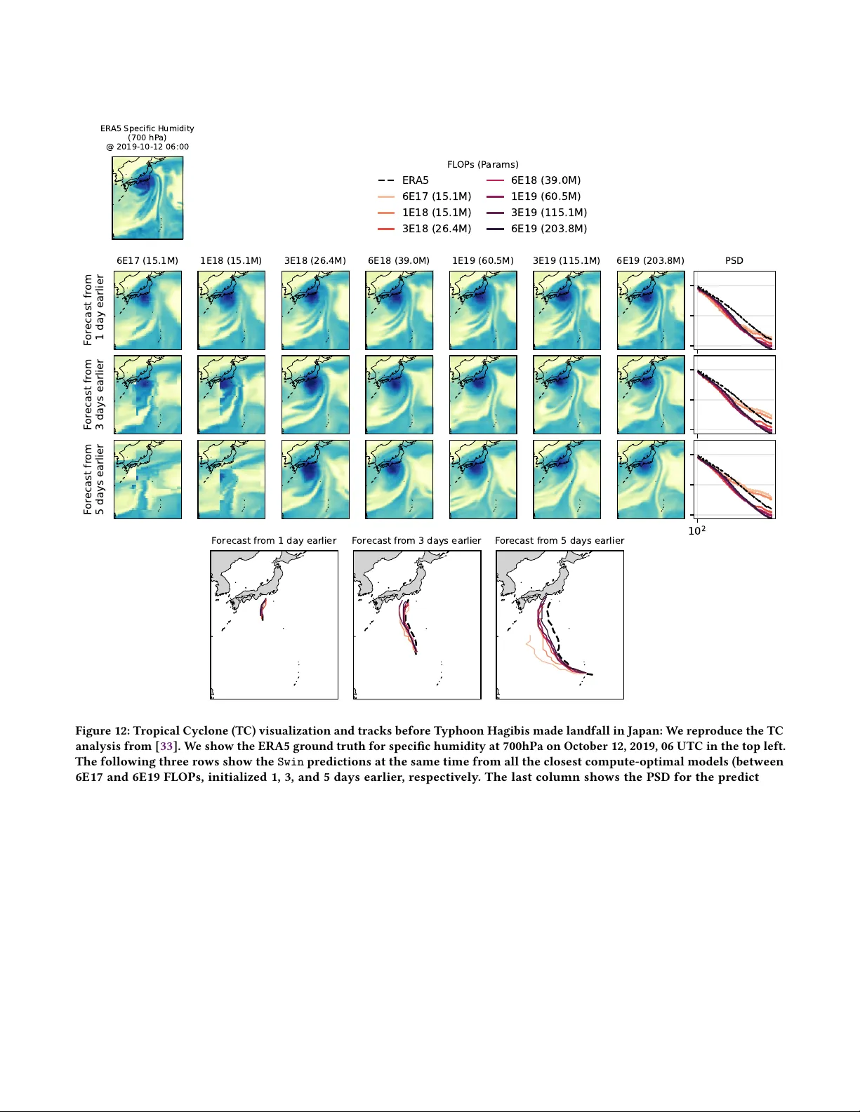
On Neural Scaling Laws for W eather Emulation through Continual T raining Shashank Subramanian shashanksubramanian@lbl.gov Lawrence Berkeley National Laboratory Alexander Kiefer kiefera@ornl.gov Oak Ridge National Laboratory Arnur Nigmetov anigmetov@lbl.gov Lawrence Berkeley National Laboratory Amir Gholami amirgh@berkeley .edu ICSI and UC Berkeley Dmitriy Morozov dmorozov@lbl.gov Lawrence Berkeley National Laboratory Michael W . Mahoney mmahoney@stat.berkeley .edu LBNL, ICSI, and UC Berkeley Abstract Neural scaling laws, which in some domains can pr edict the perfor- mance of large neural networks as a function of model, data, and compute scale, are the cornerstone of building foundation models in Natural Language Processing and Computer Vision. W e study neural scaling in Scientic Machine Learning, focusing on models for weather forecasting. T o analyze scaling b ehavior in as simple a setting as possible, we adopt a minimal, scalable, general-purpose Swin Transformer architecture, and we use continual training with constant learning rates and periodic cooldowns as an ecient train- ing strategy . W e show that models trained in this minimalist way follow predictable scaling trends and even outperform standard co- sine learning rate schedules. Co oldown phases can be re-purposed to improve downstream performance, e.g., enabling accurate multi- step rollouts over longer forecast horizons as well as sharper pre- dictions through spectral loss adjustments. W e also systematically explore a wide range of model and dataset sizes under various compute budgets to construct IsoFLOP curves, and we identify compute-optimal training regimes. Extrapolating these trends to larger scales highlights potential performance limits, demonstrating that neural scaling can ser ve as an important diagnostic for ecient resource allocation. W e open-source our code for repr oducibility . 1 Introduction Machine learning models, and deep learning models in particular , have demonstrated great success in scientic pr oblems, including emulating atmospheric physics for weather forecasting. In particu- lar , in recent years, several data-driv en models [ 3 , 6 – 8 , 10 , 27 , 33 ] have matched or surpassed the accuracy of gold-standard Numeri- cal W eather Prediction (NWP) systems that generate high-delity forecasts by solving complex, multiscale uid-dynamics equations. These data-driven models can generate weather forecasts orders of magnitude faster than classical N WP models using substantially lower resour ces, often only a single GP U, in infer ence. The training costs of these de ep learning weather emulators are rapidly increasing, as researchers explore a wide range of architec- tural choices, loss functions, and training methodologies in pursuit of state-of-the-art forecasting performance. These costs are further amplied by the growing scale of models, reaching 𝑂 ( 100 ) billion parameters, as well as increasing data resolutions, e.g., through smaller patch sizes in Transformer-based architectures [ 17 , 39 , 40 ]. Similar scaling challenges arise in areas such as Natural Language 1 0 5 1 0 6 #Samples 0.006 0.008 0.010 0.012 0.014 0.016 0.018 V alidation loss 1 epoch 5 epoch FL OP s 6E17 1E18 3E18 6E18 1E19 3E19 6E19 Optimal 100 200 300 400 P arameter count (M) Figure 1: Neural scaling for weather emulation. W e pre- train several models using continual training (constant learn- ing rates with periodic cooldowns; see § 3 ), and we identify compute-optimal r egimes to train the neural emulator so that neither data nor model size saturate at dierent com- pute budgets. At each FLOP budget, several mo del sizes (up to 400M) are trained to dierent dataset sizes to form IsoFLOPs that demonstrate the tradeo between model and data size. Unlike NLP mo dels, these systems are trained for multiple epochs (indicated by vertical dotted lines), causing samples to be revisited after the rst epoch and ee ctively be treated as pseudo-samples. W e t parab olas to each IsoFLOP, and we track the compute-optimal model at each budget. Processing (NLP) and Computer Vision (CV). Ho wever , scientic data present additional unique challenges, perhaps most notably their spatiotemporal structure. The proliferation of increasingly- complex architectures, in particular in Scientic Machine Learn- ing (SciML), raises important questions. Are we learning ab out weather for ecasting, or science more generally , or merely about the Shashank Subramanian, Alexander Kiefer, Arnur Nigmetov, Amir Gholami, Dmitriy Morozov, and Michael W . Mahoney idiosyncrasies of ever more elaborate (domain-motivated) neural architecture designs? What is the simplest possible architecture to obtain scaling that is good for downstream SciML applications? These questions are timely since, in many areas of machine learning, progress has ultimately been driven not by increased ar- chitecture complexity , but by scale—more data, larger models, and more compute—a phenomenon sometimes referred to as the bitter lesson . Understanding how performance scales with these quanti- ties therefore requires studying simple , general-purp ose models under controlled scaling regimes. Without such a foundation, it becomes dicult to disentangle genuine scaling behavior from artifacts introduced by specialized architectural choices. In domains such as NLP, this challenge has been addressed through the de velopment of neural scaling laws [ 20 , 21 , 23 ]. Distinct from other scaling concepts, such as strong scaling and weak scal- ing in high performance computing, neural scaling laws ar e a set of empirical patterns that guide practitioners in scaling data quan- tity , model size, and the amount of compute, so that none of them saturate. When this happens, the model loss follows a power-law relationship as a function of the size of the model, of the dataset, and of the computational resour ces available for training. Within NLP, these trends can span more than se ven orders of magnitude [ 16 , 21 ]. The study of neural scaling laws is important b ecause it builds condence and trust that model performance will improv e with increased scale. This predictive aspect is valuable because it makes neural scaling laws not only an analytical method but also actionable for planning ecient resource allocation. In the existing literature, there has been limited eort in under- standing the neural scaling behavior in SciML, in particular for deep learning models for weather forecasting. Existing studies do not explicitly investigate the joint relationship between model and data size, as a function of available computational budget, and/or their analyses remain incomplete. For example, Bodnar et al. [ 8 ] reports predictable scaling with model size; but it does not perform compute-optimal analyses, it relies on scaling with GP U time rather than FLOPs, and it incorp orates data outside the traditional weather- forecasting domain, such as pollutants and sea state, which makes interpreting the scaling behavior harder . In contrast, Karlbauer et al. [ 24 ] suggests that performance stalls, for neural op erators and related architectures, at ev en small model scales, although it should b e note d that this conclusion is drawn from experiments at coarser spatial resolution than we consider . More broadly , prior works stop short of identifying compute-optimal combinations of model size and data volume at each scale, making it dicult to disentangle true scaling laws from artifacts of architectural, data, or compute choices. In this work, we aim to systematically characterize the neural scaling relationships governing data-driven weather forecasting models. Our main contributions are: (1) Minimalist transformer architecture for neural scal- ing. Rather than designing specialize d architectures for weather forecasting, we intentionally adopt a minimalist and widely used backbone, the Swin Transformer [ 28 ], without domain-specic architectural modications or cus- tom loss functions, during pre-training. This design choice follows the principle that understanding scaling behavior requires reducing architectural confounders. Our goal is therefore not to engineer the most specialized weather model, but to understand how far simple architectures can be pushe d through scale. T o enable such experiments across a wide range of scales, we further implement 2 𝐷 spatial parallelism along with data parallelism, with the former being crucial for high resolution inputs. (2) Continual training for weather emulators. Inspired by Hägele et al. [ 22 ] , we apply learning rate (LR) cooldowns after a p eriod of continual training with a constant LR. Here, “ continual training” refers to the ability to continue optimizing a model across dierent compute budgets from a checkpoint without restarting fr om scratch, rather than the standard multi-task continual learning setting. W e show that this xed LR followed by a cooldown protocol can outperform the standard cosine schedule commonly used in pre-training weather emulators [ 8 , 27 ] (see Fig. 2 ). This approach enables ecient exploration of a wide range of compute budgets without retraining models from scratch, by periodically cooling down the LR to match the desired budget. W e show that e ven a cooldown period as short as 5% of the total training iterations is sucient to achiev e consistent performance (see Fig. 3 ). (3) Re-purposing cooldowns for better downstream per- formance. W e demonstrate that the short co oldown period can be re-purposed with alternate loss functions to better align the pre-trained model to downstream performance. For example, we can p erform multi-step r ollouts in training during cooldown to achieve higher accuracy over longer forecast horizons (see Fig. 3 , 4 ). W e may also spectrally ad- just the loss function (Fig. 4b ) to allow for sharper forecasts to capture critical high resolution features. Imp ortantly , this allows us to disentangle neural scaling from downstream performance, without which the scaling would be repeated for each loss function. (4) Neural scaling to identify compute-optimal training regimes. W e construct scaling laws by pre-training several models (up to 450 𝑀 parameters) using compute budgets from 6E+17 to 6E+19 FLOPs on the 0 . 25 ◦ ERA5 [ 19 ] dataset ( 𝑂 ( 300 , 000 ) samples at an hourly temporal resolution). For each budget, dierent models are cooled down to dierent iterations that give rise to IsoFLOP curves (see Fig. 1 , 5 ), a set of training congurations (model sizes and training iterations) that achieve a xed total training FLOPs. A cross these budgets, we obser ve clear compute-optimal scaling b e- havior , where each budget admits an optimal combination of model size and ee ctive dataset size. T o probe the limits of these trends, w e extrapolate the scaling laws to 2.25E+21 FLOPs and train a 1 . 3 B parameter model. This large-scale experiment shows signs of saturation before r eaching the projected loss. This suggests that scaling in this regime may become limite d by data size and spatiotemp oral resolution, highlighting the importance of neural scaling analyses for diagnosing when progress may require scaling data rather than model complexity . On Neural Scaling Laws for W eather Emulation through Continual Training 2 Related W orks Neural weather emulators. Models such as Four CastNet [ 26 ] approached the accuracy of NWP in medium-range weather fore- casting (10–14 days), while b eing orders of magnitude faster . New er models [ 7 , 8 , 10 , 27 , 33 ] hav e surpassed the accuracy of N WP, while retaining the speedups. The architecture landscape of these models includes Neural Operators[ 10 , 26 ], graph-based mo dels [ 27 , 33 ], and Transformer-based models [ 7 , 12 , 30 ]. Willard et al. [ 41 ] demon- strated that o-the-shelf Transformers that are trained well may be sucient for goo d performance. In addition to a variety of ar- chitectures, a variety of loss functions, including standard MSE, autoregressive rollout MSE [ 8 , 11 , 27 ], and sp ectral-based losses [ 36 ], have been employed, depending on the do wnstream objective. Despite this progress, with a focus on architectural design and ac- curacy , there has been relatively little eort in systematic analysis of how model design, data scale, and compute budget interact in weather emulators, which are central goals here . Neural scaling laws in large ML models. Research in other do- mains, most notably in NLP, has established the utility of neural scaling laws for guiding mo del development. Kaplan et al. [ 23 ] demonstrated that language model loss scales predictably as these axes incr ease, enabling researchers to estimate performance for larger models before training. Homann et al. [ 21 ] then formalized compute - optimal training (“Chinchilla” scaling), showing how to better balance model parameters and training data. More recent eorts have rened these laws, extended them to new architectur es, and explored their theoretical foundations [ 2 , 5 , 13 , 16 , 25 ]. Finally , Hägele et al. [ 22 ] show that LR scheduler changes that allow for continual training make the cost and design of neural scaling ex- periments more manageable. Our methodology is inspired by this. Neural scaling laws in large SciML models. There are also emerging eorts to apply scaling law concepts to SciML models, beyond NLP. For e xample, universal models of atomic systems have been developed with empirical scaling laws to guide capacity and data allocation across compute budgets, illustrating how scaling in- sights can transfer to scientic domains [ 38 , 42 ]. Another example in Nguyen et al. [ 29 ] builds foundation models that pr edict the func- tion and structure of biological sequences and discover the design space through neural scaling laws. Comprehensive neural scaling studies remain scarce in weather forecasting, and existing analyses mostly do not identify compute-optimal regimes and exhibit mixed ndings [ 8 , 24 ]. T oday , large models (with billions of parameters) [ 17 , 39 ] have already been trained for weather forecasting, further emphasizing the need to understand this design space. T o the best of our knowledge, the very recent work of Y u et al. [ 43 ] (which has appeared concurrent to this work) is the rst to consider neural scaling laws systematically for weather forecasting. In Y u et al. [ 43 ] , the authors scale up to 1E+18 FLOPs for existing models in the literature, and they demonstrate how some models show avors of compute optimal scaling, whilst others do not. The main dierences in our work is the emphasis on (i) continuous training with co oldowns for ecient neural scaling and down- stream alignment, (ii) scaling to over an order of magnitude higher compute (6E+19 FLOPs) via spatial parallelism to address memor y constraints, (iii) demonstrating compute-optimal regimes through a minimalist T ransformer backbone that matches state-of-the-art performance under the metrics of Rasp et al. [ 34 ] , and (iv) probing scaling limits under multi-epoch training by extending compute to O(2E+21) FLOPs. Our works aim to ll current gaps in scaling research by adapting neural scaling methodologies from NLP research to the context of data - driven weather emulation, providing systematic guidance for compute-optimal model design. 3 Overview of Methods Neural scaling involves pre-training a series of mo dels across a practical range of compute budgets. At each compute budget, sev- eral model sizes are trained to dierent numbers of data samples in order to remain on an IsoFLOP. The classical approach, based on the “Chinchilla” scaling laws [ 21 ], involves training models fr om scratch for each compute budget and model size. The need to train models from scratch is due to the reliance on the cosine LR sched- uler . Homann et al. [ 21 ] showed that the nal performance of any pre-trained model is optimal when the cosine LR decay length matches the total training duration. This LR scheduler is also popu- lar in other domains, including weather forecasting [ 8 , 26 ]. Several frontier NLP models as well as other SciML models have explored neural scaling laws in this manner [ 13 , 16 ]. Scaling with periodic cooldowns. While the above approach is popular , it is expensive. It would be more benecial to change the LR scheduler to a constant schedule, followed by a rapid cooldown phase to zero LR [ 22 ]. If one could show that the p erformance of this constant-plus-cooldown LR scheduler matches that of the cosine decay scheduler , then this would allow for training the series of models just once , considerably reducing the computational expense of neural scaling. W e record the loss at a given compute budget by applying a LR cooldown to zero in the nal pre-training iterations. T o reach larger budgets, we simply resume from the checkpoint prior to the cooldown, continue training with the original LR, and then cooldown at the next target budget. 3.1 W eather forecasting problem formulation Our goal is to model (emulate) global atmospheric dynamics using a learned neural network by predicting the temporal evolution of the state u ( x , 𝑡 ) , with x ∈ R 2 and 𝑡 ∈ [ 0 , ∞) . Our training dataset consists of discr ete snapshots u 𝑛 sampled at regular time steps with interval Δ 𝑡 with u 𝑛 ∈ R 𝐻 × 𝑊 × 𝐶 . Here, 𝐻 × 𝑊 is the height and width of the discretized latitude-longitude projection u ; 𝐶 is the number of state variables (as wind velocities, temperature, and others; see Appendix § A.2 , with vertical dimension treated as channels). The temporal evolution is modeled as: u 𝑛 + 1 = F 𝜃 ( u 𝑛 ) , (1) where F 𝜃 is a neural network parameterize d with weights 𝜃 . W e consider a standard mean-squared error ( MSE ) loss to pretrain F 𝜃 : L = min 𝜃  𝐵,𝐻 , 𝑊 , 𝐶 ( F 𝜃 ( u 𝑛 ) − ˆ u 𝑛 + 1 ) 2 , (2) with 𝐵 representing the batch size of samples and ˆ u is the target. Once traine d, the mo del produces forecasts during inference for 𝑁 steps, 𝑡 𝑛 + 𝑖 with 𝑖 ∈ { 1 , · · · , 𝑁 } , by autoregressively feeding each predicted state back as input to produce subsequent forecasts. Based Shashank Subramanian, Alexander Kiefer, Arnur Nigmetov, Amir Gholami, Dmitriy Morozov, and Michael W . Mahoney on prior work, w e consider two post-training strategies to better align the pre-trained model with the forecasting task: (1) Adjusted MSE ( AMSE ) : Pre-training datasets for weather con- tain time steps ( Δ 𝑡 ) that are undersampled; they ar e not ne enough to suciently resolve ne-scale atmospheric dynamics. With chaotic dynamics, this causes models traine d with MSE to smooth high-frequency structure. T o (partially) deal with this, we consider the adjusted MSE ( AMSE ) loss [ 36 ] (see Appendix § A.3 ), which disentangles decorrelation and spectral ampli- tude comp onents of the error , enabling the mo del to retain high-resolution features. (2) A utoregressive Rollouts ( AR ) : A utoregressive inference intro- duces generalization error due to a distribution shift, as pre- dicted states are use d as inputs instead of samples from the training distribution [ 11 ]. T o mitigate this, models are ne- tuned to autoregressively pr edict multiple time steps. While AR ne-tuning reduces forecast error over longer horizons, it often leads to overly smooth predictions due to the chaotic dynamics, causing models to b ehave like ensemble-mean fore- casts [ 33 ]. Existing approaches typically rely on heuristic schedules with multiple tunable components, including the number of autore- gressive steps, learning rate schedules, and ne-tuning duration, for both AR and AMSE strategies. In this work, we re-purpose the cooldown period to implement either strategy , aligning the model to the downstream task: maintaining high spectral resolution via AMSE , or reducing long-horizon forecast errors via AR. This approach re- moves the need for manually designed heuristic schedules. This also eliminates the need to experiment with these during pre-training, as they can be applied eciently after training. 3.2 Architecture and T raining W e employ a standard architecture based on the Shifted Window ( Swin ) Transformer [ 28 ]. While many weather models introduce domain-specic modications and customize d comp onents, we follow Willard et al. [ 41 ] , which demonstrates that standard trans- former backb ones can be highly competitive when trained well. Our input u 𝑛 is projected to the latent space X ∈ R 𝐻 / 𝑝 × 𝑊 / 𝑝 × 𝐸 using a standard patch emb edding layer with patch size 𝑝 and embed- ding dimensions 𝐸 . W e add a simple coordinate-based positional encoding using coordinates ( 𝑥 , 𝑦, 𝑧 ) (derived from spherical coordi- nates) and normalized time step 𝑡 ∈ R for each pixel, projected to the latent space P E ∈ R 𝐻 / 𝑝 × 𝑊 / 𝑝 × 𝐸 via an additional patch embed- ding layer . The positional encoding is added to the latent feature X before being passe d to the Swin Transformer blocks. While al- ternative positional encoding strategies exist, we av oid learnable encodings, which would introduce a large number of parameters at high input resolutions (especially for small patch sizes 𝑝 ) and risk over-parameterizing this component relative to the rest of the model. W e nd this positional encoding to be sucient in our experiments. For the Swin blocks, we r emove components such as relative p o- sitional bias and other non-essential modications, including the hi- erarchical Swin structure (e .g., patch merging and downsampling), and we retain a uniform Transformer block design consisting of windowed multi-head self-attention ( W -MHSA ) and a multi-layer perceptron (MLP) with pre-RMSNorm and residual connections: ˜ X = RMSNorm ( X ) , Y = W -MHSA ( ˜ X ) + X , ˜ Y = RMSNorm ( Y ) , O = MLP ( ˜ Y ) + Y , where the W -MHSA operation partitions the latent patch grid into 2 D windows and computes standard dot-product self-attention locally . W e use QK-normalization for training stability [ 18 , 44 ]. Every alternate block shifts the windows to enable cross-window interactions, implemented as a rolling operation with attention masks. W e modify the mask to preserve the left-right periodicity of the Earth system. The nal layer is a reverse patch embedding layer . Distributed training for neural scaling. As model, dataset, and input sizes increase, standard data parallelism becomes insucient, with per-GP U batch sizes dropping to one. While NLP models com- monly address this using model parallelism, SciML domains such as weather forecasting face dierent challenges. High-resolution inputs and small patch sizes make these models heavily constrained by intermediate activation memory rather than weights (and opti- mizer), a limitation that is further amplied during autoregressiv e rollout ( AR ) in training. Standard techniques such as Fully-Sharded Data Parallelism ( FSDP ) do little to alleviate this memory pressure. Moreover , I/O pressure incr eases due to high-resolution data. It is essential to build ecient distributed infrastructure to train across a wide range of scales. T owards this end, we implement spatial parallelism through do- main decomposition, along with data parallelism. W e employ a 2D array of 𝑛 1 × 𝑛 2 GP Us orthogonal to the data parallel GP Us ( 𝑛 𝑑 ), to further partition the input ( 𝐻 × 𝑊 ). Since activation memory scales as 𝑂 ( 𝐵 𝐻 𝑊 𝐸 ) , with batch size 𝐵 and embedding dimension 𝐸 , this partitioning eectively reduces this memory to 𝑂 ( 𝐵 𝐻 𝑊 𝐸 / 𝑛 𝑑 𝑛 1 𝑛 2 ) . The shifting window operation in the Swin require additional com- munication that we implement with a custom distributed rolling operation in the forward and backward pass (for details, se e Ap- pendix § A.3 ). 3.3 Empirical Analysis Setup Data. Our models are trained on the ERA5 [ 19 ] dataset that consists of around 350 , 000 samples of the Earth’s atmospheric state from 1979 to 2022 at an hourly temporal resolution and a spatial resolu- tion of 0 . 25 ◦ . While ERA5 consists of hundreds of state (physical) variables, we use a 71 variable subset following Willar d et al. [ 41 ] (see Appendix § A.2 ). When projected on a latitude-longitude grid, each sample is a 71 × 721 × 1440 tensor with 721 × 1440 representing the spatial grid. W e use the years 1979 to 2016 as training data, 2017 as validation, and 2020 for testing. W e train our models to predict a time step of 6 hours. Loss and Metrics. Our pre-training loss is MSE . W e avoid domain- specic weighting strategies that are variable dependent in the loss to maintain a simple objective for the neural scaling analysis. Our inputs are standardized mean and standard de viation derived per- variable from the training dataset. For validating our results, we use the area-weighted Ro ot Mean-Squared Error (RMSE) and Power Spectral Density (PSD) prediction and target for each variable. W e track each metric as a function of lead time up to 10 days, corre- sponding to the medium-range forecasting regime , and average the On Neural Scaling Laws for W eather Emulation through Continual Training 0 5000 10000 15000 20000 Iteration 0.0000 0.0001 0.0002 0.0003 0.0004 0.0005 L ear ning R ate (LR) LR Schedules W ar mup + Cosine W ar mup + Constant + Cooldown P eak LR = 5e-04 0 5000 10000 15000 20000 Iteration 0.008 0.01 0.02 0.03 0.04 V alidation L oss V alidation L oss vs Iterations Constant Cosine 6k Cosine 12k Cosine 18k Cosine 24k Cooldown 6k Cooldown 12k Cooldown 18k Cooldown 24k Figure 2: Loss behavior for cosine vs constant LR with cooldown. (left) LR schedules: The cosine sche dule follows a half-cosine decay after a xed warmup, while the constant + cooldown has a constant LR after the same xed warmup, but then cools down rapidly to 0 at the end. The cooldowns happen at the last 5% of iterations. (right) Loss vs iterations for dierent Swin models: The validation loss of the model continuously trained with a constant LR and cooled down to dierent iteration counts (here 5% of the total iteration is used as a cooldown period) shows b etter losses compared to the Swin trained from scratch with dierent cosine sche dulers that match the total iteration count. results over multiple initial conditions sampled across the evalua- tion period. W e follow this e valuation protocol on initial conditions sampled regularly for the testing year 2020 (every 12 hours, 732 initial conditions) based on Rasp et al. [ 34 ] . W e also retrieve the benchmark model predictions from Google Cloud Storage (using gcsfs ), following Rasp et al. [ 34 ] . While RMSE provides a measure of average error o ver the globe, the PSD is commonly used to assess the eective resolution of the predictions and to quantify how well high-frequency , ne-scale features ar e captured. Se e Appendix § A.2 for the denitions. Training. W e train all our models with a batch size of 16. Thr ough tuning experiments, we select a peak LR of 5E-4 for models larger than 100 𝑀 parameters. Similar to NLP [ 23 ], we nd smaller models can tolerate higher peak LRs, with the optimal LR scaling approxi- mately with the square root of the parameter count. W e train our models with the AdamW optimizer with a small weight decay of 1E-4 and gradient norms clippe d at 1 . W e nd that this, in con- junction with QK -normalization, is useful for training stability at the higher parameter counts. W e use the constant + cooldown LR scheduler of the scaling experiments and cosine for initial compar- isons. Both schedulers use 500 iterations as warmup. W e use mixed precision with float16 for training. See Appendix T ab. 1 for all hyperparameter choices. 4 Main Results W e demonstrate the following r esults: (R1) Neural weather models can be continuously traine d with periodic cooldowns using simple Transformer backb ones; (R2) Cooldown periods can be re-purpose d with alternate losses to align the T ransformer to a weather-specic downstream task; and (R3) Compute-optimal regimes, through systematic neural scaling using co oldowns, can b e identied for weather forecasting with scaling laws across multiple compute budgets. 0 .5 1 5 10 15 Cooldown fraction (%) 0.02 0.03 0.04 V alidation loss 6k 12k 18k 24k 6k- AR 12k- AR 18k- AR 24k- AR Figure 3: Loss as a function of total iterations used for cooldown. W e show the MSE over 36 hours (6 autoregressive steps) of prediction averaged over the validation data (2017). The MSE loss decreases predictably with longer cooldown du- rations and this is true over multistep predictions. At around 5%, the gains start to diminish. The loss behavior also holds when the cooldown is repurposed with 4-step AR loss that allows for lower errors across the longer horizon. (R1): Cosine vs. Cooldowns. W e show the two LR schedulers in Fig. 2 . W e rst train a moderately sized 115 𝑀 parameter Swin (see architecture hyp erparameters in Appendix T ab. 1 ) from scratch multiple times using the cosine LR schedule, each run to a dier- ent number of iterations ( batch size 16, corresponding to 20,819 iterations per epo ch). W e use the standard MSE loss with one-step prediction (predict the state Δ 𝑡 = 6 hours ahead). W e then replace this setup with the constant + cooldown LR schedule, cooling down to the same nal iteration counts as the cosine runs using only 5% of the total iterations. W e observe that the models that have been Shashank Subramanian, Alexander Kiefer, Arnur Nigmetov, Amir Gholami, Dmitriy Morozov, and Michael W . Mahoney 0 100 200 L ead T ime (hours) 1 2 3 4 RMSE u10m 0 100 200 L ead T ime (hours) 0.0005 0.0010 0.0015 0.0020 q700 0 100 200 L ead T ime (hours) 1 2 3 t850 0 100 200 L ead T ime (hours) 0 200 400 600 800 z500 Swin HRES GraphCast Swin- AR4 Swin- AMSE (a) RMSE of dierent variables (lab eled at the top) vs. lead time (in hours) for dierent models. 1 0 0 1 0 2 W avenumber 1 0 8 1 0 6 1 0 4 1 0 2 1 0 0 P ower Spectral Density u10m 1 0 0 1 0 2 W avenumber 1 0 1 2 1 0 1 0 1 0 7 1 0 5 q700 1 0 0 1 0 2 W avenumber 1 0 1 0 1 0 5 1 0 0 1 0 5 t850 1 0 0 1 0 2 W avenumber 1 0 5 1 0 0 1 0 5 1 0 1 0 z500 ER A5 Swin HRES GraphCast Swin- AR4 Swin- AMSE (b) PSD of dierent variables (labeled at the top) compared to PSD of the truth (ERA5) for dierent mo dels at 24 hours lead time. Figure 4: Cooldowns can be use d for alignment. When evaluated on testing year 2020, the Swin cooled down at 24000 iterations is able to surpass the N WP (HRES) and is comparable to the state-of-the-art deterministic deep learning benchmark, Graphcast. When AR is used in cooldown ( Swin - AR 4), the RMSE drops further , consistent with the use of this loss. When AMSE is used ( Swin - AMSE ), the PSD retains high wavenumbers. This is easily seen in 𝑞 700 where the AMSE spectra matches ERA5 p erfectly , but other models blur signicantly . AR contributes to more blurring in favor of reduced RMSE (visible in dissipation of power in high wavenumbers). W e note that HRES mo dels weather at a 0 . 1 ◦ resolution and hence shows higher resolution. cooled down consistently show lower validation loss compared to the cosine LR ( see Fig. 2 for the validation loss curves for each run). Hence, this is a valid (and better performing) strategy for continual training, to carry out cheaper neural scaling experiments. In order to use the cooldowns for neural scaling, we investigate what the optimal fraction of the total iterations should b e used for the cooldown period. W e repeat the cooldown experiments using dierent cooldown fractions (from 0% to 15%) for each nal itera- tion count. W e note that while the one-step prediction is important for training, the true utility of a neural emulator lies in its abil- ity to produce reliable forecasts over longer time horizons using autoregressive infer ence, as described in § 3 . Hence, we perform au- toregressive r ollouts during validation over multiple steps to track the time-averaged loss. Importantly , a co oldown that improves one- step loss but do es not translate to longer-horizon accuracy may reduce its practical benets. In Fig. 3 , we track the validation loss over six steps (36 hours), and we nd that the gains fr om cooldown translate to the downstream forecasting task as well. W e obser ve that even a small cooldown fraction (0.5%) is able to quickly reduce the loss and also see that a co oldown of 5% is sucient, beyond which the gains plateau. W e use 5% cooldowns in all experiments henceforth. (R2): Alignment with Co oldown. W e demonstrate that the cooldown can b e used to also align the mo del better with the down- stream task of high-resolution forecasting for several time steps. This is important be cause neural scaling can b e conducted using a simple MSE objective on large models and data, while the model’s be- havior can b e adapted during the co oldown (or post-training) using alternative objectives. As a result, scaling experiments need not be repeated each time the loss function is modied to improve perfor- mance on specic scientic tasks. W e consider both autoregressive training ( AR ) and the AMSE loss for this purp ose (as described in On Neural Scaling Laws for W eather Emulation through Continual Training 1 0 1 1 0 2 P arameter count (M) 0.006 0.008 0.010 0.012 0.014 0.016 0.018 V alidation loss FL OP s 6E17 1E18 3E18 6E18 1E19 3E19 6E19 Optimal 1 0 1 8 1 0 1 9 1 0 2 0 1 0 2 1 FL OP s 1 0 1 1 0 2 1 0 3 Optimal P arameter count (M) N = 2 . 2 2 5 2 e 0 4 × C 0 . 5 9 8 Compute optimal P r ojection: 1.32e+09 1B run: 1310M 1 0 1 8 1 0 1 9 1 0 2 0 1 0 2 1 FL OP s 1 0 2 Compute optimal L oss L = 1 . 2 3 e + 0 1 × C 0 . 1 6 8 Compute optimal P r ojection: L=0.0033 1B run: L=0.0053 Figure 5: Optimal model sizes as a function of compute. (left) Similar to Fig. 1 , we show the validation loss as a function of model size for dierent compute budgets. For each budget, the dierent model sizes are trained to a dierent number of iterations to create an IsoFLOP. W e track the minima for each IsoFLOP (through a tted parabola). (middle) W e t an empirical scaling law to nd the optimal mo del size for any FLOP budget and project to 2.25E+21 FLOPs to nd the optimal model. (right) W e also project the loss to the nal FLOP value—the measured loss at this FLOP value is saturated at 0.005. 0 100 200 L ead T ime (hours) 1 2 3 4 RMSE u10m 0 100 200 L ead T ime (hours) 0.0005 0.0010 0.0015 0.0020 q700 0 100 200 L ead T ime (hours) 1 2 3 t850 0 100 200 L ead T ime (hours) 0 200 400 600 800 z500 Swin- AR4 Swin- AR8 HRES GraphCast Figure 6: RMSE performance of compute-optimal Swin vs baselines. The 204M Swin (compute-optimal 6E+19 FLOPs) outp erforms NWP / HRES and is on-par with GraphCast when evaluated over initial conditions in 2020. The model is cooled down with 4 step AR . With more steps (8 step AR ), the performance gap reduces at longer lead times, as expecte d (GraphCast netunes with 2–12 step AR ). § 3 ). While AR aligns the model for long-term forecasting skill (by emulating an ensemble to produce smoother forecasts), AMSE aligns the models to produce high resolution features that are lost due to large timesteps. In Fig. 3 , we show that if the model is cooled down with 4-steps of AR , the validation loss systematically improves at all the iteration counts. In Fig. 4a , we show the RMSE of the Swin predictions as a function of lead time for several variables, compared to the NWP gold standard (HRES) [ 14 ] as well as the deterministic state-of-the- art emulator GraphCast [ 27 ]. W e see that the Swin is performant (outperforming HRES) and can be systematically pushed to the GraphCast accuracy through AR (note that GraphCast was ne- tuned with 1 through 12-step AR ). W e can also see from the PSD metric in Fig. 4b that the RMSE gains occur through smoothing that emulates an ensemble prediction. Similarly , using AMSE during cooldown, we see that RMSE remains largely unaected; however , the PSD plots show that the model has more power in the higher wavenumbers that this loss was designed to capture. W e emphasize that the goal here is not to achieve best possible performance, but rather to demonstrate that post-training phases such as cooldowns can be re-purposed to align model behavior in weather forecasting, highlighting their exibility without entangling them with the core scaling analysis. (R3): Neural Scaling. W e train a range of model sizes from 3 𝑀 to 456 𝑀 parameters (see all hyperparameters in Appendix T ab. 1 ), varying more than two orders of magnitude. W e select two orders of magnitude of compute budgets from 6E+17 to 6E+19. For each bud- get, we estimate (see Appendix § A.3 for details on FLOP estimates) a range of model sizes and number of iterations to train such that each conguration lies on an IsoFLOP. Each model is trained only Shashank Subramanian, Alexander Kiefer, Arnur Nigmetov, Amir Gholami, Dmitriy Morozov, and Michael W . Mahoney 0 100 200 L ead T ime (hours) 2 4 RMSE u10m 0 100 200 L ead T ime (hours) 0.0005 0.0010 0.0015 0.0020 q700 0 100 200 L ead T ime (hours) 1 2 3 4 t850 0 100 200 L ead T ime (hours) 0 200 400 600 800 z500 FL OP s (P arams) 6E17 (15.1M) 1E18 (15.1M) 3E18 (26.4M) 6E18 (39.0M) 1E19 (60.5M) 3E19 (115.1M) 6E19 (203.8M) Figure 7: RMSE performance of the closest compute-optimal Swin models at each compute budget. W e nd that RMSE at extended forecast horizons, up to 240 hours, consistently improves with increased compute. Howev er , at the highest compute levels, the rollout performance b egins to exhibit signs of saturation. 1 0 0 1 0 2 W avenumber 1 0 8 1 0 6 1 0 4 1 0 2 1 0 0 P ower Spectral Density u10m 1 0 0 1 0 2 W avenumber 1 0 1 2 1 0 1 0 1 0 7 1 0 5 q700 1 0 0 1 0 2 W avenumber 1 0 1 0 1 0 5 1 0 0 1 0 5 t850 1 0 0 1 0 2 W avenumber 1 0 5 1 0 0 1 0 5 1 0 1 0 z500 1 0 2 W avenumber 1 0 8 1 0 7 1 0 6 1 0 5 1 0 4 P ower Spectral Density u10m (k > 10²) 1 0 2 W avenumber 1 0 1 4 1 0 1 2 1 0 1 0 q700 (k > 10²) 1 0 2 W avenumber 1 0 1 0 1 0 8 1 0 6 1 0 4 t850 (k > 10²) 1 0 2 W avenumber 1 0 8 1 0 6 1 0 4 1 0 2 1 0 0 z500 (k > 10²) FL OP s (P arams) ER A5 6E17 (15.1M) 1E18 (15.1M) 3E18 (26.4M) 6E18 (39.0M) 1E19 (60.5M) 3E19 (115.1M) 6E19 (203.8M) Figure 8: PSD performance at lead time 24 hours of the closest compute-optimal Swin models at each compute budget. The PSD is evaluated at a 24-hour lead time and averaged over the test year . All mo dels accurately capture the low wavenumbers, while higher wavenumbers show gradual improvement as compute increases. The b ottom row zo oms in on the high-wavenumber range, where larger models exhibit sp e ctra that more closely match ERA5, whereas smaller models appear more blurred and display some articial high-wavenumber features. On Neural Scaling Laws for W eather Emulation through Continual Training once and cooled down to the required iteration at each IsoFLOP. W e note that sev eral of our models train for more than one epoch. In Fig. 1 , we show the IsoFLOP curves on the loss versus number of samples scaling plot, while Fig. 5 presents the corresponding scaling behavior of loss versus model size. For both plots, w e t parabolas to each IsoFLOP to estimate the compute-optimal dataset size and mo del capacity for a given budget. W e observe that (i) the model scales to 6E+19 plots without saturating the loss and (ii) exhibits compute-optimal behavior where each budget aor ds an optimal model size and sample count. Interestingly , this trend p er- sists even at 6E+19 where the model is trained for multiple epochs. In Fig. 6 , we show that the model that is closest to compute-optimal at 6E+19 FLOPs ( 204 𝑀 ) matches the state-of-the-art GraphCast (visualizations in Appendix Fig. 9 ). W e nd that the accuracy metrics maintain their gains through- out the rollout timesteps up to 240 hours and across dierent com- pute budgets. In Fig. 7 , we present the RMSE over the time horizon using the closest compute-optimal model at each budget. As the compute budget increases, accuracy improves not only for one-step predictions (as shown in the scaling results in Fig. 5 ) but also o ver longer time horizons. At the highest budgets, however , we start to see a saturation in accuracy for extended forecasts. In Fig. 8 , we visualize the PSD at a 24-hour lead time for all the above models. While all mo dels capture the lower wavenumbers accurately , we see that, with more compute, the models are able to capture the higher wavenumbers better . The smaller compute mo dels also exhibit arti- cial features at these wavenumbers (which is more pronounced in longer lead times, see Appendix Fig. 11 ) that becomes b etter with more compute. W e can also visualize this using a specic case study of a T ropical Cyclone (TC), see Appendix Fig. 12 , where the TC structures are sharper with the larger models. W e then derive the following scaling: 𝑆 ★ ( 𝐶 ) ∝ 𝐶 0 . 41 and 𝑁 ★ ( 𝐶 ) ∝ 𝐶 0 . 59 , where 𝐶 is the budget, 𝑆 ★ is the optimal number of (pseudo) samples (with the understanding that multiple epo chs are possible) and 𝑁 ★ is the optimal model size (see Fig. 5 ). W e extrapolate to 2.25E+21 FLOPs (more than an order of magnitude from the scaling analysis) to investigate how long the scaling holds. The empirical scaling suggests training a 1 . 3 𝐵 parameter mo del for 272 𝐾 itera- tions and we train this large model. W e obser ve in Fig. 5 that this model (denoted with star ) saturates b efore hitting the projected loss value. W e attribute this saturation to overtting as this mo del ne eds to be trained to more than 13 epo chs to reach this compute budget. W e show this in Appendix Fig. 13 by comparing the training and validation loss curves for all models. This provides early evidence that scaling trends may begin to break down in this regime, strongly motivating this kind of neural scaling analysis before moving SciML models to frontier model scales, data scales, and resolutions. 5 Conclusions W e systematically studied neural scaling for data-driven w eather forecasting SciML models. T o do so, we used a minimalist Trans- former backbone, without any domain-sp ecic complexities, so that scaling behavior could be studied in its simplest and most in- terpretable form, without confounding architecture / loss function choices. W e used a continual training approach with constant LRs and periodic cooldowns, an approach which oers several advan- tages. This outperforms the commonly-used cosine decay schedule; it enables rapid alignment of the mo del with downstream objec- tives during short cooldown phases; and, most importantly , it makes scaling law analysis practical by allowing IsoFLOP curves to be constructed without repeatedly training models from scratch. W e demonstrated this by eciently exploring a wide range of model sizes and compute budgets, identifying compute-optimal relation- ships between model size, dataset size, and training compute, with neural scaling trends emerging across two orders of magnitude in compute ( even with multi-epoch training). Our r esults indicate that extrapolating to very large compute budgets with models e xceeding a billion parameters shows signs of saturation. This may be due to the limited dataset size and the need to train for multiple epochs to reach these compute budgets. Even when following compute- optimal scaling, large models require multiple passes over the data, so simply increasing model size may not yield proportional gains. These observations suggest that very large SciML models should be carefully analyzed and planned before scaling further . Overall, our results emphasize that understanding neural scaling behavior for a given dataset is critical before training SciML models at fron- tier scale, and the y provide a practical frame work for doing so in spatiotemporal scientic domains. Acknowledgements This research used the Perlmutter supercomputing resources of the National Energy Research Scientic Computing Center (NERSC), a U.S. Department of Energy Oce of Science User Facility located at Lawrence Berkeley National Laborator y , operated under Con- tract No. DE- AC02-05CH11231. An award of computer time was provided by the ASCR Leadership Computing Challenge ( ALCC) program at NERSC under ERCAP0038267. SS would like to thank Ankur Mahesh for helpful discussions on weather mo deling and downstream metrics. Our conclusions do not necessarily reect the position or the policy of our sponsors, and no ocial endorsement should be inferred. References [1] Spherical harmonics: Power spectrum in signal processing. https://en.wikipedia. org/wiki/Spherical_harmonics#Power_spectrum_in_signal_processing . Wikipedia, The Free Encyclopedia. [2] Samira Abnar, Harshay Shah, Dan Busbridge, Alaaeldin Mohamed Elnouby Ali, Josh Susskind, and Vimal Thilak. Parameters vs ops: Scaling laws for optimal sparsity for mixture-of-experts language mo dels, 2025. URL https: //doi.org/10.48550/arXiv .2501.12370 . [3] Ferran Alet, Ilan Price, Andre w El-Kadi, Dominic Masters, Stratis Markou, T om R. Andersson, Jacklynn Stott, Remi Lam, Matthew Willson, Alvaro Sanchez- Gonzalez, and Peter Battaglia. Skillful joint probabilistic weather forecasting from marginals, 2025. URL https://ar xiv .org/abs/2506.10772 . [4] Mihai Alexe, Simon Lang, Mariana Clare , Martin Leutbecher , Christopher Roberts, Linus Magnusson, Matthew Chantry , Rilwan Adewoyin, Ana Prieto-Nemesio, Jesper Dramsch, Florian Pinault, and Baudouin Raoult. Data-driven ensemble forecasting with the aifs. ECMWF Newsletter , 181(Autumn 2024):32–37, 2024. doi: 10.21957/ma3p95hxe2. URL https://www.ecmwf.int/en/elibrary/81620- data- driven- ensemble- forecasting- aifs . [5] Y asaman Bahri, Ethan Dyer , Jared Kaplan, Jaehoon Lee, and Utkarsh Sharma. Explaining neural scaling laws. Proceedings of the National Academy of Sciences , 121(27), June 2024. ISSN 1091-6490. doi: 10.1073/pnas.2311878121. URL http: //dx.doi.org/10.1073/pnas.2311878121 . [6] Zied Ben-Bouallegue, Mariana CA Clare, Linus Magnusson, Estibaliz Gascon, Michael Maier-Gerber , Martin Janousek, Mark Rodwell, Florian Pinault, Jesper S Dramsch, Simon TK Lang, et al. The rise of data-driven weather forecasting. arXiv preprint arXiv:2307.10128 , 2023. URL https://doi.org/10.48550/arXiv .2307.10128 . Shashank Subramanian, Alexander Kiefer, Arnur Nigmetov, Amir Gholami, Dmitriy Morozov, and Michael W . Mahoney [7] Kaifeng Bi, Lingxi Xie, Hengheng Zhang, Xin Chen, Xiaotao Gu, and Qi Tian. Pangu-weather: A 3d high-resolution model for fast and accurate global weather forecast, 2022. URL https://doi.org/10.48550/arXiv .2211.02556 . [8] Cristian Bodnar , W essel P. Bruinsma, Ana Lucic, Megan Stanley , Anna V aughan, Johannes Brandstetter , Patrick Gar van, Maik Riechert, Jonathan A. W eyn, Haiyu Dong, Jayesh K. Gupta, Kit Thambiratnam, Alexander T . Archibald, Chun-Chieh Wu, Elizabeth Heider , Max W elling, Richard E. Turner , and Paris Perdikaris. A foundation model for the earth system, 2024. URL https://doi.org/10.48550/arXiv . 2405.13063 . [9] Boris Bonev , Thorsten Kurth, Christian Hundt, Jaideep Pathak, Maximilian Baust, Karthik Kashinath, and Anima Anandkumar . Spherical fourier neural operators: learning stable dynamics on the sphere, 2023. URL https://dl.acm.org/doi/10. 5555/3618408.3618525 . [10] Boris Bonev, Thorsten Kurth, Ankur Mahesh, Mauro Bisson, Jean K ossai, Karthik Kashinath, Anima Anandkumar , William D . Collins, Michael S. Pritchar d, and Alexander Keller . Fourcastnet 3: A geometric approach to probabilistic machine-learning weather forecasting at scale, 2025. URL https://doi.org/10. 48550/arXiv .2507.12144 . [11] Johannes Brandstetter , Daniel W orrall, and Max W elling. Message passing neural pde solvers, 2023. URL https://doi.org/10.48550/arXiv .2202.03376 . [12] Kang Chen, Tao Han, Junchao Gong, Lei Bai, Fenghua Ling, Jing-Jia Luo, Xi Chen, Leiming Ma, Tianning Zhang, Rui Su, Y uanzheng Ci, Bin Li, Xiaokang Yang, and W anli Ouyang. Fengwu: Pushing the skillful global medium-range weather forecast beyond 10 days lead, 2023. URL https://doi.org/10.48550/arXiv.2304. 02948 . [13] DeepSeek-AI, :, Xiao Bi, Deli Chen, Guanting Chen, Shanhuang Chen, et al. Deepseek llm: Scaling op en-source language models with longtermism, 2024. URL https://doi.org/10.48550/arXiv .2401.02954 . [14] European Centre for Medium-Range W eather Forecasts. Atmospheric mo del high resolution 10-day forecast ( set i - hres). https://w ww .ecmwf.int/ , 2023. April 5, 2024. [15] Facebook AI Research. fvcore: Collection of common code shared among fair computer vision projects. https://github.com/facebookresearch/fvcor e , 2023. Accessed: 2026-01-28. [16] Aaron Grattaori, Abhimanyu Dub ey , Abhinav Jauhri, Abhinav Pandey, Ab- hishek Kadian, Ahmad Al-Dahle, Aiesha Letman, Akhil Mathur, Alan Schelten, et al. The llama 3 herd of mo dels, 2024. URL https://doi.org/10.48550/arXiv.2407. 21783 . [17] Väinö Hatanpää, Eugene Ku, Jason Stock, Murali Emani, Sam Foreman, Chuny- ong Jung, Sandeep Madireddy , T ung Nguyen, V aruni Sastr y , Ray A. O. Sinurat, Sam Wheeler , Huihuo Zheng, Troy Arcomano, V enkatram Vishwanath, and Rao Kotamarthi. Aeris: Argonne earth systems model for reliable and skillful predictions, 2025. URL https://doi.org/10.48550/arXiv .2509.13523 . [18] Alex Henry , Prudhvi Raj Dachapally , Shubham Pawar , and Y uxuan Chen. Quer y- key normalization for transformers, 2020. URL https://doi.org/10.48550/arXiv . 2010.04245 . [19] Hans Hersbach, Bill Bell, Paul Berrisford, Shoji Hirahara, András Horányi, Joaquín Muñoz-Sabater, Julien Nicolas, Carole Peubey, Raluca Radu, Dinand Schepers, et al. The ERA5 global reanalysis. Quarterly Journal of the Royal Mete- orological Society , 146(730):1999–2049, 2020. URL https://doi.org/10.1002/qj.3803 . [20] Joel Hestness, Sharan Narang, Newsha Ardalani, Gregory Diamos, Heewoo Jun, Hassan Kianinejad, Md. Mostofa Ali Patwar y , Yang Y ang, and Y anqi Zhou. Deep learning scaling is predictable, empirically , 2017. URL https://doi.org/10.48550/ arXiv .2507.02119 . [21] Jordan Homann, Sebastian Borgeaud, Arthur Mensch, Elena Buchatskaya, Tre vor Cai, Eliza Rutherford, Diego de Las Casas, Lisa Anne Hendricks, Johannes W elbl, Aidan Clark, T om Hennigan, Eric Noland, Katie Millican, George van den Driessche, Bogdan Damoc, A urelia Guy, Simon Osindero , Kar en Simonyan, Erich Elsen, Jack W . Rae, Oriol Vinyals, and Laurent Sifre. Training compute-optimal large language models, 2022. URL https://doi.org/10.48550/arXiv .2203.15556 . [22] Alexander Hägele, Elie Bakouch, Atli K osson, Loubna Ben Allal, Leandro V on W erra, and Martin Jaggi. Scaling laws and compute-optimal training b eyond xed training durations, 2024. URL https://doi.org/10.48550/arXiv .2405.18392 . [23] Jared Kaplan, Sam McCandlish, T om Henighan, Tom B. Bro wn, Benjamin Chess, Rewon Child, Scott Gray , Alec Radford, Jerey Wu, and Dario Amodei. Scaling laws for neural language models, 2020. URL https://doi.org/10.48550/arXiv.2404. 14712 . [24] Matthias Karlbauer , Danielle C. Maddix, Abdul Fatir Ansari, Boran Han, Gaurav Gupta, Y uyang W ang, Andrew Stuart, and Michael W . Mahoney . Comparing and contrasting deep learning weather prediction backbones on navier-stokes and atmospheric dynamics, 2024. URL https://doi.org/10.48550/arXiv .2407.14129 . [25] Jakub Krajewski, Jan Ludziejewski, K amil Adamczewski, Maciej Piór o, Michał Krutul, Szymon Antoniak, Kamil Ciebiera, Krystian Król, T omasz Odrzygóźdź, Piotr Sankowski, Marek Cygan, and Sebastian Jaszczur . Scaling laws for ne- grained mixture of experts, 2024. URL https://doi.org/10.48550/arXiv.2402.07871 . [26] Thorsten Kurth, Shashank Subramanian, Peter Harrington, Jaideep Pathak, Morteza Mardani, David Hall, Andrea Miele, Karthik Kashinath, and Anima Anandkumar . Fourcastnet: Accelerating global high-resolution weather fore- casting using adaptive fourier neural operators. In Proceedings of the plat- form for advanced scientic computing conference , pages 1–11, 2023. URL https://dl.acm.org/doi/10.1145/3592979.3593412 . [27] Remi Lam, Alvaro Sanchez-Gonzalez, Matthew Willson, Peter Wirnsberger , Meire Fortunato, Ferran Alet, Suman Ravuri, Timo Ewalds, Leonard Casanova, Georey Tseng, et al. Learning skillful medium-range global weather forecasting. Science , 382(6677):1416–1421, 2023. URL https://doi.org/10.1126/science.adi2336 . [28] Ze Liu, Y utong Lin, Yue Cao , Han Hu, Yixuan W ei, Zheng Zhang, Stephen Lin, and Baining Guo. Swin transformer: Hierarchical vision transformer using shifted windows, 2021. URL https://doi.org/10.48550/arXiv .2103.14030 . [29] Eric Nguyen, Michael Poli, Matthew G. Durrant, Brian K ang, Dhruva Katrekar , David B. Li, Liam J. Bartie, Armin W . Thomas, Samuel H. King, Garyk Brixi, Jeremy Sullivan, Madelena Y . Ng, Ashley Lewis, Aaron Lou, Stefano Ermon, Stephen A. Baccus, Tina Hernandez-Boussard, Christopher Ré, Patrick D. Hsu, and Brian L. Hie. Sequence modeling and design from mole cular to genome scale with evo. Science , 386(6723):eado9336, 2024. doi: 10.1126/science.ado9336. URL https://www.science .org/doi/abs/10.1126/science.ado9336 . [30] T ung Nguyen, Rohan Shah, Hritik Bansal, Troy Arcomano, Romit Maulik, V eer- abhadra Kotamarthi, Ian Foster , Sande ep Madireddy , and Aditya Grover . Scaling transformer neural networks for skillful and reliable medium-range weather forecasting, 2024. URL https://doi.org/10.48550/arXiv .2312.03876 . [31] NVIDIA. Transformer engine: A librar y for accelerating transformer mo dels. GitHub repository . https://github.com/NVIDIA/TransformerEngine . [32] NVIDIA. Nvidia data loading librar y (dali), 2026. URL https://github.com/ NVIDIA/DALI . [33] Ilan Price, Alvaro Sanchez-Gonzalez, Ferran Alet, Timo Ewalds, Andrew El- Kadi, Jacklynn Stott, Shakir Mohamed, Peter Battaglia, Remi Lam, and Matthew Willson. Gencast: Diusion-base d ensemble forecasting for medium-range weather . arXiv preprint , 2023. URL https://doi.org/10.48550/ arXiv .2312.15796 . [34] Stephan Rasp, Stephan Hoyer , Alexander Merose, Ian Langmore, Peter Battaglia, T yler Russell, Alvaro Sanchez-Gonzalez, Vivian Y ang, Rob Carver , Shreya Agrawal, Matthew Chantry, Zied Ben Bouallegue, Peter Dueben, Carla Br omberg, Jared Sisk, Luke Barrington, Aaron Bell, and Fei Sha. W eatherbench 2: A bench- mark for the next generation of data-driven global weather models. Jour- nal of Advances in Modeling Earth Systems , 16(6):e2023MS004019, 2024. doi: https://doi.org/10.1029/2023MS004019. URL https://agupubs.onlinelibrary.wile y . com/doi/abs/10.1029/2023MS004019 . e2023MS004019 2023MS004019. [35] Mohammad Shoeybi, Mostofa Patwary , Raul Puri, Patrick LeGresley , Jared Casper , and Bryan Catanzaro. Megatron-lm: Training multi-billion parameter language models using model parallelism. arXiv preprint , 2019. URL https://doi.org/10.48550/arXiv .1909.08053 . [36] Christopher Subich, Syed Zahid Husain, Leo Separovic, and Jing Y ang. Fixing the double penalty in data-driven weather forecasting through a modied spherical harmonic loss function, 2025. URL https://doi.org/10.48550/arXiv .2501.19374 . [37] Paul A Ullrich, Colin M Zarzycki, Elizabeth E McClenny, Marielle C Pinheiro, Alyssa M Stanseld, and Kevin A Ree d. T empestextremes v2. 1: A commu- nity framework for feature detection, tracking, and analysis in large datasets. Geoscientic Model Development , 14(8):5023–5048, 2021. [38] Alexius W adell, Anoushka Bhutani, Victor Azumah, Austin R. Ellis-Mohr , Celia Kelly , Hancheng Zhao, Anuj K. Nayak, Kareem Hegazy , Alexander Brace, Hongyi Lin, Murali Emani, V enkatram Vishwanath, Kevin Gering, Melisa Alkan, T om Gibbs, Jack W ells, Lav R. Varshne y , Bharath Ramsundar, Karthik Du- raisamy , Michael W . Mahoney , Arvind Ramanathan, and V enkatasubramanian Viswanathan. Foundation models for discovery and exploration in chemical space, 2025. URL https://doi.org/10.48550/arXiv.2510.18900 . [39] Xiao W ang, Siyan Liu, Aristeidis Tsaris, Jong- Y oul Choi, Ashwin Aji, Ming Fan, W ei Zhang, Junqi Yin, Moetasim Ashfaq, Dan Lu, and Prasanna Balaprakash. Orbit: Oak ridge base foundation mo del for earth system predictability, 2024. URL https://doi.org/10.48550/arXiv .2404.14712 . [40] Xiao W ang, Jong-Y oul Choi, T akuya Kurihaya, Isaac Lyngaas, Hong-Jun Y oon, Xi Xiao, David Pugmire, Ming Fan, Nasik Muhammad Na, Aristeidis Tsaris, Ashwin M. Aji, Maliha Hossain, Mohamed W ahib, Dali W ang, Peter Thornton, Prasanna Balaprakash, Moetasim Ashfaq, and Dan Lu. Orbit-2: Scaling exascale vision foundation models for weather and climate downscaling. In Procee dings of the International Conference for High Performance Computing, Networking, Storage and Analysis , SC ’25, page 86–98, New Y ork, NY, USA, 2025. Association for Computing Machinery . ISBN 9798400714665. doi: 10.1145/3712285.3771989. URL https://doi.org/10.1145/3712285.3771989 . [41] Jared D. Willard, Peter Harrington, Shashank Subramanian, Ankur Mahesh, Travis A. O’Brien, and William D. Collins. Analyzing and exploring training recipes for large-scale transformer-based weather prediction, 2024. URL https: //doi.org/10.48550/arXiv .2404.19630 . [42] Brandon M. W ood, Misko Dzamba, Xiang Fu, Meng Gao, Muhammed Shuaibi, Luis Barroso-Luque, Kareem Abdelmaqsoud, V ahe Gharakhanyan, John R. Kitchin, Daniel S. Levine, K yle Michel, Anuroop Sriram, Taco Cohen, Abhishek Das, Ammar Rizvi, Sushree Jagriti Sahoo, Zachary W . Ulissi, and C. Lawrence On Neural Scaling Laws for W eather Emulation through Continual Training Zitnick. Uma: A family of universal models for atoms, 2025. URL https: //doi.org/10.48550/arXiv .2506.23971 . [43] Y uejiang Yu, Langwen Huang, Alexandru Calotoiu, and T orsten Hoeer . Scaling laws of global weather models. arXiv preprint , 2026. [44] Xiaohua Zhai, Alexander Kolesnikov , Neil Houlsby , and Lucas Beyer . Scaling vision transformers, 2022. URL https://doi.org/10.48550/arXiv .2106.04560 . Shashank Subramanian, Alexander Kiefer, Arnur Nigmetov, Amir Gholami, Dmitriy Morozov, and Michael W . Mahoney A Appendix : Additional Details A.1 Limitations The main limitation of this pap er is its focus on deterministic training of the weather model. Given the inherently chaotic nature of weather , probabilistic estimates are often more informative for forecasting at future time points, with metrics such as continuous ranked probability scores (CRPS) and spr ead-skill ratios (SSR) providing better diagnostics for a model’s predictive capability . Addr essing this would involve training (or cooling down) models using diusion objectives [ 4 , 33 ] or CRPS-based ensemble training [ 4 , 10 ], and this may exhibit dierent scaling behaviors—this is left for future work. Our patch size is xe d for the scaling tests, but the internal Transformer resolution (sequence length) represents another dimension for systematic scaling studies. Another possible limitation is the focus on T ransformer architectures. While this focus is intentional to demonstrate that simple architectures can scale and p erform competitively , it remains important to explore other architecture types, such as FourCastNet [ 10 ], which incorporates geometric inductive biases through spherical transforms within the neural operator framework, or graph-based approaches like GraphCast [ 27 ]. Finally , to rigorously probe the implications of scaling laws and not be constrained by multi-epoch training, it is essential to extend beyond this single domain, incorporating diverse datasets from across the Earth Sciences (and beyond), and exploring cross-domain foundation model pre-training. This will allow us to evaluate scaling b ehavior in a broader , more complex data landscape. A.2 ERA5 Dataset and Metrics For the current weather state 𝑢 𝑛 ∈ R 71 × 721 × 1440 , we closely follow existing works [ 10 , 41 ] and select the following variables: geopotential height ( 𝑧 ), winds ( 𝑢 , 𝑣 ), temperature ( 𝑡 ), and specic humidity ( 𝑞 ) at 13 vertical pressure levels ( 50 hPa, 100 hPa, 150 hPa, 200 hPa, 250 hPa, 300 hPa, 400 hPa, 500 hPa, 600 hPa, 700 hPa, 850 hPa, 925 hPa, and 1000 hPa). W e also include the following surface variables: 𝑢 10 𝑚 ( 𝑢 at 10 m), 𝑣 10 𝑚 ( 𝑣 at 10 m), 𝑡 2 𝑚 (temperature at 2 m), surface pressure ( 𝑠 𝑝 ), mean sea level pressure ( 𝑚𝑠𝑙 ), and total column water vap or ( 𝑡 𝑐 𝑤 𝑣 ). Finally , we include land-sea mask, orography , and cosine of the latitude (to convey the curvature of the earth) as static (not dependent on time) masks (not predicted). Our metrics are area-w eighted RMSE and PSD for each channel 𝐶 dened as follows. Given pr ediction 𝑢 𝑛 and ground truth ˆ 𝑢 𝑛 at time step 𝑛 , RMSE ( 𝑢 𝑛 , ˆ 𝑢 𝑛 ) = v u t 1 𝐻 𝑊 𝐻  ℎ = 1 𝑊  𝑤 = 1 𝑤 ℎ  𝑢 𝑐 ,ℎ,𝑤 − ˆ 𝑢 𝑐 ,ℎ,𝑤  2 , with 𝑤 ℎ being the area weights, proportional to the cosine of the latitude, normalized to one. The PSD [ 1 , 10 ] of 𝑢 at spherical harmonic degree ℓ is dened as: PSD ℓ ( 𝑢 ) = 1 2 ℓ + 1 ℓ  𝑚 = − ℓ | 𝑢 ℓ𝑚 | 2 , (3) where 𝑢 ℓ𝑚 are the coecients of 𝑢 in the spherical harmonic decomposition: 𝑢 ( 𝜃 , 𝜙 ) = ∞  ℓ = 0 ℓ  𝑚 = − ℓ 𝑢 ℓ𝑚 𝑌 ℓ𝑚 ( 𝜃 , 𝜙 ) , with 𝑌 ℓ𝑚 denoting the spherical harmonic functions of degree ℓ and order 𝑚 , and ( 𝜃 , 𝜙 ) the latitude and longitude coordinates. W e use torch-harmonics [ 9 ] to implement the Spherical Harmonic T ransform (SHT). W e apply all SHT s in FP64 to avoid numerical issues. W e use the SH T s for the metrics as well as the AMSE loss functions, dene d below . For the AMSE loss [ 36 ] between 𝑢 and ˆ 𝑢 , we have: AMSE ( 𝑢 , ˆ 𝑢 ) =  𝑘   PSD 𝑘 ( 𝑢 ) −  PSD 𝑘 ( ˆ 𝑢 )  2 + 2 max  PSD 𝑘 ( 𝑢 ) , PSD 𝑘 ( ˆ 𝑢 )   1 − Coh 𝑘 ( 𝑢, ˆ 𝑢 )  ! , (4) with the coherence between 𝑢 and ˆ 𝑢 at degree ℓ as: Coh ℓ ( 𝑢, ˆ 𝑢 ) = Í ℓ 𝑚 = − ℓ Re  𝑢 ℓ𝑚 ˆ 𝑢 ∗ ℓ𝑚   PSD ℓ ( 𝑢 ) PSD ℓ ( ˆ 𝑢 ) . (5) A.3 Model hyperparameters and training details W e train the Swin models (each with global batch size 16) summarized in T ab. 1 . W e nd that the small models can handle larger LRs and w e increase LRs for the smaller models up to 1 . 5 𝐸 − 3 . For the larger models, we decrease until 5 𝐸 − 4 . The LR (inversely) scales appro ximately with the square root of the parameter count in our tuning experiments. W e x our patch size to 4 based on previous studies patch size experiments [ 41 ]. However , we acknowledge that this is an additional moving part that we have not considered in this study . W e also x the head dimension to 64 through minimal hyp erparameter tuning experiments as well as the window size to 9 × 18 based on Willard et al. [ 41 ] . W e observe minimal accuracy gains with larger windows and smaller ones b egin to degrade the accuracy . For the feedfor ward (MLP) layers, On Neural Scaling Laws for W eather Emulation through Continual Training T able 1: Mo del congurations used for the neural scaling: W e run each of these models once to dierent nal iteration counts based on the required FLOP budgets with 5% cooldown periods at the end for the LR. Param (M) Embed Depth LR 3.1 192 6 1.5e-3 6.9 256 8 1.5e-3 15.1 384 8 1.5e-3 26.4 512 8 1.2e-3 39.0 512 12 1e-3 60.5 640 12 8e-4 86.8 768 12 6e-4 115.1 768 16 5e-4 153.5 1024 12 5e-4 203.8 1024 16 5e-4 304.5 1024 24 5e-4 456.7 1536 16 5e-4 we use a hidden size to embedding dimension ratio of 4 for all models. For the 1 . 3 𝐵 Swin , we use an embedding dimension of 1792 and depth 34 . For the cooldowns, we use a 1-sqrt() cooldown function based on Hägele et al. [ 22 ] . Given the high resolution ( 64800 = 180 × 360 sequence length from patch 4), we can only train most models with a local batch size of one. All our models are trained on NVIDIA A100 GP Us (40G memory capacity , unless specied). For models up to 100 𝑀 , we use only data parallelism (16 GP Us). For larger models, we emplo y various degrees of spatial parallelism using an orthogonal array of GP Us. For the largest model ( 456 . 7 𝑀 parameters) in neural scaling, we use 2 × 2 spatial parallel (4 GP Us) for a total of 64 GP Us. For AR cool downs with 4 steps, the memory complexity increases linearly and hence this model would then require 16 GP Us for spatial parallel and a total of 256 GP Us. For only the 1 . 3 𝐵 parameter model, we use 80G A100s and train it on 64 GP Us with spatial parallel 4 . Algorithm 1 Distributed Roll for Shifting Windows in Swin Require: Roll dimension 𝑑 , lo cal tensor 𝑥 (spatially sharded in 𝑑 across GP Us), shift size 𝑠 , spatial parallel GP U group G Ensure: T ensor 𝑥 rolled along dimension 𝑑 1: ( 𝑟 , 𝑃 ) ← rank _ and _ size ( G ) ⊲ GP U rank and world size 2: if 𝑃 = 1 or 𝑠 = 0 then 3: return roll ( 𝑥 , 𝑠 , 𝑑 ) ⊲ purely local case 4: right ← ( 𝑟 + 1 ) mod 𝑃 5: left ← ( 𝑟 − 1 ) mod 𝑃 ⊲ neighboring GP Us in the ring 6: if 𝑠 > 0 then 7: send ← 𝑥 [ . . . , − 𝑠 : , . . . ] ⊲ right boundar y slice 8: else 9: send ← 𝑥 [ . . . , : 𝑠, . . . ] ⊲ left boundar y slice 10: recv ← zeros _ like ( send ) ⊲ receive buer 11: distributed _ all _ to _ all _ single ( recv , send , G ) ⊲ 𝑠 > 0 sends right / receives left ⊲ 𝑠 < 0 vice versa 12: 𝑥 ← roll ( 𝑥 , 𝑠 , 𝑑 ) ⊲ local roll (b oundary will be correcte d) 13: if 𝑠 > 0 then 14: 𝑥 ← concat ( recv , 𝑥 [ . . . , − 𝑠 : , . . . ] , 𝑑 ) 15: else 16: 𝑥 ← concat ( 𝑥 [ . . . , : 𝑠 , . . . ] , recv , 𝑑 ) 17: return 𝑥 Hybrid spatial (domain) + data parallelism. The main ingredient in spatial parallelism is implementing a distributed roll operation. Instead of shifting the windows directly , the original Swin implementation [ 28 ] simply rolls (cylic-shifts) the image instead and applies an attention mask to limit the attention to each sub-windo w . When the image is partitioned across GPUs, this roll operation must happen acr oss the GP Us that shard the image. Hence, these spatial parallel GP Us must send and receive data from neighbors for an accurate roll. This boils down to a collective permute operation and we implement it using Py T orch’s torch.distributed.all_to_all_single collective. Following frontier NLP research codes from Megatron-LM [ 35 ], we implement the forward and backward pass of this distributed operation using Py T orch’s custom Autograd functions, where the backward pass is simply the conjugate forward operation: a reverse distributed roll. Shashank Subramanian, Alexander Kiefer, Arnur Nigmetov, Amir Gholami, Dmitriy Morozov, and Michael W . Mahoney ER A5 - u10m P r ed - u10m Er r or - u10m ER A5 - q700 P r ed - q700 Er r or - q700 ER A5 - t850 P r ed - t850 Er r or - t850 ER A5 - z500 P r ed - z500 Er r or - z500 15 10 5 0 5 10 15 20 15 10 5 0 5 10 15 20 10 5 0 5 10 0.000 0.002 0.004 0.006 0.008 0.010 0.000 0.002 0.004 0.006 0.008 0.010 0.006 0.004 0.002 0.000 0.002 0.004 0.006 240 250 260 270 280 290 300 240 250 260 270 280 290 300 8 6 4 2 0 2 4 6 8 46000 48000 50000 52000 54000 56000 58000 46000 48000 50000 52000 54000 56000 58000 400 300 200 100 0 100 200 300 400 Figure 9: Predictions from the 204M parameter model: W e show the ground truth ERA5, the prediction, and the error in physical units for four variables. The predicted forecasts also qualitatively match the ground truth. W e show the distributed roll algorithm in Alg. 1 . W e note that this is not a full replacement for distributed torch.roll , as we assume we only need to send one slice to one neighboring GP U and receive one slice from another neighb oring GP U. This is true for Swin , because we shift by a half of the window size, and windows are not sharded across GP Us in our setting (there is at least one window on every GP U). For brevity , we also omit the permute operations to bring the shift dimension to position 0 and back ( all_to_all_single only acts on the rst dimension). Finally , spatial parallel introduces weights (and bias) tensors that ar e shared across the spatial parallel GPU groups (in addition to the data parallel GP Us that, by design, share the model weights). Hence, the weight gradients ( wgrads ) must be additionally reduced in this group (along with the data parallel group). Our simplistic Swin model design (with coordinate position embeddings) leads to all the weights (and bias) tensors shared across the spatial parallel group and hence we implement this as a joint AllReduce operation across the combined data and spatial parallel GP U group using a communication ho ok in PyT orch’s DistributedDataParallel . W e verify with Unit T ests that the distributed forward and backward passes (including weight gradients and adjoints) match the non-distributed version ensuring accuracy of our custom model parallelism. Finally , we also use NVIDIA TransformerEngine [ 31 ] for easy access to fused operations and support for 4D parallelism with tensor parallelism. While we do not use tensor parallelism in any run, we note that the code supports this parallelism as well for scaling up. Here, an additional orthogonal array of GP Us may be employ ed to further shar d the model weights ( similar to NLP). TransformerEngine provides a drop-in replacement for Linear layers in our model to use tensor parallelism. W e note that some bias tensors may be shared across tensor and spatial parallel GP U groups with this additional parallelism and we take care of this through On Neural Scaling Laws for W eather Emulation through Continual Training custom communication hooks in DistributedDataParallel . Unit tests conrm that combined spatial, tensor , and data parallelism yeild the correct distributed forward pass outputs and backward pass wgrads and dgrads . Ecient and stateful dataloaders. Our data is stored in HDF5 les, with one le per year of ERA5, to eciently leverage the Lustre lesystem in our experiments for high-throughput data access. W e use NVIDIA DALI [ 32 ] dataloaders, which automatically overlap data loading with computation during the forward and backward passes and perform pre-processing operations, such as data normalization, directly on the GP U. This ensures that data I/O does not become a performance bottleneck. Finally , we train our models to xed iteration counts (to support periodic cooldowns under a predene d FLOP budget), which requires checkpoint–restart functionality to operate correctly mid-epoch. T o enable this, we implement stateful dataloaders within D ALI that track both the shued sample indices and the number of completed iterations, allowing training to resume seamlessly from arbitrary mid-epoch checkpoints. Code. W e open-source our code at https://github.com/ShashankSubramanian/neural- scaling- weather . For all our FLOP computations, due to the homogeneous design of the Swin , we use standard analytical attention and MLP FLOP estimates, taking into account the windowed attention, and verify with fvcore [ 15 ] that our analytical values are close to the correct estimates. W e include the patch, p osition, and reverse-patch embedding FLOPs as well in our estimation. The FLOP expr essions can be found in utils/flops_utils.py in our code. A.4 Additional results W e visualize the prediction from the compute-optimal model ( 203 . 8 𝑀 ) at the large budget 6E+19 in Fig. 9 , along with the bias (error) between the predictions and the ground truth (ERA5). The predictions are obtained on the testing year 2020, with initial conditions e very 12 hours (for a total of 732 initial conditions). Bey ond the quantitative metrics dened earlier , w e observe that the model produces r ealistic predictions of the physical elds, capturing the main spatial structures and patterns present in the refer ence data. All the Swin models t on a single GP U ( A100 40G) during inference. Most mo dels generate 10 day forecasts in less than a minute (including metric computations). For example, the 204 𝑀 Swin takes 32 seconds, while the largest 1 . 3 𝐵 Swin takes around 96 seconds to generate the same 10 day forecast. These models preserve the emulator’s substantial computational advantage over the NWP, achieving a speedup of more than 100 × [ 4 ]. In Fig. 10 , we show the PSD of dier ent variables for two lead times (1 day and 5 days). The Swin model cooled down with AR 4 loses a signicant amount of energy at small scales, resulting in overly dissipated forecasts and an eective resolution much coarser than what the 0 . 25 ◦ grid can support. In contrast, the Swin model cooled down with AMSE matches the PSD of the gr ound truth almost exactly at short lead times. At longer lead times, it exhibits higher energy than the gr ound truth at the smallest scales suggesting a noise-driven eective resolution that exceeds that of the dissipated AR 4 forecasts, as noted in Subich et al. [ 36 ] . Overall, the two cooling strategies guide the model toward dierent objectives: one prioritizes lo wer overall RMSE ( and skill) over long lead times, akin to ensemble for ecasting, while the other emphasizes high realism, preserving small-scale features in the forecast. In Fig. 8 and Fig. 11 , we show the PSD for the closest compute-optimal model at each compute budget for a 24-hour and 120-hour lead time. While all models faithfully captur e the PSD at the lower wavenumbers, the higher compute models show b etter PSD at the higher wavenumbers as well, better capturing the sharper features. Howev er , improvements with increasing compute are gradual and sho w signs of saturation. Additionally , low er-compute models exhibit articial power at high wavenumbers, which becomes mor e pronounced at longer lead times (120 hours). In contrast, higher-compute models maintain more consistent performance across lead times. These spectral improvements are more visible in a specic physical case study . Se e Fig. 12 . W e reproduce the study that analyzes the Tr opical Cyclone (TC) patterns of T yphoon Hagibis from [ 33 ]. W e use the same TC tools as the study— T empestExtremes [ 37 ], in order to visualize TC tracks. Here, w e track the TC structure across the compute-optimal models initialized at 1, 3, and 5 days from the TC landfall time on October 12, 2019, 06 U TC. W e visualize the specic humidity at 700hPa for all the forecasts as well as the PSD (compared to ERA5). For short forecasts (1 day), all models are faithful with increased compute resulting in sharper predictions (also quantied in the PSD). With longer forecasts (3 and 5 days earlier), the smaller models exhibit articial features (patch artifacts, discontinuities in the prediction) that is also seen in the sp ectral power at the high wavenumbers. With more compute, the models b egin to produce realistic TCs at these lead times as well. W e also visualize the TC tracks. While all models follo w the general track of ERA5, the smaller models show more variability at longer lead times due to artifacts developing. W e note that, due to the deterministic modeling framework, these results should be interpreted as illustrative. A ccurately tracking such phenomena, particularly at longer lead times, requires pr obabilistic (ensemble) forecasting, as the chaotic nature of atmospheric processes naturally introduces more spread ( variance) in the predictions, particularly at longer lead times. Finally , in our extrapolated scaling to 1 . 3 𝐵 parameters, we observe a saturation of performance as se en in Fig. 5 . This is attributed to around 13 epochs of training and hence high chances of ov ertting with the large ( high parameter count) model. W e show this in Fig. 13 where for all the models in the scaling regime (6E+17 to 6E+19) the training and validation loss track closely . Howev er , for the model extrapolated to 2.25E+21 FLOPs, while the training loss reaches close to the extrapolate d loss value of 0 . 033 , the validation loss plateaus at around 0 . 053 , pointing to signicant overtting. Although the validation loss continues to improve slightly with more compute, the growing gap suggests increased memorization of training data, which may reduce generalization abilities as well. Shashank Subramanian, Alexander Kiefer, Arnur Nigmetov, Amir Gholami, Dmitriy Morozov, and Michael W . Mahoney 1 0 0 1 0 2 W avenumber 1 0 8 1 0 6 1 0 4 1 0 2 1 0 0 P ower Spectral Density u10m 1 0 0 1 0 2 W avenumber 1 0 1 2 1 0 1 0 1 0 7 1 0 5 q700 1 0 0 1 0 2 W avenumber 1 0 1 0 1 0 5 1 0 0 1 0 5 t850 1 0 0 1 0 2 W avenumber 1 0 5 1 0 0 1 0 5 1 0 1 0 z500 ER A5 Swin HRES GraphCast Swin- AR4 Swin- AMSE (a) PSD of dierent variables compared to PSD of the truth (ERA5) for dierent mo dels at 24 hours lead time. 1 0 0 1 0 2 W avenumber 1 0 8 1 0 6 1 0 4 1 0 2 1 0 0 P ower Spectral Density u10m 1 0 0 1 0 2 W avenumber 1 0 1 5 1 0 1 2 1 0 1 0 1 0 7 1 0 5 q700 1 0 0 1 0 2 W avenumber 1 0 1 0 1 0 5 1 0 0 1 0 5 t850 1 0 0 1 0 2 W avenumber 1 0 5 1 0 0 1 0 5 1 0 1 0 z500 ER A5 Swin HRES GraphCast Swin- AR4 Swin- AMSE (b) PSD of dierent variables compared to PSD of the truth (ERA5) for dierent models at 120 hours lead time. Figure 10: PSD of predictions at 1 day and 5 days: While AR produces blurrier forecasts (though with lower RMSE), AMSE helps retain p ower at high wavenumbers. At longer lead times, such as 120 hours, Swin - AMSE continues to show signicant power at these small scales. This allows practitioners to dene an eective resolution based on this noise-level as outline d in Subich et al. [ 36 ]. On Neural Scaling Laws for W eather Emulation through Continual Training 1 0 0 1 0 2 W avenumber 1 0 6 1 0 4 1 0 2 1 0 0 P ower Spectral Density u10m 1 0 0 1 0 2 W avenumber 1 0 1 2 1 0 1 0 1 0 7 1 0 5 q700 1 0 0 1 0 2 W avenumber 1 0 1 0 1 0 5 1 0 0 1 0 5 t850 1 0 0 1 0 2 W avenumber 1 0 5 1 0 0 1 0 5 1 0 1 0 z500 1 0 2 W avenumber 1 0 7 1 0 6 1 0 5 1 0 4 P ower Spectral Density u10m (k > 10²) 1 0 2 W avenumber 1 0 1 4 1 0 1 2 1 0 1 0 q700 (k > 10²) 1 0 2 W avenumber 1 0 1 0 1 0 8 1 0 6 1 0 4 t850 (k > 10²) 1 0 2 W avenumber 1 0 8 1 0 6 1 0 4 1 0 2 1 0 0 z500 (k > 10²) FL OP s (P arams) ER A5 6E17 (15.1M) 1E18 (15.1M) 3E18 (26.4M) 6E18 (39.0M) 1E19 (60.5M) 3E19 (115.1M) 6E19 (203.8M) Figure 11: PSD performance at lead time 120 hours of the closest compute-optimal Swin models at each compute budget: The PSD is evaluated at a 120-hour lead time and averaged over the test year . All models accurately capture the low wavenumbers, while higher wavenumbers show gradual improvement as compute increases. The b ottom row zo oms in on the high-wavenumber range, where larger models exhibit sp e ctra that more closely match ERA5, whereas smaller models appear more blurred and display some articial high-wavenumber features. These features are more dominant at this longer lead time compared to 24 hours in Fig. 8 . Shashank Subramanian, Alexander Kiefer, Arnur Nigmetov, Amir Gholami, Dmitriy Morozov, and Michael W . Mahoney ER A5 Specific Humidity (700 hP a) @ 2019-10-12 06:00 FL OP s (P arams) ER A5 6E17 (15.1M) 1E18 (15.1M) 3E18 (26.4M) 6E18 (39.0M) 1E19 (60.5M) 3E19 (115.1M) 6E19 (203.8M) 6E17 (15.1M) 1E18 (15.1M) 3E18 (26.4M) 6E18 (39.0M) 1E19 (60.5M) 3E19 (115.1M) 6E19 (203.8M) PSD 1 0 2 F or ecast fr om 1 day earlier F or ecast fr om 3 days earlier F or ecast fr om 5 days earlier F or ecast fr om 1 day earlier F or ecast fr om 3 days earlier F or ecast fr om 5 days earlier Figure 12: Tropical Cyclone (TC) visualization and tracks before T ypho on Hagibis made landfall in Japan: W e reproduce the TC analysis from [ 33 ]. W e show the ERA5 ground truth for specic humidity at 700hPa on October 12, 2019, 06 U TC in the top left. The following three rows show the Swin predictions at the same time from all the closest compute-optimal models ( between 6E17 and 6E19 FLOPs, initialized 1, 3, and 5 days earlier , respectively . The last column sho ws the PSD for the predictions (zoomed into the high wavenumbers). Forecasts initialized 1 day earlier show that all models capture the TC structure, although the larger models produce systematically sharper features, which is also reected in the PSD . For initializations 3 and 5 days earlier , the smaller models fail to capture the TC structure, exhibiting patching artifacts and generally inconsistent blending of physical features. This b ehavior is likewise evident in the PSD as articial high-wavenumber energy . In contrast, the larger models consistently capture the TC across all lead times. The last row shows the TC track from the dierent initializations. Although a deterministic mo del is insucient for accurately assessing track performance, some variability among the dierent models is seen. On Neural Scaling Laws for W eather Emulation through Continual Training 0 50000 100000 150000 200000 250000 Iteration 1 0 2 T rain L oss V al L oss P arams 15.1M 26.4M 39.0M 60.5M 115.1M 203.8M 1.3B Figure 13: Training and validation loss as a function of iterations for dierent models: W e show the training curves for all the (closest) compute-optimal mo dels. All losses were logged at a frequency of 2000 iterations except the 1.3B model that was logged at a frequency of 10,000 iterations. The training and validation loss cur ves track each other closely . However , for the 1.3B model, we observe signicant overtting.