Anchored-Branched Steady-state WInd Flow Transformer (AB-SWIFT): a metamodel for 3D atmospheric flow in urban environments

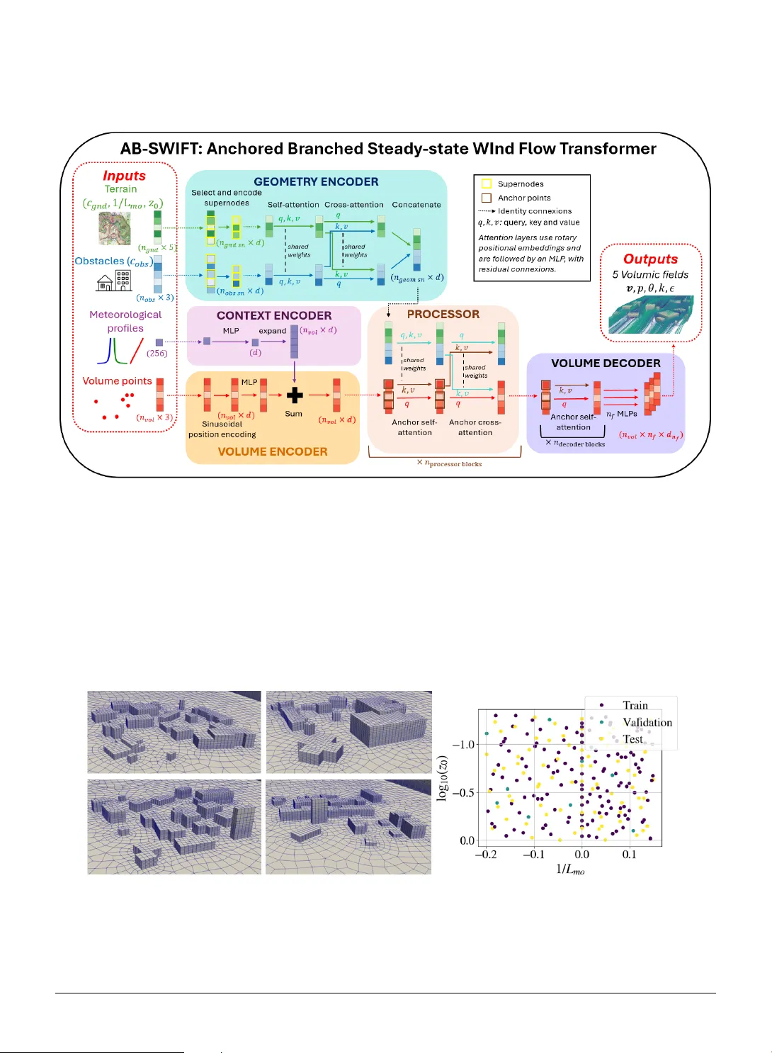
Anc hored-Branc hed Steady -s tate WInd Flow T r ansf or mer (AB-S WIFT): a metamodel f or 3D atmospher ic flo w in urban en vironments Armand de V illeroché a , ∗ , Rem–Sophia Mouradi a,c , Vincent Le Guen b,c , Sibo Cheng a , Marc Bocquet a , Alban Farchi a , Patrick Ar mand d and Patrick Massin a a CEREA, ENPC, EDF R&D, Institut P olytec hnique de Paris, Île-de-F rance, F rance b SINCL AIR AI Laboratory, Saclay, Île-de-F rance, Fr ance c EDF R&D, Île-de-F rance, F rance d CEA, DAM, DIF , F-91297 Arpajon, Fr ance A R T I C L E I N F O Keyw ords : Computational fluid dynamics Deep lear ning Geometric deep learning Transf ormers Atmospheric dispersion Atmospheric stratification stability Atmospheric boundar y layer A B S T R A C T Air flow modeling at a local scale is essential for applications such as pollutant dispersion modeling or wind farm modeling. To circumv ent costl y Computational Fluid Dynamics (CFD) computations, deep lear ning sur rogate models hav e recently emerged as promising alter nativ es. How ever , in the context of urban air flow , deep lear ning models str uggle to adapt to the high variations of the urban geometry and to larg e mesh sizes. To tackle these challenges, we introduce Anchored Branched Steady-state WInd Flow Transf ormer (AB-SWIFT), a transformer-based model with an internal branched structure uniquely designed for atmospheric flow modeling. W e train our model on a specially designed dat abase of atmospheric simulations around randomised urban geometries and with a mixture of unstable, neutral, and stable atmospheric stratifications. Our model reaches the best accuracy on all predicted fields compared to state-of-t he-art transf ormers and graph-based models. Our code and data is a vailable at https://github.com/cerea- daml/abswift. 1. Introduction Microscale modeling of the atmospheric flow is important for sev eral applications. Ho wev er, some applications ma y require a large number of simulations, such as design optimization of wind farm performances ( Ivanell et al. , 2025 ), long-term plant g ro wth under solar panels ( Joseph et al. , 2025 ), or real-time modeling and solving in verse problems, such as pollutant dispersion ( T ognet , 2015 ). While Computational Fluid Dynamics (CFD) can be used to model t he atmospheric flo w ov er complex urban areas ( code_satur ne , 2025 ), CFD simulations can be slow and expensiv e when high mesh refinement is necessary . This makes them cumbersome when many simulations or fas t responses are needed. Machine learning has recently gained attraction as a viable option to dev elop f ast sur rogates ( Kar niadakis et al. , 2021 ). Ho wev er, local air flow s present sev eral complex challeng es f or machine lear ning sur rogates. Firstl y , f or urban areas, the geometry may represent an y building shapes and lay outs, which can v ar y significantly . Secondly , deep learning approaches tend to str uggle to scale to large meshes required by real-case scenarios. Finally , flow behavior in the atmospheric boundary lay er is influenced by atmospher ic stratification stability , which modifies the turbulence lev el in the flow and must be taken into account ( Hanna et al. , 1982 ). T o tackle t hese challenges, we propose Anchored-Branched Steady -state WInd Flow Transf or mer (AB-SWIFT), a model designed f or atmospheric flow modeling. Our model includes an inter nal branched s tructure adapted to the multiple components of microscale atmospher ic simulations. This allows to flexibl y and expressiv ely take into account terrain topology as well as complex obst acles affecting t he flow . Our model also takes as inputs vertical meteorological profiles, an important dr iver of t he simulations. This option enables v ar ious flow conditions, suc h as atmospheric stratification st ability , with a higher number of degrees of freedom, without being restrained to a specific parameterization of the meteorology . Our main contributions are as f ollows: ∗ Corresponding author armand.de-villeroche@edf.fr (A.d. Villeroc hé) OR CID (s): 0009-0001-8811-7443 (A.d. Villeroché) A. d. Villero ché et. al: Pr epr int submitted to Elsevier Page 1 of 17 Ancho red-Branched Steady-state WInd Flo w T ransformer • W e present AB-SWIFT, t he first transf or mer based neural operator dedicated to atmospher ic flow s at a local scale. • W e train our model with a new dat aset of atmospher ic flow s in urban areas wit h different building la youts on flat terrain. Our dat aset is also the first to include various atmospheric stratification stabilities. • Our model achie ves the best accuracy relativ e to state-of-the-ar t T ransf or mers and Graph Neural Networ k s baselines. • Our code and data are a vailable at https://github.com/cerea-daml/abswift. 1.1. Related w orks Neur al operat ors Deep lear ning models hav e recentl y gained traction as surrogate models of phy sical sys tems. In particular, data-dr iven neural sur rogates attempt to lear n from dat a the solution operator  𝑆 that maps inputs 𝐴 to outputs 𝑈 ( Cheng et al. , 2025 ). For instance, in a time-independent setting, 𝐴 can represent simulation parameters and geometry , and 𝑈 can represent 3D stationar y v olumic fields or integrated scalar quantities. Neural operators ( Kov achki et al. , 2023 ) attempt to learn directly in the function space, where 𝐴 and 𝑈 represent continuous functions. In practice, only access discretized representations of 𝐴 and 𝑈 are a vailable. A ke y requirement to define a neural operator is t hen the independence to the discretization sc heme of 𝐴 and 𝑈 and con verg ence with t he discretization resolution. Most sur rogate models, including ours, f ollow t he encode-process-decode scheme. This approach decomposes  𝑆 into an encoder  𝐸 , a processor  𝑃 , and a decoder  𝐷 so t hat:  𝑆 =  𝐷 ◦  𝑃 ◦  𝐸 . The encoder transforms phy sical inputs into latent tokens , i.e. scalar -valued v ectors of a fixed dimension. The processor can t hen operate in the dimensional space of t he latent tok ens, called the latent space , and is usually designed to car ry the major ity of the comput ational burden. Finall y , the decoder maps tokens back into the ph ysical space to predict the desired quantities of interest. Deep learning surr og ates for urban atmospheric flo w Sev eral past contributions f ocus on modeling 3D atmospheric flow in built-up en vironments. Villeroché et al. ( 2026 ) use a Multi-La yer Perceptron (MLP) combined with a simple phy sical model to emulate t he air flow around a simple industrial pow er plant for different wind directions. How ev er, this approach cannot generalize to new geome tr ies. Kastner and Dogan ( 2023 ) use a Generativ e Adversarial Ne tw ork (GAN) to predict sev eral air flo w variables around different obstacle geometries, up to a complex ensemble of buildings representing a lif elike neighborhood. How ever , this approach requires inter polating unstructured CFD results into a regular 3D gr id, and mapping ph ysical fields to colormaps, which results in inf or mation and accuracy losses. Shao et al. ( 2023 ) use Graph Neural Netw orks (GNN) ( Pf aff et al. , 2020 ; Brandste tter et al. , 2022 ) to model the air flow around v arious urban topologies f or small ensembles of randomly placed buildings. Liu et al. ( 2023 ) refine this work by introducing multiple scales in t heir graph and by par titioning the comput ation ov er sev eral sub-graphs, allowing scalability to meshes of about 2 million points. Shao et al. ( 2024 ) fur ther impro ve their model and couple the wind v elocity prediction with the prediction of the dispersion of a passive pollut ant. Howe ver , this GNN-based approach has sev eral limitations. Firstly , to predict t he steady -state, they use a time-iterative approac h that star ts from an initial state and iterates until it reaches t he desired steady st ate. This results in error accumulation ov er time steps during inference, and in e xtra comput ational time as the model must be trained on all inter mediate time steps, and must also be iterated o ver se ver al steps dur ing inf erence. Secondly , GNN are memor y-hea vy , and do not scale w ell with the number of mesh points. While par titioning the g raph allow s for impro ved scalability , it also increases the computational cost and does not scale w ell to tens or hundreds of millions of points, which is requir ed by challenging CFD computations. Finally , as the used graphs are built from the mesh connectivity , their models are dependent on t he mesh resolution and are not neural operators. T r ansformer neur al operator s f or st eady -state CFD simulations Recentl y , transformer models ha ve been successfully used as neural operators. T ransformers take as inputs a sequence of data of v ar iable length, which can easily represent unstr uctured simulation data as point clouds ( Cheng et al. , 2025 ). The attention mechanism of transf or mers weighs the "impor tance" of each element of the input sequence with respect to other elements to produce a new output. As all points of the sequence interact with each other, including elements f ar from each other in the phy sical coordinates space, transf ormers tend to be much better at modeling long distance interactions t han other more local approaches such as GNNs and Conv olutional Neural Netw orks. Fur ther more, Ko vachki et al. ( 2023 ); Cao ( 2021 ) showed that attention can be view ed as a Monte Carlo approximation of a lear nable integ ral operator on the A. d. Villero ché et. al: Pr epr int submitted to Elsevier P age 2 of 17 Ancho red-Branched Steady-state WInd Flo w T ransformer simulation domain. Calv ello et al. ( 2024 ) demonstrated the universal appro ximation theorem for transf or mer -based neural operator , i.e. t hat t hey can learn to represent any operator acting between input and output functions defined ov er the compact simulation domain. How ev er, computing attention on all mesh points requires quadratic complexity , which is hard to scale to extremel y fine meshes of millions to hundreds of millions of points. Transolv ers ( W u et al. , 2024 ; Luo et al. , 2025 ) ov ercome this limitation by computing a reduced number of ph ysical modes, and onl y computing attention betw een them, resulting in a complexity quadratic wit h the number of modes and not with the number of mesh points. Univ ersal Phy sics Transf or mers (UPT) ( Alkin et al. , 2024 ) and Anchored-Branched Univ ersal Phy sics Transf or mers (AB-UPT) ( Alkin et al. , 2025 ) drastically reduce the complexity by massiv ely under -sampling mesh points and by lev eraging anchor attention which restricts the attention mechanism to key points. Additionall y , they highlight the potential f or transf or mers to be completel y mesh-free at inf erence time, since model inputs are point clouds, which can be obtained without building a mesh. Finally , they also introduce a "branched" approach, where different par ts, or branches, of the model are dedicated to the different inputs and outputs of the problem, such as the geometry , the sur facic and the v olumic data. W e provide an overview of the different attention mechanisms used in t his w ork in Appendix A . 1.2. A tmospheric stability In the troposphere (lo west 10 k m abo ve ground), pressure and temperature vary wit h altitude. Depending on the rate of these variations, a particle of air subject to a v er tical displacement from its initial position can eit her go bac k to its or iginal position, stay in its new position or mov e furt her up from its or iginal position. Those three cases cor respond respectiv ely to a stable, neutr al , or unstable atmospheric stratification. S table stratifications are characterized by weak er v er tical mixing and turbulence, and longer wak es behind obstacles, while unstable stratifications hav e strong er turbulence by orders of magnitudes, strong vertical mixing, and relativel y shor t w akes. These characteristics strongl y impact how a pollut ant plume is dispersed. For more detailed inf or mation on these phenomena, readers are ref er red to Hanna et al. ( 1982 ). The atmospheric pressure and temperature gradients, and thus t he ov erall stability , depend on the local meteoro- logical conditions. In t his study , we use 1∕ 𝐿 mo , t he inv erse of Monin-Obukhov length ( Monin and Obukho v , 1954 ) to parameterize t he atmospheric stability and to compute meteorological profiles. A negativ e value of 1∕ 𝐿 mo cor responds to an unstable stratification, while a positive value cor responds to a stable one. Finally , values near zero cor responds to a neutral stratification. W e also v ary the g round roughness length 𝑧 0 , which quantifies t he mechanical turbulence created b y the interaction of t he air flow with ground te xtures or unmodeled small patter ns. While a higher roughness makes a stable stratification more stable, and an unstable stratification more unstable, the impact is relativ ely small in the range of values considered in this study (i.e. 𝑧 0 < 1 m ) ( Hanna et al. , 1982 ). Fur ther more, t he roughness value does not c hange t he type of t he stratification (i.e. stable, neutral or unstable). Furt hermore, we also use the potential temperature 𝜃 , defined as the temperature t hat a par ticle of air would reach if adiabatically mo ved to a ref erence pressure. Unlike the real temperature in the absence of local thermal in version, 𝜃 decreases wit h the altitude under unstable stratification conditions, increases under st able conditions, and is constant in neutral conditions. 2. AB-SWIFT model for atmospher ic flow prediction W e introduce AB-SWIFT , a model dedicated to atmospher ic flow prediction. T o motivate the model design, w e first specify the desired cr iteria (Section 2.1 ), and then describe the building blocks of t he architecture (Section 2.2 ). Finall y we review the main model hyperparameters (Section 2.3 ). 2.1. Archit ecture desiderata 3D atmospher ic flo ws depend on sev eral inputs: obstacles shapes and positions, ter rain topology , and meteorolog- ical conditions, i.e. physical context. While obstacles and topology are 3D shapes localized in space, meteorological conditions constitute a global input t hat impacts the entire behavior of the flow . Our desired architecture should be able to account for these various inputs. Additionally , a requirement f or our architecture would be its ability to predict 3D v olumetric information defined on an ir regular gr id, as the model will be trained on unstructured CFD data. This leads to the f ollowing arc hitectural criter ia: A. d. Villero ché et. al: Pr epr int submitted to Elsevier P age 3 of 17 Ancho red-Branched Steady-state WInd Flo w T ransformer • The model should be able to generalize across multiple geometries, each defined ov er different unstructured meshes. • The architecture must reflect various inputs and how they impact - either locally or globall y - the flow . • Encoder and decoder should naturall y be different, since we encode surfacic dat a (either obstacles or terrain) while we decode volumic dat a. • The model should reflect t he phy sical dependency of the flow to geometry and volume interactions. • The processor and decoder should be scalable to a very high number of points, as state-of-the-ar t CFD models often hav e volume tr ic meshes containing millions to hundreds of millions of points. T o fulfill these criter ia, we propose an architectur e called AB-SWIFT , for Anchored Branched Steady -state WInd Flow Transf ormer, as illustrated in Figure 1 . AB-SWIFT is an adaptation of AB-UPT , a transformer -based neural operator which takes as inputs and outputs unstr uctured point clouds. This allow s to flexibly encode various geometries and work on unstructured CFD meshes. T o account for the different inputs characterizing atmospher ic flow s, AB- SWIFT adapts AB-UPT’ s structure t hrough a redesigned encoder and decoder . AB-SWIFT’ s geometric encoder treats separately the two f or mats of geometrical inputs, i.e. the ter rain and t he obstacles, and produces a single compressed latent sequence representing both. An encoding of the meteorological profiles is also introduced to better account f or the meteorological conditions. A dditionally , as t he atmospheric flo w to predict consists of se ver al variables (spatial fields) with different statistical distr ibutions, the final decoder stage is split f or each predicted field. The different components are e xplained in the f ollowing subsection. 2.2. Detailed model components Geometry encoder The first step is to encode the geometry of the problem, which consists of a cloud of 𝑛 obs points defining the obstacles, and a cloud of 𝑛 gnd points defining t he ter rain. Following the approach of Alkin et al. ( 2025 ), we assume that a coordinate-based descr iption is sufficient to encode geome tric inf or mation, and do not include additional geometric f eatures such as surface nor mals in either point cloud. How ev er, in t he ter rain point cloud, we attach parameters 1∕ 𝐿 mo and 𝑧 0 as additional f eatures, as, in t he CFD simulations, they directly impact boundary conditions between the ground and t he flow , and hence t he impact of the ter rain on the latter , whic h should here be reflected. This design c hoice will also allo w to model ter rains with inhomogeneous roughness in future studies. In order to encode information into reduced sequences of latent tokens, we use super nodes embedding lay ers ( Alkin et al. , 2024 ) on both point clouds. These lay ers cor respond to randomly selecting a predefined number of supernodes from the point cloud. Each super node then encodes local information from all neighbors present within a radius 𝑟 using a message-passing lay er, i.e. a mean of MLP outputs on neighbor ing points within the given radius. W e apply separate super node encoding lay ers to the ter rain and obstacles point clouds, with radii 𝑟 obs f or the obstacles and 𝑟 gnd f or the ter rain. This yields latent sequences of shapes ( 𝑛 obs - sn , 𝑑 ) and ( 𝑛 gnd - sn , 𝑑 ) , with 𝑛 obs - sn and 𝑛 gnd - sn the chosen numbers of supernodes, and 𝑑 the hidden dimension of the model’s latent st ates. W e further process each lay er with a self-attention transf or mer block, with shared weights. A cross-attention lay er is then used to allow sequences to interact with each other . Finally , ter rain and obstacle sequences are concatenated into a single geometry sequence representing t he full geometry of the problem. With 𝑛 geom - sn = 𝑛 gnd - sn + 𝑛 obs - sn , the obt ained geometry sequence has shape ( 𝑛 geom - sn , 𝑑 ) . With  denoting concatenation, the pseudocode of t he f or ward pass of the geometry encoder is given in Algorit hm 1 . Context encoding While atmospher ic stability has been parameterized in t his study by two scalars 𝐿 mo and 𝑧 0 with a specific choice of meteorological profile functions (see Appendix B ), this choice is not universal. In general, different sets of parame ters can be chosen, and meteor ological profiles could be either derived from other universal functions (such as Carl et al. , 1973 ; Har togensis and Br uin , 2005 ), pre-computed wit h 1D CFD simulations ( Ivanell et al. , 2025 ), or ev en measured experimentally ( Fer rand et al. , 2025 ). T o account f or all possible meteorological conditions, our model encodes meteorological profile functions instead of scalar values of meteorological parameters. W e use v er tical profiles of the velocity 𝑣 , of the turbulent kinetic energy 𝑘 and the turbulent kinetic energy dissipation rate 𝜖 and of the potential temperature 𝜃 , discretised ov er 64 vertical A. d. Villero ché et. al: Pr epr int submitted to Elsevier P age 4 of 17 Ancho red-Branched Steady-state WInd Flo w T ransformer Algorithm 1 Pseudocode of the geometry encoder . Input 𝑐 obs Coordinates of the obstacles point cloud ( ∈ ℝ 𝑛 obs , 3 ) 𝑐 gnd Coordinates of the terrain point cloud ( ∈ ℝ 𝑛 gnd , 3 ) 1∕ 𝐿 mo , 𝑧 0 In verse Monin-Obukho v length and ground r ugosity ( ∈ ℝ 𝑛 gnd ) Code 𝑢 gnd - sn ← super node _ encoding gnd ( 𝑐 gnd  1∕ 𝐿 mo  𝑧 0 ) 𝑢 obs - sn ← super node _ encoding obs ( 𝑐 obs ) 𝑢 gnd - sn ← self - at t ent ion( 𝑢 gnd - sn ) 𝑢 obs - sn ← self - at t ent ion( 𝑢 obs - sn ) 𝑢 gnd - sn ← cr oss - at t ent ion( 𝑢 gnd - sn , 𝑢 obs - sn ) 𝑢 obs - sn ← cr oss - at t ent ion( 𝑢 obs - sn , 𝑢 gnd - sn ) 𝑢 geom - sn ← 𝑢 gnd - sn  𝑢 obs - sn Output 𝑢 geom - sn Embedded geome try sequence ( ∈ ℝ 𝑛 geom - sn ,𝑑 ) lev els and flattened into a single ar ray . Then, w e embed this information into a latent token space of dimension 𝑑 using an MLP with a single hidden la yer of size 𝑑 and a GeLU activation function: 𝑢 cont ext = MLP  𝑣 pr of ile  𝜃 pr of ile  𝑘 pr of ile  𝜖 pr of ile  . (1) In this study , we precompute t he profiles from 𝐿 mo and 𝑧 0 using the same univ ersal functions as those used in the CFD setup of t he dat a generation. This cor responds to Högström ( 1988 )’ universal functions in unstable stratifications, Chenge and Br utsaert ( 2005 )’ functions in stable stratifications, and logarithmic profiles in neutral stratifications. W e note t hat computing the profiles is a very fast 1D calculation which cost is negligible compared to the ov erall computational cost of the model. V olume encoding The 𝑛 vol v olume prediction points are encoded using sinusoidal embeddings ( V asw ani et al. , 2017 ), f ollowed by an MLP . In order to incorporate physical context information into each v olume point, the latent state of the context token is repeated 𝑛 vol times and summed wit h t he latent state of the volume point sequence. The cor responding pseudocode is giv en in Algor ithm 2 . Algorithm 2 Pseudocode of the v olume points encoding. Input 𝑐 vol Coordinates of the v olume point cloud ( ∈ ℝ 𝑛 vol , 3 ) 𝑢 cont ext Embedded context information ( ∈ ℝ 𝑑 ) Code 𝑢 vol ← sin _ embedings( 𝑐 vol ) 𝑢 vol ← MLP( 𝑢 vol ) 𝑢 cont ext ← e xpand _ copy( 𝑢 cont ext , 𝑛 vol ) 𝑢 vol ← 𝑢 vol + 𝑢 cont ext Output 𝑢 vol Embedded v olume coordinates ( ∈ ℝ 𝑛 vol ,𝑑 ) Pr ocessor Our processor consists of 𝑛 pr ocessor - block s distinct physics blocks ( Alkin et al. , 2025 ), which furt her process the geometry and volume sequences. Each ph ysics block constitutes a self-attention transf ormer applied to both sequences, f ollow ed by a cross-attention T ransformer to allow inf or mation to flow between both sequences. To ensure scalability to a high number of v olumic points, anchor attention is used in the volume branch f or both the self and cross-attention Transf ormers, with 𝑛 vol - anc hor anchor points randomly selected among the 𝑛 vol points with unif or m probability distribution. The corresponding pseudocode is given in Algor ithm 3 . A. d. Villero ché et. al: Pr epr int submitted to Elsevier P age 5 of 17 Ancho red-Branched Steady-state WInd Flo w T ransformer Algorithm 3 Pseudocode of the processor . Input 𝑢 geom - sn Embedded geome try sequence ( ∈ ℝ 𝑛 geom - sn ,𝑑 ) 𝑢 vol Embedded v olume sequence ( ∈ ℝ 𝑛 vol ,𝑑 ) 𝑖𝑑 𝑥 vol - anc hor Index es of the volume anchor points ( ∈ ℝ 𝑛 vol - anc hor ) Code for 𝑖 in range( 𝑛 pr ocessor - block s ) : do 𝑢 geom - sn ← anchor - self - at t ent ion i ( 𝑢 geom - sn , 𝑢 geom - sn ) 𝑢 vol ← anchor - self - at t ent ion i ( 𝑢 vol , 𝑢 vol [ 𝑖𝑑 𝑥 vol - anc hor ]) 𝑢 geom - sn ← anchor - cr oss - at t ent ion i ( 𝑢 geom - sn , 𝑢 vol [ 𝑖𝑑 𝑥 vol - anc hor ]) 𝑢 vol ← anchor - cr oss - at t ent ion i ( 𝑢 vol , 𝑢 geom - sn ) end for Output 𝑢 vol processed v olume sequence ( ∈ ℝ 𝑛 vol ,𝑑 ) Decoder Obtained latent states on volume points are processed independently from the geometry branch with 𝑛 decoder - block s self-attention transf or mers, with anchor attention used for scalability . Finally , independent MLPs are used to decode each phy sical field from latent states of volume points. Each MLP has a single hidden lay er of hidden size 4 𝑑 and GeLU activation functions. The cor responding pseudocode is giv en in Algor ithm 4 . Algorithm 4 Pseudocode of the Decoder . Input 𝑢 vol Processed v olume sequence ( ∈ ℝ 𝑛 vol ,𝑑 ) 𝑖𝑑 𝑥 vol - anc hor Index es of the volume anchor points ( ∈ ℝ 𝑛 vol - anc hor ) Code for 𝑖 in range( 𝑛 decoder - block s ) : do 𝑢 vol ← anchor - self - at t ent ion i ( 𝑢 vol , 𝑢 vol [ 𝑖𝑑 𝑥 vol - anc hor ]) end for v pr ed ← MLP vel ( 𝑢 vol ) 𝑝 pr ed ← MLP p ( 𝑢 vol ) 𝜃 pr ed ← MLP 𝜃 ( 𝑢 vol ) log 𝑘 pr ed ← MLP k ( 𝑢 vol ) log 𝜖 pr ed ← MLP 𝜖 ( 𝑢 vol ) Output v pr ed , 𝑝 pr ed , 𝜃 pr ed , log 𝑘 pr ed , log 𝜖 pr ed Predicted fields ( ∈ ℝ 7 ,𝑛 vol ) 2.3. Model hyperparameters T able 1 summarizes the main model hyperparameters, as well as hyperparameters characterizing the transformer blocks used. AB-SWIFT specific parameters were tuned though trial and errors, star ting with parameter values similar to what is proposed by Alkin et al. ( 2025 ) f or the Drivaernet++ dat aset. A finer tuning of these hyper parameters can be done, but w ould require significant computational resources, and is lef t to future work. Hyperparameters defining transformer blocks were not tuned and cor respond to parameters of a Vi T-tin y ( Doso- vitskiy , 2020 ). Following standard design choices, each transf ormer block is made up of a multi-head attention lay er f ollowed by an MLP , with residual connection between each sublay ers. MLPs hav e a single hidden lay er of size 4 𝑑 and GeLU activation functions. A dditionally , axis rotary positional embeddings (RoPE) ( Su et al. , 2024 ) are used to embed positional inf or mation in the attention mechanism. A. d. Villero ché et. al: Pr epr int submitted to Elsevier P age 6 of 17 Ancho red-Branched Steady-state WInd Flo w T ransformer Name Description V alue AB-SWIFT sp ecific pa rameters 𝑑 Hidden dimension of the latent states 192 𝑛 obs Numb er of p oints describing obstacles 4096 𝑛 gnd Numb er of p oints describing the terrain 4096 𝑛 obs - sn Numb er of obstacles superno des 1024 𝑟 obs Radius fo r obstacles’ sup erno des po oling 1 𝑛 gnd - sn Numb er of terrain superno des 1024 𝑟 gnd - sn Radius fo r terrain sup erno des po oling 5 𝑛 vol - anc hor Numb er of volume ancho r point 8192 𝑛 pr ocessor - blocks Numb er of p ro cesso r blo cks 3 𝑛 decoder - blocks Numb er of self-attention transfo rmer blocks in the deco der 4 T ransformer lay ers pa rameters Numb er of attention heads 3 P ositional embeddings RoPE ( Su et al. , 2024 ) Numb er of hidden la yer in the MLP 1 Hidden size of the MLP 4d A ctivation function of the MLP GeLU T able 1 AB-SWIFT hyp erparameters and used values. unstable neutral stable total training 53 15 70 138 validation 6 1 3 10 test 35 11 34 80 T able 2 Dataset split b et ween training, validation and test samples with stabilit y repartition fo r each split. 3. Results and comparison to other models 3.1. Dataset In order to train and ev aluate models, we propose a new dat abase of time-av eraged steady-state atmospher ic flo ws around various obstacle geometries and for different atmospheric stability conditions. CFD simulations were car r ied out using code_satur ne ( code_satur ne , 2025 ). W e present here a brief ov er view of the dataset. Additional inf or mation on the used generation method and on the CFD setup can be f ound in Appendix B . Each sample has a square built area were buildings are located, upstream of a long do wnw ake area allo wing the flow to settle. Obstacle geometries are deter mined by randomly sampling multiple buildings from an ensemble of predefined building shapes, and placing them in the built area without ov erlap to obt ain various urban-like geometries. The wind or ientation is constant and comes from the west side of the simulation. Additionally , each sample has a different atmospher ic stratification stability , parameterized b y 1∕ 𝐿 mo and 𝑧 0 . Figure 2 sho ws 4 exam ple g eometries and the sampled values of 1∕ 𝐿 mo and 𝑧 0 . Finally , f or each sample, output variables are steady -state atmospheric flow quantities defined at each mesh cell center: the velocity field 𝐯 , the potential temperature 𝜃 , the pressure variation 𝑝 , the turbulent kinetic energy 𝑘 and the turbulent kinetic energy dissipation rate 𝜖 . Depending on the sampled geome tr y , samples ha ve betw een 50 000 to 200 000 cells. The dataset consists of 228 simulations, split as 138 training samples, 10 v alidation samples, and 70 testing samples. All atmospheric st ability categories are represented in each subset. Additionall y , 3 geometries were repeated, f or 6 different stabilities per repeated geometry , to a void having a unique pairing between geometries and stabilities in t he training dat aset. A precise breakdown of the stabilities f or eac h split is sho wn in T able 2 . In all subsets, t he neutral class is less sampled because it cor responds to a nar row er range of values of 1∕ 𝐿 mo , while the associated probability distribution is unif orm. A. d. Villero ché et. al: Pr epr int submitted to Elsevier P age 7 of 17 Ancho red-Branched Steady-state WInd Flo w T ransformer 3.2. Evaluation metrics In order to ev aluate t he sur rogate model predictions, t hree metrics are computed ov er each predicted phy sical field. In t his study , we use the nor malized mean square er ror (NMSE), t he L1 er ror , and t he L2 er ror . The NMSE is nor malized b y the variance of a given field f or a simulation, and L1 and L2 errors are nor malized b y the L1 and L2 norms of the field respectivel y . Hence, NMSE tends to be more relev ant when measur ing fields that hav e a small standard deviation compared to t heir absolute value, such as the potential temperature, for which the nor malizations of the L1 and L2 metrics w ould lead to ar tificiall y small er ror values. By contrast, NMSE will appear ar tificiall y small when the standard de viation of a field is high compared to its absolute v alue. Consequently , t hese metr ics are complementar y to properly evaluate t he prediction ’ s accuracy . How ev er, as the potential temperature is spatially homogeneous in neutral stratifications, NMSE f or 𝜃 is only computed o ver unstable and stable stratifications to a void dividing by 0 when nor malizing with the variance. For a given simulation sample 𝑖 , wit h 𝑦 t r ue 𝑖 the CFD ground tr uth of field 𝑦 𝑖 and 𝑦 pr ed 𝑖 the sur rogate model prediction, the metrics for a single simulation are defined as: NMSE 𝑖 = mean   𝑦 t r ue 𝑖 − 𝑦 pr ed 𝑖  2  var ( 𝑦 t r ue 𝑖 ) , (2a) L 1 _ er r 𝑖 =    𝑦 t r ue 𝑖 − 𝑦 pr ed 𝑖    1    𝑦 t r ue 𝑖    1 , (2b) L 2 _ er r 𝑖 =    𝑦 t r ue 𝑖 − 𝑦 pr ed 𝑖    2    𝑦 t r ue 𝑖    2 , (2c) where mean and var operators are the arithmetic mean and v ar iance computed over the simulation domain and field components. The metr ics of a giv en sur rogate model are computed for all simulations in the test set (Table 2), and their av erage and standard deviation ov er the whole set are analyzed. 3.3. Benchmark W e train AB-SWIFT on our dat aset and compare it with recent competitive baselines: AB-UPT ( Alkin et al. , 2025 ), GA OT ( W en et al. , 2025 ), Transol ver ( W u et al. , 2024 ) and Bi-stride multiscale MeshGraphNet (BSMGN) ( Cao et al. , 2023 ). Models setup are summar ized in T able 3.3 , and are as f ollow s. For AB-UPT, t he geometry point cloud represents both ter rain and obstacles. Additionally simulation parameters 1∕ 𝐿 mo and 𝑧 0 are added as additional features in t he geome tr y point cloud. For non-branched architectures Transol ver , GA OT and BSMGN, only the volume point cloud is f ed into the model, with simulation parameters as additional f eatures, and with a one-hot encoded feature to distinguish points near the ground, near t he different domain boundaries, near the obstacles, or in t he volume. In the case of t he GNN-based architecture, BSMGN, a graph is generated from the CFD mesh connectivity . For all models, t he outputs are 5 fields characterizing the flow: v , 𝜃 , 𝑝, 𝑘, 𝜖 . In order to facilitate t he lear ning process across multiple orders of magnitude, models are trained to predict base 10 logarithm log 𝑘 and log 𝜖 instead of 𝑘 and 𝜖 as those variables are positive and v ar y considerably across different orders of magnitudes depending on atmospheric stability . Coordinate-based inputs are nor malized between 0 and 1000 , while scalar features and fields are standardized (zero-mean and unit-v ar iance) across the training dataset. One-hot encoded features are not normalized. Model hyper parameters such as the number of la yers and t he latent state size were chosen so that all models had appro ximately 6 M trainable parameters, ex cept BSMGN, which had to be reduced to about 0 . 4 M parameters so t hat training w ould fit in memor y on a single 40 Gb A100 GPU. When possible, hyperparameters w ere chosen to match parameter choices in Alkin et al. ( 2025 ) for the Drivaernet++ dataset, which is t he one most resembling our dataset among those studied in the different papers. Finally , AB-S WIFT, AB-UPT and GA OT were parameterized to ha ve the same number of anchor tokens or latent tokens. Chosen hyperparameters f or each model are detailed in Appendix C . A. d. Villero ché et. al: Pr epr int submitted to Elsevier P age 8 of 17 Ancho red-Branched Steady-state WInd Flo w T ransformer Input format Input features AB-SWIFT T errain, obstacles and volume p oint clouds A tmospheric p rofiles 1∕ 𝐿 mo and 𝑧 0 in the terrain point cloud AB-UPT Geometry and volume p oint clouds 1∕ 𝐿 mo and 𝑧 0 in the geometry point cloud GA OT V olume point cloud 1∕ 𝐿 mo , 𝑧 0 , one-hot enco ded point t yp e T ransolver V olume point cloud 1∕ 𝐿 mo , 𝑧 0 , one-hot enco ded point t yp e BSMGN Graph from volume mesh connectivity 1∕ 𝐿 mo , 𝑧 0 , one-hot enco ded node t yp e T able 3 Inputs format and used features of our different tested models. Fo r all mo dels outputs are v , 𝜃 , 𝑝, log 𝑘, and log 𝜖 . mo del (# of trainable pa rameters) training time (one ep o ch) training VRAM requirement inference time (one sample) AB-SWIFT (6.5M) 8 s 1 . 21 Gb 0 . 39 s AB-UPT (6.5M) 7 . 5 s 1 . 20 Gb 0 . 43 s GA OT (6.6M) 17 s 10 Gb 0 . 23 s T ransolver (6.0M) 27 s 23 Gb 0 . 31 s BSMGN (0.4M) 90 s 36 Gb 0 . 60 s T able 4 Resource requirements of all mo dels for training and inference. T raining and inference sp eeds are measured on a A100 GPU with 40Gb of VRAM. Memory cost is shown for a batch size of 1 . All models were trained f or 500 epochs and wit h a batch size of 1 . W e used a mean square er ror loss function, with a OneCycle lear ning rate deca y ( Smit h and Topin , 2019 ) and a maximum lear ning rate of 1 × 10 −3 . Mixed precision w as used for all models ex cept GA OT due to instabilities numer ical instabilities dur ing training. All trainings and inf erences were carr ied out on a single Nvidia A100 40Gb GPU. T able 4 shows the training and inf erence ressource requirements for each model. AB-SWIFT and AB-UPT are t he f astest models to train per epoch, and hav e the smallest VRAM request. All models can infer in less that 1 s , with GAOT being the f astest. The lo w VRAM requirement of AB-SWIFT and AB-UPT sho ws t hat they can computationally scale to meshes of tens of millions of cells, as required in a real-case scenar ios. T able 5 shows the obtained metrics computed on the test set. AB-SWIFT consistently has the best accuracy f or all considered fields and metr ics. AB-UPT and BSMGN hav e t he best accuracy among all literature models, depending on the field and metrics considered. For a more visual comparison, Figure 3 show s the predicted velocities f or all models on an unstable, a neutral and tw o different stable stratifications, with previously unseen geometries. AB-SWIFT , AB-UPT and BSMGN seem to accurately capture the w ake shapes near buildings that are hea vily deter mined b y building g eometries. By contrast, Tr ansolv er str uggles in t he buildings area, which can be expected as it lacks a dedicated geometry encoding or a local- scale embedding mechanism. Sur prisingly , GA OT also str uggles at predicting near-field phy sics, despite its strong emphasis on geome try encoding. Finally , while AB-UPT seems good at capturing near-field and long-range wak es, it tends to predict f ar-field flow incorrectly , which can be inter preted as an incor rect prediction of the stability regime. This figure also sho ws t hat a graph-based BSMGN struggles at predicting long-range w akes. Long distance interactions are often hard to model with GNN based models due to ov er -smoothing ov er multiple message-passing ( Rusc h et al. , 2023 ). By contrast, all transf or mer-based models ex cept GA OT predict long distance w akes more accurately . Finall y , Figure 4 show s the predicted fields wit h AB-SWIFT f or a stable stratification scenario, on a geometry unseen during training. W e can obser v e that all considered fields are cor rectly predicted, despite their different beha viors. The larg est er rors are concentrated near the buildings. It can also be pointed out that the potential temperature A. d. Villero ché et. al: Pr epr int submitted to Elsevier P age 9 of 17 Ancho red-Branched Steady-state WInd Flo w T ransformer AB-SWIFT (ours) AB-UPT GA OT T ransolver BSMGN v NMSE 0.3 ± 0.4 0 . 8 ± 1 . 3 13 . 1 ± 7 . 4 2 . 1 ± 1 . 5 0.8 ± 1.0 L1 err 2.2 ± 1.3 5 . 3 ± 3 . 9 20 . 4 ± 8 . 0 5 . 6 ± 2 . 4 4.6 ± 2.7 L2 err 3.7 ± 1.8 6.2 ± 3.8 29 . 3 ± 9 . 1 9 . 8 ± 3 . 7 6 . 3 ± 3 . 2 𝑝 NMSE 2.0 ± 3.5 5.7 ± 6.7 96 . 8 ± 412 . 3 14 . 5 ± 25 . 3 6 . 4 ± 9 . 4 L1 err 9.3 ± 7.8 22 . 1 ± 14 . 2 62 . 3 ± 76 . 5 23 . 9 ± 18 . 6 20.2 ± 13.7 L2 err 9.8 ± 9.2 18.5 ± 12.5 64 . 2 ± 68 . 4 26 . 4 ± 24 . 1 18 . 6 ± 14 . 6 𝜃 NMSE* 4.0 ± 9.8 20.3 ± 31.6 3622 . 9 ± 8317 . 8 26 . 6 ± 37 . 9 22 . 0 ± 38 . 1 L1 err 0.1 ± 0.1 0 . 2 ± 0 . 2 1 . 5 ± 1 . 3 0 . 2 ± 0 . 1 0.2 ± 0.1 L2 err 0.1 ± 0.1 0 . 3 ± 0 . 3 2 . 3 ± 2 . 0 0 . 3 ± 0 . 2 0.2 ± 0.2 log 𝑘 NMSE 11.0 ± 11.6 37 . 0 ± 42 . 4 956 . 6 ± 914 . 8 35 . 0 ± 20 . 2 20.2 ± 16.1 L1 err 4.6 ± 4.7 14 . 9 ± 17 . 6 50 . 3 ± 42 . 2 9 . 6 ± 9 . 9 7.4 ± 6.8 L2 err 7.7 ± 6.1 15 . 8 ± 14 . 0 71 . 3 ± 51 . 3 15 . 8 ± 11 . 6 11.1 ± 7.8 log 𝜖 NMSE 4.3 ± 4.9 19 . 1 ± 27 . 4 402 . 3 ± 591 . 1 15 . 9 ± 9 . 2 9.0 ± 9.1 L1 err 3.4 ± 2.3 18 . 0 ± 26 . 8 62 . 9 ± 87 . 8 9 . 0 ± 7 . 1 6.7 ± 5.1 L2 err 5.7 ± 3.0 17 . 2 ± 21 . 7 84 . 0 ± 107 . 1 14 . 1 ± 9 . 6 9.4 ± 5.9 T able 5 Benchma rk results of AB-SWIFT and literature baselines. NMSE is in p ercent of the variance over a given simulation, and L1 and L2 errors a re in p ercent of the ground truth value. We rep o rt mean and standard deviation of metrics computed on the test split of the dataset for all trained mo dels. Fo r all metrics, the b est mo del is shown in b old, and the second b est in italic. *NMSE for 𝜃 is computed on stable and unstable cases only . prediction appears to be very noisy , which we attr ibute to its low variance for this simulation compared to other simulations present in the dataset. 4. Ablation study In order to ev aluate the added value of each step of AB-SWIFT , w e r un an ablation study . Star ting from AB-UPT , we decompose the construction of AB-S WIFT in 4 steps, and present the added value of each step in T able 6 . The hyperparameters that are common to all steps remain unchang ed. The first step is merging t he geometry and sur f ace branches of AB-UPT . Since we do not aim at predicting surfacic values, we do not need a dedicated sur face branch independent of the geometry encoding. Instead, w e choose to directl y use the geometry sequence obt ained from t he geometry encoder as latent tokens f or the sur f ace branch of the processor . The second step splits t he encoding of the geometry into separate sub-branches for the ter rain and for the obstacles. While both ter rain and obstacles ha ve the same data str ucture, they represent different physical objects t hat should be encoded wit h separate lay ers. W e replace t he single branch self-attention transf or mer of AB-UPT’ s geome tr y encoder with a self-attention and a cross-attention transformer to add cross-branch interactions between ter rain and obstacles. Finall y , we concatenate both sequences to obtain a single geometry sequence used b y the transf ormer, yielding the geometry encoder presented in Section 2 . The third step is adding the encoding of t he meteorological profiles. As profiles impact t he entire volume flow , a latent representation of the profiles is f ed into all v olume points. The final step concer ns t he change of the linear decoding lay er of AB-UPT into separate, non-linear, MLP for each field. This allo ws a better separation betw een the different physical fields w e are predicting, allowing f or better predictions when fields are not directly cor related, such as pressure and velocity . W e observe t hat all steps lead to a reduction of t he er ror . The final model has er rors of less t han 10% f or all metrics and fields, e xcept f or NMSE of log 𝑘 , that reaches 11% . In par ticular , Step 3, i.e. t he addition of the meteorological profiles encoder, significantly reduces the prediction er rors on 𝑘 and 𝜖 . Consider ing that th ose variables represent turbulence, which is strongly related to stratification stability , we can see that these steps help to correct the er ror on the stability regime initially obser ved in AB-UPT . A. d. Villero ché et. al: Pr epr int submitted to Elsevier P age 10 of 17 Ancho red-Branched Steady-state WInd Flo w T ransformer Step 0 Step 1 Step 2 Step 3 Step 4 AB-UPT AB-SWIFT v NMSE 1 . 5 ± 1 . 5 0 . 6 ± 0 . 6 0 . 6 ± 1 . 4 0 . 4 ± 0 . 5 0 . 3 ± 0 . 4 L1 error 8 . 5 ± 5 . 3 3 . 7 ± 2 . 5 3 . 5 ± 3 . 5 2 . 5 ± 1 . 6 2 . 2 ± 1 . 3 L2 error 8 . 9 ± 4 . 7 5 . 1 ± 2 . 6 4 . 8 ± 3 . 4 4 . 3 ± 2 . 2 3 . 7 ± 1 . 8 𝑝 NMSE 8 . 5 ± 12 . 6 4 . 8 ± 7 . 3 3 . 8 ± 6 . 9 2 . 7 ± 4 . 5 2 . 0 ± 3 . 5 L1 error 26 . 6 ± 19 . 9 16 . 2 ± 13 . 0 14 . 1 ± 10 . 7 10 . 9 ± 8 . 9 9 . 3 ± 7 . 7 L2 error 21 . 4 ± 16 . 7 15 . 5 ± 13 . 1 13 . 8 ± 11 . 9 11 . 4 ± 10 . 4 9 . 8 ± 9 . 2 𝜃 NMSE* 29 . 0 ± 60 . 8 17 . 3 ± 30 . 9 12 . 1 ± 20 . 9 6 . 5 ± 15 . 2 4 . 1 ± 10 . 0 L1 error 0 . 2 ± 0 . 3 0 . 2 ± 0 . 2 0 . 2 ± 0 . 2 0 . 1 ± 0 . 1 0 . 1 ± 0 . 1 L2 error 0 . 3 ± 0 . 4 0 . 2 ± 0 . 2 0 . 2 ± 0 . 2 0 . 1 ± 0 . 1 0 . 1 ± 0 . 1 log 𝑘 NMSE 80 . 1 ± 119 . 4 23 . 5 ± 33 . 6 29 . 6 ± 119 . 6 11 . 6 ± 10 . 4 11 . 0 ± 11 . 3 L1 error 25 . 5 ± 36 . 8 11 . 2 ± 20 . 5 9 . 9 ± 14 . 7 4 . 3 ± 4 . 4 4 . 6 ± 4 . 7 L2 error 23 . 8 ± 24 . 5 12 . 1 ± 12 . 1 11 . 3 ± 10 . 2 8 . 0 ± 6 . 1 7 . 7 ± 6 . 1 log 𝜖 NMSE 39 . 1 ± 59 . 7 7 . 6 ± 7 . 1 7 . 9 ± 11 . 6 5 . 2 ± 5 . 8 4 . 3 ± 4 . 9 L1 error 26 . 5 ± 40 . 0 6 . 6 ± 5 . 3 7 . 0 ± 6 . 7 3 . 6 ± 2 . 5 3 . 4 ± 2 . 3 L2 error 24 . 4 ± 32 . 5 8 . 6 ± 5 . 1 8 . 5 ± 5 . 8 6 . 4 ± 3 . 6 5 . 7 ± 3 . 0 T able 6 Ablation study results. Starting from AB-UPT, w e build AB-SWIFT step by step. Step 1: we merge the geometry and surface b ranches. Step 2: w e enco de sepa rately obstacles and terrain. Step 3: we enco de p rofiles directly . Step 4: we split the final deco der lay er p er p redicted fields, resulting in the final AB-SWIFT proposed mo del. Rep orted metrics are the mean and standard deviation for each trained intermediate mo del over the test split of the dataset. NMSE is in p ercent of the variance over a given simulation, and L1 and L2 errors are in p ercent of the ground truth value. 5. Conclusion In t his paper, we ha ve presented AB-SWIFT , the first transf or mer-based neural operator f or local scale atmospher ic simulations that can model different obstacle geometries and atmospher ic stratification stabilities. To the best of the authors ’ know ledge, this is the first wor k applying a metamodel f or atmospher ic flow under variable stratification conditions. W e show ed that AB-SWIFT outper f or ms cur rent state-of-the-ar t models for the presented atmospher ic flow problem, with an er ror at least twice as small as the second best model for all metrics and fields. Additionall y , it has a training efficiency and VRAM f ootpr int comparable to the best state-of-the-art model AB-UPT, sugges ting a potential to scale to meshes of up to hundreds of millions of points as demonstrated by Alkin et al. ( 2025 ). A key limit of AB-SWIFT is its inability to generalize to simulation domains larg er than those used dur ing training. This is due to t he use of rotar y positional encoding, which has been shown to fail to generalize to dist ance larger than what is seen dur ing training in natural language processing ( Press et al. , 2021 ). An interesting perspectiv e would be to incor porate different positional embedding mechanisms, such as ALiBi ( Press et al. , 2021 ), which hav e better generalization proper ties. Another appealing perspective w ould be to build a higher fidelity dat aset comprising of much larger and more realistic simulations, as AB-SWIFT has the potential to scale to large meshes. A. T ransformer lay ers This appendix details the different attention mechanisms used in this wor k , and the str ucture of the transf or mer blocks used. A.1. A ttention mechanism The Transf or mers architecture w as first introduced by V asw ani et al. ( 2017 ) f or natural language processing and has been successfull y applied to man y areas of machine learning ( Dosovitskiy , 2020 ; Liu et al. , 2021 ). At its core, Tr ansf or mers rely on the attention mechanism, which allow s us to compute relations between a sequence of latent tokens. In this paper, we focus on three variants of the attention mechanism described in the follo wing. A. d. Villero ché et. al: Pr epr int submitted to Elsevier P age 11 of 17 Ancho red-Branched Steady-state WInd Flo w T ransformer Self-attention: self-attention cor responds to perf or ming attention within elements of a single sequence. Self- attention computes all to all relations between elements of the sequence, and modifies the elements accordingl y . For a sequence wit h latent states 𝑢 made of 𝑛 elements of hidden dimension 𝑑 , we define the quer y 𝑞 , ke y 𝑘 and value 𝑣 tensors, defined as 𝑞 = 𝑢𝑊 𝑞 , 𝑘 = 𝑢𝑊 𝑘 , and 𝑣 = 𝑢𝑊 𝑣 , with 𝑊 𝑞 , 𝑊 𝑘 and 𝑊 𝑣 trainable weights matrices. With the softmax function ov er matr ix of elements 𝑢 𝑖,𝑗 defined as sof t max( 𝑢 𝑖,𝑗 ) = 𝑒 𝑢 𝑖,𝑗  𝑘 𝑒 𝑢 𝑖,𝑘 , self-attention reads: self - at t ent ion( 𝑢 ) = sof t max  𝑞 𝑘 ⊤  𝑑  𝑣. (3) Cross-attention: cross attention cor responds to per f or ming attention betw een two different sequences. In cross attention, information from a second sequence 𝑢 2 is f ed into the first sequence 𝑢 1 , i.e. sequence 2 attends to sequence 1. With 𝑞 1 = 𝑢 1 𝑊 𝑣 , 𝑘 2 = 𝑢 2 𝑊 𝑘 , and 𝑣 2 = 𝑢 2 𝑊 𝑣 , Cross attention reads: cr oss - at t ent ion( 𝑢 1 , 𝑢 2 ) = sof t max  𝑞 1 𝑘 ⊤ 2  𝑑  𝑣 2 . (4) Anchor attention: anchor attention is a special attention mechanism introduced by Alkin et al. ( 2025 ) for large- scale phy sical simulations. Anchor attention randoml y selects a small subset of t he total sequence to act as anc hor points . Non-anc hor points are called quer y points . Anchor points then attend to the entire sequence, including themselv es: 𝑢 anchor = Sample( 𝑢 ) , (5a) 𝑞 = 𝑢𝑊 𝑞 , 𝑘 anchor = 𝑢 anchor 𝑊 𝑘 , 𝑣 anchor = 𝑢 anchor 𝑊 𝑣 , (5b) anchor - at t ent ion( 𝑢 ) = sof t max  𝑞 𝑘 ⊤ anchor  𝑑  𝑣 anchor . (5c) Compared to self-attention, anchor attention significantl y reduces the comple xity , from O ( 𝑛 2 ) to O ( 𝑛𝑛 anchor ) , with 𝑛 the total sequence length. Additionall y , query points do not depend on each other , which allows to split the computation into sev eral small batches of lengt h 𝑛 bs , reducing memor y cost to O ( 𝑛 bs 𝑛 anchor ) . This renders scaling to hundreds of millions of points feasible on a single GPU ( Alkin et al. , 2025 ). Finall y , this property also allow s to inf er only on a subpart of the simulation domain if needed, providing furt her speedups when a computation ov er t he full domain is not req uired. A.2. Ro tary position encoding In order to provide positional information to the attention mechanism, we need to embed positional information to the query and ke y tokens. In this wor k, we used axis rotar y positional embeddings (R oPE) ( Su et al. , 2024 ). R oPE rotate the quer y and key features 2 by 2 with rotations proportional to their respective positions, such t hat the attention logits 𝑞 𝑘 ⊤ are dependent on the relative positions betw een the query and ke y tokens. For more information, readers are ref er red to Su et al. ( 2024 ). A.3. Multi-head attention Tr ansf or mers used in machine learning typically uses multiple heads of attention: each multi-head attention la yer is the sum of sev eral attention la yers, with each sub-la yer having its own independent weights: mult i - head - at t ent ion( 𝑢 ) =  ℎ at t ent ion 𝑤 ℎ 𝑞 ,𝑤 ℎ 𝑘 ,𝑤 ℎ 𝑣 ( 𝑢 ) . (6) A.4. T ransformer blocks W e use macro blocks t hat rely on the different attention mechanisms. Each transformer variant is made up of a multi-head attention la yer and an mlp, with residual connexion betw een each subla yers. Additionall y , axis rotar y postional embeddings (RoPE) ( Su et al. , 2024 ) are used in the attention lay er . A. d. Villero ché et. al: Pr epr int submitted to Elsevier P age 12 of 17 Ancho red-Branched Steady-state WInd Flo w T ransformer B. A dditional information on the database and CFD setup This appendix aims to pro vide detailed inf or mation on the database generation, complementar il y with Section 3.1 . B.1. Geometry generation and stability parameters sampling All the modeled buildings were sampled from shapefiles describing buildings in a urban area in Champs-sur -Mar ne, Île-de-France, France. Multiple buildings are randomly selected from the dat aset, individually or by clusters to preser v e realistic ar rangements. Selected buildings are iterativ ely and randomly placed in 100 m × 100 m square areas, wit h a condition such that they do not ov erlap. Each geometry is constituted of around 35 buildings. W e note that more advanced placements can be made to obt ain more realistic arrangements, such as the one proposed in the bin-pac king algorit hm ( Shao et al. , 2024 ; Zhao et al. , 2024 ). Howe ver , t his upgrade is left to future w ork. In parallel, we sample values of 1∕ 𝐿 mo betw een −0 . 20 m −1 and 0 . 10 m −1 , cov er ing a wide range of st able, neutral, and unstable stratifications. W e also sample values of 𝑧 0 betw een 0 . 05 m and 1 . 0 m , which represents r ugosities typical of urban and suburban areas. B.2. CFD simulation setup W e then create CFD meshes from t he generated building ar rangements. An outlook on the mesh configuration is shown in Figure 5 . The domain is rectangular , with the buildings located in the upwind par t, in order to hav e long areas f or long distance wak es to dev elop. Additionall y , t he mesh is such that a restr icted area including buildings and w akes could be chosen in t he postpr ocessing step to reduce the mesh size f or machine learning applications. T argeted horizont al refinement w as 2 m near t he buildings, 5 m in the area of interest, and 10 m in t he rest of t he mesh. V er tical refinement varies from 1 m near the ground to 50 m at the top of the domain. Simulations were then car r ied out using code_satur ne 8.0 ( code_saturne , 2025 ). Univ ersal functions for atmo- spheric profiles are imposed as inlets on the upwind, side and top boundar ies of t he mesh. Högström ( 1988 ) universal functions are used for t he unstable stratifications, and Chenge and Br utsaert ( 2005 ) functions are used for st able stratifications. Logarit hmic profiles are used in the neural stratification configuration. The down wind side of the mesh is left as a free outlet. Additionall y , two-scale log law wall functions with rugosity 𝑧 0 and temperature computed from t he value of the potential temperature profile at g round lev el are imposed as boundar y conditions on the ground. Finally , wall functions with a constant roughness 𝑧 buildings = 0 . 01 m and no t hermal flux es are imposed as boundar y conditions on the w alls and roofs of the buildings. For all simulations, a constant wind velocity of 6 m s −1 at a refer ence height of 80 m is set. Additionall y , a constant ref erence temperature at ground lev el of 20 ◦ C is used to compute t he profiles. W e use the dr y atmospher e model of code_satur ne, and a 𝑘 − 𝜖 turbulence model with a linear turbulent production term. Cells are initialised wit h the values of the Monin-Obukhov profiles. W e t hen r un the simulations for 25 , 000 iterations with a time step of 1 s , until we reach a steady state. W e a verage the last 1 , 500 iterations to a void selecting a particular time from a low -frequency oscillation such as V on-Karman vortex streets, resulting in a time-av eraged steady state. Final simulation outputs are atmospheric flow quantities defined at each cell center: t he v elocity field 𝐯 , the potential temperature 𝜃 , the pressure variation 𝑝 , the turbulent kinetic energy 𝑘 and the turbulent kinetic energy dissipation rate 𝜖 . B.3. P ostprocessing Finall y , we postprocess the results f or mac hine learning applications. As graph-based models require significant amounts of VRAM to train on large meshes, only the zone of interest, up to a height of 50 m , is kept for machine learning pur poses (dark blue area in Figure 5 ). This results in samples compr ising at most 200 𝑘 cells, which is within the range of sizes GNN models can handle without the par titioning of high-end GPU cards ( Liu et al. , 2023 ). C. Benchmar k model parameters This appendix aims to provide more details on each model’ s hyperparameters choice f or the benchmark. W e pro vide elements at the origin of the code implementation and impor tant hyperparameter choices below . Hyperparameters were c hosen to reach around 6 𝑀 trainable parameters for each model, ex cept f or BSMGN, which w as reduced to 0 . 4 𝑀 parameters so that the training could be done on a single A100 GPU like the other models. A. d. Villero ché et. al: Pr epr int submitted to Elsevier P age 13 of 17 Ancho red-Branched Steady-state WInd Flo w T ransformer Description V alue Numb er of input points for the geometry , randomly subsampled from mesh p oints adjacent to the ground and buildings 8192 Numb er of sup ernodes for the geometry 2048 Numb er of ancho r p oints in the surface p oint cloud, randomly subsampled from mesh p oints adjacent to the ground and buildings 2048 Hidden dimension 192 Numb er of ancho r p oints in the volume p oint cloud, randomly subsampled from mesh cell centers 8192 Numb er of attention heads 3 Numb er of geometry transfo rmer blocks 1 Numb er of physics blocks 3 Numb er of transfo rmer la yers in the volume deco der 5 Radius fo r superno des po oling 1 Loss computation On ancho r p oints only T able 7 AB-UPT’s chosen hyp erpa rameters values Additionall y , when possible, hyperparameters were chosen to match parameter choices made for the Drivaernet++ dataset in Alkin et al. ( 2025 ), which is the one most resembling to our dat aset among those studied in the different papers. Finall y , the training scr ipt w as done using the tools of PhysicsNeMo ( NVIDIA , 2025 ) for optimization and profiling purposes. AB-UPT W e use AB-UPT’ s publicly a vailable implementation, a vailable at https://github.com/Emmi-AI/anc hored- branched-univ ersal-physics-transf or mers. Howe ver , since this implement ation does not allow f or extra features in the geometry point cloud, we modify the super node pooling lay er accordingl y , and pro vide th e modified code below . Additionall y , since we do not use sur f acic predictions in this study , no loss is computed on the surfacic branch ’ s results, and the number of lay ers of the sur facic branch decoder is set at the minimum of 1 . Finall y , the numbers of geometry points, super nodes, and sur f ace anc hor points were chosen to match t he summed values of the ter rain and obstacles ’ points and super nodes chosen f or AB-SWIFT . The number of volume anchor points was kept the same as f or AB-SWIFT . class SupernodePoolingRelPos (SupernodePoolingPosonly): ''' Modification of AB-UPT ' s supernode pooling layer that takes into account features in addition of coordinates ↪ Only the relative positions mode is implemented. Args: radius: Radius around each supernode. From points within this radius, messages are passed to the supernode. ↪ k: Numer of neighbors for each supernode. From the k-NN points, messages are passed to the supernode. ↪ hidden_dim: Hidden dimension for positional embeddings, messages and the resulting output vector. ↪ ndim: Number of positional dimension (e.g., ndim=2 for a 2D position, ndim=3 for a 3D position) ↪ nfeat: Number of features max_degree: Maximum degree of the radius graph. Defaults to 32. ''' def __init__ ( self , hidden_dim: int , ndim: int , nfeat: int , radius: float | None = None , k: int | None = None , max_degree: int = 32 ): super () . __init__ (hidden_dim, ndim, radius, k, max_degree, mode = ' relpos ' ) A. d. Villero ché et. al: Pr epr int submitted to Elsevier P age 14 of 17 Ancho red-Branched Steady-state WInd Flo w T ransformer Description V alue Numb er of latent tok ens in 𝑥 , 𝑦 , and 𝑧 dimensions 32 , 32 , 8 Multiscale radii in the MAGNO enco der and deco der 1 , 5 , 10 , 20 , 50 Lea rnable scale weights in the MAGNO enco der and deco der T rue Numb er of MLP la yers at the end of the MAGNO enco der 3 Hidden size of the MAGNO enco der and deco der 64 Hidden size of MA GNO’s output 128 Edge sample ratio 0 . 7 Vision transformer’s patch size 2 Vision transformer’s hidden size 128 Numb er of transfo rmer la yers 8 Numb er of attention heads 8 P ositional encoding Rota ry p ositional enco d- ing T able 8 GA OT’s chosen hyp erparameters values. #modify message dim to account for features message_input_dim = hidden_dim + nfeat self . message = nn . Sequential( nn . Linear(message_input_dim, hidden_dim), nn . GELU(), nn . Linear(hidden_dim, hidden_dim), ) #also modify projection self . proj = nn . Linear( 2 * hidden_dim + nfeat, hidden_dim) def create_messages ( self , input_pos, src_idx, dst_idx, supernode_idx): ''' Create messages with features as well as positions ''' #split positions and features input_pos, input_feat = input_pos[ ... ,: self . ndim], input_pos[ ... , self . ndim:] #embed positions src_pos = input_pos[src_idx] dst_pos = input_pos[dst_idx] dist = dst_pos - src_pos mag = dist . norm(dim =1 ) . unsqueeze( -1 ) x_pos = self . rel_pos_embed(torch . concat([dist, mag], dim =1 )) #concatenate positions and features x = torch . concat([x_pos, input_feat[src_idx]], dim = -1 ) supernode_feat = input_feat[supernode_idx] supernode_pos_embed = self . pos_embed(input_pos[supernode_idx]) supernode_embed = torch . concat([supernode_pos_embed, supernode_feat], dim = -1 ) #message x = self . message(x) return x, supernode_embed GA OT W e use GA OT’ s publicl y a vailable implement ation (https://github.com/camlab-ethz/GA OT), without modifi- cation. The number of latent tokens is chosen to match AB-SWIFT and AB-UPT’ s numbers of anchor points. T r ansolver W e use PhysicsN eMo ’ s Transol ver implementation, without modification (https://github.com/NVIDIA/physicsnemo /tr ee/main/ph y sicsnemo/models/tr ansol v er). BSMGN W e use PhysicsN eMo’ s BSMGN implementation, without modification. A. d. Villero ché et. al: Pr epr int submitted to Elsevier P age 15 of 17 Ancho red-Branched Steady-state WInd Flo w T ransformer Description V alue Numb er of physics attention lay ers 8 Numb er of physics attention slices 64 Hidden size 256 Numb er of attention heads 8 A ctivation function GeLU T able 9 T ransolver’s chosen hyp erparameters values. Description V alue single-scale MG N processor size 0 (i.e. not used) Numb er of u-net lik e mesh levels 5 Hidden size 64 Numb er of hidden la yers p er message passing 2 Numb er of calls to the bistride processor 1 T able 10 BSMGN’s chosen hyp erpa rameters values. CRedi T authorship contribution statement Armand de Villeroché: Conceptualization, Methodology , Software, V alidation, Data Curation, Writing - Or iginal Draft. Rem–Sophia Mouradi: Supervision, Writing - Re view & Editing. Vincent Le Guen: Super vision, W r iting - Re view & Editing. Sibo Cheng: Super vision, W r iting - Re view & Editing. Marc Bocquet: Super vision, W riting - Re view & Editing. Alban F archi: Supervision, Writing - Revie w & Editing. Patrick Armand: Super vision, W r iting - Re view & Editing. Patric k Massin: Super vision, W r iting - Re view & Editing. Statements and Declarations • Funding This w ork was funded by the French National Association of Researc h and T echnology (ANRT), EDF R&D and the CEA D ASE with the Industrial Con ventions for Training through REsearch (CIFRE grant agreement 2023/1614). The authors ackno wledg e their suppor t, as well as SINCLAIR AI lab f or helpful discussions. • Competing interests The authors ha ve no rele vant financial or non-financial interests to disclose. • Code and Data a vailability The code and dat a dev eloped f or t he cur rent study is av ailable on git hub at https://github.com/cerea-daml/abswift. Ref erences Alkin, B., Bleeker , M., Kurle, R., Kronlachner , T., Sonnleitner, R., Dorfer , M., Brandstetter, J., 2025. Ab-upt: Scaling neural cfd sur rogates f or high-fidelity automotive aerodynamics simulations via anchored-branched universal phy sics transformers. arXiv prepr int arXiv:2502.09692 . Alkin, B., Fürst, A., Schmid, S., Gr uber , L., Holzleitner, M., Brandstetter , J., 2024. U niversal physics transformers. arXiv e-pr ints , arXiv –2402. Brandstetter , J., W or rall, D., W elling, M., 2022. Message passing neural pde solv ers. arXiv preprint arXiv:2202.03376 . Calv ello, E., Kov achki, N.B., Levine, M.E., Stuar t, A.M., 2024. Continuum attention for neural operators. arXiv preprint arXiv:2406.06486 . Cao, S., 2021. Choose a transformer: Fourier or galerkin. Adv ances in neural information processing systems 34, 24924–24940. Cao, Y ., Chai, M., Li, M., Jiang, C., 2023. Efficient learning of mesh-based physical simulation wit h bi-stride multi-scale graph neural netw ork, in: International Conf erence on Machine Learning, PMLR. pp. 3541–3558. Carl, D.M., T arbell, T .C., Panofsky , H.A., 1973. Profiles of wind and temperature from towers ov er homogeneous ter rain. Journal of Atmospheric Sciences 30, 788–794. Cheng, S., Bocquet, M., Ding, W ., Finn, T .S., Fu, R., Fu, J., Guo, Y ., Johnson, E., Li, S., Liu, C., et al., 2025. Mac hine learning for modelling unstructured grid data in computational physics: a revie w . Information Fusion 123, 103255. A. d. Villero ché et. al: Pr epr int submitted to Elsevier P age 16 of 17 Ancho red-Branched Steady-state WInd Flo w T ransformer Chenge, Y ., Br utsaert, W ., 2005. Flux-profile relationships for wind speed and temperature in t he stable atmospheric boundar y layer . Boundar y-La yer Meteorology 114, 519–538. code_saturne, 2025. 9.0. Theor y Guide. EDF R&D. URL: https://www.code- saturne.org/documentation/9.0/theory.pdf . accessed: 2025-10-17. Dosovitskiy , A., 2020. An image is wort h 16x16 words: Transf or mers for image recognition at scale. arXiv preprint arXiv:2010.11929 . Ferrand, M., Pennel, R., Dupont, E., 2025. Universal functions wit h ekman spiral and monin–obukhov surface layers: M. ferrand et al. Boundary- Lay er Meteorology 191, 43. Hanna, S.R., Br iggs, G.A., Hosker Jr, R.P ., 1982. Handbook on atmospher ic diffusion. T echnical Report. National Oceanic and Atmospheric Administration, Oak Ridge, TN (US A . . . . Hartogensis, O., Br uin, H.D., 2005. Monin–obukhov similar ity functions of the structure parameter of temperature and turbulent kinetic energy dissipation rate in the stable boundar y layer . Boundary-La yer Meteorology 116, 253–276. Högström, U., 1988. Non-dimensional wind and temperature profiles in t he atmospheric sur face lay er: A re-e valuation. Topics in Micrometeorology . A Festschrift for Arch Dy er , 55–78. Ivanell, S., Chanprasert, W ., Lanzilao, L., Bleeg, J., Meyers, J., Mathieu, A., Juhl Andersen, S., Mouradi, R.S., Dupont, E., Olivares-Espinosa, H., et al., 2025. An inter-comparison study on t he impact of atmospher ic boundar y lay er height on gigaw att-scale wind plant performance. Wind Energy Science Discussions 2025, 1–34. Joseph, V ., Baptiste, B., Baptiste, A., Sylv ain, E., Mar tin, F., Eric, D., Céline, C., Vincent, T., Didier , C., Patrick, M., 2025. An innovativ e method based on cfd to simulate the influence of photov oltaic panels on the microclimate in ag rivoltaic conditions. Solar Energy 297, 113571. Karniadakis, G.E., Ke vrekidis, I.G., Lu, L., Perdikaris, P ., W ang, S., Y ang, L., 2021. Ph ysics-inf or med machine learning. Nature Re views Physics 3, 422–440. doi: https://doi.org/10.1038/s42254- 021- 00314- 5 . Kastner , P ., Dogan, T., 2023. A gan-based sur rogate model for instantaneous urban wind flow prediction. Building and Environment 242, 110384. Ko vachki, N., Li, Z., Liu, B., Azizzadenesheli, K., Bhatt acharya, K., Stuar t, A., Anandk umar, A., 2023. Neural operator: Lear ning maps between function spaces with applications to pdes. Jour nal of Machine Lear ning Research 24, 1–97. Liu, Z., Lin, Y ., Cao, Y ., Hu, H., W ei, Y ., Zhang, Z., Lin, S., Guo, B., 2021. Swin transformer: Hierarchical vision transformer using shif ted windows, in: Proceedings of the IEEE/CVF inter national conference on computer vision, pp. 10012–10022. Liu, Z., Zhang, S., Shao, X., Wu, Z., 2023. Accurate and efficient urban wind prediction at city-scale with memory-scalable graph neural netw ork. Sustainable Cities and Society 99, 104935. Luo, H., W u, H., Zhou, H., Xing, L., Di, Y ., W ang, J., Long, M., 2025. Transol ver++: An accurate neural solver for pdes on million-scale geome tries. arXiv prepr int arXiv:2502.02414 . Monin, A., Obukhov , A., 1954. Osnovny e zakonomernosti turbulentnogo peremeshivani ja v pr izemnom sloe atmosf er y (basic la ws of turbulent mixing in the atmosphere near t he ground). Trudy geofiz. inst. AN SSSR 24, 163–187. NVIDIA, 2025. NVIDIA PhysicsN eMo. URL: https://developer.nvidia.com/physicsnemo . Pfaff, T., For tunato, M., Sanchez-Gonzalez, A., Battaglia, P .W ., 2020. Lear ning mesh-based simulation wit h graph networks. arXiv preprint arXiv:2010.03409 . Press, O., Smith, N.A., Lewis, M., 2021. Train short, test long: Attention with linear biases enables input length extrapolation. arXiv prepr int arXiv:2108.12409 . Rusch, T .K., Bronstein, M.M., Mishra, S., 2023. A survey on ov ersmoothing in graph neural networ ks. arXiv prepr int arXiv:2303.10993 . Shao, X., Liu, Z., Zhang, S., Zhao, Z., Hu, C., 2023. Pignn-cfd: A ph ysics-inf or med graph neural network for rapid predicting urban wind field defined on unstructured mesh. Building and Envir onment 232, 110056. Shao, X., Zhang, S., Liu, X., Liu, Z., Huang, J., 2024. Rapid prediction for t he transient dispersion of leaked airbor ne pollut ant in urban environment based on graph neural networ k s. Journal of Hazardous Materials 478, 135517. Smith, L.N., Topin, N., 2019. Super-con verg ence: V er y f ast training of neural networks using large lear ning rates, in: Ar tificial intelligence and machine learning for multi-domain operations applications, SPIE. pp. 369–386. Su, J., Ahmed, M., Lu, Y ., Pan, S., Bo, W ., Liu, Y ., 2024. Rof ormer: Enhanced transformer with rotary position embedding. Neurocomputing 568, 127063. T ognet, F ., 2015. Modélisation du panache odorant de lubr izol. Rapport Scientifique INERIS 2014, 41–42. V aswani, A., Shazeer, N., Parmar, N., Uszkoreit, J., Jones, L., Gomez, A.N., Kaiser, Ł., Polosukhin, I., 2017. Attention is all you need. Advances in neural inf ormation processing systems 30. Villeroc hé, A.d., Guen, V .L., Mouradi, R.S., Massin, P ., Bocque t, M., Farchi, A., Cheng, S., Armand, P ., 2026. Phy sics-informed neural netw orks for atmospher ic flow modeling of pollutant dispersion in industrial sites. Air Quality , Atmosphere & Health 19, 38. doi: 10.1007/ s11869- 026- 01934- 5 . W en, S., Kumbhat, A., Lingsch, L., Mousavi, S., Chandrashekar, P ., Mishra, S., 2025. Geometr y a ware operator transf or mer as an efficient and accurate neural surrogate for pdes on arbitrary domains. arXiv preprint arXiv:2505.18781 . Wu, H., Luo, H., W ang, H., W ang, J., Long, M., 2024. Transolv er: A fast transformer solv er for pdes on general geometries. arXiv preprint arXiv:2402.02366 . Zhao, R., Liu, S., Liu, J., Jiang, N., Chen, Q., 2024. A tw o-st age cfd-gnn approach for efficient steady -state prediction of urban air flow and airbor ne contaminant dispersion. Sustainable Cities and Society 112, 105607. A. d. Villero ché et. al: Pr epr int submitted to Elsevier P age 17 of 17 Ancho red-Branched Steady-state WInd Flo w T ransformer Figure 1: Our p rop osed mo del a rchitecture. AB-SWIFT separately enco des the terrain and obstacles to yield one emb edded geometry sequence, and encodes the physical context and the volume p rediction p oints. The geometry and encoded p rediction p oints are then processed together. Finally the deco der predicts physical fields from processed latent states of volume p oints. Figure 2: Left: 4 building configuration, taken from the 210 different configurations present in our dataset. Right: used values of 1∕ 𝐿 mo and 𝑧 0 . Purple points represent the training split, blue the validation split, and y ellow the test split. A. d. Villero ché et. al: Pr epr int submitted to Elsevier P age 18 of 17 Ancho red-Branched Steady-state WInd Flo w T ransformer Figure 3: Norm of the velo city field predicted by all mo dels, 2 m above ground, for an unstable stratification (Left), a neutral stratification (Middle left), and tw o stable stratifications (Middle right and Right). All sho wn geometries and stabilit y pa rameters a re from the test split of the dataset. A. d. Villero ché et. al: Pr epr int submitted to Elsevier P age 19 of 17 Ancho red-Branched Steady-state WInd Flo w T ransformer Figure 4: Ho rizontal slice at height ℎ = 2 m of the fields predicted by AB-SWIFT fo r a stable stratification ( 1∕ 𝐿 mo = 0 . 15 m −1 , 𝑧 0 = 0 . 06 m) . Buildings are shown in teal color. Figure 5: Mesh arrangements used to generate database samples. Buildings are clustered in the black area. F o r machine lea rning, only the da rk blue zone of interest with an ho rizontal refinement up to 5 m is k ept and up to a height of 50 m to reduce the mesh size. A. d. Villero ché et. al: Pr epr int submitted to Elsevier P age 20 of 17