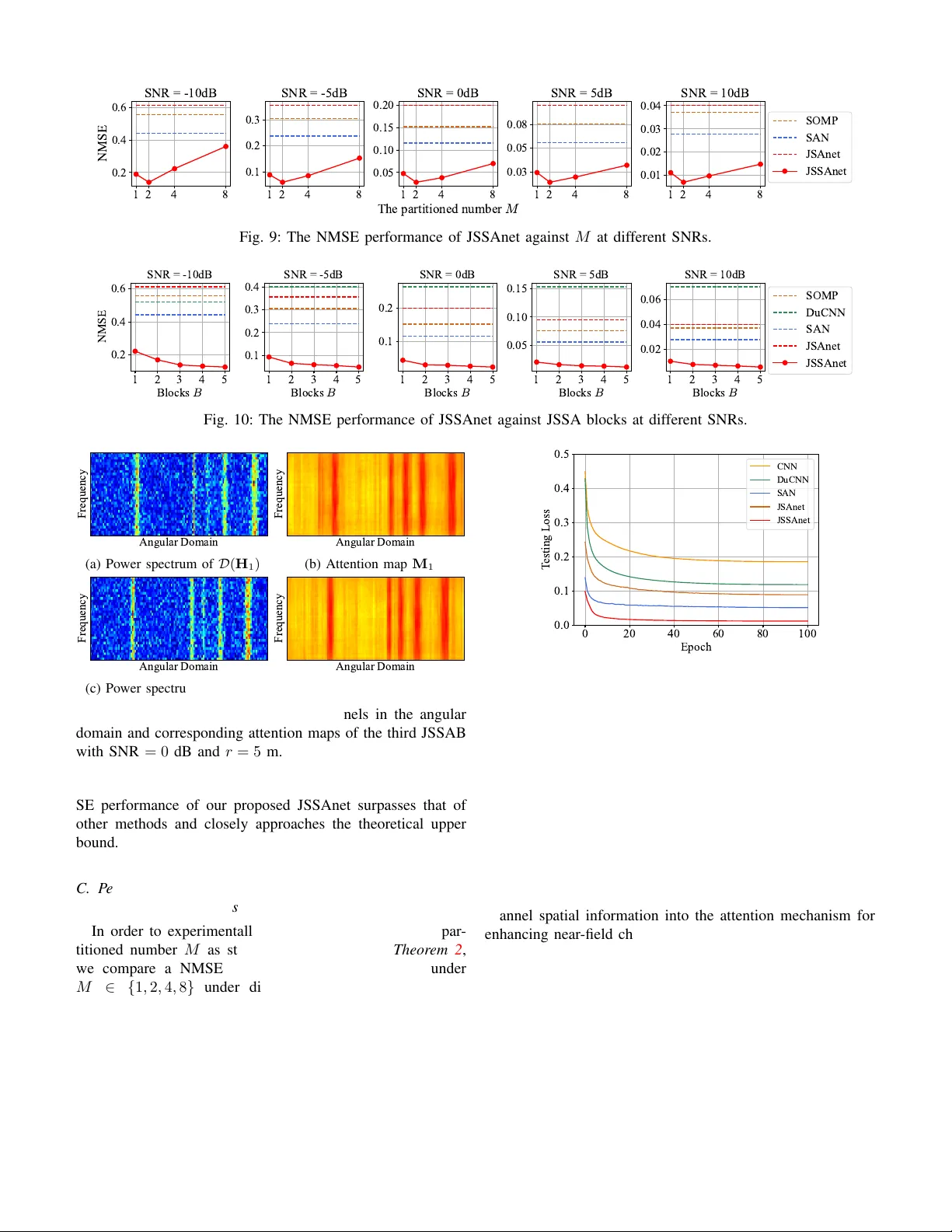
JSSAnet: Theory-Guided Subchannel Partitioning and Joint Spatial Attention for Near-Field Channel Estimation

1 JSSAnet: Theory-Guided Subchannel P artitioning and Joint Spatial Attention for Near -Field Channel Estimation Zhiming Zhu, Shu Xu, Student Member , IEEE , Chunguo Li, Senior Member , IEEE , Y ongming Huang, F ellow , IEEE , and Luxi Y ang, Senior Member , IEEE Abstract —The deployment of extremely lar ge-scale antenna array (ELAA) in sixth-generation (6G) communication systems introduces unique challenges for efficient near-field channel estimation. T o tackle these issues, this paper presents a theory- guided appr oach that incorporates angular inf ormation into an attention-based estimation framework. A piecewise F ourier repr esentation is proposed to implicitly encode the near-field channels inherent nonlinearity , enabling the entire channel to be segmented into multiple subchannels, each mapped to the angular domain via the discrete Fourier transform (DFT). Then, we develop a joint subchannel-spatial-atte ntion network (JSSAnet) to extract the spatial features of both intra- and inter -subchannels. T o guide theoretically the design of the joint attention mechanism, we derive upper and lower bounds based on approximation criteria and DFT quantization loss mitiga- tion, respectively . Following by both bounds, a JSSA layer of an attention block is constructed to assign independent and adaptive spatial attention weights to each subchannel in parallel. Subsequently , a feed-forward network (FFN) of an attention block further captures and refines the residual nonlinear de- pendencies across subchannels. Moreo ver , the proposed JSSA map is linearly computed via element-wise pr oduct combining large-ker nel convolutions (DLKC), maintaining strong contextual learning capability . Numerical results verify the effectiveness of embedding sparsity information into the attention network and demonstrate JSSAnet achiev es superior estimation performance compared with existing methods. Index T erms —ELAA, extremely large-scale MIMO, near- field channel estimation, subchannel partitioning, joint attention mechanism, deep lear ning. I . I N T R O D U C T I O N T HE sixth-generation (6G) communication systems are e x- pected to meet gro wing demands, such as the higher spec- tral efficienc y (SE) and enhanced spatial degrees of freedom (DoF) [ 1 ], [ 2 ]. Meanwhile, extremely large-scale multiple- input-multiple-output (XL-MIMO) is regarded as a promising paradigm to advance conv entional MIMO technologies, where extremely large-scale array (ELAA) is deployed to meet the expected demands of 6G [ 3 ], [ 4 ]. Z. Zhu, S. Xu, Y . Huang and L. Y ang are with the National Mo- bile Communications Research Laboratory , School of Information Sci- ence and Engineering, Southeast University , Nanjing 210096, China, and also with Purple Mountain Laboratories, Nanjing 211111, China (e- mail: { zhuzm, shuxu, huangym, lxyang } @seu.edu.cn). C. Li is with the National Mobile Communications Research Laboratory , School of Information Science and Engineering, Southeast Uni versity , Nanjing 210096, China (e-mail: chunguoli@seu.edu.cn). Compared with con ventional massi ve MIMO, the deplo y- ment of ELAA in v olves not only a significantly larger array aperture but also arises from a fundamental changes in electro- magnetic (EM) characteristics in the communication systems [ 5 ], [ 6 ]. The EM propagation field is di vided into near -field and far -field regions by the Rayleigh distance d R = 2 D 2 λ [ 7 ], that is determined by the array aperture D and signal wav elength λ . The extended Rayleigh distance of XL-MIMO increases the likelihood that the communication link builds in the near- field region. Unlike the planar wav efronts in far-field commu- nication, near -field propagation is characterized by spherical wa vefronts impinging on the antenna array . Consequently , the large number of antenna elements, combined with the paradigm shift in channel models, brings new challenges for near-field channel estimation [ 3 ], [ 4 ]. The expanded antenna aperture increases the size of the channel matrix, leading to the higher computational complexity in channel estimation. Spherical wav efronts introduce additional channel coefficients that need to be estimated. In recent years, near-field channel estimation has received significant attention. Classically , least squares (LS) and minimum mean squared error (MMSE) estimators are directly applied to near-field channel estimation without requiring channel model [ 8 ]. How- ev er , LS comes from a linear formulation of channel recon- struction and is sensiti ve highly to noise. Meanwhile, MMSE adopts channel statistical characteristics to generate a weight matrix to minimize the estimated errors of LS solutions. Howe v er , it is dif ficult to prepare the knowledge of channel correlation matrix, especially the ELAA brings the higher computation of matrix multiplication. Inspired by far-field channel estimation techniques, some approaches exploit the low-rank property of near -field channel matrices and employ the compressiv e sensing (CS) algo- rithms to estimate channel parameters. In con v entional channel estimation frameworks, the original channel matrix can be presented as a sparse angular representation by discrete Fourier transform (DFT) [ 9 ]. Howe ver , due to significant angular spread and beam squint in near-field channels, DFT -based representations become ineffecti ve for accurate channel esti- mation [ 10 ]–[ 12 ]. T o e xplore the near-field channel sparsity , studies in [ 13 ], [ 14 ] propose that the near -field channel is pro- jected into the sparse spatial location domain by the transform dictionaries. Subsequently , the orthogonal matching pursuit (OMP) algorithms are applied to estimate sparse channel coefficients and reconstruct the near-field channel. In [ 13 ], 2 the near-field transform matrix is constructed in the Cartesian domain by uniformly discretizing the communication coverage area into grids within the x - y plane. Alternatively , the authors of [ 14 ] propose the near-field channel is projected into the polar domain by discretizing both the distance and angle grids. Moreov er , the authors of [ 15 ] introduce a nov el discrete prolate spheroidal sequence (DPSS)-based eigen-dictionary for improving near-field channel estimation. As a critical implementation in the XL-MIMO, reconfigurable intelligent surface (RIS)-assisted channels are modeled under near -field conditions. In [ 16 ], the authors proposed extending the near- field RIS-aided channel dictionary is extended from two- dimensional (2D) to three-dimensional (3D) space in the x - y - z Cartesian coordinate system. W ith polar -based dictionaries, the sparse Bayesian learning (SBL) is employed to reconstruct parameters of the RIS channel in [ 17 ]. Howe ver , these ap- proaches incur the high computational overhead caused by the large-dimensional dictionary . T o address this issue, an efficient damped Ne wtonized OMP algorithm with hierarchical dictionaries in [ 18 ] is proposed to refine the path coef ficients layer in a layer-wise manner . Meanwhile, the works in [ 12 ] demonstrates that near-field channels exhibit angular sparsity and proposes an adaptive joint SBL algorithm that alternately refines angular and distance information for near-field or- thogonal frequency division multiplexing (OFDM) channel re- construction. Reference [ 19 ] designs a downsampled T oeplitz cov ariance matrix to decouple the angle and distance, followed by one-dimensional (1D) spatial search to joint estimate spatial angle-distance information of RIS-assisted channels. CS-based channel estimation algorithms share a common limitation, namely that estimation performance depends on the dictionary choice and stopping criterion. As an alternativ e choice, the machine learning (ML)-based channel estimation techniques has consequently been developed [ 20 ], [ 21 ]. In channel estimation tasks, the con volutional neural network (CNN) is employed to explore the spatial and frequenc y correlation of channels in [ 22 ]. The authors of [ 23 ] frame the channel estimation problem as an image denoising task, utilizing residual CNN to refine the coarse LS-based estimates. Motiv ated by channel sparsity , CNNs incorporating channel sparsity are proposed to enhance the denoising performance and robustness in [ 24 ], [ 25 ], where the coarse LS-based estimates and their sparse angular representations are simulta- neously fed into a dual CNN (DuCNN) architecture. Ho wev er , deep learning (DL)-based near-field channel estimation is still in its early stages. The works of [ 26 ] is exploiting CNN to extract spatial correlation of near-field channels for obtaining channel coef ficients. The model-assisted DL frame work, called the learned iterati ve shrinkage and thresholding (LIST A), is proposed for near-field channel estimation in [ 27 ], where the near-field transform dictionary is embedded into the deep neural network (DNN) in the IST A procedure. T o capture the nonlinear relationship of channel parameters, [ 28 ] proposes the DL-assisted scheme where the reco very problem is formulated in a probabilistic form. T o circumvent the exhausti ve search in [ 13 ], [ 29 ] treats near-field channel sparse representations as images and dev elops a keypoint detection network to estimate channel spatial information. In [ 30 ], the polar-based dictionary is employed in the IST A procedure to improve the near-field channel sparse reconstruction. Meanwhile, the transformer excels at the in-context learning (ICL) capabilities due to self- attention mechanisms [ 31 ], [ 32 ]. Although the self-attention mechanism demonstrate superior performance in conv entional channel estimation compared to other DL schemes [ 33 ], [ 34 ], the quadratic computational complexity of self-attention maps is impractical for the expanded near-field channel matrix. The study of [ 35 ] identifies CNN’ s poor adaptation to near-field non-stationarity , and the proposed spatial attention network (SAN) with linear complexity substantially outperforms CNN- based approaches. Howe ver , this approach fails to exploit the intrinsic sparse properties of near-field channels. In this work, we focus on dev eloping a joint attention-based near-field channel estimation framework that explicitly incor- porates spatial sparsity . Specifically , the main contributions of this work are as follows: • W e formulate near -field channel estimation as a denoising task on the LS-based coarse estimated channel. Inspired by [ 24 ], [ 25 ], [ 35 ], we propose a hybrid strategy that embeds sparse angular information into an attention- based neural network to enhance near-field channel esti- mation. T o av oid using expanded near-field dictionaries, the piecewise Fourier representation is introduced to implicitly and approximately encode the nonlinearity in the near-field channels utilizing the div erse spatial angles of subarrays. • Building on the piecewise Fourier representation, the channel is partitioned into subchannels, each of which is projected into angular domain via DFT . For theoretically guiding the design of the joint attention mechanism, we deriv e a theoretical lower bound on the piece wise number to satisfy the approximation criterion between the piecewise Fourier vector and near-field array response vector . In addition, we establish a theoretical upper bound to ensure that the angular div ersity among subchannels is maintained, thereby preserving critical spatial information after DFT . • W e propose a joint subchannel-spatial-attention network (JSSAnet) for near-field channel estimation. Cater to the channel partitioning, the design of attention blocks follows a decoupling-fusion strategy . First, a JSSA layer provides the personalized and independent spatial atten- tions for each subchannel in parallel. Second, a forward- feed network (FFN) layer is constructed to fuse extracted features across subchannels and model the nonlinear representations of near-field channel. Notably , our JSSA map is generated by the element-wise product combining decomposed large kernel con volutions (DLKC) for a linear computational complexity without compromising ICL capability . • Numerical results demonstrate both the ef fectiv eness of ELAA partitioning and the superior performance of our JSSAnet compared to other near-field channel estimation schemes. Ablation studies verify that jointly focusing on subchannel spatial sparsity significantly enhances the accuracy of near-field channel estimation. 3 BS r ( 0) 1 r ( 0) r ( 1 ) N r u se r u se r r e f e r e nc e e le me nt u se r u se r Fig. 1: The near-field uplink channel with spherical-wav e and with se veral scatters. The remainder of this paper is or ganized as follo ws. Sec- tion II introduces the near-field OFDM channel model and formulates the channel denoising task. Next, III present the representation of piecewise Fourier vector for the steering vector . Subsequently , in Section IV , the proposed JSSAnet is introduced in detail. Simulation results are provided in Section V . Finally , Section VI concludes this paper . Notation: W e use the following notations throughout the paper . A is a matrix; a is a vector; a is a scalar; the super- scripts ( · ) ∗ , ( · ) T , ( · ) H and ( · ) − 1 stand for conjugate operator , transpose operator , conjugate transpose operator and matrix in verse, respecti vely; ∥ A ∥ F and tr( A ) are the Frobenius norm and trace of A , respectiv ely; I N is the N × N identity matrix; [ a ] i and [ A ] i,j denote i -th entry of a and entry at the i -th row and j -th column of A ; x ∼ C N ( a , A ) is a complex Gaussian vector with mean a and cov ariance matrix A . E {·} is used to denote expectation; ⌈·⌉ and ⌊·⌋ are ceiling and floor operations, respectiv ely; ⊗ and ⊙ denote the Kronecker product and element-wise product, respecti vely; C ( X ) = R X 0 cos( π x 2 2 )d x and S ( X ) = R X 0 sin( π x 2 2 )d x are Fresnel functions. I I . S Y S T E M M O D E L A N D P RO B L E M F O R M U L AT I O N A. System Model W e consider an uplink time division duplexing (TDD) narrowband OFDM system with K subcarriers, as shown in Fig. 1 . The base station (BS) with N BS -antenna uniform linear array (ULA) and N RF RF chains is assumed to communicate with U single-antenna users, where the antenna spacing d = λ 2 is the half of signal wavelength. The pilot sequences emitted by users to the BS and the channel fading remain constants during the uplink channel estimation period. In this paper , we adopt the orthogonal pilot strate gy such that the channel estimation for each user is independent and a specific user is selected [ 14 ], [ 36 ]. W ithout loss of generality , one can choose the pilot signal s t,k = 1 in the t -th time slot on subcarrier k . W e collect the receiv ed pilots during T instants into a vector y k ∈ C T N RF × 1 on subcarrier k and stacking these from all subcarriers into a matrix, we have obtain the overall measurement matrix Y = [ y 1 , · · · , y K ] ∈ C T N RF × K as [ 12 ], [ 14 ] Y = W H H + V , (1) where W = [ W 1 , · · · , W T ] ∈ C N × T N RF is a combining matrix composed by the receive combining matrix W t of size N BS × N RF for t ∈ { 1 , · · · , T } and V = [ v 1 , · · · , v K ] of size T N RF × K is defined as the effecti ve noise matrix, where v k = W H n k of size T N RF × 1 and n k ∼ C N (0 , σ 2 I N BS ) is the noise vector with the noise po wer σ 2 . Note that the entries of W are chosen randomly from 1 √ N BS {− 1 , +1 } . Besides, H = [ h 1 , · · · , h K ] ∈ C N BS × K denotes a multi-subcarrier channel matrix whose k -th column vector h k ∈ C N BS × 1 is the channel of a certain user on subcarrier k . B. Channel Model W e commence with the near-field mmW av e channel in the spatial domain. As depicted in Fig. 1 , we consider the users locate at the near-field region of BS. Therefore, EM wa ve are incident on the antenna array of BS with the form of spherical wavefront. Then, we adopt the widely used extended Saleh-V alenzuela multipath channel model in the frequency domain. Then, the near-field channel h k for subcarrier k can be presented as h k = r N BS L L X ℓ =1 α ℓ e 2 π τ ℓ f k a ( θ ℓ , r ℓ ) , (2) where L ≪ N is the number of resolv able paths, α ℓ and τ ℓ are the complex gain and the time delay of the ℓ -th path, respectiv ely . The variable r ℓ is the distance from a scatter to a reference element of antenna array in BS for the ℓ -th path. The variable θ ℓ is the sine of the physical AoA ϕ ℓ corresponding to r ℓ , i.e., θ ℓ = sin ϕ ℓ . Then, ϕ ( n ) ℓ is the physical AoA of the n -th element where n = 0 , 1 , · · · , N BS − 1 . In this paper, the ( N BS 2 − 1) -th element is set as the reference element of the ELAA, i.e., θ ℓ = θ ( N BS / 2 − 1) ℓ and r ℓ = r ( N BS / 2 − 1) ℓ . Finally , a ( θ ℓ , r ℓ ) is the normalized antenna array response vector (AR V) at the BS. For the N BS -element ULA, a ( θ ℓ , r ℓ ) is written as a ( θ ℓ , r ℓ ) = 1 √ N BS  e j 2 π λ  r (0) ℓ − r ℓ  , · · · , e j 2 π λ  r ( N BS − 1) ℓ − r ℓ   H , (3) where r ( n ) ℓ for n ∈ { 0 , 1 , · · · , N BS − 1 } denotes the distance from a scatter to n -th antenna element for the ℓ -th path component. In the far-field communication, planar wav efronts lead to the linear distance dif ference of arriv al of EM wav es, which is calculated by r ( n ) ℓ − r ℓ = − ∆ n dθ ℓ , (4) where ∆ n = n − N BS 2 + 1 is the index interv al between the n -th element and the reference element, i.e., ∆ n = − N BS 2 + 1 , − N BS 2 + 2 , · · · , N BS 2 . Howe v er , spherical wavefronts in the near-field commu- nication result in the distance differences of arrival of EM wa ves is non-linear with respect to the antenna index n . Accordingly , the distance difference of arri val for the ℓ -th path is approximately expressed as [ 12 ] r ( n ) ℓ − r ℓ ≈ 1 − θ 2 ℓ 2 r ℓ d 2 ∆ 2 n − ∆ n dθ ℓ . (5) It rev eals that the explicit distinction of expressions be- tween near-field and far -field channels lies in the presence of quadratic term in the phase term. 4 C. Near-field Channel Estimation F ormulation As we know , ( 1 ) is a typical linear expression of pilot- based mmW av e channel estimation, and various methods are rendered, including the LS algorithm, the linear minimum mean squared error (LMMSE) algorithm, the CS approach and the DL approach. 1) LS algorithm: The LS algorithm originated from min- imizing    y k − W H ˆ h k    2 . Hence, the estimated channel ˆ h LS k for subcarriers k by LS estimator is expressed as ˆ h LS k =  WW H  − 1 Wy k . (6) Hence, the LS-based estimated channel for all subcarriers ˆ H LS is ˆ H LS = [ ˆ h LS 1 , ˆ h LS 2 · · · , ˆ h LS K ] . 2) LMMSE algorithm: The LS algorithm has lo w comple xity but poor performance in low-SNR regime. Therefore, employ- ing the weighted matrix is to minimize the euclidean distance between the true channel and the LS-based estimated channel. The estimated channel ˆ h LMMSE k for subcarrier k by LMMSE estimator can be obtained by ˆ h LMMSE k = R h k ˆ h LS k  R h k h k + σ 2 I N BS  − 1 ˆ h LS k , (7) where R h k ˆ h LS k is the cross correlation matrix between h k and ˆ h LS k , and R h k h k is the autocorrelation matrix of h k . Hence, the LMMSE-based estimated channel for all subcarriers ˆ H LMMSE is ˆ H LMMSE = [ ˆ h LMMSE 1 , ˆ h LMMSE 2 , · · · , ˆ h LMMSE K ] . 3) CS appr oach: The LS and LMMSE algorithms ignore the inherent property of the mmW ave channels. Thus, the CS approach is employed to reconstruct the mmW ave channel by exploiting the sparse spatial nature from poor scatters, where channel representations are found from redundant dictionaries. This problem can be presented as minimizing a ℓ 0 -norm function [ 37 ] and given by min ∥ x k ∥ 0 , s . t . y k = W H Φx k , (8) where Φ ∈ C N BS × D and x k ∈ C D × 1 are the transform dictionary of size D for h k and a sparse vector , respectively . Note that the CS-based schemes are highly sensitive to dic- tionary selection and the stopping criteria setting. In far-field communication scenarios, the DFT matrix is chosen as the dictionary Φ because its array response vector is discrete Fourier vector . Howe ver , the in volv ed distance information makes DFT matrix inef ficient in near-field channel estimation. Consequently , the design of near-field dictionaries has become an acti ve area of research [ 12 ], [ 14 ]. 4) DL appr oach: DL-based approaches are widely applied in channel estimation. The channel estimation procedure is typi- cally transferred to a signal denoising task in the existing DL- based schemes [ 23 ]–[ 25 ]. In the procedure, the pre-estimated channel from LS estimator is fed into the developed neural network which the output of is vie wed as improved channel reconstruction. The DL-based channel estimation procedure can be con- cluded into two phases: offline training phase and online estimation phase . Let the training set S t with size of ∥S t ∥ and testing set ˙ S t with size of ∥ ˙ S t ∥ denote as S t = n H (1) LS , H (1)  , · · · ,  H ( ∥S t ∥ ) LS , H ( ∥S t ∥ ) o (9) and ˙ S t = n ˙ H (1) LS , ˙ H (1)  , · · · ,  ˙ H ( ∥ ˙ S t ∥ ) LS , ˙ H ( ∥ ˙ S t ∥ ) o , (10) respectiv ely , where H ( i ) LS and ˙ H ( i ) LS are the i -th noisy channel from LS observ ations, and H ( i ) and ˙ H ( i ) are corresponding true channels. Note that there is no overlap between S t and ˙ S t . The forward propagation process and parameters of the neural network are defined as F Θ ( · ) and Θ , respectively . In training phase, the training set S t is sent into the designed neural network and back propagation refines the parameters Θ of F Θ ( · ) aiming to minimize the loss function. In general, the empirical mean square error (MSE) criterion is utilized to the loss function, i.e., L ( Θ ) = 1 ∥S t ∥ ∥S t ∥ X i =1    H ( i ) − F Θ  H ( i ) LS     2 F . (11) Consequently , it is achieved the well-trained network with the trained parameters Θ ∗ . In online estimation phase, the well-trained netw ork F Θ ∗ processes the testing data ˙ H LS sampled from ˙ S t . The estimated channel ˆ H net is obtained by ˆ H net = F Θ ∗  ˙ H LS  . (12) In this work, we also adopt this framew ork to formulate the channel estimation problem as an LS estimation denoising task and the detail of our neural network will be provided in following sections. I I I . P I E C E W I S E L I N E A R A P P R O X I M A T I O N As a data-driven approach, the performance of DNN-based channel estimation strongly depends on its ability to extract discriminativ e features from input data. Sev eral strategies are explored to improve the representation capacity of neural net- works for mmW ave channels. First, a self-attention mechanism is integrated into effecti vely model inter-element dependencies within the channel matrix to suppress noise. Second, inspired by CS approach exploring the inherent sparsity , the mmW av e channel is projected into the angular domain via DFT and the neural network extracts its sparse features to enhance denoising performance, as demonstrated in [ 24 ], [ 25 ]. Inspired by these strategies, we propose a hybrid strategy for the near-field channel estimation, in which the sparse angular representations are embedded into the attention procedure. Howe v er , existing transform dictionary ine vitably expand the size of sparse representation matrix for XL-MIMO commu- nications, which substantially raises the computational cost of neural networks. Meanwhile, ( 5 ) indicates that the time differences of arriv al exhibit a nonlinear property with respect to the antenna inde x. The non-ne gligible angular energy spread significantly degrades the ef ficiency of DFT in sparsely rep- resenting near-field channels [ 12 ]. This section presents an approximate representation of the near-field AR V using a piece wise linear vector compatible with the DFT . Then, a theoretical lower bound on the piece wise number is deri ved to satisfy the approximation criterion. Furthermore, a theoretical upper bound is established to ensure 5 suba r ra y 1 suba r ra y 1 r 2 r suba r ra y 2 …… …… 1 2 M r M M Fig. 2: The ELAA is partitioned uniformly into M subarrays. The EM wa ves impinge on the subarray with planar wa vefront, while the wa vefronts between subarrays exhibit spherical wa ves. that angular div ersity across subchannels is maintained in the angular-domain projection. A. The Piecewise Linear Approximation of the Near-field ARV Giv en the non-linearity of near -field XL-MIMO channels, it is an alternative approach that the near-field AR V is approxi- mately decomposed into multiple linear vectors catering to the linearity of DFT . In this work, the ELAA of BS is partitioned uniformly into M subarrays of size N , where M = ⌈ N BS N ⌉ . Then, the antenna index set is S i = { ( i − 1) N , · · · , iN − 1 } for i ∈ { 1 , 2 , · · · , M } . Accordingly , we choose the n i -th element as the reference element corresponding to the i -th subarray , where n i = iN − N 2 − 1 . Here, we focus on a certain path component. For the sake of notation, omit the subscript ℓ and define θ 0 and r 0 as reference AoA and distance for the entire array . Recall ( 3 ) and ( 5 ), the phase difference of arriv al is defined as p n corresponding to n -th antenna element, given by p n = − 2 λ  r ( n ) − r 0  ≈ − 1 − θ 2 0 2 r 0 d ∆ 2 n + ∆ n θ 0 , (13) and the deriv ation with respect to the index interval ∆ n is p ′ n = − 1 − θ 2 0 r 0 d ∆ n + θ 0 . (14) Then, expanding with first-order T aylor series at the refer - ence element of the i -th subarray n = n i , we have p n = p n i + p ′ n i ( n − n i ) + O ( n ) . (15) Suppose the scatter locates at ( x, y ) and the coordinate of n -th element is (0 , ∆ n d ) , the spatial AoA θ ( n ) and distance r ( n ) between the scatter and n -th element are computed by    θ ( n ) = y − ∆ n d r ( n ) , r ( n ) = p x 2 + ( y − ∆ n d ) 2 . (16) Then, expanding with first-order T aylor series at the reference element,i.e., n = N BS 2 − 1 , we hav e θ ( n ) = θ 0 − 1 − θ 2 0 r 0 d ∆ n + O ( n ) ≈ p ′ n . (17) 1 2 4 8 16 32 Number of subarray M 0 0.1 0.2 0.3 0.4 0.5 0.6 0.7 0.8 0.9 1 Similarity metric j S j N B S = 256 N B S = 512 N B S = 1024 3 dB Fig. 3: The similarity metric between b ( θ ) and a ( θ 0 , r 0 ) . The carrier frequency f c , the spatial AoA θ 0 and distance r 0 are 60 GHz, sin( π / 12) and 15 meters, respectiv ely . Substituting ( 17 ) into ( 15 ), the approximate phase vector p i of the near-field AR V corresponding to i -th subarray can be linearly written as p i ≈ h p n i + mθ ( n i ) i N 2 m = − N 2 +1 , (18) where m ≜ n − n i ∈  − N 2 + 1 , − N 2 + 2 , · · · , N 2  . It indicates that the exponential term of the subarray response vector can approximately be composed by two parts: time difference of arri val p n i and spatial AoA θ ( n i ) corresponding to the reference element of the subarray . For clarity , we define ˜ p i ≜ p n i , ˜ r i ≜ r ( n i ) and ˜ θ i ≜ θ ( n i ) . Subsequently , according to ( 18 ), the array response vector of the i -th subarray is approximately rewritten as [ a ( θ 0 , r 0 )] S i ≈ r N N BS e j π ˜ p i b ( ˜ θ i ) , (19) where b ( ˜ θ i ) = 1 √ N h 1 , e j π ˜ θ i , · · · , e j π ( N − 1) ˜ θ i i T ∈ C N × 1 is a Fourier vector . It is observed that the subarray response vector is consisted of a free-space phase delay f actor of subarray i and a linear Fourier vector with size of N × 1 . Thus, collecting linear subarray response vectors, the array response vector a ( θ 0 , r 0 ) can be piecewise represented by b ( θ ) = r N N BS h e j π ˜ p 1 b ( ˜ θ 1 ) T , · · · , e j π ˜ p M b ( ˜ θ M ) T i T , (20) where θ = [ ˜ θ 1 , ˜ θ 2 , · · · , ˜ θ M ] . Therefore, the near-field AR V can be approximated as a piecewise Fourier vector . It is consistent with intuition that the case of a user locating at the near-field region of the ELAA can be equi valent to that of a user locating at the far -field regions of partitioned subarrays. As sho wn in Fig. 2 , the entire antenna array is divided uniformly into M subarrays. It is assumed that EM wa ves impinging on each subarray can be modeled as planar , while the wavefronts between subarrays exhibit spherical characteristics.Essentially , the piecewise Fourier vector implicitly encodes the nonlinear spatial information of near-field AR V utilizing the different AoAs across subarrays. 6 B. Discussion on Number of Subarrays Intuitiv ely , the number of partitions determines the fidelity of the piece wise Fourier vector in approximating the near-field AR V a ( θ 0 , r 0 ) . From a theoretical perspective, an insufficient number makes it difficult for the piecewise Fourier vector to precisely approximate the near-field AR V . Theor em 1: If the piecewise Fourier vector can approxi- mately present the near-field AR V , the partitioned number M must satisfy M ≥ & r d r min N BS 4 ' , (21) where r min is the minimum feasible distance in communication system. Pr oof: See Appendix A . ■ According to Theor em 1 , for a 512 -ULA, the partitioned number must satisfy the condition of M ≥ ⌈ 2 . 86 ⌉ = 3 . For implementation con venience, M is set to be a power of 2 , i.e., M = 4 . As shown in Fig. 3 , we present the similarities between b ( θ ) and a ( θ 0 , r 0 ) corresponding to various array sizes. It can be observed that for ULAs with N BS ∈ { 256 , 512 , 1024 } , the corresponding minimum v alues of M are 2, 4 and 8, respectively , which v alidate the abov e theorem of M ≥ ⌈ 1 . 43 ⌉ , M ≥ ⌈ 2 . 86 ⌉ and M ≥ ⌈ 5 . 72 ⌉ . While partitioning the ELAA facilitates the transformation of the channel into the angular domain, it ine vitably reduces the spatial angular resolution of each recei ve subarray , as resolution is proportional to the array aperture. Therefore, the degradation in angular resolution imposes a practical upper limit on the partitioned number that can be employed. T o elaborate, as shown in Fig. 2 , the near-field channel can be stacked by M subchannels, i.e., H =  H T 1 , H T 2 , · · · , H T M  T , (22) where H i = [ h ( i ) 1 , · · · , h ( i ) K ] ∈ C N × K is the i -th subchannel between the user and subarray i for all subcarriers and h ( i ) k is the i -th subchannel at subcarrier k . Accordingly , the angular- domain piecewise representation of H is determined by the subchannels H i , i.e., D ( H ) = ( I M ⊗ Φ ) H H =  ( Φ H H 1 ) T , ( Φ H H 2 ) T , · · · , ( Φ H H M ) T  T , (23) where Φ = [ b ( φ 1 ) , b ( φ 2 ) , · · · , b ( φ N )] is a unitary DFT matrix with size of N × N and φ n = 1 N ( n − N +1 2 ) for n = 1 , 2 · · · , N . Accordingly , the beam pattern vector c ( i ) k,ℓ of the ℓ -th path component corresponding to h ( i ) k in angular domain is determined as c ( i ) k,ℓ = Φ H b ( ˜ θ ℓ,i ) = [Ξ( ˜ θ ℓ,i − φ 1 ) , Ξ( ˜ θ ℓ,i − φ 2 ) , · · · , Ξ( ˜ θ ℓ,i − φ N )] T , (24) where ˜ θ ℓ,i is the spatial AoA of the ℓ -th path for subarray i and Ξ( x ) = sin N π x N sin πx is the Dirichlet sinc function, whose power is concentrated near x = 0 . Thus, | [ c ( i ) k,ℓ ] n | 2 presents the po wer of the n -th entry of c ( i ) k,ℓ . It has been observed that the adverse ef fects of near- field conditions on channel estimation become increasingly 10 15 20 25 Degree ( / ) 0 0.2 0.4 0.6 0.8 1 Normalized j [ c ( i ) k;` ] n j 2 b ( ~ 3 `; 1 ) b ( ~ 3 `; 2 ) n = 80 n = 81 (a) M = 2 10 15 20 25 Degree ( / ) 0 0.2 0.4 0.6 0.8 1 Normalized j [ c ( i ) k;` ] n j 2 b ( ~ 3 `; 1 ) b ( ~ 3 `; 2 ) b ( ~ 3 `; 3 ) b ( ~ 3 `; 4 ) n = 40 n = 41 (b) M = 4 Fig. 4: The normalized power distributions of c k,ℓ for the ℓ -th path component at f k = 60 GHz, where N BS = 256 , ϕ ℓ = 15 ◦ and r ℓ = 20 meters. (a) The case of M = 2 ; (b) The case of M = 4 . pronounced as users move closer to the BS [ 12 ], [ 38 ]. T o guarantee the lower bound of near-field channel estimation, it is required that beam patterns of subchannels represented by different Fourier vectors of Φ within the region of the mini- mum feasible propagation distance, i.e., arg max n | [ c ( i ) k,ℓ ] n | 2  = arg max n | [ c ( j ) k,ℓ ] n | 2 for i  = j when r = r min . Ho wev er , as the subarray aperture decreases below a certain threshold, it inevitably leads to cases where at least two subchannels exhibit a nearly identical angular distribution. For e xample, a near- field scenario with N BS = 256 , ϕ ℓ = 15 ◦ and f c = 60 GHz is considered, the po wer distrib utions of beam patterns of the ℓ -th path component are shown in Fig. 4 . W e observe that when the ELAA is partitioned into 2 subarrays, each subchannel e xhibits a dominant beam pattern with a distinct index, namely , [ c (1) k,ℓ ] 80 and [ c (2) k,ℓ ] 81 . Howe ver , when the ELAA is partitioned into 4 subarrays, subchannel 1 and 2 share the same dominant beam, namely , b ( φ 40 ) and [ c (1) k,ℓ ] 40 ≈ [ c (2) k,ℓ ] 40 . Therefore, D ( H 1 ) and D ( H 2 ) share almost common spatial angular features, making it dif ficult for the neural network to extract the specific spatial features of different subchannels. Accordingly , we provide the upper bound on the number of subchannels below . Theor em 2: If the number of partitioned subarrays M only satisfies M ≤     s (1 − θ 2 sec ) d 2 r min N BS     , (25) an DFT matrix with size of N × N preserves diverse angular information across subchannels when channel near-field effect with r = r min is most pronounced. Pr oof: See Appendix B . ■ 7 JSS AB - B LN JS SA F F N LN JSS AB - B LN JS SA F F N LN Co n v 1 JSS AB - 1 Co n v 2 Co n v 2 JSS A B × B in X 0 F 1 F e s t X Re fin e T a il El e me n t - w i se A d d i t i o n El e me n t - w i se A d d i t i o n F ea t u r e E emb d i n g F ea t u r e E emb d i n g F ea t u r e R ed u ce F ea t u r e R ed u ce () () 1 () 1 () 2 F (a) The structure of the proposed JSSAnet for near-field channel estimation. DW DW DWD DWD PW PW PW PW PW PW DW DW DW DWD PW PW PW DW DW DW DW D DW D PW PW PW PW PW PW DW DW DW DW D PW PW PW DW DW DWD PW PW PW DW DW DW D PW PW PW DW DW DW DW D DW D PW PW PW PW PW PW DW DW PW PW PW PW PW PW DW DW DW DW DWD DWD DW DW D PW PW PW DW PW PW PW DW DW DWD PW PW M b X b A i V i Q i K i P DW DWD PW PW PW DW DW DW D PW PW PW DW DW DW D PW PW PW DW PW PW PW DW DW DWD PW M b X b A i V i Q i K i P (b) Joint Subchannel-Spatial-Attention (JSSA) Module DW DW PW PW PW PW A X F X DW PW PW A X F X (c) Forward-feed network (FFN) PW PW PW PW DW DW D WD D WD PW PW T X R X PW PW DW D WD PW T X R X (d) Refine T ail Fig. 5: Decomposition of the proposed JSSAnet: Overall Architecture and functional Modules. In this work, we propose to decompose the near-field chan- nel into multiple subchannels and embed their joint angular representations into the attention-based channel estimation framew ork. Meanwhile, Theorem 1 and Theor em 2 provides the theoretical bounds for the number of partitioned subchan- nels for the design of our neural network. I V . J O I N T S U B C H A N N E L - S PA T I A L - A T T E N T I O N N E T W O R K F O R N E A R - F I E L D C H A N N E L E S T I M A T I O N In this section, we propose a joint subchannel-spatial- attention network (JSSAnet) for near-field channel estimation based on the ELAA partitioning strategy . The network pro- vides mutually independent and personalized attention to the distinct spatial information of each subchannel in parallel, while also fusing inter -subchannel information to model the nonlinear representation for near-field channels. A. The Structur e Design of JSSAnet As sho wn in Fig. 5a , the proposed JSSAnet applies a standard autoregressi ve architecture with a residual shortcut connection, integrating multiple functional modules to imple- ment near-field channel estimation. In detail, a DFT operation D ( · ) and an in verse DFT (IDFT) operation D − 1 ( · ) provide bi-directional mapping between the channel matrix and its angular -domain representation. The con volutional layers Conv 1 and Con v 2, both with { 3 , 1 } 1 are utilized to embed features 2 to C > 2 and reduce features back to the original input dimension before IDFT operation, respec- tiv ely . Notice that Con v 1 performs feature embedding on M 1 W e denote { a, b } as the conv olution layer, where a is a a × a filter , b is a stride of b . 2 W e adopt ‘feature’ as the replacement term to avoid confusion with ‘channel’ of the communication system in this paper . subchannels simultaneously and independently and features of subchannels are stacked to F 1 ∈ R N BS × K × C . B consecutive joint subchannel-spatial-attention blocks (JSSABs) are main body , enabling joint exploitation of subchannel spatial sparsity . T o further enhance feature representation, a refinement tail module is appended after the final JSSAB to fuse and refine features across all subchannels. B. DFT and IDFT Operations Different from traditional near-field channel estimation based on attention mechanisms, we exploit the prior infor- mation of channel sparsity in an attention procedure. Prior studies have extensi vely in vestigated the sparse representation of near-field channels [ 39 ], [ 40 ]. Howe ver , the expanded dictionaries, due to the additional spatial distance information, inevitably increase the size of the sparse matrix, raising the computational overhead. Accordingly , the channel is divided into M subchannels with size of N × K , and each subchannel is projected into the angular domain using an DFT matrix Φ with size of N × N , following a piece wise Fourier vector representation. Based on Theorem 1 and Theor em 2 , the channel is sepa- rated uniformly into M subchannels and each subchannel is con verted into an angular representation matrix by Φ before Con v 1. The output F 2 ∈ R N BS × K × 2 of Con v 2 is conv erted to the estimated channel matrix through IDFT operation. Since the neural network processes real-valued data, the real and imaginary parts of the complex channel matrix are decom- posed and stacked into a 2-feature tensor . Then, the input and corresponding true channel labels of datasets ( 9 ) and ( 10 ) are processed as X in . = {ℜ ( H LS ) , ℑ ( H LS ) } ∈ R N BS × K × 2 , (26) X gt . = {ℜ ( H ) , ℑ ( H ) } ∈ R N BS × K × 2 . (27) 8 Then, ( 23 ) is re written as the DFT operation on tensor X in 3 to obtain tensor F 0 4 , i.e., D ( X in ) =  ℜ ( ˜ Φ ) T ℑ ( ˜ Φ ) T −ℑ ( ˜ Φ ) T ℜ ( ˜ Φ ) T   X in,1 X in,2  =  F 0 , 1 F 0 , 2  , (28) where ˜ Φ = I M ⊗ Φ . The angular-domain tensor cor - responding to subchannel H i is [ F 0 ] i ∈ R N × K × 2 , i.e., [ F 0 ] i ≜ [ F 0 ] ( i − 1) N : iN , : , : for i = 1 , 2 , · · · , M . [ F 0 ] i for i = 1 , 2 , · · · , M are concatenated along the first dimension, we hav e F 0 . = { [ F 0 ] 1 ; [ F 0 ] 2 ; · · · ; [ F 0 ] M } . (29) The IDFT operation on F 2 ∈ R N BS × K × 2 is written by D − 1 ( F 2 ) =  ℜ ( ˜ Φ ) −ℑ ( ˜ Φ ) ℑ ( ˜ Φ ) ℜ ( ˜ Φ )   F 2 , 1 F 2 , 2  =  X est,1 X est,2  , (30) where X est . = {ℜ ( ˆ H ) , ℑ ( ˆ H ) } ∈ R N BS × K × 2 is the estimated channel tensor by the JSSAnet, i.e., ˆ H = X est,1 + j X est,2 . C. The Implementation of JSSAB Cater to the ELAA partitioning, the design of JSSAB follows a decoupling-fusion strate gy , that subchannels are first decoupled and processed independently in the joint subchannel-spaital-attention (JSSA) layer and the extracted features of subchannels are fused in a forw ard-feed netw ork (FFN) layer , as described in Fig. 5a . T o preserve instance- specific details, a layer normalization (LN) layer is applied prior to both the JSSA and FFN layers. 1) JSSA layer: As a ke y layer of JSSAB, the JSSA layer provide the personalized and independent attentions for individual subchannels in parallel. Specifically , the unique spatial features of each subchannel are emphasized indepen- dently and simultaneously through their dedicated attention implementations. As shown in Fig. 5b , the input tensor X b ∈ R N BS × K × C for b = 1 , · · · , B is divided to M segments { [ X b ] i ∈ R N × K × C } M i =1 along the first dimension by the channel-split operation, with each segmented tensor corresponding to one subchannel, i.e., [ X b ] i corresponds to the feature tensor of D ( H i ) . Subsequently , all segmented tensors [ X b ] i are processed in parallel through their respectiv e attention implementations. Here, we illustrate the attention implementation correspond- ing to the i -th subchannel in JSSAB. As shown in Fig. 5b , the query Q i ∈ R N × K × C , ke y K i ∈ R N × K × C , and v alue K i ∈ R N × K × C for i -th subchannel at the b -th JSSAB are constructed from [ X b ] i as Q i = f DW ( f P W ([ X b ] i )) , (31) K i = f DLK C ( f P W ([ X b ] i )) , (32) V i = f P W ([ X b ] i ) , (33) where f DW ( · ) , f P W ( · ) and f DLK C ( · ) denote the depth-wise (D W) con v olution, the point-wise (PW) con v olution and the decomposed large-kernel con volution (DLKC), respectively . 3 Denote X in,i as the i -th feature matrix of tensor X in . e.g., X in,1 = ℜ ( H LS ) and X in,2 = ℑ ( H LS ) . 4 Denote F j,i as the i -th feature matrix of tensor F j . Then, the ( Q i , K i , V i ) projection P i for subchannel i can be written as M i = Q i ⊙ K i , (34) P i = M i ⊙ V i , (35) where M i is spatial-attention map for the subchannel i . Accordingly , M joint attention implementations comprise our JSSA mechanism. Equations ( 34 ) and ( 35 ) indicate the proposed JSSA differs from the used widely self-attention. The JSSA mechanism adopt the element-wise product to calculate the individual attention map of the subchannel, rather than matrix multi- plication. Although the element-wise product implements a lightweight attention mechanism, it inherently suffers from limitations in modeling global contextual features compared to the matrix multiplication. T o address this issue, DLKC is introduced to enhance the attention mechanisms capability of capturing long-range dependencies, owing to its expanded large receptiv e field. In essential, the DLKC is a lo w complex- ity v ariant of the large-kernel conv olutions (LKC) proposed in [ 41 ]. In detail, a LKC with an a × a filter is decomposed into the cascading (2 d − 1) × (2 d − 1) depth-wise (D W) f DW ( · ) , ⌈ a d ⌉ × ⌈ a d ⌉ depth-wise dilation (D WD) f DW D ( · ) with dilation d and point-wise (PW) f P W ( · ) con volutions. The decomposition process is formulated as DLKC, i.e., f DLK C ( · ) = f P W ( f DW D ( f DW ( · ))) . Moreov er , it is clear that the projection of the proposed attention map removes the softmax function typically used in standard self-attention mechanisms, whose effecti veness in recognition tasks has been demonstrated in [ 41 ]. In total, the computational complexity of calculating JSSA maps grows linearly with the ELAA aperture, i.e., the order of O ( N BS ) . Subsequently , the projections for all subcannels are con- catenated to a tensor P b along the first dimension, i.e., P b = { P 1 ; P 2 ; · · · ; P M } and P b is sent into the PW con- volution to fuse cross-subchannel spatial features and obtain A b ∈ R N BS × K × C . 2) FFN layer: The FFN layer plays a crucial role in transformer networks. Gi ven that the global characteristics of the near-field channel are distributed among subchannels, the FFN in JSSAB aims to fuse the independent ly e xtracted spatial features from the JSSA layer, enhancing the nonlinear representation of JSSAnet. T o reduce computational overhead, we replace fully connected layers with a lightweight attention module comprising DW and PW con v olutions, as illustrated in Fig. 5c . Given the tensor X A ∈ R N BS × K × C from the LN layer , the flow procedure of FFN is represented as X F = f P W ( X A ) ⊙ f DW ( f P W ( X A )) . (36) D. Implementation of Refine T ail W e employ the refine tail module in the tail of the au- toregressi ve attention backbone. In detail, the large-k ernel attention (LKA) module proposed in [ 41 ] with a DLKC is enclosed between two PW con volutions as shown in Fig. 5d . The refine tail module emphasizes the refinement of spa- tial representations across dif ferent subchannels. On the one 9 T ABLE I: The Simulation Dataset Configurations Parameters V alue The number of BS antennas N BS 256 Carrier frequency f c 60 GHz Bandwidth f B 100 MHz The number of subcarriers K 32 The number of paths L L ∼ P oisson (6) The distribution of angle ϕ ϕ ∼ U ( − π 3 , π 3 ) The Rayleigh distance d R 163 . 84 m The distance between BS and user r r ∼ U (5 , d R ) m Channel model realization Extended Saleh-V alenzuela Signal-to-noise ratio SNR (dB) {− 10 , − 5 , 0 , 5 , 10 } Dataset size 2 × 10 4 Dataset split (train:test) 4 : 1 T ABLE II: Training Settings of the JSSAnet Parameters V alue Embedding features C 20 Con v1, Conv2 { 3 , 1 } DLKC (DW -DWD-PW) 35 : 7 - 9(4) - 1 DW of the FFN { 7 , 1 } The partitioned number M 2 JSSA blocks B 3 Batch size 32 T raining epoch S 100 Learning rate γ t γ 0 = 1 × 10 − 3 with warmup Scheduler Cosine annealing strategy T raining optimizer Adam optimizer W eight decay 1 × 10 − 4 hand, all subchannel features with size of N × K × C are concatenated into a composite image for processing by the LKA, which enhances inter-subchannel dependencies. On the other hand, it facilitates fine-grained information extraction tailored to individual subchannels. V . N U M E R I C A L R E S U LT S In this section, we present ev aluations of the proposed JSSAnet for near-field channel estimation. A. Simulation Setups The dataset comprising a total of 2 × 10 4 near-field chan- nel realizations is generated by applying e xtended Saleh- V alenzuela model based on the detailed en vironment parame- ters summarized in T able I . Notice that the distance between the BS and a user are uniformly chosen from [5 , d R ] , the number of resolvable paths follows Poisson distribution with mean 6 , and the corresponding physical AoA ϕ are chosen uniformly from [ − π 3 , π 3 ] . Besides, we employ a 4 : 1 train- test split of the total channel dataset, where the testing set is excluded from offline training and used exclusi vely to ev aluate network performance during online channel estimation. Furthermore, the detailed training settings of the JSSAnet are all based on the T able II . The in volv ed con v olutions Con v 1 and Conv 2 are implemented by a 3 × 3 filter with stride 1 , and D W conv olutions of the FFN is employed a 7 × 7 filter with stride 1 . In our JSSAnet, we employ the 35 × 35 LKC, which is decomposed by the cascading 7 × 7 DW , 9 × 9 DWD with dilation 4 and PW conv olutions, denoted as ‘ 35 : 7 - 9(4) - 1 ’. Based on Theorem 1 and Theorem 2 , we have ⌈ 1 . 43 ⌉ ≤ M ≤ ⌊ 2 . 02 ⌋ , i.e., the partitioned number is set as M = 2 . Then, the learning rate γ s is set increase linearly in the first 5 epochs and update based on cosine annealing strategy , i.e., γ s =      γ 0 6 − s , 1 ≤ s ≤ 5 , γ 0 2  1 + cos  s − 5 S − 4 π  , 6 ≤ s ≤ S. (37) The normalized mean-squared error (NMSE) is selected as the performance metric, which is defined as NMSE = E n ∥ H − ˆ H ∥ 2 F ∥ H ∥ 2 F o , where H and ˆ H are the true channel and the estimated channel, respectively . Then, we evaluate per- formance of the proposed JSSAnet for near -field channel estimation compared to other schemes: • LS and LMMSE algorithms: W e set T N RF = 256 . • Classical CNN [ 22 ]: This scheme applies B = 5 conv o- lution layers with the 3 × 3 filters and the first conv olution layer expands C = 48 features. • DuCNN [ 24 ], [ 25 ]: This scheme also considers the chan- nel spatial sparsity and employs the residual mapping of double CNNs. T wo CNNs with B = 5 con volution layers with the 3 × 3 filters and C = 48 are employed with H LS and Φ H H LS as their respecti ve inputs, where Φ is the DFT matrix with size of N BS × N BS . • Simultaneous OMP (SOMP) with polar-based dictionary with size of N BS × D , where D s > N BS [ 14 ], for the near-field channel estimation. • Spatial attention network (SAN) [ 35 ]: Since the com- mon self-attention computational cost suffers from the quadratic complexity in [ 33 ], [ 34 ], the huge size of near- field channel compounds this obstacle. Alternativ ely , we employ a transformer variant [ 35 ] that applies spatial- attention with linear complexity , where C = 20 embed- ding features, B = 4 attention blocks and h = 2 heads are employed. • Joint subchannel-attention network (JSAnet): This scheme remov es DFT and IDFT operations without considering spatial angular nature of near-field channels. JSAnet is considered as the ablation experiment to verify the ef fectiv eness of our JSSAnet. Notice that the neural network model in the final epoch is selected as the ev aluated model. B. P erformance Comparison with Existing Methods Fig. 6 illustrates the NMSE performance across various SNRs, where the distances are chosen from U (10 , 20) meters and the number of paths is fixed as L = 6 . Attention- based schemes for near-field channel estimation significantly outperform other methods. It is clear that the proposed JS- SAnet achieves the best excellent NMSE performance. LS and LMMSE estimators suf fer from the poor performance, particularly in the low SNR regime. This is due to LS being a linear estimator with limited denoising capability . LMMSE lev erages prior channel statistics to compute a linear weighting matrix that reduces the error of ˆ H LS , but it fails to exploit the inherent spatial sparsity in near-field channels. It is observed that both CNN and DuCNN perform slightly 10                                     Fig. 6: NMSE performance comparison of different schemes in dif ferent SNRs, where r ∼ U (10 , 20) m and L = 6 . better than LMMSE. Due to the spatial nonstationarity of near-filed channels [ 35 ], both models struggle to effecti v ely capture the complex spatial features with fixed recepti ve fields. Despite DuCNN introduces the angular representation of the near-field channel via DFT for denoising, the angular spread renders the DFT inefficient [ 12 ], limiting DuCNN to extract spatial sparse information. The acceptable performance of SOMP is attrib uted to the effecti ve exploration of near-field channel sparsity which serves as a boundary between the attention-based and other schemes. Howe ver , its performance is highly sensitiv e to the dictionary selection, The attention mechanism contributes exceptional performance in channel denoising for SAN, JSAnet and JSSAnet. SAN treats the channel as an image and directly applies spatial attention, but it is hard to explore efficiently the spatial natures of near- field channels without prior sparse information. As a result, its performance only slightly outperforms SOMP and JSAnet.. As an ablation baseline, JSAnet exhibits limitations of subchannel attention via element-wise product in capturing both local and global features compared to the attention generated by matrix multiplication. Ho wev er , the proposed JSSAnet capitalizes both intra-subchannel spatial-angular consistency and inter- subchannel spatial-angular di versity to enable DFT ef fecti ve for subchannels. Moreover , our JSSA enables focusing on learning spatial sparsity patterns, yielding superior perfor- mance in channel estimation. W e present the NMSE performance against v arious distance under SNR = 5 dB, as depicted in Fig. 7 . The distance between the BS and the user ranges from 5 to 200 meters, cov ering both near -field and far-field regions. It is important to note that all ev aluated networks are trained solely on data of near-field region. It can be observed that our JSSAnet signif- icantly outperforms others and maintains stable performance in both near-field and far-field regions. Similarly , CNN and DuCNN perform worse than other methods, except for LS and LMMSE. Benefiting from that spatial attention excels at inter - element learning capabilities, SAN achie ves the second-best NMSE performance, following our JSSAnet. As the distance to the BS increases, the polar-domain dictionary owns better                                          Fig. 7: Comparison of the NMSE performance for distance from 5 to 200 meters with SNR = 5 dB.                                 Fig. 8: The spectral efficiency performance of different schemes across SNRs. orthogonality ,, leading to improved performance of SOMP . Con versely , the NMSE performance of JSAnet degrades at longer distances, particularly JSAnet underperforms SOMP for r > 35 m. This is because increasing distance diminishes spherical wav e effects and reduces inter-subchannel diver - gence, making it more challenging for JSAnet to directly extract near-field characteristics from subchannel matrices without prior spatial sparsity . The joint subchannel spatial information mak es our JSSAnet e xhibit better performance and higher robustness across different distances. In general, the spectral efficiency (SE) also serves as a performance metric. Lev eraging the channel reciprocity in TDD systems, the estimated channel is adopted to implement the downlink transmission with the MR T scheme. The spectral efficienc y is calculated by SE = 1 K P K k =1 log 2 h 1 + | ˆ h H k h k | 2 σ 2 | ˆ h k | 2 i . Fig. 8 presents the spectral efficiency across different SNRs where r is chosen from U (10 , 20) m. Similar to NMSE performance, the SE performance of SOMP serv es as lower bound of the attention-based schemes. Then, the lower SE performances of both CNN and DuCNN reveals the weakness in near-field channel estimation tasks. It is observed that the 11                                                           M                       Fig. 9: The NMSE performance of JSSAnet against M at different SNRs.             B                   B                   B                    B                  B             Fig. 10: The NMSE performance of JSSAnet against JSSA blocks at different SNRs.    (a) Power spectrum of D ( H 1 )    (b) Attention map M 1    (c) Power spectrum of D ( H 2 )    (d) Attention map M 2 Fig. 11: The power spectrum of subchannels in the angular domain and corresponding attention maps of the third JSSAB with SNR = 0 dB and r = 5 m. SE performance of our proposed JSSAnet surpasses that of other methods and closely approaches the theoretical upper bound. C. P erformance across the Numbers of P artitioned Subchan- nels and Attention Blocks In order to experimentally v alidate the bounds of the par - titioned number M as stated in Theor em 1 and Theor em 2 , we compare a NMSE performance of our JSSAnet under M ∈ { 1 , 2 , 4 , 8 } under different SNRs. Specifically , the case of M = 1 is that the angular representations of the near-field channels are fed into the JSSAnet. As depicted in Fig. 9 , it is evident that JSSAnet achieves the best NMSE performance when the antenna array is uniformly partitioned into M = 2 subarrays. The near-field channel suffers from angular energy spread so that JSSAnet with M = 1 faces greater challenges in extracting inherent spatial properties of near-field channels than that with M = 2 . As analyzed in Section III-B and illustrated in Fig. 4b , when M > 2 , the                      Fig. 12: The conv ergence performance comparison of different network structures under SNR = 0 dB. reduced spatial angular resolution leads angular information loss and renders DFT incapable of capturing inter-subchannel spatial-angular di versity . Therefore, it is highly challenging for JSSAnet to capture near-field characteristics from multiple similar subchannel angular representations. JSSAnet consis- tently outperforms other v ariants across dif ferent partitioned numbers, further validating the ef fectiv eness of embedding channel spatial information into the attention mechanism for enhancing near-field channel estimation. As presented in Fig. 10 , the performance of our JSSAnet with various JSSA blocks B is ev aluated. W e observe that NMSE performance improves until reaches a threshold as the number of blocks increases, particularly in the lo w SNR regime. It is worthwhile noting that JSSAnet with B = 1 maintains significantly better performance than other variants, further confirming the superiority of our JSSA mechanism in the near-field channel estimation. While the increasing number of blocks enhances model capability , it also results in higher computational overhead. In trade-off, B = 3 blocks are adopted in our JSSAnet. 12 D. V isualizations of Attention Maps and Loss Conver g ence For comprehensiv e analyze the processing of our JSSA mechanism, we provide visualizations of attention maps on angular representations of subchannels, as shown in Fig. 11 . Here, we choose the attention maps M 1 and M 2 from the third JSSAB. Fig. 11a and 11c represent the po wer spectrum of H 1 and H 2 in the angular domain, respecti vely . Fig. 11b and 11d depict the visualizations of attention map M 1 on D ( H 1 ) and attention map M 2 on D ( H 2 ) , respectively . M 1 and M 2 focus respecti vely distinct angular re gions, as the angular beam patterns between subchannels are different. It is evident that the JSSAB automatically allocates higher attention weights to spatial directions with stronger energy intensity , guided by the spatial angular beam patterns of the subchannels. The testing loss over training epochs is ev aluated, and the corresponding loss curv es of the neural networks are shown in Fig. 12 . The testing loss gradually decrease as training progresses, indicating the parameters of the neural networks are being optimized during training period. There is a fact that the attention-based schemes have lo wer losses at the beginning of training phase than CNN-based schemes. Notably , the proposed JSSAnet has the lowest initial loss value and maintains consistently lower loss with the faster con ver gence throughout training phase. Hence, it demonstrates the de veloped attention network achiev es more ef ficient and accurate near -field channel estimation with linear computa- tional complexity . V I . C O N C L U S I O N This paper proposed JSSAnet, that embeds the joint sparse angular information into the attention procedure, to impro ve the channel estimation in near-field communication scenario. T o address the overhead of expanded near-field dictionaries, we introduced the piece wise Fourier vector to implicitly encode the nonlinearity in the near-field AR V utilizing the div erse spatial angles of subarrays so that the channel is partitioned into subchannels, each of which is mapped to the angular domain via DFT . T o theoretically guide the design of the joint attention mechanism, we deriv ed a theoretical lo wer bound of the piece wise number to satisfy the approximate criterion and an upper bound was established theoretically to preserv e the angular diversity across subchannels after DFT projection. In JSSAnet, each JSSA block was dev eloped based on a decoupling-fusion strategy . The JSSA layer firstly provides the personalized and independent spatial attentions for each subchannel in parallel, while FFN fuses the extracted subchannel features to model the nonlinear representations of near-field channel. Notably , our JSSA mechanism adopts the element-wise product combining DLKC for linear com- plexity without compromising contextual learning capability . Numerical simulations were provided to validate the proposed JSSAnet significantly outperforms other estimation schemes, especially DuCNN and SAN. Ablation studies sho w JSSA mechanism improv es significantly the accuracy of near -field channel estimation. A P P E N D I X A T H E D E R I V A T I O N O F T H E O R E M 1 The similarity between the piece wise Fourier v ector b ( θ ) and near-field AR V a ( θ , r ) is defined as S = b ( θ ) H a ( θ 0 , r 0 ) . Then, the similarity of the i -th subarray is expressed as S i = e − j π ˜ p i b ( ˜ θ i ) H [ a ( θ 0 , r 0 )] S i = 1 N BS N 2 X n = − N 2 +1 e − j π ( ˜ p i + n ˜ θ i ) · e j π  ˜ p i − 1 − ˜ θ 2 i 2 ˜ r i dn 2 + n ˜ θ i  ≈ 2 N BS s 2 ˜ r i (1 − ˜ θ 2 i ) d   C   N − 1 2 s 1 − ˜ θ 2 i 2 ˜ r i d   − j S   N − 1 2 s 1 − ˜ θ 2 i 2 ˜ r i d     , (38) where the second exponential term of the second equality comes from the fact that the phase difference of the elements of the i -th subarray equals the sum of the phase difference between reference elements of the subarray and the ELAA and the phase difference between elements and the reference element of th subarray; and utilizing the Riemann sum approx- imate and the Fresnel functions yields the last approximate equality [ 12 ]. W e assume that S i ≈ S j for i  = j , where i, j ∈ { 1 , 2 , · · · , M } . Thus, we hav e S = M S i . The similarity metric | S | can be asymptotically driv en to approach 1 as the partitioned number M increases, enabling the piece wise Fourier vector to approximate the near-field AR V . In voking C 2 ( X ) + S 2 ( X ) ≤ 1 [ 42 ] and making | S | be larger than the 3 dB of the unit power , we set the coef ficient meets 2 M N BS s 2 ˜ r i (1 − ˜ θ 2 i ) d ≥ 1 √ 2 ⇒ M ≥ N BS 4 s (1 − ˜ θ 2 i ) d ˜ r i (39) to meet similarity metric. Giv en min n ˜ θ 2 i o = 0 and min ˜ r i = r min , this theorem is proved. A P P E N D I X B T H E D E R I V A T I O N O F T H E O R E M 2 Referring to the po wer concentration property of Ξ( x ) , the most of the power of c ( i ) k,ℓ is focused on within bandwidth of 2 N . Namely , the spatial angular resolution of an N × N DFT matrix is equal to 2 N . Accordingly , the spatial AoA difference of inter-subarray must be larger than 2 N and the minimal spatial AoA difference of inter-subarray is geometri- cally constrained to occur between adjacent subarrays. Thus, it is mathematically written by min i ∈{ 1 , ··· ,N − 1 }    θ ( i ) ℓ − θ ( i +1) ℓ    ≥ 2 N . (40) In voking ( 17 ), the spatial AoA difference between both adja- cent subarrays is computed by 1 − ¯ θ 2 i ¯ r i dN , where ¯ θ i and ¯ r i are the spatial AoA and distance between the scatter and the center 13 of both adjacent subarrays, respectiv ely . Giv en M = ⌈ N BS N ⌉ , we hav e M ≤ min s (1 − ¯ θ 2 i ) d 2 ¯ r i N BS . (41) Giv en max  ¯ θ 2 i  = θ 2 sec and substituting r = r min , this theorem is prov ed. R E F E R E N C E S [1] C. Y ou, Y . Cai, Y . Liu, M. Di Renzo, T . M. Duman, A. Y ener, and A. Lee Swindlehurst, “Next generation advanced transceiv er technolo- gies for 6G and beyond, ” IEEE J. Sel. Areas Commun. , vol. 43, no. 3, pp. 582–627, Mar . 2025. [2] C.-X. W ang, X. Y ou, X. Gao, X. Zhu, Z. Li, C. Zhang, H. W ang, Y . Huang, Y . Chen, H. Haas, J. S. Thompson, E. G. Larsson, M. D. Renzo, W . T ong, P . Zhu, X. Shen, H. V . Poor , and L. Hanzo, “On the road to 6G: V isions, requirements, ke y technologies, and testbeds, ” IEEE Commun. Surveys T uts. , vol. 25, no. 2, pp. 905–974, 2nd Quart. 2023. [3] M. Cui, Z. Wu, Y . Lu, X. W ei, and L. Dai, “Near-field MIMO communications for 6G: Fundamentals, challenges, potentials, and future directions, ” IEEE Commun. Mag. , vol. 61, no. 1, pp. 40–46, Jan. 2023. [4] Z. W ang, J. Zhang, H. Du, D. Niyato, S. Cui, B. Ai, M. Debbah, K. B. Letaief, and H. V . Poor , “ A tutorial on e xtremely large-scale MIMO for 6G: Fundamentals, signal processing, and applications, ” IEEE Commun. Surveys T uts. , vol. 26, no. 3, pp. 1560–1605, 3rd Quart. 2024. [5] K. T . Selvan and R. Janaswamy , “Fraunhofer and fresnel distances : Unified deriv ation for aperture antennas, ” IEEE Antennas Propa g. Mag. , vol. 59, no. 4, pp. 12–15, Aug. 2017. [6] H. Zhang, N. Shlezinger , F . Guidi, D. Dardari, M. F . Imani, and Y . C. Eldar , “Near-field wireless power transfer for 6G internet of ev erything mobile networks: Opportunities and challenges, ” IEEE Commun. Mag. , vol. 60, no. 3, pp. 12–18, Mar . 2022. [7] S. Sun, R. Li, C. Han, X. Liu, L. Xue, and M. T ao, “How to differentiate between near field and far field: Revisiting the rayleigh distance, ” IEEE Commun. Mag. , vol. 63, no. 1, pp. 22–28, 2025. [8] R. W . Heath Jr and A. Lozano, F oundations of MIMO Communication . Cambridge: Cambridge Univ ersity Press, 2018. [9] J. Lee, G.-T . Gil, and Y . H. Lee, “Channel estimation via orthogonal matching pursuit for hybrid MIMO systems in millimeter wave com- munications, ” IEEE T rans. Commun. , vol. 64, no. 6, pp. 2370–2386, Jun. 2016. [10] H. Zhang, N. Shlezinger, F . Guidi, D. Dardari, M. F . Imani, and Y . C. El- dar , “Beam focusing for near-field multi-user MIMO communications, ” IEEE T rans. W ireless Commun. , pp. 7476 – 7490, Sep. 2022. [11] M. Cui, L. Dai, Z. W ang, S. Zhou, and N. Ge, “Near-field rainbow: W ideband beam training for XL-MIMO, ” IEEE T rans. W ir eless Com- mun. , vol. 22, no. 6, pp. 3899–3912, Jun. 2023. [12] Z. Zhu, R. Y ang, C. Li, Y . Huang, and L. Y ang, “ Adaptive joint sparse Bayesian approaches for near-field channel estimation, ” IEEE T rans. W ir eless Commun. , vol. 24, no. 3, pp. 2590–2605, Mar . 2025. [13] Y . Han, S. Jin, C.-K. W en, and X. Ma, “Channel estimation for e xtremely large-scale massive MIMO systems, ” IEEE W ir eless Commun. Lett. , vol. 9, no. 5, pp. 633–637, May 2020. [14] M. Cui and L. Dai, “Channel estimation for extremely large-scale MIMO: Far -field or near-field?” IEEE T rans. Commun. , vol. 70, no. 4, pp. 2663–2677, Apr . 2022. [15] S. Liu, X. Y u, Z. Gao, J. Xu, D. W . K. Ng, and S. Cui, “Sensing- enhanced channel estimation for near-field XL-MIMO systems, ” IEEE J. Sel. Areas Commun. , vol. 43, no. 3, pp. 628–643, Mar . 2025. [16] X. W ei, L. Dai, Y . Zhao, G. Y u, and X. Duan, “Codebook design and beam training for extremely large-scale RIS: Far-field or near-field?” China Commun. , vol. 19, no. 6, pp. 193–204, Jun. 2022. [17] X. Y u, W . Shen, R. Zhang, C. Xing, and T . Q. S. Quek, “Channel estimation for XL-RIS-aided millimeter-wa ve systems, ” IEEE T rans. Commun. , pp. 5519 – 5533, Sep. 2023. [18] Z. Lu, Y . Han, S. Jin, and M. Matthaiou, “Near-field localization and channel reconstruction for ELAA systems, ” IEEE T rans. W ireless Commun. , vol. 23, no. 7, pp. 6938–6953, Jul. 2024. [19] Y . Pan, C. Pan, S. Jin, and J. W ang, “RIS-aided near -field localization and channel estimation for the terahertz system, ” IEEE J. Sel. T opics Signal Process. , vol. 17, no. 4, pp. 878–892, Jul. 2023. [20] Y . Sun, M. Peng, Y . Zhou, Y . Huang, and S. Mao, “ Application of machine learning in wireless networks: K ey techniques and open issues, ” IEEE Commun. Surveys T uts. , vol. 21, no. 4, pp. 3072–3108, 4th Quart. 2019. [21] J. W ang, C. Jiang, H. Zhang, Y . Ren, K.-C. Chen, and L. Hanzo, “Thirty years of machine learning: The road to pareto-optimal wireless networks, ” IEEE Commun. Surve ys Tuts. , vol. 22, no. 3, pp. 1472–1514, 3rd Quart. 2020. [22] P . Dong, H. Zhang, G. Y . Li, I. S. Gaspar, and N. NaderiAlizadeh, “Deep CNN-based channel estimation for mmwav e massiv e MIMO systems, ” IEEE J. Sel. T opics Signal Process. , vol. 13, no. 5, pp. 989–1000, Sep. 2019. [23] C. Liu, X. Liu, D. W . K. Ng, and J. Y uan, “Deep residual learning for channel estimation in intelligent reflecting surface-assisted multi-user communications, ” IEEE T rans. W ir eless Commun. , vol. 21, no. 2, pp. 898–912, Feb. 2022. [24] P . Jiang, C.-K. W en, S. Jin, and G. Y . Li, “Dual CNN-based channel estimation for MIMO-OFDM systems, ” IEEE T rans. Commun. , vol. 69, no. 9, pp. 5859–5872, Sep. 2021. [25] S. Xu, Z. Zhang, Y . Xu, C. Li, and L. Y ang, “Deep reciprocity calibration for TDD mmwave massive MIMO systems toward 6G, ” IEEE T rans. W ir eless Commun. , vol. 23, no. 10, pp. 13 285–13 299, Nov . 2024. [26] A. Lee, H. Ju, S. Kim, and B. Shim, “Intelligent near-field channel estimation for terahertz ultra-massive MIMO systems, ” in Proc. IEEE Global Commun. Conf. (GLOBECOM) , Dec. 2022, pp. 5390–5395. [27] X. Zhang, Z. W ang, H. Zhang, and L. Y ang, “Near-field channel estimation for extremely large-scale array communications: A model- based deep learning approach, ” IEEE Commun. Lett. , vol. 27, no. 4, pp. 1155–1159, Apr . 2023. [28] Z. Y uan, Y . Guo, D. Gao, Q. Guo, Z. W ang, C. Huang, M. Jin, and K. K. W ong, “Neural network-assisted hybrid model based message passing for parametric holographic MIMO near field channel estimation, ” IEEE T rans. W ir eless Commun. , v ol. 24, no. 7, pp. 6211–6224, Jul. 2025, dnn. [29] M. Li, Y . Han, Z. Lu, S. Jin, Y . Zhu, and C. K. W en, “Ke ypoint detection empowered near-field user localization and channel reconstruction, ” IEEE T rans. Wir eless Commun. , vol. 24, no. 7, pp. 5664–5677, Jul. 2025. [30] Z. W ang, G. Zhang, J. W ang, and H. Xu, “Near-field channel estimation and sparse reconstruction for FDD XL-MIMO systems, ” IEEE Commun. Lett. , vol. 29, no. 4, pp. 744–748, Apr . 2025. [31] S. Liang and R. Srikant, “Why deep neural networks for function approximation?” ArXiv , 2017. [Online]. A vailable: https://arxiv .or g/abs/ 1610.04161 [32] T . Guo, W . Hu, S. Mei, H. W ang, C. Xiong, S. Savarese, and Y . Bai, “How do transformers learn in-context beyond simple functions? a case study on learning with representations, ” ArXiv , vol. abs/2310.10616, 2023. [Online]. A vailable: https://arxiv .or g/pdf/2310.10616v1 [33] X. Fan, Y . Zou, and L. Zhai, “Spatial-attention-based channel estimation in IRS-assisted mmwa ve MU-MISO systems, ” IEEE Internet Things J. , vol. 11, no. 6, pp. 9801–9813, Mar . 2024. [34] D. Luan and J. S. Thompson, “Channelformer: Attention based neural solution for wireless channel estimation and effectiv e online training, ” IEEE T rans. W ireless Commun. , vol. 22, no. 10, pp. 6562–6577, Oct. 2023. [35] Z. Zhu, S. Xu, J. Zhang, C. Li, Y . Huang, and L. Y ang, “ A multi-scale spatial attention network for near-field mimo channel estimation, ” IEEE T rans. Commun. , vol. 73, no. 12, pp. 13 817–13 831, Sept. 2025. [36] X. Gao, L. Dai, S. Zhou, A. M. Sayeed, and L. Hanzo, “Wideband beamspace channel estimation for millimeter-wav e MIMO systems relying on lens antenna arrays, ” IEEE T rans. Signal Process. , vol. 67, no. 18, pp. 4809–4824, Sep. 2019. [37] D. W ipf and S. Nagarajan, “Iterati ve re weighted ℓ 1 and ℓ 2 methods for finding sparse solutions, ” IEEE J. Sel. T opics Signal Pr ocess. , vol. 4, no. 2, pp. 317–329, Apr . 2010. [38] Z. W an, J. Zhu, and L. Dai, “Near-field channel modeling for electro- magnetic information theory , ” IEEE T rans. W ir eless Commun. , vol. 23, no. 12, pp. 18 004–18 018, Dec. 2024. [39] Y . Lu and L. Dai, “Near-field channel estimation in mixed LoS/NLoS en vironments for extremely large-scale MIMO systems, ” IEEE T rans. Commun. , vol. 71, no. 6, pp. 3694–3707, Jun. 2023. [40] X. Zhang, H. Zhang, and Y . C. Eldar, “Near-field sparse channel representation and estimation in 6G wireless communications, ” IEEE T rans. Commun. , vol. 72, no. 1, pp. 450–464, Jan. 2024. [41] M.-H. Guo, C. Lu, Z.-N. Liu, M.-M. Cheng, and S. Hu, “V isual attention network, ” Computational V isual Media , v ol. 9, pp. 733 – 752, Aug. 2022. [42] I. S. Gradshteyn and I. M. Ryzhik, T able of inte grals, series, and pr oducts . Academic press, 2014.